Black–Body Radiation Correction to the Polarizability of Helium

Abstract

The correction to the polarizability of helium due to black-body radiation is calculated near room temperature. A precise theoretical determination of the black-body radiation correction to the polarizability of helium is essential for dielectric gas thermometry and for the determination of the Boltzmann constant. We find that the correction, for not too high temperature, is roughly proportional to a modified hyperpolarizability (two-color hyperpolarizability), which is different from the ordinary hyperpolarizability of helium. Our explicit calculations provide a definite numerical result for the effect and indicate that the effect of black-body radiation can be excluded as a limiting factor for dielectric gas thermometry using helium or argon.

I Introduction

The recent measurement ScGaMaMo2007 of the refractive index of helium in a microwave cavity resonator has yielded the hitherto most precise experimental value of the molar polarizability of the helium atom,

$$A_{\epsilon}=\frac{\alpha_{d}\,N_{A}}{3\,\epsilon_{0}}=0.5172535(47)\,\frac{{\rm cm}^{3}}{{\rm mol}}\,.$$ (1)

Here, $N_{A}$ is Avogadro’s number, $\epsilon_{0}$ is the vacuum permittivity (also called the “electric constant”), and $\alpha_{d}$ is the static electric dipole polarizability of helium. We also recall that $A_{\epsilon}$ is defined in the limit of zero density. The techniques in this experiment could lead to measurements of thermodynamic temperature or to a determination of the value of the Boltzmann constant. Each of these applications would take advantage of the fact that $\alpha_{d}$ has been accurately determined theoretically in a series of calculations including complete leading relativistic $\alpha^{2}$ and quantum electrodynamics (QED) $\alpha^{3}$ corrections in the fine structure constant expansion LuGrFe1996 ; PaSa2000 ; CeSzJe2001 ; LaJeSz2004 with an uncertainty of 0.2 ppm from the estimate of the $\alpha^{4}$ term. Here, the magnitude of the corrections is given in atomic units, i.e., relative to the Hartree energy scale. We note that for excitation by low-energy radiation, as is relevant for the experiment ScGaMaMo2007 , the relativistic and radiative corrections to the polarizability are unambiguously defined. However, for higher frequencies, there may be additional field-configuration dependent corrections (see Appendix E of Ref. HaEtAl2006 ).

Black-body radiation present in the cavity resonator will lead to a temperature-dependent correction to the measured value of the helium molar polarizability, which could affect the interpretation of such measurements. However, the correction due to black-body radiation was assumed to be negligible compared to the uncertainty of the measurement in Ref. ScGaMaMo2007 . (Heuristic arguments that support this assumption and indicate that it is also valid for argon are presented in Sec. IV below.) The experiment ScGaMaMo2007 determined the polarizability of helium atoms through the interaction of microwaves with the atoms in a cavity resonator. At the same time, black-body radiation is present in the resonator, and it also interacts with the atoms. As a first approximation, the interaction of the cavity microwaves with the atoms and the interaction of the black-body radiation with the atoms are independent processes and do not affect each other. The dominant energy shifts due to microwave radiation on the one hand, and due to black-body radiation on the other hand, are described by the corresponding second-order AC Stark shifts Sa1994Mod ; JeHa2008 ; PoDe2006 and are proportional, to very good approximation, to the dynamic second-order dipole polarizability at the microwave and black-body frequencies. The derivation of the theoretical second-order expressions in both classical, time-ordered perturbation theory and in the field-quantized framework are contrasted against each other in Ref. HaJeKe2006 . From a quantum electrodynamic (QED) point of view, both photon annihilation as well as photon creation processes contribute to the dynamic polarizability.

Besides the second-order polarizability, there is also a fourth-order effect which is due to the exchange of four instead of two photons with the radiation field(s). When the radiation is monochromatic, the total fourth-order energy shift is proportional to the so-called hyperpolarizability of the atom GrChHu1968 . However, when the atom is simultaneously interacting with both microwave as well as black-body radiation, the treatment has to be modified because photon creation and annihilation processes of one and the same field have to be “matched,” and this excludes some intermediate, virtual states of the atom$+$radiation field from the fourth-order expressions. Indeed, in generalizing the fully quantized formalism to fourth order, we find convenient expressions which describe the two-color hyperpolarizability. The resulting fourth-order energy shift finds a natural interpretation as a perturbation of the second-order dynamic energy shift due to the microwave photons. The latter is proportional to the dynamic polarizability. Therefore, the fourth-order effect constitutes a correction to the dynamic polarizability of the atom.

Note that some of the QED corrections to the polarizability of helium also involve fourth-order perturbation theory PaSa2000 ; LaJeSz2004 , with black-body photon interactions being replaced by the interactions with the radiative photons. However, there is an important difference. E.g., for the QED corrections to the Bethe logarithm, the atom only emits then absorbs virtual radiative photons, while it emits then absorbs, and absorbs then emits photons with the probing electromagnetic waves. In the evaluation of the black-body radiation correction to the dynamic polarizability, we have to take into account processes where the atom both emits then absorbs and absorbs then emits black-body and probing microwave photons.

Our paper is organized as follows. The theoretical foundations are recalled and derived in Sec. II. Numerical investigations are described in Sec. III. Conclusions are reserved for Sec. IV.

II Theory

In order to formulate the problem, we need to take into account the interaction of the helium atom with two electromagnetic fields: (i) the microwave field used to probe the electric dipole polarizability, and (ii) the black-body radiation field. We work with a second quantized radiation field and with a first quantized theory for the atomic electrons. Furthermore, we work in the Schrödinger picture. In SI units, the Hamiltonian for the helium atom coupled to an external source of microwaves and affected by black-body radiation is given as

$$H=H_{0}+\hbar\omega_{M}a_{M}^{\dagger}\,a_{M}+\sum_{B}\hbar\omega_{B}a_{B}^{\dagger}a_{B}+{\cal U}_{M}+{\cal U_{B}}.$$ (2)

Here, $M$ and $B$ are multi-indices defined as

$$M\equiv\vec{k}_{M}\lambda_{M},\qquad B\equiv\vec{k}_{B}\lambda_{B},$$ (3)

where $\vec{k}_{M}$ and $\vec{k}_{B}$ are the wave vectors of the probing microwave field and of the black-body field, and $\lambda_{M,B}$ denote their polarizations. We sum over the modes of the black-body field and assume that the microwave radiation can be described by a single mode. The other symbols used in Eq. (2) are as follows. In the nonrecoil approximation, the helium atom is described by the nonrelativistic Hamiltonian

$$H_{0}=\sum_{a=1,2}\left(\frac{\vec{p}_{a}^{\,2}}{2m}-\frac{Ze^{2}}{4\pi\epsilon_{0}r_{a}}\right)+\frac{e^{2}}{4\pi\epsilon_{0}r_{12}}\,,$$ (4)

where $r_{12}$ is the distance between the electrons, $e$ is the electron charge, $Z=2$ the nuclear charge number, $\epsilon_{0}$ is the vacuum permittivity, and $r_{a}$ ($a=1,2$) is the electron-nucleus distance. We describe the interaction of the atom with the quantized electromagnetic fields in the length gauge. The electric dipole interactions of the atom with the microwave and black-body fields are as follows,

$${\cal U}_{M} = -e\sqrt{\frac{\hbar\omega_{M}}{2\epsilon_{0}{\cal V}_{M}}}\;\vec{\epsilon}_{M}\cdot\vec{r}\;\left(a_{M}^{\dagger}+a_{M}\right)\,,$$ (5)

$${\cal U}_{B} = -e\,\sum_{B}\sqrt{\frac{\hbar\omega_{B}}{2\epsilon_{0}{\cal V}_{B}}}\;\vec{\epsilon}_{B}\cdot\vec{r}\;\left(a_{B}^{\dagger}+a_{B}\right)\,,$$ (6)

where the photon creation and annihilation operators are $a^{\dagger}$ and $a$, respectively. We normalize the electric field operators (see Ref. JeKe2004aop ) so that the energy density of the microwave photon integrated over the volume ${\cal V}_{M}$ is equal to $\hbar\omega_{M}$, and analogously for the black-body photon. The effect of the electromagnetic fields is assumed to be a small perturbation of $H_{0}$, so that a perturbative treatment of the dipole interaction of the atom with the electromagnetic field becomes possible.

We first consider the second-order effect which gives the main energy perturbation of the helium atom due to the AC Stark effect. A single-mode microwave field probes the helium atom in the ground state. The ground state energy is denoted as $E_{0}$ and and its Schrödinger wave function is denoted as $\psi_{0}$. First-order perturbation theory in ${\cal U}_{M}$ gives a vanishing effect, and the leading correction to the energy $E_{0}$ is of second order. We then average over the polarizations and propagation directions of the microwave mode. We are interested in the classical limit where the number of microwave photons is $n_{M}\gg 1$, the normalization volume is large (${\cal V}_{M}\gg 1$), but the ratio $n_{M}/{\cal V}_{M}$ remains finite, and proportional to the intensity of the microwave field. Using this formalism, one may easily rederive HaJeKe2006 the dynamic AC Stark energy shift due to microwave photons,

$$\Delta E = \ \frac{e^{2}}{3}\left(\frac{n_{M}\hbar\omega_{M}}{2\epsilon_{0}{\cal V}}\right)\sum_{\pm}\langle\psi_{0}|r^{i}{\cal R}(\pm\omega)r^{i}|\psi_{0}\rangle\,,$$ (7)

where

$${\cal R}(\pm\omega)=\frac{1}{E_{0}-H_{0}\mp\hbar\omega}=\sum_{m}\frac{|\phi_{m}\rangle\langle\phi_{m}|}{E_{0}-E_{m}\mp\hbar\omega}$$ (8)

is the resolvent operator for the unperturbed helium atom, and $r^{i}=r_{1}^{i}+r_{2}^{i}$; that is, we are denoting the $i$th Cartesian component of the sum $\vec{r}_{1}+\vec{r}_{2}$ of the positions $\vec{r}_{1}$ and $\vec{r}_{2}$ of both electrons simply by $r^{i}$. For repeated superscripts and subscripts, we use the summation convention [an example is given by the Cartesian superscripts $i$ in Eq.(7)]. The sum over $\pm$ is necessary because we treat both photon absorption followed by emission as well as photon emission followed by absorption. The intensity $I_{M}$ of the microwave field in our normalization of the field operator is given as

$$I_{M}=\frac{n_{M}\hbar\omega_{M}c}{{\cal V}_{M}}\,.$$ (9)

For our purposes (ground state of helium perturbed by a microwave field), we may approximate to good accuracy the microwave frequency by the static limit ($\omega=\omega_{M}\to 0$) in Eq. (7). Then, the well-known final result in second order is rederived,

$$\Delta E=-\frac{e^{2}I_{M}}{2\epsilon_{0}\,c}\alpha_{d}\,,$$ (10)

where the static dipole polarizability (divided by the square of the elementary charge $e^{2}$) in nonrelativistic limit for the ground state is defined by

$$\alpha_{d}=-\frac{2}{3}\langle\psi_{0}|r^{i}{\cal R}^{\prime}(0)r^{i}|\psi_{0}\rangle\,.$$ (11)

Here, ${\cal R}^{\prime}(0)=1/(H_{0}-E_{0})^{\prime}$ is the reduced Green function, where the reference state $|\psi_{0}\rangle$ is excluded from the sum over intermediate (virtual) states.

We now investigate the perturbation of the dipole polarizability $\alpha_{d}$ due to the black-body radiation. This is a fourth-order process in the radiation field. The atom may emit then absorb photons from the microwave field and also emit then absorb photons from the black-body field. Fourth-order perturbation theory, with time-independent field operators in the Schrödinger picture, can then be used in order to infer the energy shift. The result reads, when taking all combinations of emission and absorption into account,

$$\Delta E_{B}=e^{4}\left(\frac{\hbar\omega_{M}}{2\epsilon_{0}{\cal V}_{M}}\right)\sum_{B}\left(\frac{\hbar\omega_{B}}{2\epsilon_{0}{\cal V}_{B}}\right)\;\biggl{\{}2\,\langle(\Xi_{B}\,a^{\dagger}_{B}\;{\cal R}(\omega_{M})\,\Xi_{M}\,a_{M}^{\dagger}{\cal R}(\omega_{B}+\omega_{M})\,\Xi_{B}\,a_{B}{\cal R}(\omega_{M})\Xi_{M}a_{M}\rangle$$

$$+\langle\Xi_{B}a^{\dagger}_{B}{\cal R}(\omega_{B})\Xi_{M}a_{M}^{\dagger}{\cal R}(\omega_{B}+\omega_{M})\Xi_{M}a_{M}{\cal R}(\omega_{B})\Xi_{B}a_{B}\rangle+\langle\Xi_{M}a_{M}^{\dagger}{\cal R}(\omega_{M})\Xi_{B}a^{\dagger}_{B}{\cal R}(\omega_{B}+\omega_{M})\Xi_{B}a_{B}{\cal R}(\omega_{M})\Xi_{M}a_{M}\rangle$$

$$+2\,\langle\Xi_{B}a^{\dagger}_{B}{\cal R}(\omega_{B})\;\Xi_{B}a_{B}\;{\cal R}^{\prime}(0)\;\Xi_{M}a_{M}^{\dagger}\;{\cal R}(\omega_{M})\;\Xi_{M}a_{M}\rangle-\langle\Xi_{B}a^{\dagger}_{B}\;{\cal R}(\omega_{B})\;\Xi_{B}a_{B}\rangle\;\langle\Xi_{M}a_{M}^{\dagger}\;{\cal R}^{2}(\omega)\Xi_{M}a_{M}\rangle$$

$$-\langle\Xi_{B}a^{\dagger}_{B}\;{\cal R}^{2}(\omega_{B})\;\Xi_{B}a_{B}\rangle\langle(\Xi_{M}a_{M}^{\dagger}\;{\cal R}(\omega_{M})\;\Xi_{M}a_{M}\rangle\biggr{\}}+\left<(a^{\dagger}_{B},-\omega_{B})\leftrightarrow(a_{B},\omega_{B})\right>+\left<(a^{\dagger}_{M},-\omega_{M})\leftrightarrow(a_{M},\omega_{M})\right>$$

$$+\left<(a^{\dagger}_{B},-\omega_{B})\leftrightarrow(a_{B},\omega_{B});\;\;(a^{\dagger}_{M},-\omega_{M})\leftrightarrow(a_{M},\omega_{M})\right>\,,$$ (12)

where we use the shorthand notation

$$\Xi_{B}\equiv\vec{\epsilon}_{B}\cdot\vec{r}\,,\qquad\Xi_{M}\equiv\vec{\epsilon}_{M}\cdot\vec{r}\,.$$ (13)

Furthermore, we again use multi-indices $M$ and $B$ as defined in Eq. (3). The replacement terms in Eq. (II) correspond to the exchange of black-body photon emission versus absorption, of microwave photon emission versus absorption, and simultaneous exchange of both processes. Next, we consider the “classical limit” of a high occupation number for both fields, and the low frequency limit for the microwave field, $\omega_{M}\to 0$ (this approximation is always valid for microwave photons whose energy is low compared to the first available atomic transition). Furthermore, we match the summation over the black-body modes $B$ with an integration over the frequency-dependent intensity of the black-body radiation in Eq. (II),

$$\sum_{B}\frac{n_{B}\hbar\omega_{B}c}{{\cal V}_{B}}\rightarrow\int_{0}^{\infty}\mathrm{d}\omega_{B}\,u(\omega_{B},T)\,,$$ (14)

where Planck’s law gives

$$u(\omega_{B},T)\,\mathrm{d}\omega=\frac{\hbar}{4\pi^{3}c^{2}}\;\frac{\omega_{B}^{3}\;\mathrm{d}\omega_{B}}{\exp(\hbar\omega_{B}/k_{B}T)-1}.$$ (15)

For room temperature, the black-body spectrum has its maximum at frequencies much below typical atomic transition frequencies. Therefore, in addition to approximating the microwave frequency in Eq. (II) by zero, we may also approximate the black-body frequency by zero in the fourth-order polarizability defined in Eq. (II). Indeed, if we employ the approximation $\omega_{B}\to 0$ in the matrix element defined in Eq. (II) (not in the prefactor which is proportional to $\omega_{B}$), then we may even integrate over the black-body photon frequency analytically. This is explored in the following. For now, we approach the problem by numerically integrating over the black-body photon frequency. The result can be written as

$$\Delta E_{B}=\frac{e^{2}I_{M}}{2\epsilon_{0}c}\alpha_{d}\;\chi=\Delta E\;\chi\,,$$ (16)

with the dimensionless factor

$$\chi=\int_{0}^{\infty}\mathrm{d}\omega_{B}\;\chi(\omega_{B},T)\,.$$ (17)

Thus, the product $\alpha_{d}\,\chi$ can be viewed as an effective static dipole polarizability of helium in the presence of black-body radiation where $\alpha_{d}$ is the (dipole) polarizability in the absence of the black-body radiation, and $\chi$ is a multiplicative factor that gives the change in the measured value due to the radiation. The integrand $\chi(\omega_{B},T)$ involves the thermal distribution of photons,

$$\chi(\omega_{B},T)=\frac{4}{9}\frac{e^{2}}{\alpha_{d}\epsilon_{0}c}\sum_{\pm}g(\pm\omega_{B})\;u(\omega_{B},T)\,.$$ (18)

The $g$ function is obtained after summing over the photon modes in Eq. (II) and after taking into account all photon creation and annihilation processes, and reads

$$g(\omega_{B})\equiv \;-\langle\psi_{0}|r^{j}{\cal R}(\omega_{B})r^{k}{\cal R}(\omega_{B})r^{j}{\cal R}^{\prime}(0)r^{k}|\psi_{0}\rangle-\langle\psi_{0}|r^{j}{\cal R}(\omega_{B})r^{j}{\cal R}^{\prime}(0)r^{k}{\cal R}^{\prime}(0)r^{k}|\psi_{0}\rangle$$

$$\;-\frac{1}{2}\ \biggl{(}\langle\psi_{0}|r^{j}{\cal R}(\omega_{B})r^{k}{\cal R}(\omega_{B})r^{k}{\cal R}(\omega_{B})r^{j}|\psi_{0}\rangle+\langle\psi_{0}|r^{j}{\cal R}^{\prime}(0)r^{k}{\cal R}(\omega_{B})r^{k}{\cal R}^{\prime}(0)r^{j}|\psi_{0}\rangle$$

$$\;-\langle\psi_{0}|r^{j}{\cal R}(\omega_{B})r^{j}|\psi_{0}\rangle\;\langle\psi_{0}|r^{k}{\cal R}^{\prime 2}(0)r^{k}|\psi_{0}\rangle-\langle\psi_{0}|r^{j}{\cal R}^{2}(\omega_{B})r^{j}|\psi_{0}\rangle\;\langle\psi_{0}|r^{k}{\cal R}^{\prime}(0)r^{k}|\psi_{0}\rangle\biggr{)}\,.$$ (19)

The dimensionless factor $\chi$ is the quantity we are looking for as it gives the relative perturbation $\chi$ to the polarizability due to black-body radiation on $\alpha_{d}$ according to Eq. (16).

To this point, we have kept SI MKSA units in all formulas, as practiced by the Committee on Data for Science and Technology (CODATA). In calculations of atomic properties, it is usually more convenient to use formulas in atomic units. The SI MKSA static polarizability $\alpha_{d}$, the angular frequency $\omega_{B}$ and $g(\omega_{B})$ from Eq. (19) are related to their atomic unit counterparts $\overline{\alpha}_{d}$, $\overline{\omega}_{B}$, and $\overline{g}(\overline{\omega}_{B})$ by

$$\alpha_{d} = \overline{\alpha}_{d}\frac{a_{0}^{2}}{E_{h}}\,,$$ (20a)

$$\omega_{B} = \frac{E_{h}}{\hbar}\,\overline{\omega}_{B}\,,$$ (20b)

$$g(\omega_{B}) = \overline{g}(\overline{\omega}_{B})\,\frac{a_{0}^{4}}{E_{h}^{3}}\,,$$ (20c)

where $a_{0}$ is the Bohr radius and $E_{h}$ is the Hartree energy. Then, $\chi$ as defined in Eq. (16) can be obtained as

$$\chi=\int_{0}^{\infty}\mathrm{d}\overline{\omega}_{B}\;\overline{\chi}(\overline{\omega}_{B},T)=\frac{4}{9}\frac{\alpha^{3}}{\pi^{2}}$$

$$\;\times\sum_{\pm}\int_{0}^{\infty}\frac{\overline{g}(\pm\overline{\omega}_{B})}{\overline{\alpha}_{d}}\,\left[\exp\left(\dfrac{E_{h}}{k_{B}\,T}\,\overline{\omega}_{B}\right)-1\right]^{-1}\,\overline{\omega}_{B}^{3}\,\mathrm{d}\overline{\omega}_{B}\,.$$ (21)

The atomic unit system is defined so that physical quantities pertaining to atoms are of order one. We can thus conclude that $\chi$ is an effect of order $\alpha^{3}$ which is additionally suppressed by the Boltzmann factor. In the following, we use atomic units (i.e., units with $e=\hbar=m_{e}=1$, and where the length is measured in Bohr radii).

III Numerical calculation

The crucial step in the evaluation is the calculation of the $g$ function defined in Eq. (19). According to Eq. (19), it contains both manifestly fourth-order but also products of second-order terms. Next, we integrate $g$ over $\omega_{B}$ in the interval $(0,\infty)$ with a weight given by the Boltzmann distribution of the black-body radiation. The numerical integration is not completely trivial, because we have to omit poles due to resonances given by the virtual state in the denominators of the resolvent ${\cal R}(\omega_{B})$. By contrast, ${\cal R}(-\omega_{B})$ has no poles. Bending the integration contour into the complex plane around the resonances solves the problem. Moreover, all intermediate discrete states with a positive factor $1/(E_{0}-E_{m}\pm\omega_{B})>0$ must be represented very accurately as they define the position of the resonances.

In practice, we are interested in temperatures that do not exceed the room temperature substantially ($<400\,{\rm K}$). This simplifies the problem, because the weight given by the Boltzmann factor is exponentially suppressed on the scale of atomic transition frequencies. For $T=273\,\mathrm{K}$, the maximum of the black-body radiation distribution lies at $\omega_{B\mathrm{max}}\approx 0.00244\,\rm{a.u.}$ (atomic units). If we are interested in evaluating the total effect to a relative accuracy of 1$\%$, we may cut off the integration interval at $\omega_{B\mathrm{cut}}=0.05$ a.u., where $u(\omega_{B\mathrm{cut}},273\,\mathrm{K})/u(\omega_{B\mathrm{max}},273\,\mathrm{K})\sim 10^{-20}$, and the ratio is even smaller for lower temperatures. The function $g$ varies only marginally in the frequency range relevant to the black-body radiation at 273K, and $\omega_{B\mathrm{cut}}$ is still an order of magnitude less than the energy (frequency) difference of the $1S$ ground state of helium and the lowest excited states. On the integration path from zero to $\omega_{B\mathrm{cut}}$, we never approach the singular points in the denominators of the resolvents in Eq. (19), and thus only real values of $\omega_{B}$ need to be considered.

The nonrelativistic wave function of the ground state $\psi_{0}$ and its energy $E_{0}$ in atomic units are determined based on the Rayleigh-Ritz variational principle. We use a basis set of explicitly exponentially correlated functions (see Refs. Ko2000 ; Ko2002 and also Appendix A)

$$\psi(r_{1},r_{2},r_{12})=\sum_{m=1}^{N_{S}}v_{m}\bigr{[}\mathrm{e}^{-a_{i}r_{1}-b_{i}r_{2}-c_{i}r_{12}}-(r_{1}\leftrightarrow r_{2})\bigl{]}\,,$$ (22)

where the parameters $(a,b,c)$ for the $i$th function are randomly generated from an optimized box $(A_{1},A_{2})\times(B_{1},B_{2})\times(C_{1},C_{2})$ under additional constraints $a_{i}+b_{i}>\varepsilon$ as well as $b_{i}+c_{i}>\varepsilon$ and $c_{i}+a_{i}>\varepsilon$, where $\varepsilon=\sqrt{2\,\left(E_{0}^{+}-E_{0}\right)}$ and $E_{0}^{+}$ is the ground state energy for He⁺. In atomic units, $\varepsilon$ can be interpreted as an approximate radial momentum of the two-electron system that characterizes the radial exponential fall-off of the wave function. The minimal momentum $\varepsilon$ must be chosen to be large enough to be consistent with the binding of the electrons to the helium nucleus. By requiring that all combinations $a_{i}+b_{i}$, $b_{i}+c_{i}$, and $a_{i}+c_{i}$ fulfill this criterion, we ensure that the wave function falls off sufficiently rapidly at large $r_{1}$, $r_{2}$, and $r_{12}$. If a randomly generated orbital fails to fulfill the requirements, we generate another one until conditions are met. This method follows ideas outlined in Refs. Ko2000 ; Ko2002 . In order to fix ideas, we should reemphasize that the six boundary parameters characterizing the box, that is, $A_{1}$, $A_{2}$, $B_{1}$, $B_{2}$ $C_{1}$ and $C_{2}$ are subject to variational optimization, not the random parameters $a_{i}$, $b_{i}$ ad $c_{i}$.

In order to obtain a more accurate representation of the wave function, we use two boxes that model the short-range and medium-range asymptotics of the helium wave functions. For the calculation of the fourth-order effect which is the subject of this paper, matrices with a moderate number of $2N_{S}=100$, $200$, $300$, $400$ and $600$ basis functions are fully sufficient (we use a prefactor $2$ in order to clarify the—equal—distribution of the basis functions onto the two boxes).

In this basis, all needed matrix elements can be represented as linear combinations of the integrals (see Appendix A)

$$\Gamma(a,b,c,n_{1},n_{2},n_{12})$$

$$=\int\mathrm{d}^{3}r_{1}\;\mathrm{d}^{3}r_{2}\;r_{1}^{n_{1}-1}r_{2}^{n_{2}-1}r_{12}^{n_{12}-1}\,\mathrm{e}^{-ar_{1}-br_{2}-cr_{12}}$$ (23)

with nonnegative integers $n_{1}$, $n_{2}$, and $n_{12}$. Recurrence relations for their computation are well known SaRoKo1967 ; Ko2002 . The result for the ground-state energy extrapolated from 600 functions is $E_{0}=-2.903\,724\,377\,034\,118(3)$. The linear coefficients $v_{i}$ in Eq. (22) are obtained from a solution of the generalized eigenvalue problem. The numerical accuracy of the results is estimated from the apparent numerical convergence of the matrix elements as the size $N_{S}$ of the $S$ state basis is increased.

Table 1: Various quantities of interest for the calculation of the two-color hyperpolarizability, expressed in atomic units. The definition of $\alpha_{P}$, $\alpha_{PP}$, $\alpha_{D}$ and $\alpha_{S}$ is given in Eqs. (26), (27), and (28). Numerical values are also indicated for the two-color hyperpolarizability $\gamma_{2}\equiv g(\omega=0)$ defined in Eq. (30), and for the hyperpolarizability $\gamma$ defined in Eq. (31).

$2N_{S}$	$\alpha_{P}$	$\alpha_{PP}$	$\alpha_{S}$	$\alpha_{D}$	$\gamma$	$\gamma_{2}\equiv g(0)$
100	-2.074 787 392 227 2	2.122 527 900 595	-11.261 152 615	-7.755 245 582	43.103 075 16	59.750 569 45
200	-2.074 788 259 836 5	2.122 530 424 544	-11.261 406 459	-7.755 398 231	43.104 221 68	59.752 012 04
300	-2.074 788 260 731 2	2.122 530 428 743	-11.261 407 099	-7.755 398 608	43.104 224 56	59.752 015 66
400	-2.074 788 261 670 8	2.122 530 432 055	-11.261 407 836	-7.755 399 056	43.104 227 94	59.752 019 89
600	-2.074 788 261 679 1	2.122 530 432 021	-11.261 407 802	-7.755 399 033	43.104 227 78	59.752 019 68
$\infty$	-2.074 788 261 682(3)	2.122 530 432 01(2)	-11.261 407 80(2)	-7.755 399 03(2)	43.104 227 7(1)	59.752 019 7(1)
Literature	-2.074 788 261 682 (3)a				43.104 227(1)b

Result ^a was published in Ref. PaSa2000 , for result ^b see Ref. CeSzJe2001 .

In view of the above considerations, we can approximate the black-body frequency in Eq. (19) to good approximation by $\omega_{B}=0$ and evaluate $g(0)$. This is instructive, because $g(0)$ can be broken down into distinct contributions, which allows us to present them separately, possibly enabling an independent verification of the calculations if needed. We thus calculate first the quantity $\alpha_{P}=\langle\psi_{0}|r^{i}{\cal R}^{\prime}(0)r^{i}|\psi_{0}\rangle$, which is directly connected to the dipole polarizability by the relation $\alpha_{d}=-2\alpha_{P}/3$ in the nonrelativistic approximation. The resolvent ${\cal R}^{\prime}(0)$ can be replaced effectively by the sum over $P$ states as in

$${\cal R}_{P}(0)=\sum_{n}\frac{|\phi_{nP}\rangle\langle\phi_{nP}|}{E_{0}-E_{n}}\,,$$ (24)

where the sum, for our calculation, is only over the singlet states, and $n$ is the principal quantum number. For the ground state, all contributions from intermediate states fulfill $E_{0}-E_{n}<0$. In that case, the exact representation of the $P$ state component of the resolvent gives the lowest possible value for the polarizability, thus leading to a variational principle for the determination of the second-order polarizability.

For the calculation of the $g$ function, we also need the first order correction to the wave function,

$$|\delta\psi_{P}^{i}\rangle= \;{\cal R}_{P}(0)\;r^{i}|\psi_{0}\rangle$$

$$= \;\sum_{m=1}^{N_{P}}v^{P}_{m}\bigr{[}r^{i}_{1}e^{-a_{i}r_{1}-b_{i}r_{2}-c_{i}r_{12}}-(r_{1}\leftrightarrow r_{2})\bigl{]},$$ (25)

so that the dipole polarizability

$$\alpha_{P}=\sum_{i=1}^{3}\langle\psi_{0}|r^{i}|\delta\psi_{P}^{i}\rangle$$ (26)

can be written in terms of the dipole matrix element of the reference state wave function and of the perturbation $|\delta\psi_{P}^{i}\rangle$. Variational parameters for $\delta\psi_{P}$ are generated just as for the ground state, but the size $N_{P}=\tfrac{3}{2}N_{S}$ of the basis of $P$ states is chosen to be larger than $N_{S}$ used for the generation of the ground state. With these results at hand, it is then easy to calculate the other second-order element

$$\alpha_{PP}=\sum_{i=1}^{3}\langle\psi_{0}|r^{i}\,{\cal R}_{P}^{2}(0)\,r^{i}|\psi_{0}\rangle=\langle\delta\psi_{P}|\delta\psi_{P}\rangle$$ (27)

needed for $g(0)$.

The two fourth-order terms that enter $g(0)$ can be expressed as

$$\alpha_{D}=\langle\delta\psi_{P}^{i}|r^{j}|\delta\psi_{D}^{ij}\rangle\,,\qquad\alpha_{S}=\langle\delta\psi_{P}^{i}|r^{i}|\delta\psi_{S}\rangle\,,$$ (28)

where the intermediate $S$ and $D$ states are represented in the form

$$|\delta\psi_{S}\rangle={\cal R}^{\prime}_{S}(0)r^{i}|\delta\psi_{P}^{i}\rangle$$

$$\;=\sum_{m=1}^{\bar{N}_{S}}v^{S}_{m}\bigr{[}e^{-a_{i}r_{1}-b_{i}r_{2}-c_{i}r_{12}}-(r_{1}\leftrightarrow r_{2})\bigl{]}\,,$$ (29a)

$$|\delta\psi_{D}^{jk}\rangle={\cal R}_{D}(0)r^{j}|\delta\psi_{P}^{k}\rangle=\sum_{m=1}^{4N_{D}/5}v^{D}_{m}\bigl{[}(r_{1}^{j}r_{1}^{k}-\delta^{jk}r_{1}^{2})$$

$$\times\mathrm{e}^{-a_{i}r_{1}-b_{i}r_{2}-c_{i}r_{12}}-(r_{1}\!\leftrightarrow\!r_{2})\bigr{]}+\sum_{m=1}^{N_{D}/5}\!\!v^{PP}_{m}$$ (29b)

$$\times\bigl{[}(r_{12}^{j}r_{12}^{k}-\delta^{jk}r_{12}^{2})\mathrm{e}^{-a_{i}r_{1}-b_{i}r_{2}-c_{i}r_{12}}-(r_{1}\!\leftrightarrow\!r_{2})\bigr{]}\,.$$

The dominant effect due to intermediate $D$ states comes from the excitation of one of the electrons, and the second case adds a mixture of single excitations of two electrons. For the calculation, we choose $2\bar{N}_{S}=2N_{D}=4N_{S}=\tfrac{8}{3}\,N_{P}$.

With the results for $\alpha_{P}$, $\alpha_{PP}$, $\alpha_{D}$ and $\alpha_{S}$ as defined in Eqs. (26), (27) and (28), (see also Table 1), we can proceed to the evaluation of

$$\gamma_{2}\equiv g(0)=-\frac{2}{3}\,(5\,\alpha_{S}+6\,\alpha_{D}-3\,\alpha_{P}\,\alpha_{PP})\,.$$ (30)

The prefactors are determined by angular algebra VaMoKh1988 . Here, the term $\alpha_{P}\,\alpha_{PP}$ is equal to the sum of the last two products of terms on the right-hand side of Eq. (19), and $\alpha_{D}$ and $\alpha_{S}$ correspond to the $D$ and $S$ state components of the sum of the first four terms on the right-hand side of Eq. (19), in the limit $\omega_{B}\to 0$. Indeed, the two-color hyperpolarizability $\gamma_{2}=g(0)$ can be written in terms of just the matrix elements $\alpha_{D}$, $\alpha_{S}$, $\alpha_{P}$ and $\alpha_{PP}$ because we set $\omega_{B}\to 0$ in Eq. (19).

The two-color hyperpolarizability $\gamma_{2}=g(0)$, calculated here, is not to be confused with the static hyperpolarizability $\gamma$ which is used in order to describe the fourth order perturbation when all four photons are from the same field CeSzJe2001 ; BiPi1989 . The latter can be expressed in our parameters as

$$\gamma=-\frac{8}{15}(5\,\alpha_{S}+6\,\alpha_{D}-5\,\alpha_{P}\,\alpha_{PP})\,.$$ (31)

The numerical prefactors are different from the ones in Eq. (30). Using our numerical algorithm, we may verify the result for the static hyperpolarizability $\gamma$ given in Ref. CeSzJe2001 and add one more significant digit, $\gamma=43.104\,227\,7(1)$ as opposed to $\gamma=43.104\,227(1)$ from Ref. CeSzJe2001 (see also Table 1).

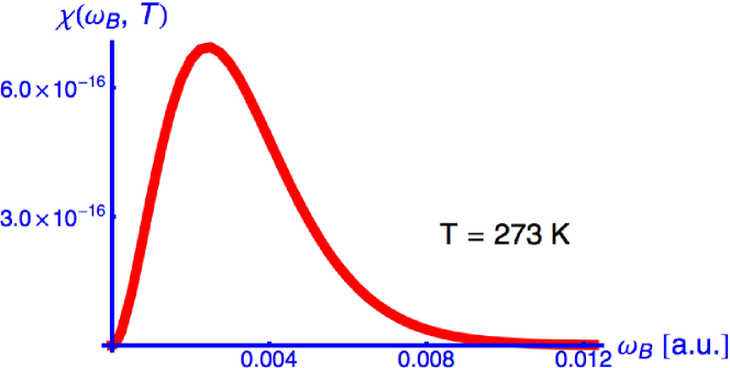
Figure 1: (Color online) $\chi(\omega_{B},T)$ as a function of $\omega_{B}$ at $T=273$ K. The frequency scale is in atomic units (a.u.).

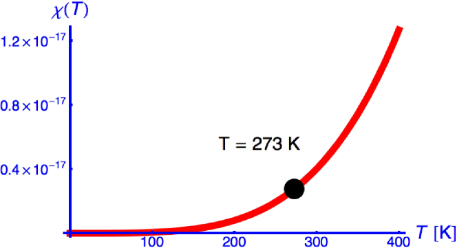
Figure 2: (Color online) A plot of the dimensionless quantity $\chi$ against the temperature $T$ measured in Kelvin (K) is shown, with special emphasis on the point $T=273\,{\rm K}$.

The above calculations illustrate the computational procedure for the static one-color hyperpolarizabilty $\gamma$ and its two-color generalization $\gamma_{2}$. For finite excitation frequency, there is a subtlety which deserves some extra considerations. In the fourth-order matrix elements in Eq. (30), the outer $S$ state couples to odd parity $P$ states by dipole transitions. The inner virtual states can be $S$ or $D$ states, but they can also be even parity $P$ states. Let us suppose that the reference $S$ state has been coupled to a $z$ polarized odd-parity $P$ state. By a dipole transition, emitting or absorbing an $y$ polarized photon, the two-electron system may couple to an even parity $P$ virtual state that is proportional to the $x$ component of the cross product $\vec{r}_{1}\times\vec{r}_{2}$. For $\omega_{B}\to 0$, the contribution of even parity $P$ states vanishes due to symmetry, but it gives a finite effect for nonvanishing $\omega_{B}$. In order to fix the notation, we define

$$\alpha_{PE}=\epsilon_{ijk}\langle\delta\psi_{P}^{i}|r^{j}|\delta\psi_{PE}^{k}\rangle\,,$$ (32)

where the $P$ even ($PE$) states are given by (we invoke the summation convention over $k$ and $l$)

$$|\delta\psi_{PE}^{j}\rangle=\epsilon_{jkl}\,{\cal R}_{PE}(0)r^{k}|\delta\psi_{P}^{l}\rangle$$ (33)

$$\;=\sum_{m=1}^{N_{PE}}v^{PE}_{m}\bigl{[}\epsilon_{jkl}r_{1}^{k}r_{2}^{l}\mathrm{e}^{-a_{i}r_{1}-b_{i}r_{2}-c_{i}r_{12}}-(r_{1}\leftrightarrow r_{2})\bigl{]}\,.$$

We choose $N_{PE}=N_{S}$ and recall the definition of the perturbation $|\delta\psi_{P}^{i}\rangle$ due to the $i$th Cartesian component of the position operator. The definition of $\alpha_{PE}$ thus involves a total of three resolvents of the helium atom. By numerical calculation, using the same incremental values for the basis sets as those indicated in Table 1, we obtain $\alpha_{PE}=-0.062\,951\,884\,22(4)$. This value should not be understood as the static value of a dynamic forth-order polarizability due to even-parity $P$ states (indeed, as outlined above, the contribution of even-parity $P$ states to the two-color hyperpolarizability vanishes). In our definition of $\alpha_{PE}$, we have arranged for the $\epsilon$ tensors to isolate a nonvanishing contribution in the static limit. This approach serves two purposes: (i) to implicitly define the variational parameters used in the calculation of the resolvent ${\cal R}_{PE}$ in both the static as well as the dynamic regime, and (ii) to provide a reference value for the contribution of even-parity $P$ states to a fourth-order matrix element that has a manifestly nonvanishing static limit (but no direct physical interpretation).

For the integration in Eq. (II) over $\omega_{B}$, a 120 point Gauss-Legendre quadrature in the interval $(0,\omega_{B\mathrm{cut}})$ is fully sufficient to obtain

$$\chi=2.742\,57(1)\times 10^{-18}\qquad\mbox{for}\qquad T=273\,{\rm K}\,.$$ (34)

Under the approximation $g(\omega_{B})\approx g(0)$ in Eq. (II), which we can do because $g$ varies slowly on the frequency scale of the Boltzmann distribution at room temperature, the integral over $\omega_{B}$ can by done analytically. It has a character similar to the Stefan-Boltzmann law with a $T^{4}$ temperature dependence. For clarity, we now return to SI MKSA units. With the atomic unit quantities $\overline{\alpha}_{d}=1.383192\dots$ and $\overline{g}(0)=\overline{\gamma}_{2}=59.752019\dots$ defined as in Eq. (20), we obtain

$$\chi\approx \;\frac{4\alpha^{3}}{135}\,\pi^{2}\,\frac{\overline{\gamma}_{2}}{\overline{\alpha}_{d}}\left(\frac{k_{B}T}{E_{h}}\right)^{4}$$

$$\approx \;4.9372\times 10^{-28}\;\left(\frac{T}{\mathrm{K}}\right)^{4}\,.$$ (35)

This approximation gives $\chi=2.7424\times 10^{-18}$ for $T=273\,\mathrm{K}$ with an error of order $10^{-4}$ compared to Eq. (34). At room temperature ($T=300\,\mathrm{K}$), we obtain $\chi=3.999\times 10^{-18}$. Figures 1 and 2 illustrate the Boltzmann weight of the integrand defining $\chi$ and the overall dependence of $\chi$ on the temperature. As indicated in Eq. (16), $\chi$ is the multiplicative factor that gives the temperature-dependent effective static polarizability of helium in the presence of the black-body radiation.

IV Conclusions

We have investigated the effect of black-body radiation on the determination of the helium molar polarizability by fourth-order perturbation theory in the quantized electromagnetic field of the probing microwave and the black-body radiation field. This shift of the molar polarizability is of interest because it may affect a conceivable definition of thermodynamic temperature or a determination of the Boltzmann constant based on the measurement ScGaMaMo2007 . Indeed, it has been suggested in Ref. HoTr1994 that the relative correction to the polarizability amounts to a correction as large as $2.1\times 10^{-10}\,{\rm K}^{-2}\,T^{2}=16\times 10^{-6}$ at $T=273\,\mathrm{K}$, which would have been significant compared to the $9.1\times 10^{-6}$ relative uncertainty of the measurement ScGaMaMo2007 . However, our fourth-order calculations indicate that the effect of black-body radiation on the measurement of the polarizability of helium reported in ScGaMaMo2007 is negligible. In fact, the result of that measurement, $(A_{\epsilon,\mathrm{meas}}-A_{\epsilon,\mathrm{theory}})/A_{\epsilon,\mathrm{theory}}=(1.8\pm 9.1)\times 10^{-6}$, supports this conclusion. The calculation in HoTr1994 considers only the frequency dependence, discussed in Ref. BhDr1998 for example, of the interaction of the black-body radiation with the atoms. In lowest order, this dependence does not affect the interaction of the microwave radiation with the atoms.

Here, we have presented a fully quantized approach to the calculation of the black-body radiation correction to the polarizability of helium, and we have evaluated all expressions numerically [see Eq. (34)] as well as within a semi-analytic approach [see Eq. (III)]. However, even without this formalism, an estimate for the effect of the black-body radiation on the polarizability of helium at room temperature could have been performed based on known literature references, as follows. We start from the ground-state blackbody shift $\delta\nu_{0}=0.11\,\mathrm{Hz}$ given by Farley and Wing FaWi1981 . (This value takes into account the 300 K to 273 K temperature difference as compared to Ref. FaWi1981 .) This amounts to a relative change in the polarizability of order $\delta\nu_{0}/\nu_{\mathrm{He}}\approx 2\times 10^{-17}$, which affects the virtual states in the defining expression for the ground state polarizability (we denote by $\nu_{\mathrm{He}}\approx 5\times 10^{15}\,\mathrm{Hz}$ a typical transition frequency in helium). Unlike the QED corrections, the black-body radiation effect is largest for highly-excited states, so a possibly larger correction would come from the shift of the excited-state energies due to the black-body radiation. These states enter the expression for the polarizability as virtual states, and the relative frequency of the virtual transitions leads to a proportional shift of the polarizability, as implied by the fourth-order effect given in Eq. (19). Farley and Wing find that the correction $\delta\nu_{i}$ for each excited state $i$ approaches a limiting shift of $\delta\nu_{\infty}\to 2.0\,\mathrm{kHz}$ as $i\to\infty$ FaWi1981 . For lower states, this gives an overestimate because the black-body shifts for typical excited states are larger. Nevertheless, if all excited state energies were shifted by this amount, then the polarizability would undergo a relative change of order $\chi(T=273\,{\rm K})=\delta\nu_{\infty}/\nu_{\mathrm{He}}\approx 4\times 10^{-13}$, which needs to be contrasted to our exact result (the latter is in the range of $10^{-18}$ and confirms the overestimation).

In this article, we have carried out a detailed analysis of the effect, and obtained the precise shift of the polarizability in fourth-order perturbation theory, which can be expressed as a relative perturbation of the second order polarizability effect proportional to a dimensionless factor $\chi$. Our analytic formula given in Eq. (III) and our numerical results obtained by numerically integrating the black-body spectrum confirm this estimate under the proviso that the shift of the lowest excited helium states, which is of the order of a few hertz, gives the relevant contribution to the polarizability. In particular, we find a shift of $\chi(T=273\,{\rm K})=2.7424\times 10^{-18}$ for the relative correction to the polarizability of the helium ground state. Furthermore, according to Eq. (III), we find a $T^{4}$ dependence for the overall shift of the polarizability with an analytic dependence of the form $\chi\approx 4.9372\times 10^{-28}(T/\mathrm{K})^{4}$. Although we have carried out numerical calculations only up to a temperature $T=400\,{\rm K}$, an analytic estimate based on the known form of the black-body spectrum shows that the formula Eq. (III) should be valid to better than $1\,\%$ in a temperature range to at least 2000 K.

Finally, we would also like to briefly discuss the size of the effect for other noble gases like neon and argon, which are of experimental interest. The two-color hyperpolarizability scales as $(Z_{\rm eff}\,\alpha)^{-10}$ where $Z_{\rm eff}$ is the effective nuclear charge seen by the electron in the valence shell. The final result for the shift of the polarizability due to the black-body radiation interaction is obtained as an integral over the dynamic two-color hyperpolarizability, and its value may thus additionally depend on the overlap of the resonance frequencies with the maximum of the temperature-dependent black-body spectrum. For temperatures not exceeding $400\,{\rm K}$, however, the static two-color hyperpolarizability of the noble gas in question should provide a good estimate of the total effect, according to Eq. (III). We thus expect that the result for $\chi$ in the temperature range $0<T<400\,{\rm K}$ for neon and argon should not differ from the result given in Eq. (III) by more than two orders of magnitude and thus be negligible on the level of accuracy reached in the experiment ScGaMaMo2007 . More accurate estimates require an explicit calculation of $\gamma_{2}$ for the atomic reference system under investigation.

Appendix A Two-electron integrals

The two-electron integral $\Gamma$ is defined by

$$\Gamma(n_{1},n_{2},n_{3},\alpha,\beta,\gamma)$$

$$\equiv\int\frac{\mathrm{d}^{3}r_{1}}{4\,\pi}\,\int\frac{\mathrm{d}^{3}r_{2}}{4\,\pi}\,\mathrm{e}^{-\alpha\,r_{1}-\beta\,r_{2}-\gamma\,r_{12}}\,r_{1}^{n_{1}-1}\,r_{2}^{n_{2}-1}\,r_{12}^{n_{3}-1}.$$ (36)

This integral takes a very simple form when all $n_{i}=0$,

$$\Gamma(0,0,0,\alpha,\beta,\gamma)=\frac{1}{(\alpha+\beta)\,(\alpha+\gamma)\,(\beta+\gamma)}.$$ (37)

The explicit form for $n_{i}>0$ can be obtained by differentiation with respect to the corresponding parameter. For the actual evaluation of $\Gamma$, we use compact recurrence relations from Refs. SaRoKo1967 ; Ko2000 .

References

- (1) J. W. Schmidt, R. M. Gavioso, E. F. May, and M. R. Moldover, Phys. Rev. Lett. 98, 254504 (2007).
- (2) H. Luther, K. Grohmann, and B. Fellmuth, Metrologia 33, 341 (1996).
- (3) K. Pachucki and J. Sapirstein, Phys. Rev. A 63, 012504 (2000).
- (4) W. Cencek, K. Szalewicz, and B. Jeziorski, Phys. Rev. Lett. 86, 5675 (2001).
- (5) G. Lach, B. Jeziorski, and K. Szalewicz, Phys. Rev. Lett. 92, 233001 (2004).
- (6) M. Haas, U. D. Jentschura, C. H. Keitel, N. Kolachevsky, M. Herrmann, P. Fendel, M. Fischer, Th. Udem, R. Holzwarth, T. W. Hänsch, M. O. Scully, and G. S. Agarwal, Phys. Rev. A 73, 052501 (2006).
- (7) J. J. Sakurai, Modern Quantum Mechanics (Addison-Wesley, Reading, MA, 1994).
- (8) U. D. Jentschura and M. Haas, Phys. Rev. A 78, 042504 (2008).
- (9) S. G. Porsev and A. Derevianko, Phys. Rev. A 74, 020502 (2006).
- (10) M. Haas, U. D. Jentschura, and C. H. Keitel, Am. J. Phys. 74, 77 (2006).
- (11) M. N. Grasso, K. T. Chung, and R. P. Hurst, Phys. Rev. 167, 1 (1968).
- (12) U. D. Jentschura and C. H. Keitel, Ann. Phys. (N.Y.) 310, 1 (2004).
- (13) V. I. Korobov, Phys. Rev. A 61, 064503 (2000).
- (14) V. I. Korobov, Phys. Rev. A 66, 024501 (2002).
- (15) R. A. Sack, C. C. J. Roothaan, and W. Kolos, J. Math. Phys. 8, 1093 (1967).
- (16) D. A. Varshalovich, A. N. Moskalev, and V. K. Khersonskii, Quantum Theory of Angular Momentum (World Scientific, Singapore, 1988).
- (17) D. M. Bishop and J. Pipin, J. Chem. Phys. 91, 3549 (1989).
- (18) U. Hohm and U. Trümper, Chem. Phys. 189, 443 (1994).
- (19) A. K. Bhatia and R. J. Drachman, Phys. Rev. A 58, 4470 (1998).
- (20) J. W. Farley and W. H. Wing, Phys. Rev. A 23, 2397 (1981).