Phase transitions in dipolar spin-$1$ Bose gases

Abstract

We study phase transitions in homogeneous spin-$1$ Bose gases in the presence of long-range magnetic dipole–dipole interactions (DDI). We concentrate on three-dimensional geometries and employ momentum shell renormalization group to study the possible instabilities caused by the dipole–dipole interaction. At the zero-temperature limit where quantum fluctuations prevail, we find the phase diagram to be unaffected by the dipole–dipole interaction. When the thermal fluctuations dominate, polar and ferromagnetic condensates with DDI become unstable and we discuss this crossover in detail. On the other hand, the spin-singlet condensate remains stable in the presence of DDI.

I Introduction

The past few years have revealed that ultracold atomic gases can answer important questions beyond the immediate scope of atomic physics Micheli et al. (2006); Donner et al. (2007); Jördens et al. (2008); Jo et al. (2009). In particular, experimental methods have matured to the level where measurements of critical exponents are possible in some cases Donner et al. (2007). This provides an interesting opportunity to study the physics of phase transitions and critical phenomena utilizing cold atomic gases, as well as to realize exotic phases that are absent in more conventional solid state systems Gorshkov et al. (2010). In this work, we consider Bose gases with a spin degree of freedom Ho (1998); Ohmi and Machida (1998). They provide an intriguing example where magnetic ordering can compete with superfluidity and condensation. This interplay can give rise to a myriad of topological defects Leonhardt and Volovik (2000); Stoof et al. (2001); Al Khawaja and Stoof (2001); Savage and Ruostekoski (2003); Takahashi et al. (2007); Kawaguchi et al. (2008); Pietilä and Möttönen (2009); Huhtamäki et al. (2010); Huhtamäki and Kuopanportti (2010) which play an important role, e.g., in the superfluid transition in low-dimensional systems Mukerjee et al. (2006); Pietilä et al. (2010).

Initially, the magnetic properties of spinor Bose gases were assumed to depend only on the local interactions determined by the scattering lengths in the different total hyperfine spin channels Ho (1998); Ohmi and Machida (1998); Stenger et al. (1998); Schmaljohann et al. (2004); Chang et al. (2004); Sadler et al. (2006), but recent experiments suggest that the long-range magnetic dipole–dipole interaction (DDI) may be an essential ingredient in determining the properties of spinor Bose gases Griesmaier et al. (2005); Lahaye et al. (2007); Koch et al. (2008); Vengalattore et al. (2008, 2010). In this work, we consider the effect of dipole–dipole interaction in spin-$1$ Bose gases using momentum shell renormalization group (RG) Wilson and Kogut (1974); Shankar (1994); Fisher and Hohenberg (1988); Kolomeisky and Straley (1992a, b); Bijlsma and Stoof (1996). We note that also the functional renormalization group Wetterich (1991) has been successfully applied in the context of cold atoms Andersen and Strickland (1999); Andersen (2004); Diehl et al. (2010). The momentum shell RG analysis allows us to determine the effect of DDI on the phase diagram of spin-$1$ Bose gases which has recently attracted some interest Yang (2009); Kolezhuk (2010); Natu and Mueller (2011). Moreover, the recent advances in the creation of Feshbach resonances using either optical means Hamley et al. (2009) or microwaves Papoular et al. (2010), suggest that exploration of the phase diagram could become experimentally realistic in the near future.

Dipole–dipole interaction couples the spin directly to spatial degrees of freedoms, giving local spins tendency to align head to tail and antialign side by side Cherng and Demler (2009); Lahaye et al. (2009). On the other hand, the experiments described in Refs. Vengalattore et al. (2008, 2010) are of mixed dimensionality in the sense that spin dynamics was effectively two-dimensional while otherwise the system was spatially three-dimensional (3D). Furthermore, the original DDI was strongly modified by a rapid Larmor precession induced by an external magnetic field. In the present work, we focus on the properties of pristine DDI and consider a homogeneous three-dimensional system in the absence of external magnetic fields. For three-dimensional systems, DDI is a true long-range interaction Astrakharchik and Lozovik (2008); Lahaye et al. (2009) and we avoid additional complications that may arise due to the absence of true long-range order in low-dimensional systems.

Although dipole–dipole interactions are present in all ferromagnetic materials, they are usually weak and often neglected or treated phenomenologically Ma (1976); Snoke (2008). However, for ferromagnets which order only at very low temperatures, DDI might be crucial for the correct low-energy behavior Belitz and Kirkpatrick (2010). In this work, we analyze this scenario in the context of spin-$1$ Bose gases. We find that DDI introduces additional instabilities to the expected finite-temperature phase diagram Yang (2009). In particular, DDI renders both polar and ferromagnetic condensates unstable and the RG analysis alludes to the existence of a fluctuation-induced first-order transition.

In the zero-temperature limit, we show that DDI renormalizes to zero and the usual mean-field theory Ho (1998); Ohmi and Machida (1998); Lahaye et al. (2009) is a valid description of the system. Dipole–dipole interactions also generate a new single-particle term which has not been taken into account in the previous studies. This new interaction is relevant in the RG sense and it is allowed by the symmetries of the system. However, in the zero-temperature limit it renormalizes to zero along with the DDI.

II The model

We consider a uniform spin-$1$ Bose gas neglecting the effects of an external potential that confines the atoms. In the presence of DDI, the system has a global $U(1)$ symmetry associated with the conserved atom number and a global $SO(3)$ symmetry corresponding to a simultaneous rotation of spin and coordinate spaces Yi and Pu (2006); Kawaguchi et al. (2006). The latter symmetry indicates that only the sum of spin and orbital angular momentum is conserved. The effective action in the Zeeman basis $\{|F=1,m_{\scriptscriptstyle{F}}=+1,0,-1\rangle\}$ can be written as $S=S_{0}+S_{\mathrm{int}}$,

$$S_{0}=\int_{0}^{\hbar\beta}\mathrm{d}\tau\int\mathrm{d}\bm{x}\,\,\psi_{a}^{*}(\bm{x},\tau)\big{(}\hbar\Gamma^{-1}\partial_{\tau}-\frac{\hbar^{2}}{2m}\nabla^{2}-\mu\big{)}\psi_{a}(\bm{x},\tau),$$ (1)

$$S_{\mathrm{int}}=\int_{0}^{\hbar\beta}\mathrm{d}\tau\int\mathrm{d}\bm{x}\,\mathrm{d}\bm{x}^{\prime}\,\bigg{[}\frac{c_{0}}{2}\,|\psi_{a}(\bm{x},\tau)|^{4}\delta(\bm{x}-\bm{x}^{\prime})+\frac{c_{2}}{2}\,|\bm{\mathcal{S}}(\bm{x},\tau)|^{2}\delta(\bm{x}-\bm{x}^{\prime})+$$

$$\hskip 56.9055pt\frac{c_{\mathrm{dd}}}{2}\,\mathcal{S}^{i}(\bm{x},\tau)h^{ij}(\bm{x}-\bm{x}^{\prime})\mathcal{S}^{j}(\bm{x}^{\prime},\tau)\bigg{]},$$ (2)

where $\tau$ is the imaginary time and $\beta=1/k_{\scriptscriptstyle\mathrm{B}}T$. We always assume implicit summation over repeated indices. The local spin is given by $\mathcal{S}^{i}=\psi_{a}^{*}\,\mathcal{F}_{ab}^{i}\,\psi_{b}$, where $\mathcal{F}^{i}$ are spin-$1$ matrices in the Zeeman basis and $\psi_{a}$, $a=-1,0,1$ are bosonic fields. Parameter $\Gamma$ is initially set to unity and it acquires nontrivial renormalization under the RG transformation. In this work we consider two distinct limits: the $T=0$ case where $\Gamma$ renormalizes only due to the anomalous dimension of the fields $\psi_{a}$ and the high temperature limit where $\Gamma$ renormalizes to zero and we obtain a classical theory.

The bare values of the coupling constants $c_{0}$ and $c_{2}$ are related to scattering lengths $a_{0}$ and $a_{2}$ in the total hyperfine spin channels $F=0$ and $F=2$ by $c_{0}=4\pi\hbar^{2}(a_{0}+2a_{2})/3m$ and $c_{2}=4\pi\hbar^{2}(a_{2}-a_{0})/3m$. The coupling constant corresponding to DDI is given by $c_{\mathrm{dd}}=\mu_{0}\mu_{\scriptscriptstyle\mathrm{B}}^{2}g_{\scriptscriptstyle\mathrm{F}}^{2}/4\pi$, where $\mu_{0}$ is the vacuum permeability, $\mu_{\scriptscriptstyle\mathrm{B}}$ Bohr magneton, and $g_{\scriptscriptstyle\mathrm{F}}$ Landé $g$-factor. The kernel for dipole–dipole interactions in the momentum space takes the form Cherng and Demler (2009)

$$h^{ij}(\bm{q})=-\frac{4\pi}{3}(\delta^{ij}-3\hat{q}^{i}\hat{q}^{j}).$$ (3)

In real space, $h^{ij}(\bm{r})$ decays as $1/|\bm{r}|^{3}$. To date, the only experimentally studied dipolar spin-$1$ Bose gas has been ⁸⁷Rb for which the different coupling constants satisfy $c_{2}/c_{0}=-0.005$ and $c_{\mathrm{dd}}/|c_{2}|=0.1$ Vengalattore et al. (2008). Another candidate for dipolar spin-$1$ Bose gas is ²³Na for which the scattering lengths of Ref. Burke et al. (1998) give $c_{2}/c_{0}=0.03$ and $c_{\mathrm{dd}}/c_{2}=0.006$. The small value of $c_{\mathrm{dd}}/c_{2}$ explains why the effects arising from DDI have been expected to be vanishingly small for ²³Na. The different interaction vertices appearing in the RG calculations in Sections III–VI are illustrated in Fig. 1.

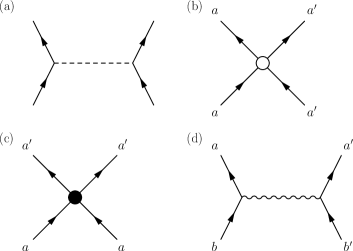
Figure 1: (a) Generic interaction vertex, (b) local density–density interaction, (c) local spin-spin interaction, (d) and dipole–dipole interaction. The generic interaction vertex (a) can denote any of the vertices (b)–(d). Conservation of the 4-momentum $\vec{k}=(\omega_{n},\bm{k})$ at each vertex is implied.

To streamline the RG calculations, we switch to the Cartesian basis. In this basis, the field operator $\Psi=(\psi_{x},\psi_{y},\psi_{z})$ transforms as a vector under spin rotations. Moreover, the spin-1 matrices $(\mathcal{F}_{x},\mathcal{F}_{y},\mathcal{F}_{z})$ take a particularly simple form $(\mathcal{F}_{\alpha})_{\beta\gamma}=-i\varepsilon_{\alpha\beta\gamma}$, where $\varepsilon_{\alpha\beta\gamma}$ is the Levi-Civita tensor. The effective action can be written as

$$S_{0} =\int\mathrm{d}^{4}k\,\,\psi_{\alpha}^{*}(\vec{k})\big{(}-i\hbar\Gamma^{-1}\omega_{n}+\varepsilon_{\bm{k}}-\mu\big{)}\psi_{\alpha}(\vec{k}),$$ (4)

$$S_{\mathrm{int}} =\int\,\frac{\mathrm{d}^{4}k\,\mathrm{d}^{4}p\,\mathrm{d}^{4}q}{(2\pi)^{3}\hbar\beta}\,\bigg{[}\frac{g_{d}}{2}\,\psi_{\alpha}^{*}(\vec{p}+\vec{q})\psi_{\alpha^{\prime}}^{*}(\vec{k}-\vec{q})\psi_{\alpha^{\prime}}(\vec{k})\psi_{\alpha}(\vec{p})$$

$$\hskip 8.53581pt+\,\frac{g_{s}}{2}\,\psi_{\alpha}^{*}(\vec{p}+\vec{q})\psi_{\alpha}^{*}(\vec{k}-\vec{q})\psi_{\alpha^{\prime}}(\vec{k})\psi_{\alpha^{\prime}}(\vec{p})$$

$$+ \,\frac{c_{\mathrm{dd}}}{2}\,\psi_{\alpha}^{*}(\vec{p}+\vec{q})\psi_{\alpha^{\prime}}^{*}(\vec{k}-\vec{q})\,h^{ij}(\bm{q})\mathcal{F}_{\alpha\beta}^{i}\mathcal{F}_{\alpha^{\prime}\beta^{\prime}}^{j}\,\psi_{\beta^{\prime}}(\vec{k})\psi_{\beta}(\vec{p})\bigg{]},$$ (5)

where indices $\{x,y,z\}$ are referred to by the Greek indices $\alpha,\beta,...$ and the Latin indices $a,b,...$ correspond to the original Zeeman basis. We use a shorthand notation $\vec{k}=(\omega_{n},\bm{k})$ and $\int\mathrm{d}^{4}k=\sum_{\omega_{n}}\int\mathrm{d}\bm{k}$. Bosonic Matsubara frequencies are given by $\omega_{n}=2\pi n/\hbar\beta$ and $\varepsilon_{\bm{k}}=\hbar^{2}\bm{k}^{2}/2m$. The coupling constants $g_{d}$ and $g_{s}$ are related to the coupling constants in the Zeeman basis by $g_{d}=c_{0}+c_{2}$ and $g_{s}=-c_{2}$.

III Renormalization group calculation

We set up the RG calculation in a fixed dimension $D$ following Refs. Fisher and Hohenberg (1988); Kolomeisky and Straley (1992a, b); Bijlsma and Stoof (1996). To make a connection to Refs. Yang (2009); Kolezhuk (2010), we first neglect the dipole–dipole interactions and study a general $D$-dimensional situation. We show that our RG equations at the zero-temperature limit coincide with Ref. Kolezhuk (2010) and essentially reproduce the phase diagram proposed in Ref. Yang (2009). We also point out that in a contrast to Ref. Kolezhuk (2010), in which the stability of low-dimensional multi-component Bose gases was considered at the zero-temperature limit, our main focus is a three dimensional spinor Bose gas at finite temperatures. We note that isotropic long-range interactions in spinless Bose gases have been analyzed in the zero-temperature limit in Ref. Kolomeisky and Straley (1992b) and long-range interactions of the form $V(\bm{r})\propto 1/|\bm{r}|^{s}$ were found irrelevant for $s>2$. Our findings in the presence of DDI are similar to those of Ref. Kolomeisky and Straley (1992b), namely, DDI becomes irrelevant at zero temperature.

To study the effects of DDI, we employ the momentum shell RG Wilson and Kogut (1974); Shankar (1994); Bijlsma and Stoof (1996) in which we split the fields appearing in Eqs. (4) and (II) such that $\psi_{\alpha}=\psi_{\alpha,<}+\psi_{\alpha,>}$, where the $\psi_{\alpha,<}$ contains momentum components with $|\bm{k}|<\Lambda/s$ and $\psi_{\alpha,>}$ corresponds to momenta $\Lambda/s\leq|\bm{k}|<\Lambda$. The ultraviolet (UV) cutoff is denoted by $\Lambda$, and in general, nonuniversal quantities such as condensate fraction or critical temperature depend explicitly on $\Lambda$. Several tricks such as halting the RG flow when an appropriate scale is reached or relating $\Lambda$ to the $s$-wave scattering length can be used to obtain information on quantities depending on $\Lambda$ Kolezhuk (2010); Fisher and Hohenberg (1988); Kolomeisky and Straley (1992a, b); Bijlsma and Stoof (1996).

The RG calculation proceeds by integrating out the fast modes residing at the momentum shell $\Lambda/s\leq|\bm{k}|<\Lambda$, which results in a renormalized action for the slow modes $\psi_{\alpha,<}$. At the second step of RG transformation, the UV cutoff is brought back to the original value $\Lambda$ by rescaling the fields and momenta, giving rise to RG equations for the chemical potential and coupling constants. Only the one-particle irreducible connected diagrams contribute to the RG equations. In this work, we compute the RG equations to the one-loop order. The relevant diagrams appearing in the renormalization of chemical potential and coupling constants are shown Figs. 2 and 3.

Figure 2: One-loop diagrams contributing to renormalization of the chemical potential. The interaction line can be any of those denoted in Fig. 1(b)–(d). The external legs corresponding to fields $\psi_{\alpha,<}$ and $\psi_{\alpha,<}^{*}$ are denoted by gray lines for clarity. The dipole–dipole interaction can give rise to external interaction lines which are also denoted by gray dashed lines [the tadpole diagram in (a)].

The diagrams in Figs. 2 and 3 correspond to an expansion with respect to coupling constants $g_{d}$, $g_{s}$, and $c_{\mathrm{dd}}$ in the first non-trivial order. The internal lines are evaluated using non-interacting one-particle Green’s function

$$\mathcal{G}_{0,\alpha\beta}(\bm{k},\omega_{n})=-\frac{\hbar}{-i\hbar\Gamma^{-1}\omega_{n}+\varepsilon_{\bm{k}}-\mu}\delta_{\alpha\beta}.$$ (6)

After integrating out the fast modes and neglecting the irrelevant terms generated by the momentum shell integration, the slow fields, momentum, and imaginary time are rescaled as Fisher and Hohenberg (1988)

$$\bm{k}\rightarrow\bm{k}\,e^{-\ell},$$ (7a)

$$\tau\rightarrow\tau\,e^{z\ell},$$ (7b)

$$\psi_{\alpha}\rightarrow\psi_{\alpha}\,e^{\zeta\ell},$$ (7c)

where we have taken $s=e^{\ell}$. For simplicity, we first neglect the anomalous dimension of the fields, which allows us to keep the kinetic energy term in Eq. (4) fixed during the RG transformation. In Section VI, we take into account also the renormalization of the kinetic energy term and find that $\varepsilon_{\bm{k}}$ is only weakly renormalized. For vanishing anomalous dimension we obtain an identity Fisher and Hohenberg (1988)

$$2\zeta+z=2-D,$$ (8)

and the relevance of all other terms is compared to the kinetic energy. The requirement that the rescaled action is equivalent to the original one yields the scaling relations

$$\Gamma\rightarrow\Gamma\,e^{(d+2\zeta)\ell},$$ (9a)

$$\mu\rightarrow\mu\,e^{-2\ell},$$ (9b)

$$g\rightarrow g\,e^{-2(\zeta+1)\ell},$$ (9c)

$$T\rightarrow T\,e^{-z\ell}$$ (9d)

where $g=g_{d},g_{s},c_{\mathrm{dd}}$, and we have used Eq. (8). In the presence of DDI, we take $D=3$.

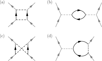
Figure 3: One-loop diagrams contributing to renormalization of coupling constants $g_{d}$, $g_{s}$, and $c_{\mathrm{dd}}$. The two interaction lines can be any combination of the interactions in Fig. 1(b)–(d). The external legs and interaction lines are again denoted by gray color.

In general, RG calculations provide information on universal quantities such as different phases and transitions between them. On the other hand, renormalization group analysis can be used to determine the relevance of a particular interaction for a given phase and to study the stability of different phases when additional interactions are included. We take the latter point of view in Sections IV–VI where we analyze the effects of DDI on the phase diagram of spin-$1$ Bose gases.

IV RG flow in the absence of dipole–dipole interactions

Let us first consider a general dimension $D$ and neglect DDI. The different diagrams contributing to the RG equations are shown in Fig. 4. Since all interactions are local, the different diagrams in Fig. 4 reduce to evaluation of the bubbles shown in Fig. 5. Integration on the momentum shell is restricted to the interval $\Lambda/s\leq|\bm{k}|<\Lambda$ and the Matsubara sums can be calculated using the standard methods Bruus and Flensberg (2004). At the limit of an infinitesimal shell of thickness $\Lambda d\ell$, we obtain

$$\mathrm{d}\mu=-2(g_{s}+2g_{d})K_{D}\Gamma\,n_{\scriptscriptstyle\mathrm{BE}}[\beta\Gamma(\varepsilon_{\Lambda}-\mu)]\Lambda^{D}\mathrm{d}\ell,$$ (10)

$$\mathrm{d}g_{s}=-[(3g_{s}^{2}+2g_{d}g_{s})\chi_{1}+4g_{d}g_{s}\chi_{2}]K_{D}\Lambda^{D}\mathrm{d}\ell,$$ (11)

$$\mathrm{d}g_{d}=-[g_{d}^{2}\chi_{1}+4(g_{d}^{2}+g_{d}g_{s}+g_{s}^{2})\chi_{2}]K_{D}\Lambda^{D}\mathrm{d}\ell,$$ (12)

where $K_{D}=[2^{D-1}\pi^{D/2}\Gamma(D/2)]^{-1}$ and $\Gamma(x)$ is the Gamma function (not to be confused with the energy parameter $\Gamma$). Furthermore, functions $\chi_{1}(\beta,\Gamma)$ and $\chi_{2}(\beta,\Gamma)$ are given by

$$\chi_{1}(\beta,\Gamma)=\Gamma\,\frac{1+2n_{\scriptscriptstyle\mathrm{BE}}[\beta\Gamma(\varepsilon_{\Lambda}-\mu)]}{2(\varepsilon_{\Lambda}-\mu)},$$ (13)

$$\chi_{2}(\beta,\Gamma)=\beta\Gamma^{2}\,n_{\scriptscriptstyle\mathrm{BE}}[\beta\Gamma(\varepsilon_{\Lambda}-\mu)]\{1+n_{\scriptscriptstyle\mathrm{BE}}[\beta\Gamma(\varepsilon_{\Lambda}-\mu)]\}.$$ (14)

We have denoted the Bose distribution function by $n_{\scriptscriptstyle\mathrm{BE}}(x)=1/(e^{x}-1)$ and $\varepsilon_{\Lambda}=\hbar^{2}\Lambda^{2}/2m$. The contributions proportional to $\chi_{1}$ correspond to diagrams containing the bubble in Fig. 5(a) and contributions containing $\chi_{2}$ arise from diagrams with the bubble in Fig. 5(b).

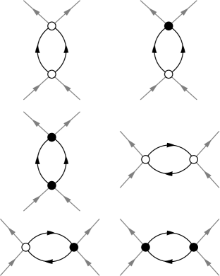
Figure 4: One-loop contributions to RG equations in the absence of dipole–dipole interactions.

Taking into account the scalings dictated by Eqs. (7) and (9), using the scaling relation in Eq. (8), and transforming back to the Zeeman basis we obtain the following flow equations

$$\frac{\mathrm{d}\beta}{\mathrm{d}\ell}=-z\beta,$$ (15)

$$\frac{\mathrm{d}\Gamma}{\mathrm{d}\ell}=-(2\zeta+D)\Gamma,$$ (16)

$$\frac{\mathrm{d}\mu}{\mathrm{d}\ell}=2\mu-2(c_{2}+2c_{0})K_{D}\Lambda^{D}\Gamma\,n_{\scriptscriptstyle\mathrm{BE}}[\beta\Gamma(\varepsilon_{\Lambda}-\mu)],$$ (17)

$$\frac{\mathrm{d}c_{0}}{\mathrm{d}\ell}=2(\zeta+1)c_{0}-[(c_{0}^{2}+2c_{2}^{2})\chi_{1}+4c_{0}^{2}\chi_{2}]K_{D}\Lambda^{D},$$ (18)

$$\frac{\mathrm{d}c_{2}}{\mathrm{d}\ell}=2(\zeta+1)c_{2}-[(2c_{0}c_{2}-c_{2}^{2})\chi_{1}$$

$$\hskip 105.2751pt+4(c_{0}c_{2}+c_{2}^{2})\chi_{2}]K_{D}\Lambda^{D}.$$ (19)

Although these equation are valid for any temperature, we consider two limits: the quantum regime which takes place at the zero-temperature limit and is dominated by the quantum fluctuations, and the thermal regime where thermal fluctuations prevail over the quantum fluctuations Fisher and Hohenberg (1988).

Figure 5: Basic bubbles for diagrams in the absence of dipole–dipole interactions. The bubbles depend in principle on external momenta. Expanding about the zero momentum one observes that terms corresponding to finite external momentum are at most marginal in the RG sense. Since we have neglected marginal interactions from the outset, we take the external momenta to be zero.

IV.1 Quantum regime

Let us first consider the quantum regime at which we require $\mathrm{d}\Gamma/\mathrm{d}\ell=0$. Furthermore, we set $\Gamma=1$. From Eqs. (8) and (16) we obtain $\zeta=-D/2$ and $z=2$. This gives the usual instability of the $T^{*}=0$ fixed point, since any nonzero temperature tends to increase in the RG flow. In the limit $k_{\scriptscriptstyle\mathrm{B}}T\ll\varepsilon_{\Lambda}-\mu$, we have

$$\chi_{1}(\beta,\Gamma)\rightarrow\frac{1}{2(\varepsilon_{\Lambda}-\mu)},$$

$$\chi_{2}(\beta,\Gamma)\rightarrow 0,$$

where the latter equation gives the well-known result stating that in the zero-temperature limit, only the ladder diagrams contribute to the renormalization Sachdev (1999). The RG equation for the chemical potential becomes $\mathrm{d}\mu/\mathrm{d}\ell=2\mu$, and the only fixed point is $\mu^{*}=0$. Furthermore, the remaining RG equations reduce to

$$\frac{dc_{0}}{d\ell}=(2-D)c_{0}-(c_{0}^{2}+2c_{2}^{2})\frac{K_{D}\Lambda^{D}}{2\varepsilon_{\Lambda}},$$ (20)

$$\frac{dc_{2}}{d\ell}=(2-D)c_{2}+(c_{2}^{2}-2c_{0}c_{2})\frac{K_{D}\Lambda^{D}}{2\varepsilon_{\Lambda}}.$$ (21)

The above equations are precisely those of Ref. Kolezhuk (2010), and for the future reference, we consider here the $D=3$ case. Cases $D=1$ and $D=2$ have been analysed in Ref. Kolezhuk (2010).

	I	II	III	IV
$\hat{c}_{0}^{*}$	$0$	$\frac{1}{3}(2-D)$	$\frac{2}{3}(2-D)$	$2-D$
$\hat{c}_{2}^{*}$	$0$	$\frac{1}{3}(D-2)$	$\frac{1}{3}(2-D)$	$0$

Table 1: Different fixed points corresponding to the RG equations (20) and (21). The dimensionless values are defined as $\hat{c}_{i}^{*}=2\varepsilon_{\Lambda}c_{i}^{*}/K_{D}\Lambda^{D}$, $i=0,2$. In three dimensions, the Gaussian fixed point I is stable and the $SU(3)$ symmetric fixed point IV is unstable. Fixed points II and III have both relevant and irrelevant scaling fields.

The fixed points corresponding to the RG flow defined by Eqs. (20) and (21) can be determined exactly. The four different fixed points are given in Table 1, and the RG flow for $D=3$ is shown in Fig. 6. The fixed points $\hat{c}_{0}^{*}$ and $\hat{c}_{2}^{*}$ correspond to the dimensionless values $\hat{c}_{i}^{*}=2\varepsilon_{\Lambda}c_{i}^{*}/K_{D}\Lambda^{D}$, for $i=0,2$. In the special case $D=2$, the dimensionless quantities are independent of $\Lambda$ Kolezhuk (2010). The RG flows in Fig. 6 show that similarly to the $D=1$ and $D=2$ cases, there are two runaway flows indicating the formation of bound spin singlet pairs (positive $c_{2}$) and ferromagnetic instability (negative $c_{2}$) where the condensate becomes locally fully spin-polarized in the sense that fluctuations in the magnitude of the local spin become suppressed.

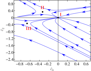
Figure 6: (Color online) Renormalization group flow for a three dimensional spin-$1$ Bose gas at zero temperature in the absence of dipole–dipole interactions. The dimensionless coupling constants are defined as $\hat{c}_{i}=2\varepsilon_{\Lambda}c_{i}/K_{3}\Lambda^{3}$, $i=0,2$. The Gaussian fixed point (I) is stable, and RG flows starting from $\hat{c}_{0}\geq 0$ and small $|\hat{c}_{2}|$ end up to the Gaussian fixed point. Fixed points II and III are in the physically inaccessible region but they still have an effect on the RG flow since they give rise to two runaway flows for large $|\hat{c}_{2}|$.

The runaway flow associated with the formation of pair condensate renders the coupling $g_{0}=c_{0}-2c_{2}$ corresponding to the spin singlet channel negative, while the coupling $g_{2}=c_{0}+c_{2}$ in the $F=2$ channel remains positive. Hence this instability corresponds to formation of spin singlet pairs. The second runaway flow where $c_{2}$ becomes ever more negative renders both $g_{0}$ and $g_{2}$ negative. We refer to these two instabilities as antiferromagnetic (AFM) and ferromagnetic (FM) runaway flow, respectively.

At mean-field level, stability of a finite cloud against collapse requires the bare coupling constants to satisfy $c_{0}\geq 0$ and $-c_{2}\leq c_{0}$ Yang (2009). On the other hand, the flow diagram in Fig. 6 indicates that many-body corrections yield a larger window of coupling constants $\hat{c}_{0}$ and $\hat{c}_{2}$ which renormalize to the Gaussian fixed point. Although both FM and AFM runaway flows suggest that the system becomes unstable, stability can be restored by including the higher order terms generated by the RG transformation. Such terms in general are marginal or irrelevant in the RG sense, but can nevertheless become important in the regime where RG flow does not converge to any fixed point Rudnick (1978); Amit and Martín-Mayor (2005).

Between the regions corresponding to AFM and FM runaway flows, the gas forms the usual spinor condensate. Since interactions tend to renormalize to the Gaussian fixed point, the Bogoliubov mean-field theory of spinor condensates is a valid description of the system in this regime (cf. Ref. Fisher and Hohenberg (1988)). However, the RG approach used here does not provide information about nonuniversal properties such as the possible fragmentation of the condensate for antiferromagnetic interactions Ho and Yip (2000).

IV.2 Thermal regime

In the thermal regime, we require that $\beta$ in Eq. (15) does not flow, i.e., the temperature is kept constant in the RG flow. This implies $z=0$, and Eq. (8) gives $\zeta=(2-D)/2$. From Eq. (16) we observe that any finite initial $\Gamma_{0}$ flows to zero. Quantum fluctuations are thus negligible in this limit and we take $\Gamma\rightarrow 0$ in Eqs. (17)–(IV). We obtain

$$\Gamma\,n_{\scriptscriptstyle\mathrm{BE}}[\beta\Gamma(\varepsilon_{\Lambda}-\mu)]\rightarrow\frac{1}{\beta(\varepsilon_{\Lambda}-\mu)},$$ (22)

$$\chi_{1}(\beta,\Gamma)\rightarrow\frac{1}{\beta(\varepsilon_{\Lambda}-\mu)^{2}},$$ (23)

$$\chi_{2}(\beta,\Gamma)\rightarrow\frac{1}{\beta(\varepsilon_{\Lambda}-\mu)^{2}},$$ (24)

and at the critical plane corresponding to $\mu=0$ rg_ ; Aha we have

$$\frac{dc_{0}}{d\ell}=(4-D)c_{0}-(5c_{0}^{2}+2c_{2}^{2})\frac{K_{D}\Lambda^{D}}{\beta\varepsilon_{\Lambda}^{2}},$$ (25)

$$\frac{dc_{2}}{d\ell}=(4-D)c_{2}-(3c_{2}^{2}+6c_{0}c_{2})\frac{K_{D}\Lambda^{D}}{\beta\varepsilon_{\Lambda}^{2}}.$$ (26)

At finite temperatures we define dimensionless coupling constants by $\hat{c}_{i}=\beta\varepsilon_{\Lambda}^{2}c_{i}/K_{D}\Lambda^{D}$, $i=0,2$. Note that the definition is slightly different from the zero-temperature case. Fixed points corresponding to the dimensionless coupling constants are shown in Table 2, where have defined $\epsilon=4-D$.

	I	II	III	IV
$\hat{c}_{0}^{*}$	$0$	$0.088\epsilon$	$0.194\epsilon$	$0.2\epsilon$
$\hat{c}_{2}^{*}$	$0$	$0.157\epsilon$	$-0.054\epsilon$	$0$

Table 2: Fixed points corresponding to the RG equations (25) and (26). The dimensionless values are defined as $\hat{c}_{i}^{*}=\beta\varepsilon_{\Lambda}^{2}c_{i}^{*}/K_{D}\Lambda^{D}$, $i=0,2$. The Gaussian fixed point I is unstable and the $SU(3)$-symmetric fixed point IV is stable for $\epsilon>0$ ($D<4$). Fixed points II and III have both relevant and irrelevant scaling fields.

To analyze the RG equations in the absence of DDI, we concentrate on the case $D=3$ for which the RG flows are depicted in Fig. 7. The instabilities indicated by the runaway flows have the same structure and physical interpretation as in the zero-temperature case. An interesting difference to the zero-temperature limit is that the ferromagnetic instability corresponding to the runaway flows for large negative $c_{2}$ takes place before the mean-field criterion $c_{0}\geq 0$ and $-c_{2}\leq c_{0}$ is violated. Hence, the thermal fluctuations tend to decrease the stability of spinor condensates on the ferromagnetic side ($c_{2}<0$).

We note that only the ratio $\hat{c}_{2}/\hat{c}_{0}$ is universal (i.e., independent of the cutoff $\Lambda$), and therefore quantitative comparison of the singlet condensate formation in the quantum and thermal regimes depends on $\Lambda$, see Figs. 6 and 7. The values $c_{2}/c_{0}$ discussed in Sec. II place the bare coupling constants $\hat{c}_{0}(0)$ and $\hat{c}_{2}(0)$ for ²³Na and ⁸⁷Rb into the regime where $\hat{c}_{0}(\ell)$ and $\hat{c}_{2}(\ell)$ either renormalize to zero (quantum limit) or to the $SU(3)$ symmetric fixed point where $\hat{c}_{2}^{*}=0$ (thermal limit). Since ferromagnetic and antiferromagnetic (polar) condensates correspond to different symmetries, they should be separated by a phase transition. At mean-field level, we expect the transition to be first order (see also Ref. Yang (2009)). The RG calculation supports this conclusion in the sense that we do not find a critical point separating the two phases, see Fig. 7.

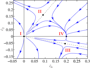
Figure 7: (Color online) Renormalization group flow for a three dimensional spin-$1$ Bose gas at fixed temperature. The RG flows correspond to the case where dipole–dipole interactions are either absent or take the fixed-point value $c_{\mathrm{dd}}^{*}=0$. The dimensionless coupling constants are defined as $\hat{c}_{i}=\beta\varepsilon_{\Lambda}^{2}c_{i}/K_{3}\Lambda^{3}$, $i=0,2$. The ferromagnetic condensate corresponds to the region with $\hat{c}_{2}<0$ above the lower dashed line. The region of antiferromagnetic condensate is delimited by $\hat{c}_{2}>0$ and the upper dashed line.

At first it may seem surprising that the fixed point IV (or the Gaussian fixed point I at $T=0$) governs the properties of both antiferromagnetic and ferromagnetic condensates. However, according to the exact theorem of Ref. Eisenberg and Lieb (2002), the correct low-energy theory of spin-$1$ bosons should indeed correspond to $c_{2}=0$. The authors of Ref. Eisenberg and Lieb (2002) propose that a nonzero $c_{2}$ in the low-energy theory could arise either from dipole–dipole interactions or from the electron transfer between the atoms. In Secs. V and VI we show that DDI is indeed sufficient to give rise to nonzero $c_{2}$ in the low-energy description of spinor Bose gases. Since several important properties of the spinor Bose gases hinge upon the presupposition that the spin-dependent coupling is nonzero Leonhardt and Volovik (2000); Stoof et al. (2001); Al Khawaja and Stoof (2001); Savage and Ruostekoski (2003); Kawaguchi et al. (2008); Mukerjee et al. (2006); Pietilä et al. (2010); Takahashi et al. (2007); Huhtamäki et al. (2010); Pietilä and Möttönen (2009), the analysis in Secs. V and VI provides justification for this key assumption. The two runaway flows do not contradict the aforementioned theorem since they correspond to the formation of a spinless condensate consisting of either single atoms polarized to the same hyperfine spin state or spin singlet pairs.

V RG analysis of dipolar Bose gas

We calculate contributions arising from DDI using the generic diagrams depicted in Figs. 2 and 3. The contribution from the tadpole diagram in Fig. 2(a) vanishes identically for DDI, and the rainbow diagram in Fig. 2(b) does not contribute to the renormalization of chemical potential. However, the rainbow diagram does in principle contribute to the anomalous dimension $\eta$ which indicates the importance of renormalization of the kinetic energy term in Eq. (4). At this point, we neglect the renormalization $\varepsilon_{\bm{k}}\rightarrow Z_{\eta}\varepsilon_{\bm{k}}$ altogether and set $Z_{\eta}=1$. We will justify this assumption after we have derived the full RG equations in Sec. IV.

The rainbow diagram also generates a relevant term which in the Cartesian basis takes the simple form

$$S_{0}^{\prime}=-h_{0}\int\mathrm{d}^{4}k\,\,\psi_{\alpha}^{*}(\vec{k})\,k_{\alpha}k_{\beta}\,\psi_{\beta}(\vec{k}),\,\,\,\,\alpha,\beta\in\{x,y,z\}.$$ (27)

We have introduced here a new coupling constant $h_{0}$ that is determined by the RG equations. At the lowest order, $h_{0}$ is proportional to $c_{\mathrm{dd}}$. We note that the combined contribution of the kinetic energy renormalization and $S_{0}^{\prime}$ can be written as a squared spin-orbit interaction

$$S_{\mathrm{so}}=\int\mathrm{d}^{4}k\,\,\psi_{\alpha}^{*}(\vec{k})\,(\bm{k}\cdot\bm{\mathcal{F}})^{2}_{\alpha\beta}\,\psi_{\beta}(\vec{k}).$$ (28)

The new single-particle term $S_{0}^{\prime}$ is allowed since it has the same symmetries as the original action given by Eqs. (4) and (II). Whether this term should be included to the original action from the beginning depends on the behaviour of $c_{\mathrm{dd}}(\ell)$ in the RG flow and, in particular, on the values of $c_{\mathrm{dd}}(\ell)$ at the fixed points.

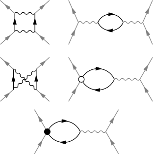
Figure 8: Additional one-loop diagrams giving a nonzero contribution to the RG equations in the presence of dipole–dipole interactions.

Most of the diagrams in Fig. 3 do not contribute to the renormalization of the coupling constants. All the relevant terms are shown in Fig. 8, and they can be evaluated using essentially the same methods as in Sec. IV. They yield

$$\mathrm{d}g_{s}=(\lambda_{1}c_{\mathrm{dd}}^{2}\chi_{1}+\lambda_{2}c_{\mathrm{dd}}^{2}\beta\chi_{2})K_{3}\Lambda^{3}\mathrm{d}\ell$$ (29)

$$\mathrm{d}g_{d}=-(\lambda_{3}c_{\mathrm{dd}}^{2}\chi_{1}+\lambda_{4}c_{\mathrm{dd}}^{2}\beta\chi_{2})K_{3}\Lambda^{3}\mathrm{d}\ell$$ (30)

$$\mathrm{d}c_{\mathrm{dd}}=-(\lambda_{5}c_{\mathrm{dd}}^{2}+2c_{\mathrm{dd}}g_{d}-4c_{\mathrm{dd}}g_{s})K_{3}\chi_{2}\Lambda^{3}\mathrm{d}\ell,$$ (31)

where $\lambda_{1}=32\pi^{2}/45$, $\lambda_{2}=272\pi^{2}/45$, $\lambda_{3}=256\pi^{2}/45$, $\lambda_{4}=496\pi^{2}/45$, and $\lambda_{5}=8\pi/3$. The complete set of RG equations for a dipolar Bose gas consists of contributions from Eqs. (29)–(31) and the RG equations (15)–(IV). We consider again the same limits as in Sec. IV, namely, the quantum limit $T\rightarrow 0$ and the thermal limit $\Gamma\rightarrow 0$.

V.1 Quantum regime

Using the results of Sec. IV.1, we obtain the RG equations for nonzero dipole–dipole interaction at the fixed point $\mu^{*}=0$

$$\frac{\mathrm{d}c_{0}}{\mathrm{d}\ell}=-c_{0}-(c_{0}^{2}+2c_{2}^{2}+\gamma_{1}c_{\mathrm{dd}}^{2})\frac{K_{3}\Lambda^{3}}{2\varepsilon_{\Lambda}},$$ (32)

$$\frac{\mathrm{d}c_{2}}{\mathrm{d}\ell}=-c_{2}+(c_{2}^{2}-2c_{0}c_{2}-\gamma_{2}c_{\mathrm{dd}}^{2})\frac{K_{3}\Lambda^{3}}{2\varepsilon_{\Lambda}},$$ (33)

$$\frac{\mathrm{d}c_{\mathrm{dd}}}{\mathrm{d}\ell}=-c_{\mathrm{dd}},$$ (34)

where $\gamma_{1}=224\pi^{2}/45$ and $\gamma_{2}=32\pi^{2}/45$. We observe immediately that the dipole–dipole coupling constant $c_{\mathrm{dd}}$ renormalizes exponentially to zero in the zero-temperature limit, and the new single-particle term Eq. (27) remains unimportant. The fixed points of the RG flow are shown in Table 1 with an addition that $c_{\mathrm{dd}}^{*}=0$ at each fixed point. Furthermore, since $c_{\mathrm{dd}}$ appears quadratically in Eqs. (32) and (33), the stability of the fixed points is not affected by DDI and $c_{\mathrm{dd}}$ gives rise to an irrelevant scaling field at these fixed points. Otherwise the properties of RG flows are the same as in Sec. IV.1.

V.2 Thermal regime

In the thermal regime, we require again that the temperature does not flow under RG, which renders the parameter $\Gamma$ to renormalize exponentially to zero. Using Eqs. (22)–(24), we obtain, for $\mu^{*}=0$

$$\frac{\mathrm{d}c_{0}}{\mathrm{d}\ell}=c_{0}-(5c_{0}^{2}+2c_{2}^{2}+\alpha_{0}c_{\mathrm{dd}}^{2})\frac{K_{3}\Lambda^{3}}{\beta\varepsilon_{\Lambda}^{2}},$$ (35)

$$\frac{\mathrm{d}c_{2}}{\mathrm{d}\ell}=c_{2}-(3c_{2}^{2}+6c_{0}c_{2}+\alpha_{2}c_{\mathrm{dd}}^{2})\frac{K_{3}\Lambda^{3}}{\beta\varepsilon_{\Lambda}^{2}},$$ (36)

$$\frac{\mathrm{d}c_{\mathrm{dd}}}{\mathrm{d}\ell}=c_{\mathrm{dd}}-(\alpha_{\mathrm{dd}}c_{\mathrm{dd}}^{2}+2c_{0}c_{\mathrm{dd}}+6c_{2}c_{\mathrm{dd}})\frac{K_{3}\Lambda^{3}}{\beta\varepsilon_{\Lambda}^{2}},$$ (37)

where $\alpha_{0}=448\pi^{2}/45$, $\alpha_{2}=304\pi^{2}/45$, and $\alpha_{\mathrm{dd}}=8\pi/3$. The RG flow gives rise to the four fixed points discussed in Sec. IV.2 corresponding to $c_{\mathrm{dd}}^{*}=0$. There are also two additional fixed points given by

$$\hat{c}_{0}^{*}=0.087,\,\,\,\hat{c}_{2}^{*}=0.117,\,\,\,\hat{c}_{\mathrm{dd}}^{*}=0.015,$$ (38)

$$\hat{c}_{0}^{*}=0.088,\,\,\,\hat{c}_{2}^{*}=0.148,\,\,\,\hat{c}_{\mathrm{dd}}^{*}=-0.008.$$ (39)

The dipole–dipole interaction introduces new relevant scaling fields sca for the fixed points I, III, and IV, while the fixed point II has the same instabilities as in the absence of DDI. The new dipolar fixed points in Eqs. (38) and (39) have both relevant and irrelevant scaling fields, and the RG flows in the vicinity of these fixed points have properties similar to those of dipolar ferromagnets with spatial disorder Aharony (1975). We do not yet dwell on this point since our analysis so far has neglected the relevant single-particle term (27) generated by DDI. Since the dipole–dipole interaction does not renormalize to zero in the thermal regime, we have to include the single-particle term in Eq. (27) into our analysis with an a priori unknown coupling constant $h_{0}$ in order to properly investigate the dipolar fixed points.

We analyze the properties of RG flows in the thermal regime more carefully in the next section where we consider an extensive model for dipolar Bose gases. We also point out that the above conclusions hold even if the flow of the chemical potential is taken into account, i.e., the fixed points and their properties remain qualitatively the same.

VI Complete RG analysis at finite temperatures

We analyze here the properties of dipolar spinor Bose gases using the full effective action $S_{\mathrm{full}}=S_{0}+S_{0}^{{}^{\prime}}+S_{\mathrm{int}}$, where $S_{0}$, $S_{0}^{{}^{\prime}}$, and $S_{\mathrm{int}}$ are given by Eqs. (1), (27), and (II). Furthermore, we allow renormalization of the kinetic-energy term by redefining $\varepsilon_{\bm{k}}=Z_{\eta}\hbar^{2}\bm{k}^{2}/2m$ with the initial condition $Z_{\eta}(0)=1$. In the RG transformation, the kinetic energy scales as $\varepsilon_{\bm{k}}\rightarrow\varepsilon_{\bm{k}}e^{\ln Z_{\eta}(\ell)-2\ell}$, and in order to keep the total kinetic energy unchanged, we have to rescale fields as $\psi_{\alpha}\rightarrow\psi_{\alpha}e^{\xi\ell-\frac{1}{2}\ln Z_{\eta}(\ell)}$. The quantity $\ln Z_{\eta}(\ell)$ gives rise to anomalous dimension $\eta$ which we will discuss in more detail once we have the final RG equations at hand. The anomalous dimension changes the scaling relations (9a)–(9c) and gives $h_{0}$ a nontrivial scaling

$$\Gamma\rightarrow\Gamma\,e^{(d+2\zeta)\ell-Z_{\eta}(\ell)},$$ (40a)

$$\mu\rightarrow\mu\,e^{-2\ell+Z_{\eta}(\ell)},$$ (40b)

$$g\rightarrow g\,e^{-2(\zeta+1)\ell+2Z_{\eta}(\ell)},$$ (40c)

$$h_{0}\rightarrow h_{0}\,e^{Z_{\eta}(\ell)},$$ (40d)

where $g=g_{d},g_{s},c_{\mathrm{dd}}$. The appearance of nonzero anomalous dimension does not change Eq. (8).

Since dipole–dipole interactions were found to be relevant only in the thermal regime (Sect. V.2), we require again that the temperature does not flow. We observe that $\Gamma$ does not acquire any renormalization beyond the trivial rescaling even in the case of the augmented action $S_{\mathrm{full}}$. Assuming that $\ln Z_{\eta}(\ell)$ does not become too large during the RG flow, Eq. (40a) renders $\Gamma$ to flow to zero. Therefore, both bubble diagrams in Fig. 5 give an equal contribution.

In the presence of the new single-particle operator $S_{0}^{{}^{\prime}}$, the non-interacting Green’s function becomes non-diagonal and takes the form

$$\mathcal{G}_{0,\alpha\beta}(\bm{k},\omega_{n})=-\frac{\hbar}{-i\hbar\omega_{n}+\varepsilon_{\bm{k}}-\mu}(\delta_{\alpha\beta}-\frac{k_{\alpha}k_{\beta}}{\bm{k}^{2}})$$

$$\hskip 65.44142pt-\frac{\hbar}{-i\hbar\omega_{n}+\varepsilon_{\bm{k}}-\mu-h_{0}\bm{k}^{2}}\frac{k_{\alpha}k_{\beta}}{\bm{k}^{2}}.$$ (41)

We note that in the limit $h_{0}\rightarrow 0$, Eq. (41) reduces to Eq. (6), and if $h_{0}\neq 0$, $\mathcal{G}_{0,\alpha\beta}(\bm{k},\omega_{n})$ is non-singular for $\bm{k}\rightarrow 0$. A free propagator analogous to that of Eq. (41) has been previously considered in the context of dipolar magnets, and Eq. (41) corresponds to the long wave-length limit of the dipolar propagator of Ref. Aharony and Fisher (1973). The difference between the earlier studies Aharony and Fisher (1973) and the present work is the itinerant nature of magnetism in spinor Bose gases which gives rise to $S_{0}^{{}^{\prime}}$ only through the RG transformation. In the theory of classical magnets, single-particle interactions similar to $S_{0}^{{}^{\prime}}$ represent the actual dipole–dipole interaction and phenomenological quartic terms are taken to be local interactions Aharony and Fisher (1973). In particular, we see later on that the behavior of $h_{0}$ under the RG flow is different between classical dipolar ferromagnets and dipolar spin-$1$ Bose gases, even though $h_{0}$ has formally the same role in both systems.

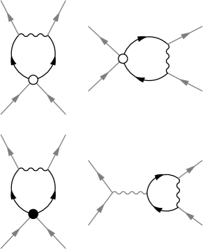
Figure 9: Additional one-loop diagrams contributing to the RG equations due to the nondiagonal part of the Green’s function.

Since $\mathcal{G}_{0,\alpha\beta}$ has become nondiagonal, there are new diagrams contributing to the renormalization of coupling constants. The new diagrams are illustrated in Fig. 9. In order to evaluate the angular integrals arising from DDI and nondiagonal Green’s function, we compute the RG equations only up to the linear order in $h_{0}$. This is a natural approximation, since we assume that initially $h_{0}$ is small if not vanishing. We analyze the accuracy of this approximation when we consider the fixed points corresponding to the full RG equations. The diagrams in Figs. 4, 8, and 9 yield the following contributions:

$$\mathrm{d}Z_{\eta}=\frac{4m}{15\pi\hbar^{2}}c_{\mathrm{dd}}(1+5\tilde{h}_{0})\chi_{0,1}\Lambda\mathrm{d}\ell,$$ (42)

$$\mathrm{d}h_{0}=\frac{2}{15\pi}c_{\mathrm{dd}}(3+5\tilde{h}_{0})\chi_{0,1}\Lambda\mathrm{d}\ell,$$ (43)

$$\mathrm{d}\mu=\big{[}-\frac{1}{3\pi^{2}}(g_{s}+2g_{d})(3+\tilde{h}_{0})+\frac{4}{3\pi}c_{\mathrm{dd}}\tilde{h}_{0}\big{]}\chi_{0,1}\Lambda^{3}\mathrm{d}\ell,$$ (44)

$$\mathrm{d}g_{s}=-\frac{1}{2\pi^{2}}\big{[}(3g_{s}^{2}+6g_{s}g_{d}-\delta_{1}c_{\mathrm{dd}}^{2})(1+2\tilde{h}_{0}/3)$$

$$\qquad\qquad+(\delta_{2}g_{s}c_{\mathrm{dd}}+\delta_{3}g_{d}c_{\mathrm{dd}}+\delta_{4}c_{\mathrm{dd}}^{2})\tilde{h}_{0}\big{]}\chi_{0,2}\Lambda^{3}\mathrm{d}\ell,$$ (45)

$$\mathrm{d}g_{d}=-\frac{1}{2\pi^{2}}\big{[}(5g_{d}^{2}+4g_{d}g_{s}+4g_{s}^{2}+\delta_{5}c_{\mathrm{dd}}^{2})(1+2\tilde{h}_{0}/3)$$

$$\qquad\qquad\qquad\qquad-(\delta_{6}g_{d}c_{\mathrm{dd}}+\delta_{7}c_{\mathrm{dd}}^{2})\tilde{h}_{0}\big{]}\chi_{0,2}\Lambda^{3}\mathrm{d}\ell,$$ (46)

$$\mathrm{d}c_{\mathrm{dd}}=-\frac{1}{2\pi^{2}}\big{[}(\delta_{8}c_{\mathrm{dd}}^{2}+2g_{d}c_{\mathrm{dd}}-4g_{s}c_{\mathrm{dd}})(1+2\tilde{h}_{0}/3)$$

$$\qquad\qquad\qquad\qquad\qquad\qquad-\delta_{9}c_{\mathrm{dd}}^{2}\tilde{h}_{0}\big{]}\chi_{0,2}\Lambda^{3}\mathrm{d}\ell,$$ (47)

where $\tilde{h}_{0}=h_{0}\Lambda^{2}/(\varepsilon_{\Lambda}-\mu)$ and $\chi_{0,n}=1/\beta(\varepsilon_{\Lambda}-\mu)^{n}$ for $n=1,2$. The numerical constants are given by $\delta_{1}=304\pi^{2}/45$, $\delta_{2}=16\pi/9$, $\delta_{3}=32\pi/9$, $\delta_{4}=128\pi^{2}/135$, $\delta_{5}=752\pi^{2}/45$, $\delta_{6}=2\delta_{3}$, $\delta_{7}=3\delta_{4}$, $\delta_{8}=8\pi/3$, and $\delta_{9}=\delta_{2}$. In the Zeeman basis, the full RG equations take the form

$$\frac{\mathrm{d}\ln Z_{\eta}}{\mathrm{d}\ell}=\frac{8\pi m}{15\hbar^{2}}c_{\mathrm{dd}}(1+5\tilde{h}_{0})K_{3}\Lambda\chi_{0,1},$$ (48)

$$\frac{\mathrm{d}h_{0}}{\mathrm{d}\ell}=-\eta h_{0}+\frac{4\pi}{15}c_{\mathrm{dd}}(3+5\tilde{h}_{0})K_{3}\Lambda\chi_{0,1},$$ (49)

$$\frac{\mathrm{d}\mu}{\mathrm{d}\ell}=(2-\eta)\mu-[\frac{2}{3}(c_{2}+2c_{0})(3+\tilde{h}_{0})$$

$$\hskip 119.50148pt-\alpha_{0}c_{\mathrm{dd}}\tilde{h}_{0}]K_{3}\Lambda^{3}\chi_{0,1},$$ (50)

$$\frac{\mathrm{d}c_{0}}{\mathrm{d}\ell}=(1-2\eta)c_{0}-[(5c_{0}^{2}+2c_{2}^{2}+\alpha_{1}c_{\mathrm{dd}}^{2})(1+\frac{2}{3}\tilde{h}_{0})$$

$$\hskip 27.03003pt-(\alpha_{2}c_{0}c_{\mathrm{dd}}+\alpha_{3}c_{2}c_{\mathrm{dd}}+\alpha_{4}c_{\mathrm{dd}}^{2})\tilde{h}_{0}]K_{3}\Lambda^{3}\chi_{0,2},$$ (51)

$$\frac{\mathrm{d}c_{2}}{\mathrm{d}\ell}=(1-2\eta)c_{2}-[(3c_{2}^{2}+6c_{0}c_{2}+\alpha_{5}c_{\mathrm{dd}}^{2})(1+\frac{2}{3}\tilde{h}_{0})$$

$$\hskip 27.03003pt-(\alpha_{6}c_{2}c_{\mathrm{dd}}+\alpha_{7}c_{0}c_{\mathrm{dd}}+\alpha_{8}c_{\mathrm{dd}}^{2})\tilde{h}_{0}]K_{3}\Lambda^{3}\chi_{0,2},$$ (52)

$$\frac{\mathrm{d}c_{\mathrm{dd}}}{\mathrm{d}\ell}=(1-2\eta)c_{\mathrm{dd}}-[(\alpha_{9}c_{\mathrm{dd}}^{2}+2c_{0}c_{\mathrm{dd}}+6c_{2}c_{\mathrm{dd}})$$

$$\hskip 65.44142pt\times(1+\frac{2}{3}\tilde{h}_{0})-\alpha_{10}c_{\mathrm{dd}}^{2}\tilde{h}_{0}]K_{3}\Lambda^{3}\chi_{0,2},$$ (53)

where we have defined the anomalous dimension as $\eta=d\ln Z_{\eta}/d\ell$. Comparison with Eqs. (20), (21), (25), and (26) shows that $\eta$ can be thought of as an effective correction to the spatial dimension of the system. Numerical constants $\alpha_{i}$ are defined as $\alpha_{0}=8\pi/3$, $\alpha_{1}=448\pi^{2}/45$, $\alpha_{2}=32\pi/9$, $\alpha_{3}=\alpha_{2}/2$, $\alpha_{4}=256\pi^{2}/135$, $\alpha_{5}=304\pi^{2}/45$, $\alpha_{6}=\alpha_{3}$, $\alpha_{7}=\alpha_{2}$, $\alpha_{8}=\alpha_{4}/2$, $\alpha_{9}=\alpha_{0}$, and $\alpha_{10}=\alpha_{3}$. The RG equations (48)–(VI) are computed up to the linear order $h_{0}$.

The fixed points corresponding to RG equations (48)–(VI) are shown in Table 3 where the dimensionless quantities are defined as $\hat{h}^{*}_{0}=\Lambda^{2}h_{0}^{*}/\varepsilon_{\Lambda}$, $\hat{\mu}^{*}=\mu^{*}/\varepsilon_{\Lambda}$ and $\hat{c}_{i}^{*}=\beta\varepsilon_{\Lambda}^{2}c_{i}^{*}/K_{3}\Lambda^{3}$. Table 3 shows that fixed points VII and VIII correspond to relatively large values of $\hat{h}_{0}$, and the original RG equations (48)–(VI) are no longer reliable in this region since they were calculated only up to the linear order in $h_{0}$. Linearized RG equations in the vicinity of fixed points V and VI give rise to complex eigenvalues. Similar behavior has been previously found in the context of dipolar ferromagnets with spatially uncorrelated disorder Aharony (1975) as well as in systems with long-range-correlated disorder Weinrib and Halperin (1983). We note that the appearance of complex eigenvalues for fixed points V and VI could be an artifact of our approximations, and therefore we concentrate on the properties of RG flows in the vicinity of fixed points I–IV where our calculation should capture the essential physics.

	I	II	III	IV	V	VI	VII	VIII
$\hat{h}_{0}^{*}$	$0$	$0$	$0$	$0$	$-0.355$	$-0.357$	$1.229$	$1.247$
$\hat{\mu}^{*}$	$0$	$0.250$	$0.250$	$0.286$	$0.282$	$0.279$	$0.204$	$0.124$
$\hat{c}_{0}^{*}$	$0$	$0.050$	$0.109$	$0.102$	$0.066$	$0.070$	$0.028$	$0.034$
$\hat{c}_{2}^{*}$	$0$	$0.088$	$-0.031$	$0$	$0.095$	$0.120$	$0.046$	$0.039$
$\hat{c}_{\mathrm{dd}}^{*}$	$0$	$0$	$0$	$0$	$0.007$	$-0.009$	$-0.002$	$0.009$
$\eta^{*}$	$0$	$0$	$0$	$0$	$-0.012$	$0.015$	$-0.015$	$0.068$

Table 3: Dimensionless values of the fixed points corresponding to RG equations (48)–(VI). All fixed points are unstable and linearized RG equations possess complex eigenvalues in the vicinity of fixed points V,VI, and VIII.

The Gaussian fixed point I is trivial since it is unstable to every direction in the space of the original coupling constants. Fixed points II–IV have certain common features such as the existence of one marginal scaling field arising from the combination of $h_{0}$ and $c_{\mathrm{dd}}$. This scaling field reflects the existence of a continuous line of fixed points for $c_{\mathrm{dd}}^{*}=0$, corresponding to an arbitrary value of $h_{0}^{*}$. Since $h_{0}$ was originally generated by DDI, we have taken $h_{0}^{*}=0$ for fixed points with $c_{\mathrm{dd}}^{*}=0$. Fixed points II–IV also have one scaling field directly proportional to $c_{\mathrm{dd}}$. This scaling field is irrelevant for fixed point II and relevant for fixed points III and IV.

To further analyze the behavior of RG flows in the case of weak DDI, we simplify the full RG equations by taking both $\mu$ and $h_{0}$ to be critical rg_ . This gives the reduced RG equations

$$\frac{dc_{0}}{d\ell}=(1-2\eta)c_{0}-(5c_{0}^{2}+2c_{2}^{2}+\alpha_{1}c_{\mathrm{dd}}^{2})\frac{K_{3}\Lambda^{3}}{\beta\varepsilon_{\Lambda}^{2}},$$ (54)

$$\frac{dc_{2}}{d\ell}=(1-2\eta)c_{2}-(3c_{2}^{2}+6c_{0}c_{2}+\alpha_{5}c_{\mathrm{dd}}^{2})\frac{K_{3}\Lambda^{3}}{\beta\varepsilon_{\Lambda}^{2}},$$ (55)

$$\frac{dc_{\mathrm{dd}}}{d\ell}=(1-2\eta)c_{\mathrm{dd}}-(\alpha_{9}c_{\mathrm{dd}}^{2}+2c_{0}c_{\mathrm{dd}}+6c_{2}c_{\mathrm{dd}})\frac{K_{3}\Lambda^{3}}{\beta\varepsilon_{\Lambda}^{2}},$$ (56)

where the anomalous dimension is given by $\eta=\frac{8\pi m}{15\hbar^{2}}c_{\mathrm{dd}}K_{3}/\beta\Lambda\varepsilon_{\Lambda}$. Apart from the anomalous dimension, the reduced RG equations are the same as Eqs. (35)–(37).

The reduced RG equations (54)–(56) can be used to justify the approximation of Sec. V, where the anomalous dimension was neglected altogether. Equations (54)–(56) have four fixed points I–IV shown in Table 2 corresponding to vanishing DDI (in 3D, we take $\epsilon=1$). In addition, there are two other non-trivial fixed points

$$\hat{c}_{0}^{*}=0.085,\,\,\,\hat{c}_{2}^{*}=0.114,\,\,\,\hat{c}_{\mathrm{dd}}^{*}=0.015,$$ (57)

$$\hat{c}_{0}^{*}=0.090,\,\,\,\hat{c}_{2}^{*}=0.150,\,\,\,\hat{c}_{\mathrm{dd}}^{*}=-0.008.$$ (58)

Comparing Eqs. (38) and (39) to Eqs. (57) and (58), one observes that the effect of anomalous dimension is negligible. Furthermore, Table 3 shows that the values of $\eta$ at fixed points are small compared to unity and hence the anomalous dimension has only a small effect on the fixed point structure of the full RG equations (48)–(VI).

In the vicinity of fixed points I–IV, linearized RG equations again give rise to one scaling field that is directly proportional to the dipole–dipole interaction. In the case of fixed points I, III, and IV, this scaling field is relevant and DDI introduces an additional instability. To quantify this instability, we define crossover exponents Ma (1976) $\phi_{i}=\lambda_{i}/\lambda_{\scriptscriptstyle\mathrm{DDI}}$, where $\lambda_{\scriptscriptstyle\mathrm{DDI}}$ is the eigenvalue corresponding to the DDI-induced scaling field and $\lambda_{1,2}$ are the two remaining eigenvalues corresponding to the flows depicted in Fig. 7. The crossover exponent $\phi_{i}$ indicates the relative importance of a given scaling field $s_{i}$ with respect to the DDI induced instability sca . When the absolute value of the crossover exponent becomes smaller than unity, the DDI-dependent instability dominates the RG flow with respect to $s_{i}$.

	I	II	III	IV
$\phi_{1}$	$1$	$5.498$	$-1.069$	$-1.667$
$\phi_{2}$	$1$	$-8.464$	$0.235$	$-0.333$

Table 4: Crossover exponents corresponding to fixed points I–IV in Table 2. For the fixed point II, we have replaced $\lambda_{\scriptscriptstyle\mathrm{DDI}}$ with $|\lambda_{\scriptscriptstyle\mathrm{DDI}}|$ since the DDI scaling field is irrelevant at fixed point II.

The crossover exponents are shown in Table 4 and they indicate that the properties of fixed point II are largely unaffected by the dipole–dipole interaction. On the other hand, fixed points I, II, and IV are susceptible to the runaway flows induced by DDI. To explore these runaway flows, we integrate the RG equations numerically in the vicinity of fixed points I–IV. We take $c_{dd}(0)$ to be small and positive, which is the physically relevant case. We find that the system exhibits the two runaway flows discussed in Sect. IV (see Fig 7). However, the mean-field regime governed by the fixed point IV becomes unstable and RG flows starting from this region correspond to the ferromagnetic runaway flow. The dipole–dipole interaction tends to increase under the ferromagnetic runaway flow, whereas under the antiferromagnetic runaway flow DDI renormalizes to zero. This is demonstrated in Figs. 10 and 11 where we show the sign of $c_{2}$ (Fig. 10) and the magnitude of $c_{\mathrm{dd}}$ (Fig. 11) in the asymptotic limit of RG flows. For each initial point $(\hat{c}_{0},\hat{c}_{2},\hat{c}_{\mathrm{dd}})$, we integrate the RG equations up to value $\ell_{c}$, where $\ell_{c}$ is given by the condition $|\hat{c}_{2}(\ell_{c})|=10$. Since both $\hat{c}_{0}$ and $\hat{c}_{2}$ diverge along the runaway flows, the precise value of $|\hat{c}_{2}(\ell_{c})|$ which determines $\ell_{c}$ is unimportant. It only needs to be large enough to illustrate the general tendency associated with the two runaway flows: for AFM runaway flow DDI renormalizes to zero whereas for FM runaway flow DDI tends to grow.

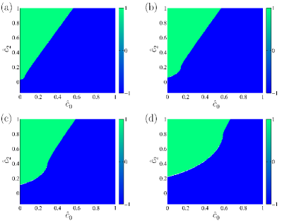
Figure 10: (Color online) Sign of the dimensionless coupling constant $\hat{c}_{2}(\ell_{c})$ for each initial point $(\hat{c}_{0},\hat{c}_{2},\hat{c}_{\mathrm{dd}})$. The dimensionless coupling constants are defined as $\hat{c}_{i}=\beta\varepsilon_{\Lambda}^{2}c_{i}/K_{D}\Lambda^{D}$, $i=0,2,\mathrm{dd}$. Reduced RG equations (54)–(56) are integrated up to $\ell_{c}$, where $\ell_{c}$ is determined by the condition $|\hat{c}_{2}(\ell_{c})|=10$. The initial values of $\hat{c}_{\mathrm{dd}}$ are (a) $\hat{c}_{\mathrm{dd}}(0)=0.01$, (b) $\hat{c}_{\mathrm{dd}}(0)=0.025$, (c) $\hat{c}_{\mathrm{dd}}(0)=0.05$, and (d) $\hat{c}_{\mathrm{dd}}(0)=0.1$.

Figures 10 and 11 demonstrate the existence of a phase transition separating an antiferromagnetic spin singlet condensate and a ferromagnetic condensate with anisotropic dipole–dipole interactions and suppressed fluctuations in the magnitude of local spin (dipolar ferromagnetic condensate). The dipole–dipole interaction favors spatial modulation in the local magnetization and in contrast to Sect. IV.2, the equilibrium phase corresponding to the ferromagnetic runaway does not feature all atoms in the same hyperfine spin state. Furthermore, even weak DDI renders antiferromagnetic and ferromagnetic condensates unstable towards formation of dipolar ferromagnetic condensate.

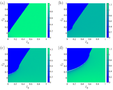
Figure 11: (Color online) Value of the dimensionless coupling constant $\hat{c}_{\mathrm{dd}}(\ell_{c})$ for different initial points $(\hat{c}_{0},\hat{c}_{2},\hat{c}_{\mathrm{dd}})$. The reduced RG equations are integrated up to $\ell_{c}$, where $\ell_{c}$ is determined by the condition $|\hat{c}_{2}(\ell_{c})|=10$. The initial values of $\hat{c}_{\mathrm{dd}}$ are the same as in Fig. 10, namely (a) $\hat{c}_{\mathrm{dd}}(0)=0.01$, (b) $\hat{c}_{\mathrm{dd}}(0)=0.025$, (c) $\hat{c}_{\mathrm{dd}}(0)=0.05$, and (d) $\hat{c}_{\mathrm{dd}}(0)=0.1$.

To verify that the anisotropic kinetic energy term represented by $h_{0}$ does not change the previous conclusions, we lift the assumption $h_{0}=0$ and integrate RG equations (48)–(VI) in the critical region corresponding $\mu=0$. We take $h_{0}$ initially zero since the original action does not contain the term in Eq. (27). We obtain RG flows identical to those depicted in Fig. 10 and 11. For the physically relevant case $c_{\mathrm{dd}}(0)>0$, we find that $h_{0}$ grows under both runaway flows. Under the antiferromagnetic runaway flow, the growth of $h_{0}$ is somewhat slower than in the case of ferromagnetic runaway flow.

We conclude this section by analysing the stability of the two additional fixed points given in Eqs. (57) and (58). As discussed in Sec. V.2, the RG flow in the vicinity of these new fixed points has somewhat unconventional properties that are similar to those discussed in Refs Aharony (1975); Weinrib and Halperin (1983). When the RG equations (54)–(56) are linearized in the vicinity of fixed points, the eigenvalues of the resulting matrix consist of one real eigenvalue and a pair of complex-conjugated eigenvalues in the case of physically relevant fixed point in Eq. (57). The real parts of eigenvalues determine the stability of the fixed point Weinrib and Halperin (1983), and we find that the fixed point in Eq. (57) is unstable and practically unattainable since the complex eigenvalues have positive real parts. Furthermore, RG flows near the fixed point in Eq. (57) are not markedly different from the RG flows near fixed points I–IV. We find that RG flows starting from positive $c_{\mathrm{dd}}$ remain positive and since the bare value of DDI coupling $c_{\mathrm{dd}}(0)=\mu_{0}\mu_{\scriptscriptstyle\mathrm{B}}^{2}g_{\scriptscriptstyle\mathrm{F}}^{2}/4\pi$ is positive, the fixed point in Eq. (58) corresponding to negative DDI coupling is not relevant for physical systems. For completeness, we note that linearized RG equations for the fixed point in Eq. (58) give rise to real eigenvalues, two of which are positive.

VII Effects associated with the anisotropic dispersion

To analyze the properties of the anisotropic kinetic energy term in Eq. (27), we restrict to the noninteracting limit and consider only the single-particle part $S_{0}+S_{0}^{\prime}$. Since the effects associated with dipole–dipole interactions become important only at finite temperatures, we neglect all nonzero Matsubara frequencies in the correlation function $G_{0,\alpha\beta}=\langle\psi_{\alpha}^{*}\psi_{\beta}\rangle$ and obtain

$$G_{0,\alpha\beta}(\bm{k})=\frac{1}{\varepsilon_{\bm{k}}-\mu}\big{(}\delta_{\alpha\beta}-\frac{k_{\alpha}k_{\beta}}{\bm{k}^{2}}\big{)}+\frac{1}{\varepsilon_{\bm{k}}-\mu-h_{0}\bm{k}^{2}}\frac{k_{\alpha}k_{\beta}}{\bm{k}^{2}}.$$ (59)

The anisotropic dispersion does not affect local spin order, but can nevertheless give rise to nematic order described by a tensor order parameter

$$(\mathcal{Q}_{s})_{\alpha\beta}=\frac{1}{2}(\psi_{\alpha}^{*}\psi_{\beta}+\psi_{\beta}^{*}\psi_{\alpha}).$$ (60)

Since we consider a uniform system with constant total density, our definition of $\mathcal{Q}_{s}$ is analogous to that of Ref. Mueller (2004).

In the non-interacting limit we have $\langle\mathcal{Q}_{s}(\bm{k})\rangle=G_{0,\alpha\beta}(\bm{k})$. The nematic order is associated with the eigenvalues and eigenvectors of $\langle\mathcal{Q}_{s}\rangle$. Following Ref. Mueller (2004), we define the nematic director $\hat{\bm{n}}$ to be the eigenvector corresponding to the largest eigenvalue of $\langle\mathcal{Q}_{s}\rangle$. Since $\langle\mathcal{Q}_{s}\rangle$ has to be positive semidefinite, we impose a condition $|h_{0}|<\hbar^{2}/2m$. This condition is also physically motivated since initially in the RG calculation, we assumed $h_{0}$ to be small compared to kinetic energy. Without losing generality we may also take $\mu=0$. For $h_{0}>0$ we obtain $\hat{\bm{n}}(\bm{k})=\hat{\bm{k}}$, corresponding to a hedgehog (monopole) in the momentum space. In the case $h_{0}<0$, there are two linearly independent nematic directors which can be taken to be $\hat{\bm{n}}_{1}(\bm{k})=(-k_{z},0,k_{x})/k_{xz}$ and $\hat{\bm{n}}_{2}(\bm{k})=(-k_{y},k_{x},0)/k_{xy}$, where $k_{x\alpha}=\sqrt{k_{x}^{2}+k_{\alpha}^{2}}$. Such nematic directors correspond to vortices in momentum space.

One of the experimental manifestations of dipolar interactions in spin-$1$ Bose gases is periodic spatial modulation in the local magnetization Vengalattore et al. (2010). Since we have considered only the noninteracting case in this section, the local spin order vanishes and our analysis cannot be directly compared with the experiment of Ref. Vengalattore et al. (2010). To study the nematic order associated with $h_{0}$ in real space, we Fourier transform $G_{0,\alpha\beta}$. The nematic director $\hat{\bm{n}}(\bm{r})$ corresponds to the hedgehog for $h_{0}<0$ and the two vortex solutions for $h_{0}>0$. Note that the hedgehog in real space corresponds to a vortex in momentum space and vice versa. The nematic ordering and the corresponding textures can in principle be measured in real space utilizing the atomic birefringence Carusotto and Mueller (2004); Higbie et al. (2005).

VIII Discussion

In this work, we have analyzed the properties of dipolar spin-$1$ Bose gases using momentum shell renormalization group and taking into account all one-loop diagrams. In the absence of magnetic dipole–dipole interactions, our RG analysis complements the previous RG studies of low-dimensional spinor Bose gases at $T=0$ Kolezhuk (2010) as well as the phenomenological analysis of Ref. Yang (2009). Similarly to Ref. Kolezhuk (2010), we found two runaway flows corresponding to the formation of either a condensate of spin singlet pairs or a fully spin-polarized scalar condensate. The absence of stable fixed points in the regions corresponding to runaway flows is sometimes a manifestation of a first-order transition Amit and Martín-Mayor (2005); Rudnick (1978). In the case of antiferromagnetic runaway flow, it would be interesting to study if stable fixed points arise when an additional field representing the spin singlet pairs is introduced Kolezhuk (2010). We believe that the possible first-order transition associated with the ferromagnetic runaway flow could be akin to the fluctuation-induced first-order transition in type I superconductors Halperin et al. (1974). For spinor Bose gases, the analogue of an intrinsic fluctuating magnetic field is given by the fluctuating Berry phase associated with the local magnetization Ho and Shenoy (1996).

In the zero-temperature limit, we found that the dipole–dipole interaction renormalizes to zero and does not induce any additional instabilities. At finite temperatures, we analyzed the limit where thermal fluctuations dominate quantum fluctuations. We found that the pair condensate is unaffected by the dipole–dipole interactions which eventually renormalize to zero. On the other hand, both antiferromagnetic and ferromagnetic condensates become unstable and the system exhibits an instability similar to the ferromagnetic runaway flow in the absence of DDI. In principle the magnetic dipole–dipole interaction can be transformed to an external vector potential such that the local spin of the gas $\bm{\mathcal{S}}$ couples linearly to the curl of the vector potential Belitz and Kirkpatrick (2010). This transformation gives rise to an alternative RG scheme which could provide further insight to the runaway flow induced by the DDI and its connection to the potential first-order transition. Also, the role of higher order terms beyond the one-loop approximation should be explored and one possible route to accomplish this task could be the functional renormalization group, from which the current RG equations arise in principle as an approximation Wetterich (1991); Andersen (2004).

Since the lifetime of ultracold atomic gases is limited and the spin–spin interactions are relatively weak, it is not clear to what extent the current experiments Vengalattore et al. (2008, 2010) are able to explore the true thermal equilibrium of the system. However, even if the experimentally attainable physics of spinor Bose gases eventually turns out to be inherently out of equilibrium, understanding the corresponding equilibrium systems is still a prerequisite for the exploration of the non-equilibrium situation. The experimentally relevant atomic species ²³Na and ⁸⁷Rb give rise to bare coupling constants that belong to the regions of antiferromagnetic and ferromagnetic condensates, respectively. In the absence of dipole–dipole interactions, the critical properties of both of these condensates are determined by the $SU(3)$-symmetric fixed point discussed in Section IV.2. When dipole–dipole interactions are taken into account, ferromagnetic and antiferromagnetic condensates become in principle unstable and the true equilibrium is determined by the ferromagnetic runaway flow. However, the lifetime of atomic gases can limit the possibilities of observing this crossover from the critical behavior determined by the non-dipolar fixed points of Sec. IV.2 and VI to the thermodynamic equilibrium determined by DDI.

Recently observed optical Feshbach resonances Hamley et al. (2009) as well as the proposed microwave induced Feshbach resonances Papoular et al. (2010) provide in principle means to fully explore the phase diagrams studied in this work. Alternatively, the phase diagrams in the absence of DDI could also be realized in the molecular superfluid phase of $p$-wave resonant Bose gases Radzihovsky and Choi (2009).