Systematic Uncertainties in the Spectroscopic Measurements of Neutron-Star Masses and Radii from Thermonuclear X-ray Bursts. I. Apparent Radii
Abstract
The masses and radii of low-magnetic field neutron stars can be measured by combining different observable quantities obtained from their X-ray spectra during thermonuclear X-ray bursts. One of these quantities is the apparent radius of each neutron star as inferred from the X-ray flux and spectral temperature measured during the cooling tails of bursts, when the thermonuclear flash is believed to have engulfed the entire star. In this paper, we analyze 13,095 X-ray spectra of 446 X-ray bursts observed from 12 sources in order to assess possible systematic effects in the measurements of the apparent radii of neutron stars. We first show that the vast majority of the observed X-ray spectra are consistent with blackbody functions to within a few percent. We find that most X-ray bursts follow a very well determined correlation between X-ray flux and temperature, which is consistent with the whole neutron-star surface emitting uniformly during the cooling tails. We develop a Bayesian Gaussian mixture algorithm to measure the apparent radii of the neutron stars in these sources, while detecting and excluding a small number of X-ray bursts that show irregular cooling behavior. This algorithm also provides us with a quantitative measure of the systematic uncertainties in the measurements. We find that those errors in the spectroscopic determination of neutron-star radii that are introduced by systematic effects in the cooling tails of X-ray bursts are in the range %. Such small errors are adequate to distinguish between different equations of state provided that uncertainties in the distance to each source and the absolute calibration of X-ray detectors do not dominate the error budget.
Subject headings:
stars: neutron — X-rays: bursts1. Introduction
The thermal spectra of neutron stars during thermonuclear X-ray bursts have been used during the last three decades in numerous attempts to measure the neutron-star masses and radii (e.g., van Paradijs 1978, 1979; Foster, Fabian & Ross 1986; Sztajno et al. 1987; van Paradijs & Lewin 1987; Damen et al. 1989, 1990). Such efforts were often hampered by large systematic uncertainties in the estimated distances to the bursters and in the theoretical models for their X-ray spectra. Moreover, the relatively small number of X-ray bursts observed by early satellites from each individual source made it impossible to assess systematic uncertainties related to the degree of anisotropy of the thermonuclear burning on the neutron-star surface, or of the obscuration by and the reflection off the accretion flow.
The situation has changed dramatically in the last few years. The distances to several globular clusters that contain bursting neutron stars has been narrowed down with the use of observations by the Hubble space telescope (see, e.g., Kuulkers et al. 2003; Özel, Güver, & Psaltis 2009; Güver et al. 2010b). The distances to X-ray bursters in the Galactic disk and halo have also been determined using alternate methods (e.g., Güver et al. 2010a). Theoretical models of the X-ray spectra of bursting neutron stars have been greatly improved and can account for the subtle effects of the presence of heavy metals in their atmospheres (e.g., London, Taam, & Howard 1986; Foster, Fabian, & Ross 1986; Ebisuzaki 1987; Madej, Joss, & Różańska 2004; Majczyna et al. 2005; Suleimanov, Poutanen, & Werner 2011). Finally, the high signal-to-noise observations of the X-ray spectra of several hundreds of bursts with the Rossi X-ray Timing Explorer (Galloway et al. 2008a) allow for the formal uncertainties of individual measurements to be substantially reduced.
The combination of these developments led recently to the measurement of the masses and radii of several neutron stars (Özel et al. 2009; Güver et al. 2010a, 2010b; Steiner, Lattimer, & Brown 2010) which are already sufficient to provide broad constraints on the equation of state of neutron-star matter (Özel, Baym, & Güver 2010). In some cases, the formal uncertainties in the spectroscopic measurements are as low as a few percent (Güver et al. 2010b) suggesting that their accuracy might be limited by systematic effects rather than by counting statistics.
In this series of articles, we use the large database of X-ray bursts observed with the RXTE in order to assess the systematic effects in various spectroscopic measurements of their properties. In the first article, we focus on the measurements of the apparent surface areas of 12 neutron stars as inferred from their X-ray spectra during the cooling tails of the bursts. Our goal is to quantify the degree to which: (i) the X-ray burst spectra observed in the RXTE energy range can be described by blackbody functions (the so-called color correction arising from atmospheric effects are then applied a posteriori); (ii) the entire surface area of each neutron star burns practically uniformly during the cooling of the bursts; (iii) the accretion flows make minor contributions to the emission during the bursts.
2. Sources, Observations, and Data Analysis
2.1. Source and Burst Selection
| Name | RA | DEC | Number | NH | NH |
|---|---|---|---|---|---|
| of Bursts | (1022 cm-2) | MethodaaReferences : (1) Harris 1996; (2) Güver et al. 2010a (3) Juett et al. (2004, 2006); (4) Wroblewski et al. 2008; (5) Wijnands et al. 2005; (6) Valenti et al. 2007; (7) Güver et al. 2010b; (8) Chevalier et al. 1999 | |||
| 4U 051340 | 05 14 06.60 | 40 02 37.0 | 6 | 0.0141 | GCbbOptical/IR observations of the globular cluster |
| 4U 160852 | 16 12 43.00 | 52 25 23.0 | 26 | 1.080.162 | X-ray edgesccHigh resolution spectroscopy of X-ray absorption edges |
| 4U 163653 | 16 40 55.50 | 53 45 05.0 | 162 | 0.443 | X-ray edgesccHigh resolution spectroscopy of X-ray absorption edges |
| 4U 1702429 | 17 06 15.31 | 43 02 08.7 | 46 | 1.95 | X-ray continuumddAverage of continuum X-ray spectroscopy |
| 4U 170544 | 17 08 54.47 | 44 06 07.4 | 44 | 2.440.094 | X-ray edgesccHigh resolution spectroscopy of X-ray absorption edges |
| 4U 1724307 | 17 27 33.20 | 30 48 07.0 | 3 | 1.081 | GCbbOptical/IR observations of the globular cluster |
| 4U 172834 | 17 31 57.40 | 33 50 05.0 | 90 | 2.49 0.144 | X-ray edgesccHigh resolution spectroscopy of X-ray absorption edges |
| KS 1731260 | 17 34 12.70 | 26 05 48.5 | 24 | 2.98 | X-ray continuumddAverage of continuum X-ray spectroscopy |
| 4U 173544 | 17 38 58.30 | 44 27 00.0 | 6 | 0.283 | X-ray edgesccHigh resolution spectroscopy of X-ray absorption edges |
| EXO 1745248 | 17 48 56.00 | 24 53 42.0 | 22 | 1.40.455 | X-ray continuumddAverage of continuum X-ray spectroscopy |
| 4U 174637 | 17 50 12.7 | 37 03 08.0 | 7 | 0.366 | GCbbOptical/IR observations of the globular cluster |
| SAX J1748.92021 | 17 48 52.16 | 20 21 32.4 | 4 | 0.796 | GCbbOptical/IR observations of the globular cluster |
| SAX J1750.82900 | 17 50 24.00 | 29 02 18.0 | 4 | 4.97 | X-ray continuumddAverage of continuum X-ray spectroscopy |
| 4U 182030 | 18 23 40.45 | 30 21 40.1 | 5 | 0.25 0.037 | X-ray edgesccHigh resolution spectroscopy of X-ray absorption edges |
| AQL X1 | 19 11 16.05 | 00 35 05.8 | 51 | 0.340.078 | CounterparteeOptical spectroscopy of the counterpart |
We base our study on the X-ray burst catalog of Galloway et al. (2008a). We chose 12 out of the 48 sources in the catalog based on the following criteria:
(i) We considered sources that show at least two bursts with evidence for photospheric radius expansion, based on the definition of the latter used by Galloway et al. (2008a). This requirement arises from our ultimate aim, which is to measure both the mass and the radius of the neutron star in each system using a combination of spectroscopic phenomena (as in, e.g., Özel et al. 2009).
(ii) We excluded dippers, ADC sources, or known high-inclination sources. This list includes EXO 0748676, MXB 1659298, 4U 191605, GRS 1747312, 4U 125469, and 4U 1710281, for which it was shown that geometric effects related to obscuration or reflection significantly affect the flux from the stellar surface that is measured by a distant observer (Galloway, Özel, & Psaltis 2008b).
(iii) We did not consider the known millisecond pulsars SAX J1808.43658 and HETE J1900.12455 because the presence of pulsations in their persistent emission implies that their magnetic fields are dynamically important and, therefore, may affect the properties of X-ray bursts.
(iv) We excluded the sources GRS 1741.92853 and 2E 1742.92929 as well as a small number of bursts from Aql X-1, 4U 172834, and 4U 174637, for which there is substantial evidence that their emission is affected by source confusion (Galloway et al. 2008a; Keek et al. 2010).
(v) For each source, we considered only bursts for which the flux in the persistent emission prior to the burst is at most 10% of the inferred Eddington flux for each source, i.e., , as calculated by Galloway et al. (2008a). Because we subtract the pre-burst persistent emission from the decay spectrum of each X-ray burst, this requirement reduces substantially the systematic uncertainties introduced by potential changes in the emission from the accretion flow during the burst.
Table 1 lists all the X-ray bursters that fulfill the above requirements, together with the number of bursts observed by RXTE for each source. This is the complete list of sources for which the masses and radii can be measured, in principle, using the spectroscopic method of Özel et al. (2009), with currently available data. Our analyses of the bursts from EXO 1745248, 4U 160852, and 4U 182030 have been reported elsewhere (Özel et al. 2009; Güver et al. 2010a, 2010b) and will not be repeated here.
2.2. Data Analysis
We analyzed the burst data for the 12 sources shown in Table 1 following the method outlined in Galloway et al. (2008a; see also Özel et al. 2009; Güver et al. 2010a, 2010b).
For each source, we extracted time resolved 2.525.0 keV X-ray spectra using the seextrct ftool for the science event mode data and the saextrct ftool for the science array mode data from all of the RXTE/PCA layers. Science mode observations provide high count-rate data with a nominal time resolution of 125s in 64 spectral channels over the whole energy range (260 keV) of the PCA detector. Following Galloway et al. 2008a, we extracted spectra integrated over 0.25, 0.5, 1, and 2 s time intervals, depending on the source count rate during the burst, so that the total number of counts in each spectrum is roughly constant. (In a few cases, data gaps during the observations result in X-ray spectra integrated over shorter exposure times). We took the spectrum over a 16 s time interval prior to the onset of each burst as the spectrum of the persistent emission, which we subtracted from the burst spectra as background.
We generated separate response matrix files for each burst using the PCARSP version 11.7, HEASOFT release 6.7, and HEASARC’s remote calibration database and took into account the offset pointing of the PCA during the creation of the response matrix files. This latest version of the PCA response matrix makes the instrument calibration self-consistent over the PCA lifetime and yields a normalization of the Crab pulsar that is within 1 of the calibration measurement of Toor & Seward (1974) for that source. In §4, we discuss in some detail the effect of the uncertainties in the absolute flux calibration on the measurement of the apparent surface area of neutron stars. Finally, we corrected all of the X-ray spectra for PCA deadtime following the method suggested by the RXTE team111ftp://legacy.gsfc.nasa.gov/xte/doc/cook_book/pca_deadtime.ps.
To analyze the spectra, we used the Interactive Spectral Interpretation System (ISIS), version 1.4.9-55 (Houck & Denicola 2000). For each fit, we included a systematic error of 0.5% as suggested by the RXTE calibration team222http://www.universe.nasa.gov/xrays/programs/rxte/pca/doc/rmf/pcarmf-11.7/.
We fit each spectrum with a blackbody function using the bbodyrad model (as defined in XSPEC, Arnaud 1996) and multiplied it by the tbabs model (Wilms, Allen, & McCray 2000) that takes into account the interstellar extinction, assuming ISM abundances. The model of the X-ray spectrum for each burst, therefore, depends on only three parameters: the color temperature of the blackbody, , the normalization of the blackbody spectrum, , and the equivalent hydrogen column density, of the interstellar extinction.
Allowing the hydrogen column density to be a free parameter in the fitting procedure leads to correlated uncertainties between the amount of interstellar extinction and the temperature of the blackbody. Moreover, for every 1022 cm-2 overestimation (underestimation) of the column density, the inferred flux of the thermal emission is systematically larger (smaller) by 10-9 erg cm-2 s-1 (Galloway et al. 2008a). Reducing the uncertainties related to the interstellar extinction for each burster is, therefore, very important in controlling systematic effects.
A recent analysis of high resolution grating spectra from a number of X-ray binaries (Miller, Cackett, & Reis 2009) showed that the individual photoelectric absorption edges observed in the X-ray spectra do not show significant variations with source luminosity or spectral state. This result strongly suggests that the neutral hydrogen column density is dominated by absorption in the interstellar medium and does not change on short timescales. In order to reduce this systematic uncertainty and given the fact that there is no evidence of variable neutral absorption for each system, we fixed the hydrogen column density for each source to a constant value that we obtained in one of the following ways. (i) For a number of sources, the equivalent hydrogen column density was inferred independently using high-resolution spectrographs. (ii) In cases where only an optical extinction or reddening measurement exists, we used the relation given by Güver & Özel (2009) to convert it to the equivalent hydrogen column density. (iii) Finally, for three sources (4U 1702429, KS 1731260, SAX J1750.82900) there are no independent hydrogen column density measurements published in the literature. In these cases, we fit the X-ray spectra obtained during all the X-ray bursts of each source allowing the NH value to vary in a wide range. We then found the resulting mean value of NH and used this as a constant in our second set of fits to all the X-ray bursts. In Table 1, we show the adopted values for the hydrogen column density together with the measurement uncertainties, the method with which the values were estimated, and the appropriate references. Future observations of these sources with X-ray grating spectrometers onboard Chandra and XMMNewton can help decrease the uncertainty arising from the lack of knowledge of the properties of the interstellar matter towards these sources.
Our goal in this article is to study potential systematic uncertainties in the measurement of the apparent area of each neutron star during the cooling tails of X-ray bursts. Hereafter, we adopt the following working definition of the cooling tail. It is the time interval during which the inferred flux is lower than the peak flux of the burst or the touchdown flux for photospheric radius expansion bursts. For the purpose of this definition, we use as a touchdown point the first moment at which the blackbody temperature reaches its highest value and the inferred apparent radius is lowest. In order to control the countrate statistics, we also set a lower limit on the thermal flux during each cooling tail of 510-9 erg s-1 cm-2 (or 510-10 for the exceptionally faint sources 4U 174637 and 4U 0513401).
In §3 and 4, we discuss in detail our approach of quantifying the systematic uncertainties in the measurements of the apparent radii during the cooling tails of thermonuclear bursts, using the sources KS 1731260, 4U 172834, and 4U 1636536 as case studies. For another analysis of the cooling tails of X-ray bursts from 4U 1636536, see Zhang, Mendez, & Altamirano (2011). In §5, we repeat this procedure systematically for seven additional sources from Table 1. Finally, the cooling tails of the bursts observed from 4U 051340 and Aql X-1 show irregular behavior, and we report our analysis of them in the Appendix.
3. Systematic Uncertainties in the Spectral Shapes
Our first working hypothesis is that the spectra of neutron stars during the cooling tails of thermonuclear bursts can be modeled by blackbody functions in the observed energy range. The fact that X-ray spectra can be described well with blackbody functions has been established since the first time resolved X-ray spectral studies of thermonuclear bursts (see, e.g., Swank et al. 1977; Lewin, van Paradijs, & Taam 1993; Galloway et al. 2008a and references therein). Under that assumption, the temperature measured by fitting blackbodies to the spectra are then corrected for the effects of the atmosphere by applying a numerical prefactor called the color correction factor , which is the ratio of the color to the effective temperature. This approach is expected to be only an approximation for a number of reasons.
First, theoretical models of the atmospheres of neutron stars in radiative equilibrium invariably show that the emerging spectra are broader than blackbodies, especially at low temperatures and towards low photon energies (e.g., Madej et al. 2004; Majczyna et al. 2005). Moreover, for neutron stars that are rapidly spinning, the spectra measured by an observer at infinity will be broader and more asymmetric with respect to those at the stellar surface (Özel & Psaltis 2003). The expected degree of broadening and asymmetry will be at most comparable to
| (1) |
where is the spin frequency of the neutron star and is its radius. This is an uncertainty that can, in principle, be corrected for by fitting the X-ray data with theoretical models of the X-ray spectra emerging from the atmospheres of rapidly spinning neutron stars.
Second, the accretion flow in the vicinity of the neutron star may alter in a number of ways the observed spectrum. It may act as a mirror, reflecting a fraction of the emerging radiation towards the observer and, therefore, increasing the apparent surface area of emission. It might occult a fraction of the stellar surface, reducing the apparent surface area of emission (see Galloway et al. 2008b). If the accretion flow is surrounded by a hot corona, Comptonization of the surface emission will alter its spectrum as well as the relation between energy flux and apparent surface area (e.g., Boutloukos, Miller, & Lamb 2010). Finally, the residual emission of the accretion flow, which we attempt to remove by subtracting the pre-burst spectrum of the source, might change during the duration of the burst, introducing systematic changes in the net spectrum.
All of the above effects have the potential of changing the shape of the X-ray spectrum of a burster and, perhaps more importantly, lead to stochastic changes in the inferred apparent radii. Their overall effect, however, is expected to be significantly reduced by the fact that the intense radiation field during each X-ray burst should either disrupt the inner accretion flow or cool any corona to the Compton temperature of the radiation. Such a phenomenon has been observed during a superburst from 4U 182030 (Ballantyne & Strohmayer 2004). Moreover, these effects are expected to be the strongest for high inclination systems (as was inferred by, e.g., Galloway et al. 2008b). This is why we not only limited our sample to bursts for which the ratio of the persistent flux prior to the burst to the Eddington flux in order to minimize accretion-related uncertainties but also selected the known high inclination sources out of our sample (see §2).

A final source of systematic uncertainties in the determination of the X-ray spectral shape of a burster is related to errors in the response matrix of the detector. These are expected to be %, according to the RXTE calibration team (see §2.2).
3.1. Goodness-of-fit Measures
In order to quantify the degree to which any of these effects influence the spectra of X-ray bursters, we fit all cooling-tail spectra from each source with a blackbody model, allowing for a level of systematic uncertainty , determined in the following way. We reduced the degree of freedom in this procedure by setting in each spectral bin to be a constant fraction of the Poisson error and fixed the value of to a constant for each source. We then added this systematic uncertainty to the formal Poisson error of each measurement in quadrature, i.e., , and defined a statistic such that
| (2) |
Here, is the standard statistic calculated for each fit. The posterior distribution of the new statistic may not be the same as that of the statistic and will depend on the nature of the systematic uncertainties. In order to explore the degree and nature of systematic uncertainties, we fit for each source the distribution with the distribution expected for the number of degrees of freedom used in the fits, with as a free parameter. Note that the expected distribution that we use is formally correct if the countrate data in the individual spectral bins have uncorrelated errors.
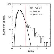
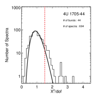
The expected and the observed distributions for the optimal value for KS 1731260, 4U 172834, and 4U 1636536 are shown in Figure 1. The value required to make the observed distributions for KS 1731260 consistent with the expected ones is 0.55 (see Table 2). This value corresponds to systematic uncertainties that are very small. As an example, we consider a typical 0.25 s integration for KS 1731260, when its spectrum is characterized by a color temperature of 2.5 keV. In this case, the average number of counts in each spectral bin in the 3-10 keV energy range is 110 ct and the corresponding Poisson uncertainty is %. Multiplying this by the inferred value for this source leads to the conclusion that the systematic uncertainties required to render the observed spectrum consistent with a blackbody are %. For the case of 4U 172834, which is brighter than KS 1731260, the formal uncertainties are % and the systematic uncertainties amount to %.
Figure 1 shows that the resulting distributions can be well approximated by the distribution but have weak tails extending to higher values. These tails most likely arise from the inconsistency of only a small number of spectra with blackbody functions even though we cannot rule out the possibility that the statistic follows a different posterior distribution than .
Figure 1 allows us also to identify the X-ray spectra that are statistically inconsistent with blackbodies. For each source, there is a maximum value of per degree of freedom beyond which the distribution of values deviates from the theoretical expectation. For the case of KS 1731260, this limiting value of the reduced is 1.7, for 4U 172834 it is 1.7, and for 4U 1636536 is 1.9 (see Table 2). The spectra with high reduced values often occur at the late stages of the cooling tails, where the subtraction of the persistent emission is the most problematic. However, unacceptable values may also be found in other, seemingly random places of the cooling tails. Nevertheless, the fraction of spectra that is inconsistent with blackbodies are %, %, and % for KS 1731260, for 4U 172834, and for 4U 1636536, respectively. Hereafter, we consider only the spectra that we regard to be statistically acceptable, given the values of the reduced .
| Source | Number of | /dof limitaafootnotemark: | Fraction of | |
|---|---|---|---|---|
| Spectra | Acceptable Spectra | |||
| 4U 051340 | 94 | 0.44 | 1.7 | 93.6% |
| 4U 163653 | 4579 | 0.59 | 1.9 | 99.3% |
| 4U 1702429 | 285 | 0.21 | 2.0 | 99.3% |
| 4U 170544 | 694 | bbfootnotemark: | 1.5 | 87.5% |
| 4U 1724307 | 58 | 0.44 | 1.5 | 91.4% |
| 4U 172834 | 2532 | 0.57 | 1.7 | 93.4% |
| KS 1731260 | 1312 | 0.52 | 1.7 | 98.2% |
| 4U 173544 | 40 | bbfootnotemark: | 2.0 | 97.5% |
| 4U 174637 | 187 | bbfootnotemark: | 1.6 | 85.0% |
| SAX J1748.92021 | 104 | 0.26 | 1.9 | 99.0% |
| SAX J1750.82900 | 82 | 0.54 | 1.7 | 100% |
| AQL X1 | 2191 | 0.45 | 1.6 | 92.1% |
| 11footnotetext: Maximum value of /dof beyond which we consider the blackbody fits of the spectra for each source to be statistically unacceptable. 22footnotetext: The distributions for these sources required no addition of systematic uncertainties. |
4. Systematic Uncertainties in the Inferred Emitting Area
Our second working hypothesis is that, during the cooling tail of each burst, the entire neutron star is emitting uniformly with negligible lateral temperature variations. This assumption is again expected to be violated at some level for a number of reasons. The non-uniformity of accretion onto the neutron star (e.g., Inogamov & Sunyaev 1999), the finite time of propagation of the burning front around the star (see, e.g., Nozakura, Ikeuchi, & Fujimoto 1984; Bildsten 1995; Spitkovsky, Levin, & Ushomirsky 2002), as well as the excitation of non-radial modes on the stellar surface (Heyl 2004; Piro & Bildsten 2005; Narayan & Cooper 2007) are all expected to lead to some variations in the effective temperature of emission at different latitudes and longitudes on the stellar surface.
The characteristics of burst oscillations observed during the cooling tails of X-ray bursts, however, imply that any variations in the surface temperatures of neutron stars can only be marginal. Indeed, any component of the variation in the surface temperature that is not symmetric with respect to the rotation axis leads to oscillations of the observed flux at the spin frequency of the neutron star. Such oscillations have been observed in the tails of bursts from many sources (Galloway et al. 2008a). The r.m.s. amplitudes of burst oscillations in the tails of bursts can be as large as 15%, although the typical amplitude is % (Muno, Özel, & Chakrabarty 2002). The stringent upper limits on the observed amplitudes at the harmonics of the spin frequencies can be accounted for only if the temperature anisotropies are dominated by the mode in which exactly half the neutron star is hotter than the other half (Muno et al. 2002). Moreover, the rather weak dependence of the r.m.s. amplitudes on photon energy (Muno, Özel, & Chakrabarty 2003) requires that any temperature variation between the hotter and cooler regions of the neutron star is keV, even for the bursts that show the largest burst oscillation amplitudes. All of the above strongly suggest that the expected flux anisotropy during the cooling tail of an X-ray burst is % and, therefore, the expected systematic uncertainties in the inferred apparent stellar radius will be half of that value, since the latter scales as the square root of the flux.
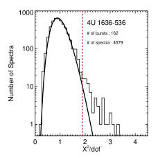
A final inherent systematic uncertainty in the spectroscopic measurement of the apparent surface area of a neutron star arises from the dependence of the color correction factor on the effective temperature of the atmosphere. In Figure 2 we show the predicted evolution of the color correction factor as a function of the color temperature of the spectrum as measured by an observer at infinity, for calculations by different groups for different neutron star surface gravities and atmospheric compositions (Madej et al. 2004; Majczyna et al. 2005; and Suleimanov et al. 2011). To make the models comparable to the observed evolution of the blackbody normalizations presented in the next section, we plot the color correction factor against the most directly observed quantity, i.e., the color temperature at infinity. When the color temperature at infinity is less than 2.5 keV, purely helium or low metallicity models show evolution of the color correction factor per keV of color temperature at infinity, while above 2.5 keV, they show an evolution of 1220% per keV. In contrast, solar metallicity models show a steady increase with color temperature in the keV range.111The color correction factor shows a turnover at different Eddington ratios and correspondingly at different color temperatures depending on composition, surface gravity, and gravitational redshift. The rapid evolution presented in Suleimanov et al. (2011) preferentially occurs at low Eddington ratios and color temperatures smaller than 1 keV (which we cannot explore observationally in the XTE burst data) and for very small surface gravities () which correspond only to neutron stars with radii km.
We infer the apparent surface area of a neutron star by measuring the X-ray flux and the color temperature at different intervals during the burst, so that
| (3) |
Here, is the Stefan-Boltzmann constant, is the distance to the source, and is the color correction factor. The value of the color correction factor is dictated by the predominant source of absorption and emission in the neutron-star atmosphere. It, therefore, depends on the effective temperature, which determines primarily the ionization levels, and on the effective gravitational acceleration, which determines the density profiles of the atmospheric layers. Both these quantities decrease as the cooling flux decreases. If we were to assume a constant value for the color correction factor, as it is customary, we would obtain a systematic change in the inferred apparent surface area as the cooling flux of the burst decreases with time. Such variations have been discussed in Damen et al. (1989) and in Bhattacharyya, Miller, & Galloway (2010). Note that this systematic effect can be corrected, in principle, if the data are fit directly with detailed models of neutron-star atmospheres (see, e.g., Majczyna & Madej 2005).
A potentially important source of uncertainty in the measurements is introduced by the errors in the absolute flux calibration of the RXTE/PCA detector. The current calibration of the PCA and the cross-calibration between X-ray satellites have been carried out using the Crab nebula as a standard candle (Jahoda et al. 2006; see also Toor & Seward 1974; Kirsch et al. 2005; Weisskopf et al. 2010). The uncertainties in the flux calibration can be due to a potential overall offset between the inferred and the true flux of the Crab nebula, which may be as large as 10% (Kirsch et al. 2005; Weisskopf et al. 2010). This can only change the mean value of the inferred apparent area in each source and does not alter the observed dispersion. We will explore this issue as well as uncertainties related to the variability of the Crab nebula itself (Wilson-Hodge et al. 2011) in more detail in Paper III of this series.
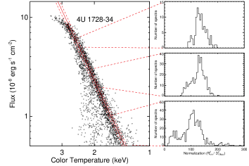
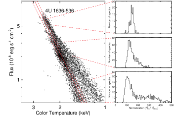
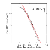
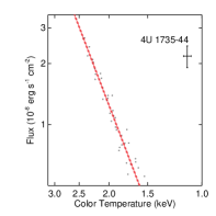
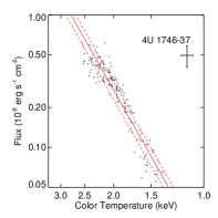
4.1. Flux-Temperature Diagrams
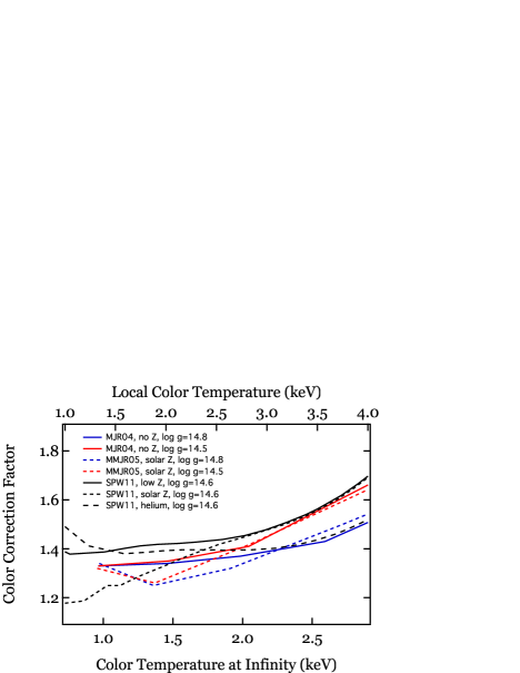
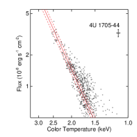
Figure 3 (left panels) show the dependence of the emerging flux on color temperature for all the spectra in the cooling tails of KS 1731260, 4U 172834, and 4U 1636536 that we consider to be statistically acceptable (see §3). We chose these three sources to use as detailed examples because of the high number spectra obtained for each and the fact that they span the range of behavior in cooling tracks that we will discuss below. If the whole neutron star is emitting as a single-temperature blackbody and the color correction factor is independent of color temperature, then should scale as . Our aim here is to investigate the systematic uncertainties on the measurement of the apparent surface area in each source at different flux levels. We, therefore, divided the data into a number of flux bins and plotted in the same figure (right panels) the distribution of the blackbody normalization values for some representative bins. The blackbody normalization for each spectrum is defined formally as , although in practice this is one of the two measured parameters and the flux is derived from the above definition. According to equation (3), the blackbody normalization is equal to and we report it in units of (km/10 kpc)2. If we do not correct for the dependence of the color correction factor on the flux, we expect the normalization to show a dependence on color temperature that is the mirror symmetric of that shown in Figure 2.
The flux-temperature diagrams of KS 1731260, 4U 172834, and 4U 1636536 share a number of similarities but are also distinguished by a number of differences. In all three cases, the vast majority of data points lie along a very well defined correlation. This reproducibility of the cooling curves of tens of X-ray bursts per source, combined with the lack of large amplitude flux oscillations during cooling tails of bursts, provides the strongest argument that the thermal emission engulfs the entire neutron-star surface with very small temperature variations at different latitudes and longitudes.
In 4U 172834, a deviation of the data points from the correlation is evident at high fluxes and color temperatures ( keV), which may be due to the evolution of the color correction factor at high Eddington fluxes (see the discussion in §4 and Fig. 2). The same deviation is not evident in KS 1731260 or 4U 1636536, for which the highest temperatures encountered in the cooling tails were keV.
Finally, in all three sources, a number of outliers exist at the lowest flux levels, with normalizations that deviate from the above correlation. In KS 1731260 and 4U 1636536, the outliers correspond to higher normalization values, whereas in 4U 172834 they correspond to lower normalization values with respect to the majority of the data points.
Any combination of the effects discussed earlier in this and in the previous section may be responsible for the outliers. Non-uniform cooling of the neutron star surface will lead to a reduced inferred value for the apparent surface area. Reflection of the surface X-ray emission off a geometrically thin accretion disk will cause an increase in the inferred value for the apparent surface area. Finally, Comptonization of the surface emission in a corona may have either effect, depending on the Compton temperature of the radiation.
Our goal in this work is not to understand the origin of the outliers, but rather to ensure that their presence does not introduce any biases in the measurements of the apparent surface areas inferred from the vast majority of spectra. Indeed, including the outliers in a formal fit of the flux-temperature correlation will cause a systematic increase of the apparent surface area with decreasing flux in KS 1731260 and in 4U 1636536 and a systematic decrease in 4U 172834 (c.f. Damen et al. 1990; Bhattacharyya et al. 2010). This issue was largely avoided in our earlier work (Özel et al. 2009; Güver et al. 2010a, 2010b) by considering only the relatively early time intervals in the cooling tail of each burst, which correspond only to the brightest flux bins. In order to go beyond this limitation here, we consider all spectral data for each burst and employ a Bayesian Gaussian mixture algorithm, which is a standard procedure for outlier detection in robust statistics (e.g., Titterington, Smith, & Makov 1985; McLachlan & Peel 2000; Huber & Ronchetti 2009).
Our working hypothesis that the main peak of normalizations in each flux interval corresponds to the signal and the remainder are outliers is shaped by two aspects of the observations. First, at high fluxes, each histogram can be described by a single Gaussian with no evidence or room for a second distribution of what we would call outliers. At lower fluxes, when the histograms can be decomposed into two Gaussians, the distribution with the highest peak has properties that smoothly connect to those of the single Gaussians at higher fluxes. Second, the Gaussians that we call our signal always contain the majority of the data points compared to the distribution of what we call the outliers. We take these as our criteria for defining our signal.
The algorithm, which we describe below in detail, allows us also to measure the degree of intrinsic variation in the apparent surface area for each source that is consistent with the width of the flux-temperature correlation. Even though we compare spectra in relatively narrow flux bins, the different observing modes as well as the different number of PCUs used in each observation result in a wide range of count rates and, hence, in a wide range of formal errors. This necessitates the use of the Bayesian approach we describe below as opposed to, e.g., performing fits of the distributions over blackbody normalization.
4.2. Quantifying Systematic Uncertainties with a Bayesian Gaussian Mixture Algorithm for Outlier Detection
Consider first the situation in which there are no systematic uncertainties and the inferred blackbody normalization from every spectrum reflects the apparent surface area of the entire neutron star. If this were the case, the intrinsic distribution of blackbody normalizations would be a delta function, while the observed distribution would be broader, with a width equal to the average formal uncertainties of the measurements.
In a more realistic situation, there is an intrinsic range of the inferred blackbody normalizations, caused by a combination of the various effects discussed earlier. We assume that, in each flux bin, the intrinsic distribution of normalization values is the Gaussian
| (4) |
where is its mean and is its standard deviation. The observed distribution of blackbody normalizations will be again broader than the intrinsic distribution because of the formal uncertainties in each measurement. Moreover, at low flux levels, a small number of outliers exists, which skews and introduces tails to the observed distribution. Our goal here is to quantify the most probable value of the blackbody normalization, i.e., the parameter in the distribution (4), as well as the intrinsic range of values in each flux bin, i.e., the parameter , while excluding the outliers.
When the inspection of an observed distribution requires an outlier detection scheme (as, e.g., in the lower right panels of Fig. 3), we model the distribution of outliers by a similar Gaussian, i.e.,
| (5) |
with a mean and a standard deviation . Our model distribution function is, therefore, in general the Gaussian mixture
| (6) |
where measures the relative fraction of outliers in our sample.
We are looking for the parameters in these distributions that maximize the posterior probability , which measures the likelihood that a particular set of parameters is consistent with the data. Using Bayes’ theorem, this probability distribution is
| (7) |
where is the posterior probability that the particular set of normalization data have been measured for a given set of parameters and the last five terms are the prior probabilities for the model parameters; the constant ensures that the probability density is normalized. We consider a flat prior probability distribution for the central value of each Gaussian in an interval that extends beyond the observed range of normalization values for each source. We also consider a flat prior probability distribution for the standard deviation for each Gaussian from (km/10 kpc)2 (which is practically zero) to a value equal to the width of the range of normalizations. Finally, we take a flat prior distribution of between zero and one. Our results are extremely weakly dependent on the ranges of parameter values we considered.
Given a set of observed normalization values and their uncertainties , we calculate the posterior probability of the data given a set of model parameters as
| (8) |
Here, is the value of each measurement and is its corresponding uncertainty, which we assume to be normally distributed; is a normalization constant. Using this posterior probability distribution, we identify the most probable values of the model parameters, as well as their uncertainties, following standard procedures.
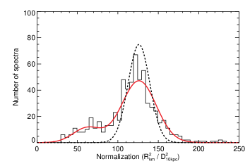
Figure 4 shows, as an example, the application of the Gaussian mixture algorithm to the distribution of blackbody normalizations obtained from fitting the spectra of 4U 172834, when the burst flux was in the range erg cm-2 s-1. The histogram shows the distribution of blackbody normalizations measured in this flux interval. The parameters of the Gaussian mixture that maximize the posterior probability distribution calculated using equation (7) correspond to an intrinsic distribution with a mean and standard deviation of (km/10 kpc)2 and (km/10 kpc)2, respectively, and a distribution of outliers with a mean of (km/10 kpc)2, a standard deviation of (km/10 kpc)2, and a relative normalization of . In order to compare the Gaussian mixture with the observed histogram, we first convolve it with a third Gaussian distribution with a standard deviation of (km/10 kpc)2 that is equal to the average formal errors of all measurements in this flux interval. The result is shown as a red solid line in Figure 4, which demonstrates that our assumption of a Gaussian distribution for the majority of the data and for the outliers is consistent with the observations.
We can appreciate the importance of excluding the outliers from the sample using the Bayesian Gaussian mixture algorithm in the following way. If we repeat the above procedure for the same flux interval in 4U 172834 but do not allow for the presence of outliers, the parameters of the intrinsic distribution will be (km/10 kpc)2 and (km/10 kpc)2, which are significantly different than the results quoted above. Moreover, had we assumed that there are no systematic errors but that the underlying distribution was a delta function, the most probable value would have been (km/10 kpc)2. The formal errors in such a measurement would have been substantially smaller compared to the systematic uncertainties.
In the following, we show in detail the application of this Gaussian mixture algorithm to all the flux intervals for the three sources.
| Flux interval ( erg s-1 cm-2) | |||||||||||
| Source | 0.5–1 | 1–2 | 2–3 | 3–4 | 4–5 | 5–6 | 6–7 | 7–8 | 8–9 | 9–10 | Averagebbfootnotemark: |
| 4U 1636536 | 112.6 | 124.6 | 126.9 | 142.7 | 144.2 | 145.7 | 145.7 | 149.5 | 130.7 | ||
| 18.7 | 16.1 | 12.4 | 22.4 | 18.4 | 15.1 | 14.1 | 4.6 | 20.9 | |||
| 4U 1702429 | 151.0 | 167.6 | 180.4 | 184.2 | 185.7 | 171.4 | 151.0 | 119.3 | 98.2 | 176.6 | |
| 13.9 | 10.1 | 9.9 | 4.1 | 3.9 | 8.1 | 8.1 | 17.2 | 12.4 | 11.6 | ||
| 4U 170544 | 80.2 | 86.9 | 86.9 | 82.4 | 83.9 | ||||||
| 9.9 | 7.1 | 10.9 | 7.4 | 9.1 | |||||||
| 4U 1724307 | 98.7 | 108.3 | 120.4 | 127.4 | 125.4 | 102.8 | 113.8 | ||||
| 7.1 | 4.6 | 12.6 | 3.7 | 19.4 | 15.4 | 15.4 | |||||
| 4U 172834 | 114.1 | 126.1 | 137.4 | 145.0 | 135.2 | 137.4 | 133.7 | 126.1 | 117.8 | 93.7 | 134.4 |
| 15.6 | 13.4 | 10.9 | 8.9 | 18.2 | 18.4 | 16.4 | 13.1 | 15.4 | 13.1 | 14.9 | |
| KS 1731260 | 72.6 | 89.9 | 93.0 | 95.2 | 95.2 | 96.0 | |||||
| 6.1 | 5.4 | 4.1 | 9.6 | 1.9 | 7.9 | ||||||
| 4U 173544 | 71.6 | 71.6ccfootnotemark: | 72.6ccfootnotemark: | 72.1ccfootnotemark: | |||||||
| 4.6 | |||||||||||
| 4U 174637ddfootnotemark: | 12.9 | 16.3 | 17.3 | 15.6 | 15.2 | 15.2 | 19.9 | 15.7 | |||
| 1.9 | 0.5 | 0.4 | 2.4 | 2.4 | 1.6 | 6.4 | 2.4 | ||||
| SAX J1748.92021 | 92.7 | 87.7 | 91.7 | 87.7 | 89.7 | ||||||
| 11.9 | 6.6 | 7.6 | 15.4 | 9.6 | |||||||
| SAX J1750.82900 | 126.9 | 110.8 | 106.8 | 97.2 | 86.2 | 93.2ccfootnotemark: | |||||
| 40.5 | 19.9 | 10.1 | 8.1 | 8.6 | 9.4 | ||||||
| 11footnotetext: The parameters of the intrinsic distribution of blackbody normalizations in different flux intervals for all the sources we considered in this manuscript. All normalizations are in units of (km/10 kpc)2. 22footnotetext: Taking into account all flux intervals for which the color temperature of the spectrum is keV; see text for details. 33footnotetext: The range of normalizations in this flux interval are consistent with no systematic uncertainties; the quoted uncertainties are purely statistical. 44footnotetext: For 4U 174637, all flux intervals are in units of erg s-1 cm-2. | |||||||||||
| Source | Rkm / D10kpc |
|---|---|
| 4U 163653 | 11.4 1.0 |
| 4U 1702429 | 13.3 0.4 |
| 4U 170544 | 9.2 0.5 |
| 4U 1724307 | 10.7 0.7 |
| 4U 172834 | 11.6 0.7 |
| KS 1731260 | 9.8 0.4 |
| 4U 173544 | 8.5 |
| 4U 174637 | 4.0 0.3 |
| SAX J1748.92021 | 9.5 0.5 |
| SAX J1750.82900 | 9.6 0.5 |
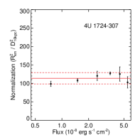
4.3. Dependence of Blackbody Normalizations on X-ray Flux
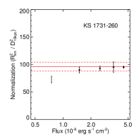
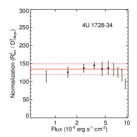
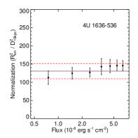
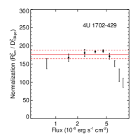
Figure 5 shows the result of the outlier detection procedure as applied to the various flux intervals of KS 1731260, 4U 172835, and 4U 1636536 (see also Table 3). Each dot represents the most likely centroid of the intrinsic distribution of blackbody normalizations, while each error bar represents its most likely width.
The normalization of the blackbody in the case of 4U 172834 shows a strong dependence on flux when the source is emitting at near-Eddington rates. This is not seen in KS 1731260 and 4U 1636536, for which the color temperature never reached temperatures above 2.5 keV. In fact, in our observed sample, the strong dependence of the normalization on the flux is seen in all three sources with color temperatures in excess of 2.5 keV, namely 4U 172834, 4U 1702429, and 4U 1724307 (see Fig. 6 below) but is absent from the other sources. The evolution of the blackbody normalization at near-Eddington fluxes depends on the local gravitational acceleration () on the neutron-star surface and on its composition. Therefore, modeling the decline of the blackbody normalization at large fluxes would allow us, in principle, to measure the combination of the mass and radius of the neutron star, as has been attempted by Majczyna & Madej (2005) and by Suleimanov et al. (2011).

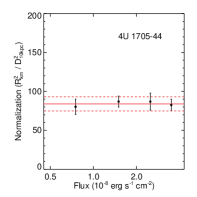


At low burst fluxes, the observed normalizations show a small albeit statistically significant trend towards lower values. In the case of 4U 172834, where the potential decrease is the largest, the normalization changed from (km/10 kpc)2 to (km/10 kpc)2 as the flux declined from erg s-1 cm-2 to erg s-1 cm-2. This corresponds to a % reduction in the normalization. In other sources, the decline is even smaller. This weak dependence seen in the data argues against the models with solar composition, as shown in Figure 2.
The decline in the normalization can, in principle, be accounted for with a % increase in the color correction factor (see eq. [3]) towards low temperatures. As can be seen in Figure 2, current atmosphere models do not predict such an evolution. However, as we discussed in the beginning of §4, a number of effects related to the physics of bursts on the neutron star surface (uneven cooling and burst oscillations), as well as the reduced sensitivity of the PCA at low energies, are capable of causing the observed trend in the normalization. Moreover, the effect in the data we would aim to model is comparable to the uncertainty in inferring theoretically the color correction factor from the atmosphere models and is also comparable to the deviation of the observed and theoretical spectra from blackbodies. The latter concern can be remedied by fitting directly theoretical model spectra to the data, but reducing the theoretical uncertainties present in the models to less than few percent is significantly more challenging.
An alternative approach is to allow for a range of values for the color correction factor that span the spread of theoretical uncertainties, metallicities, and fluxes of the cooling tails. In earlier work (Güver et al. 2010a, 2010b) we allowed for a 7% range in the color correction factor (from 1.3 to 1.4), which is adequate to account for the evolution in the blackbody normalizations shown by the data. Following this approach, we need to identify the range of blackbody normalizations we obtained from the data at different flux intervals as a systematic uncertainty in the measurement. In order to achieve this, we applied the Bayesian Gaussian mixture algorithm to the combined data set for each source for all flux intervals that correspond to a color temperature keV. This way, we computed the most probable value for the blackbody normalization for each source in a wide flux range as well as the systematic uncertainties in that measurement, which account for the potential decline of the normalization with decreasing flux.
In Figure 5, we identify the flux intervals we used for each source with a filled circle in the middle of each error bar. We also depict with a solid line the most probable value of the normalization in this wide flux range and with dashed lines the range of systematic uncertainties. Our results are summarized in Table 3. The blackbody normalizations for KS 1731260, 4U 172834, and 4U 1636536 are 96.07.9 (km/10 kpc)2, 134.414.9 (km/10 kpc)2, and 130.720.9 (km/10 kpc)2, respectively, with the uncertainties dominated entirely by systematics.
5. The Apparent Radii of X-ray Bursters
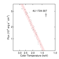
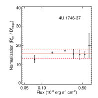
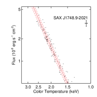
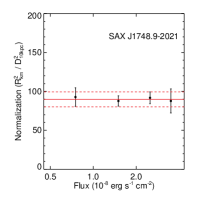
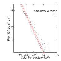
Figures 6–8 and Tables 2–3 show the results obtained after applying the procedure outlined in §4 to seven more sources from Table 1. The last two sources, 4U 051340 and Aql X-1 show large variations in the cooling tails of individual bursts and are discussed in detail in the Appendix. Moreover, in the Appendix we also discuss a number of bursts from 4U 1702429 and a long burst from 4U 1724307, which we did not include in the analysis.
As in the case of the three sources discussed in the previous section, the vast majority of the spectra observed during the cooling tails of X-ray bursts are very well described by blackbody functions, with only marginal allowance for systematic variations. In the flux-temperature diagrams, the cooling tails largely follow a well defined and reproducible track. Finally, in each flux interval of most sources, the range of blackbody normalizations obtained from a large number of bursts is consistent with a small degree of systematic uncertainties.
The measurements of the average blackbody normalizations in all sources are dominated by systematic uncertainties (the main exception is 4U 173544). However, these uncertainties are small, ranging from % in the case of 4U 1702429 to % in the case of 4U 1636536. The apparent radius of each neutron star scales as the square root of the blackbody normalization. As a result, the errors in the spectroscopic determination of neutron-star radii introduced by systematic effects in the cooling tails of X-ray bursts are in the range % (see Table LABEL:radii_table). Such small errors by themselves do not preclude distinguishing between different equations of state of neutron-star matter.


Appendix A 4U 1702429
A total of 46 bursts have been observed from the source 4U 1702429. Six of these bursts reach high fluxes and have been categorized as Photospheric Radius Expansion bursts by Galloway et al. (2008a). The remaining 40 bursts typically reach lower fluxes. In the main body of this paper, we focused on the 6 bright bursts from this source and exclude the remaining for two reasons that we explore in this appendix.
The left panel of Figure 9 shows the histogram of /dof values for the 880 spectra observed during the cooling tails of the 40 bursts and compares them to the expected distribution given the number of degrees of freedom. It is evident that blackbody functions provide statistically unacceptable fits to the majority of the spectra.
Had we not considered these spectra unacceptable, we would find that, approximately 4 seconds after the bursts start, the inferred blackbody normalizations increase rapidly to large values. The increase in normalization is, in fact, correlated with an increase in the /dof values, as shown in the right panel of Figure 9, rendering them even more suspect. These two arguments strongly suggest that the spectra of the 40 weak X-ray bursts from 4U 1702429 are not dominated by the thermal emission from the neutron star.
Appendix B 4U 1724307
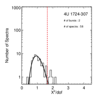
The first X-ray burst observed from 4U 1724307 on 1996 November 08 during observation 10090-01-01-02 is very different compared to the other two X-ray bursts that we used in the main text. The first burst is unusually long ( s), while the other two bursts are much shorter ( s range, as is typical for the vast majority of the Type-I bursts observed). Moreover, while the spectra of the short bursts are accurately modeled with blackbody functions (see top panels of Fig. 6), fitting the spectra during the cooling tail of the long burst results in unacceptably large values of /dof and the distritubiton of the resulting /dof values do not follow the expected distribution (see left panel of Fig. 10). Adding a certain amount of systematic uncertainty to the data can in principle result in a decrease in the individual /dof values; however,it can not change the fact that the resulting /dof distribution does not follow the expected distribution.
If we went ahead and further analyzed these statistically unacceptable spectra, we would have obtained values for the blackbody normalization that are larger compared to those of the shorter bursts (see right panel of Fig. 10).
The large values and the seemingly random distribution of /dof suggest that the X-ray spectra in the cooling tail of the long burst from 4U 1724307 are not dominated by the thermal emission from the neutron star. In fact, in’t Zand & Weinberg (2010) found evidence for atomic edges and a reflection component in the spectra of this burst, which they attributed to the presence of heavy metals in the ashes of previous bursts that were exposed by the long radius-expansion episode. For these reasons, we excluded the long X-ray burst observed from 4U 1724307 from our analysis. Note that Suleimanov et al. (2011) chose the spectra from this burst in order to infer the mass and radius of the neutron star in 4U 1724307. Had they chosen the other two bursts from the same source, the spectra of which are actually well described by blackbody functions, they would have obtained a radius of the neutron star that is % smaller, making their result consistent with the radii inferred for the other sources using this method (Özel et al. 2009; Güver et al. 2010a, 2010b) as well as with radii inferred from quiescent neutron stars in globular clusters (e.g., Webb & Barret 2007; Guillot, Rutledge, & Brown 2010).
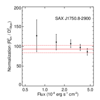
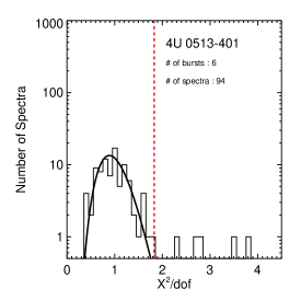
Appendix C 4U 051340
Six bursts have been observed from the source 4U 051340. While most of the X-ray spectra during the cooling tails of these bursts can be described well by blackbody functions (left panel of Fig. 11), the flux-temperature diagrams show irregular behaviour for the cooling tails (right panel of Fig. 11). In particular, two of the bursts show a cooling tail that is reminiscent of the long burst from 4U 1724307 discussed above: early in the cooling phase the temperature of the blackbody decreases while the flux remains constant and, when the flux starts decreasing, the cooling occurs with blackbody normalizations that are on average larger compared to the other bursts.
It is plausible that the spectra of these bursts from 4U 051340 are also affected by the presence of atomic lines, but the relatively low flux of 4U 051340 (which is a factor of smaller compared to that of 4U 1724307 at similar temperatures) still allows us to fit the observed spectra with blackbody functions. We do not consider this source suitable for a radius measurement based on the burst data.

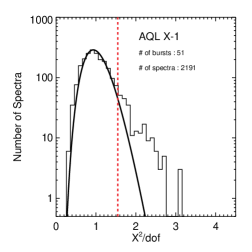
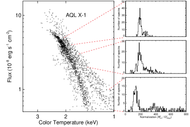
Appendix D Aql X-1
The transient source Aql X-1 has shown 51 X-ray bursts, from which we extracted 2191 spectra. Most of these spectra are well fit by blackbody functions, but their cooling tracks in the flux-temperature diagram depend strongly on the properties of the bursts (see Fig. 12). In particular, a large number of bursts are relatively short and reach modest fluxes (typically erg s-1 cm-2) with cooling tracks in the flux-temperature diagram that are reproducible. On the other hand, many bursts, which are relatively longer, reach fluxes that are a factor of higher, are often characterized by radius expansion episodes, and follow a range of cooling tracks in the flux-temperature diagram with blackbody normalizations that are typically larger than those of the other bursts.
One plausible exlanation is related to the fraction of the neutron star surface that is engulfed by the thermonuclear flash. In weak flashes, the burning front may not propage across the entire surface and, therefore, only a fraction of the stellar surface contributes to the normalization of the blackbody. On the other hand, in stronger flashes, a larger fraction of the neutron star surface is covered.
The source Aql X-1 is one of the two main examples (the other being the source 4U 1636536) discussed by Bhattacharrya et al. (2010) as evidence for systematic variations in the burning area during thermonuclear X-ray bursts. It is important to emphasize here, however, that the case of Aql X-1 is very unusual compared to the remaining sources that we analyzed and is, perhaps, related to the presence of a weak but dynamically important magnetic field in this source, as inferred from the observation of intermittent persistent pulsations (Casella et al. 2008).
References
- (1) Arnaud, K. A. 1996, in Astronomical Society of the Pacific Conference Series, Vol. 101, Astronomical Data Analysis Software and Systems V, ed. G. H. Jacoby & J. Barnes, 17–+
- (2) Ballantyne, D. R., & Strohmayer, T. E. 2004, ApJ, 602, L105
- (3) Bhattacharyya, S., Miller, M. C., & Galloway, D. K. 2010, MNRAS, 401, 2
- (4) Bildsten, L. 1995, ApJ, 438, 852
- (5) Boutloukos, S., Miller, M. C., & Lamb, F. K. 2010, ApJ, 720, L15
- (6) Casella, P., Altamirano, D., Patruno, A., Wijnands, R., & van der Klis, M. 2008, ApJ, 674, L41
- (7) Chevalier, C., Ilovaisky, S. A., Leisy, P., & Patat, F. 1999, A&A, 347, L51
- (8) Damen, E., Jansen, F., Penninx, W., Oosterbroek, T., van Paradijs, J., & Lewin, H. G. 1989, MNRAS, 237, 523
- (9) Damen, E., Magnier, E., Lewin, W. H. G., Tan, J., Penninx, W., & van Paradijs, J. 1990, A&A, 237, 103
- (10) Ebisuzaki, T. 1987, PASJ, 39, 287
- (11) Foster, A. J., Fabian, A. C., & Ross, R. R. 1986, MNRAS, 221, 409
- (12) Galloway, D. K., Muno, M. P., Hartman, J. M., Psaltis, D., & Chakrabarty, D. 2008a, ApJS, 179, 36
- (13) Galloway, D. K., Özel, F., & Psaltis, D. 2008b, MNRAS, 387, 268
- (14) Guillot, S., Rutledge, R. E., & Brown, E. F. 2010, arXiv:1007.2415
- Güver Özel (2009) Güver, T., Özel, F. 2009, MNRAS, 400, 2050
- (16) Güver, T., Özel, F., Cabrera-Lavers, A., & Wroblewski, P. 2010a, ApJ, 712, 964
- Güver et al. (2010) Güver, T., Wroblewski, P., Camarota, L., Özel, F. 2010b, ApJ, 719, 1807
- (18) Harris, W. E. 1996, AJ, 112, 1487
- (19) Heyl, J. S. 2004, ApJ, 600, 939
- (20) Houck, J. C., & Denicola, L. A. 2000, in Astronomical Society of the Pacific Conference Series, Vol. 216, Astronomical Data Analysis Software and Systems IX, ed. N. Manset, C. Veillet, & D. Crabtree, 591–+
- (21) Huber, P.J̇., & Ronchetti, E. M. 2009, Robust Statistics (Wiley)
- (22) in ’t Zand, J. J. M., & Weinberg, N. N. 2010, arXiv:1001.0900
- (23) Inogamov, N. A., & Sunyaev, R. A. 1999, Astronomy Letters, 25, 269
- (24) Jahoda, K., Markwardt, C. B., Radeva, Y., Rots, A. H., Stark, M. J., Swank, J. H., Strohmayer, T. E., & Zhang, W. 2006, ApJS, 163, 401
- (25) Juett, A. M., Schulz, N. S., & Chakrabarty, D. 2004, ApJ, 612, 308
- (26) Juett, A. M., Schulz, N. S., Chakrabarty, D., & Gorczyca, T. W. 2006, ApJ, 648, 1066
- (27) Keek, L., Galloway, D. K., in’t Zand, J. J. M., & Heger, A. 2010, ApJ, 718, 292
- Kirsch et al. (2005) Kirsch, M. G., et al. 2005, Proc. SPIE, 5898, 22
- (29) Kuulkers, E., den Hartog, P. R., in’t Zand, J. J. M., Verbunt, F. W. M., Harris, W. E., & Cocchi, M. 2003, A&A, 399, 663
- Lewin et al. (1993) Lewin, W. H. G., van Paradijs, J., & Taam, R. E. 1993, Space Sci. Rev., 62, 223
- (31) London, R. A., Taam, R. E., & Howard, W. M. 1986, ApJ, 306, 170
- (32) Madej, J., Joss, P. C., & Różańska, A. 2004, ApJ, 602, 904
- (33) Majczyna, A., & Madej, J. 2005, Acta Astronomica, 55, 349
- (34) Majczyna, A., Madej, J., Joss, P. C., & Różańska, A. 2005, A&A, 430, 643
- (35) McLachlan, G., Peel, D. 2000, Finite Mixture Models (Wiley)
- (36) Miller, J. M., Cackett, E. M., & Reis, R. C. 2009, ApJ, 707, L77
- (37) Muno, M. P., Özel, F., & Chakrabarty, D. 2002, ApJ, 581, 550
- (38) Muno, M. P., Özel, F., & Chakrabarty, D. 2003, ApJ, 595, 1066
- (39) Narayan, R., & Cooper, R. L. 2007, ApJ, 665, 628
- (40) Nozakura, T., Ikeuchi, S., & Fujimoto, M. Y. 1984, ApJ, 286, 221
- Özel et al. (2010) Özel, F., Baym, G., Güver, T. 2010, Phys. Rev. D, 82, 101301
- (42) Özel, F., Güver, T., & Psaltis, D. 2009, ApJ, 693, 1775
- (43) Özel, F., & Psaltis, D. 2003, ApJ, 582, L31
- (44) Piro, A. L., & Bildsten, L. 2005, ApJ, 629, 438
- (45) Spitkovsky, A., Levin, Y., & Ushomirsky, G. 2002, ApJ, 566, 1018
- Steiner et al. (2010) Steiner, A. W., Lattimer, J. M., & Brown, E. F. 2010, ApJ, 722, 33
- (47) Suleimanov, V., Poutanen, J., Revnivtsev, M., & Werner, K. 2010, arXiv:1004.4871
- Suleimanov et al. (2011) Suleimanov, V., Poutanen, J., & Werner, K. 2011, A&A, 527, A139
- (49) Sztajno, M., Fujimoto, M. Y., van Paradijs, J., Vacca, W. D., Lewin, W. H. G., Penninx, W., & Trumper, J. 1987, MNRAS, 226, 39
- Swank et al. (1977) Swank, J. H., Becker, R. H., Boldt, E. A., Holt, S. S., Pravdo, S. H., & Serlemitsos, P. J. 1977, ApJ, 212, L73
- (51) Titterington, D. M., Smith, A. F. M, Makov U. E., 1985, Statistical Analysis of Finite Mixture Distributions (John Wiley & Sons)
- (52) Toor, A., & Seward, F. D. 1974, AJ, 79, 995
- (53) Valenti, E., Ferraro, F. R., & Origlia, L. 2007, AJ, 133, 1287
- van Paradijs (1979) van Paradijs, J. 1979, ApJ, 234, 609
- van Paradijs (1978) van Paradijs, J. 1978, Nature, 274, 650
- (56) van Paradijs, J., & Lewin, W. H. G. 1987, A&A, 172, L20
- (57) Webb, N. A., & Barret, D. 2007, ApJ, 671, 727
- Weisskopf et al. (2010) Weisskopf, M. C., Guainazzi, M., Jahoda, K., Shaposhnikov, N., O’Dell, S. L., Zavlin, V. E., Wilson-Hodge, C., & Elsner, R. F. 2010, ApJ, 713, 912
- (59) Wijnands, R., Heinke, C. O., Pooley, D., Edmonds, P. D., Lewin, W. H. G., Grindlay, J. E., Jonker, P. G., & Miller, J. M. 2005, ApJ, 618, 883
- (60) Wilms, J., Allen, A., & McCray, R. 2000, ApJ, 542, 914
- (61) Wilson-Hodge, C. A., et al. 2011, ApJ, 727, L40
- (62) Wroblewski, P., Güver, T., & Özel, F. 2008, arXiv:0810.0007
- Zhang et al. (2011) Zhang, G., Méndez, M., & Altamirano, D. 2011, MNRAS, 413, 1913