A fully relativistic twisted disc around a slowly rotating Kerr black hole: derivation of dynamical equations and the shape of stationary configurations

Abstract

In this paper we derive equations describing dynamics and stationary configurations of a twisted fully relativistic thin accretion disc around a slowly rotating black hole. We assume that the inclination angle of the disc is small and that the standard relativistic generalisation of the $\alpha$ model of accretion discs is valid when the disc is flat. We find that similarly to the case of non-relativistic twisted discs the disc dynamics and stationary shapes can be determined by a pair of equations formulated for two complex variables describing orientation of the disc rings and velocity perturbations induced by the twist.

We analyse analytically and numerically the shapes of stationary twisted configurations of accretion discs having non-zero inclinations with respect to the black hole equatorial plane at large distances $r$ from the black hole. It is shown that the stationary configurations depend on two parameters - the viscosity parameter $\alpha$ and the parameter $\tilde{\delta}=\delta_{*}/\sqrt{a}$, where $\delta_{*}$ is the opening angle ($\delta_{*}\sim h/r$, where $h$ is the disc half thickness and $r$ is large) of a flat disc and $a$ is the black hole rotational parameter. When $a>0$ and $\tilde{\delta}\ll 1$ the shapes depend drastically on value of $\alpha$. When $\alpha$ is small the disc inclination angle oscillates with radius with amplitude and radial frequency of the oscillations dramatically increasing towards the last stable orbit, $R_{ms}$. When $\alpha$ has a moderately small value the oscillations do not take place but the disc does not align with the equatorial plane at small radii. The disc inclination angle is either increasing towards $R_{ms}$ or exhibits a non-monotonic dependence on the radial coordinate. Finally, when $\alpha$ is sufficiently large the disc aligns with the equatorial plane at small radii. When $a<0$ the disc aligns with the equatorial plane for all values of $\alpha$.

The results reported here may have implications for determining structure and variability of accretion discs close to $R_{ms}$ as well as for modelling of emission spectra coming from different sources, which are supposed to contain black holes.

1 Introduction

Twisted accretion discs around rotating black holes are used for explanations of different observational phenomena. For example they are invoked to explain jet precession observed in certain active galactic nuclei (AGN) (e.g. Caproni, Mosquera Cuesta & Abraham (2004) and references therein ), warping of the accretion disc in the maser galaxy NGC 4258 (e.g. Papaloizou, Terquem & Lin (1998); Caproni et al. (2007); Martin (2008)), certain features of emission line profiles coming from AGN (e.g. Bachev (1999); Cadez et al. (2003); Wu, Chen & Yuan (2010)) etc.. Ferreira & Ogilvie (2008, 2009) proposed that shear velocities induced by the disc twist (see below) provide a mechanism of excitation of high frequency quasi-periodic oscillations observed in many astronomical objects. Light curves, forms of emission lines of precessing twisted tori around a Kerr black hole as well as their shapes as seen from large distances have recently been investigated numerically by Dexter & Fragile (2011).

Theoretical studies of thin twisted discs started from the seminal paper Bardeen & Petterson (1975), who proposed a simple model of a stationary twisted disc, where a twisted disc was considered as a collection of circular rings interacting with each other due to viscous forces. In frameworks of this model Bardeen and Petterson came to the conclusion that a stationary twisted disc inclined with respect to the black hole equatorial plane at large distances from the black hole aligns with this plane at smaller radii - the effect called later as ”the Bardeen-Petterson effect”. This alignment was explained as being due to the presence of ’gravitomagnetic force’ acting from the side of a rotating black hole on the disc rings. This force causes precession of orbital planes of free particles around a direction of the black hole spin and breaks the spherical symmetry of the problem. The Bardeen and Petterson approach was later developed and generalised on non-stationary twisted discs by e.g. Petterson (1977, 1978); Hatchett, Begelman & Sarazin (1981).

In frameworks of hydrodynamical theory of perturbations Papaloizou & Pringle (1983) pointed out that the simple model developed in the previous works is, in fact, inconsistent since it does not conserve all components of the angular momentum content of an accretion disc. They showed that a self-consistent model must, necessarily, contain perturbations of the disc density and velocity fields induced by the disc twist, which determine deviations of the gas particles motion in the disc from the circular one (see Ivanov & Illarionov (1997) for a qualitative explanation of this effect) . In particular, the velocity perturbations should be odd with respect to the disc vertical coordinate thus having the structure of a shear flow. Papaloizou & Pringle (1983) also found that when a sufficiently viscous disc is considered in the classical Newtonian gravitational field of a point mass a typical alignment scale of a stationary twisted configuration decreases with decrease of the Shakura & Sunyaev (1973) $\alpha$ parameter (see also e.g. Kumar & Pringle (1985)) and that non-stationary propagation of twisted disturbances through the disc has a diffusive character with a characteristic time scale being also proportional to $\alpha$ (also e.g. Kumar (1990)) contrary to what was claimed in the previous studies. These two effects are determined by the well known degeneracy of the Keplerian potential, which has orbital and epicyclic frequencies equal to each other. It was later shown by Papaloizou & Lin (1995) that in the opposite case of a low viscosity Keplerian disc propagation of non-stationary twisted disturbances through the disc has a wave-like character with a typical speed of the order of speed of sound in the disc. These studies considered the gravitational field of a black hole as a field of a Newtonian point mass with the gravitomagnetic force being treated as a classical force causing precession of the disc rings.

Ivanov & Illarionov (1997) considered post-Newtonian corrections to equations describing velocity perturbations. They found that when a low viscosity stationary twisted disc is considered and the disc gas is rotating in the same sense as a black hole the Bardeen-Petterson effect does not take place. Instead, there are radial oscillations of the disc inclination angle with amplitude increasing with decrease of the distance from the black hole. This effect was later confirmed by time dependent calculations made by Lubow, Ogilvie & Pringle (2002). Ivanov & Illarionov (1997) also provided a qualitative explanation of this effect and a general criterion of appearance of these oscillations. Namely, they take place in a low viscosity stationary twisted disc when the signs of the apsidal and nodal precessions are the same. In the opposite case the disc aligns with the equatorial plane of the black hole for any value of viscosity. For example, the latter situation is realised when the black hole rotates in the direction opposite to the direction of the orbital motion of the gas in the disc, see Ivanov & Illarionov (1997) and below or when a Newtonian twisted disc around a massive binary star or a binary black hole is considered, e.g. Ivanov, Papaloizou & Polnarev (1999). We are going to show below that this criterion is applicable to our fully relativistic problem as well and that whether the disc aligns with the equatorial plane or not depends on the direction of rotation of the black hole relative to the orbital motion.

Additionally, Ivanov & Illarionov (1997); Demianski & Ivanov (1997) showed that the linear analysis made by Papaloizou & Pringle (1983) and Papaloizou & Lin (1995) can be extended to the case of disc inclination angles, which are larger than the disc opening angle $\delta_{*}\approx h/r\ll 1$, where $h$ is the disc half thickness and $r$ is the radial coordinate, and the precise definition of the angle $\delta_{*}$ is made in such way that it is a constant independent on $r$, see equations (37) and (38) below. This was done by employing a formalism based on the so-called ”twisted coordinate” system introduced by Petterson (1977, 1978). An analogous coordinate system has later been used by Ogilvie (1999) to consider the disc inclination angles of order of unity and, accordingly, to construct a non-linear theory of evolution of sufficiently viscous twisted discs.

As we described above, all previous formalisms of description of the thin twisted discs were based either on the classical or post-Newtonian treatments of the problem. It is, however, important to consider the problem in full General Relativity. This is especially crucial either for the discs having a small value of $\alpha\ll\delta_{*}$ or in the case of slowly rotating black holes having their rotational parameter $a\ll 1$, where a stationary accretion disc can be twisted at scales comparable to the black hole gravitational radius, $r_{g}$. A formalism based on General Relativity can also be very useful for a quantitative modelling of emission spectra coming from twisted disc as well as for accurate studying of many other physical processes occurring in such discs like e.g. their self-irradiation.

In this paper we construct a fully relativistic theory of thin twisted discs at radii larger than the radius of the last stable orbit around slowly rotating black holes, treating the effect of the black hole rotation in the linear approximation only. This essentially means that only one term in general equations of motion (proportional to the rotational parameter $a$ and describing the gravitomagnetic force) can be taken into account and all quantities entering in our final equations describing dynamics of twisted discs can be defined with help of the Schwarzschild metric of a non-rotating black hole. We make the usual assumptions of smallness of the disc opening angle $\delta_{*}$, the disc inclination angle $\beta$ with respect to the equatorial plane and its logarithmic derivative, $r{d\over dr}\beta\ll 1$. Additionally, we neglect self-gravity of the discs. We generalise the twisted coordinate system of Petterson (1977, 1978) to the relativistic case and write down our general equations of motion in this generalised coordinate system. We show that these equations can be naturally split on two different subsets: 1) a set of equations describing the standard flat disc accretion and 2) a set of equations determining dynamics of variables related to the disc twist. As a set of the standard equations we use equations of the well known Novikov & Thorne (1973) accretion disc model, which is the relativistic generalisation of the Shakura & Sunyaev (1973) $\alpha$-disc model. Equations of the set 2) are used to derive a pair of equations (60) and (61) fully describing the dynamics and stationary configurations of twisted discs under our approximations. Similar to the case of Newtonian twisted discs (see e.g. Demianski & Ivanov (1997)) these equations can be formulated for two dependent complex variables - ${\bf W}(r,t)=\beta e^{\gamma}$, where $\gamma$ is the second Euler angle determining longitude of ascending nodes of the disc rings, and ${\bf B}(r,t)$ determining the form of velocity perturbations in the disc.

In the second part of the paper we study in detail shapes of stationary configurations, which are described by equation (62). We show that this equation contains only two independent parameters - $\alpha$ assumed to be a constant throughout the disc and $\tilde{\delta}=\delta_{*}/\sqrt{a}$. When the disc gas rotates in the same direction as the black hole ($a>0$), for the gas pressure dominated Novikov & Thorne (1973) models we find that there are three possible qualitatively different shapes of the twisted discs depending on values of $\alpha$. When $\alpha$ is very small the disc exhibits oscillations of the inclination angle, which have a different character of amplitude and radial frequency behaviour at large distances from the black hole and close to the last stable orbit. The disc behaviour at large radii is the same as described by Ivanov & Illarionov (1997). On the other hand oscillations of the inclination angle close to the last stable orbit proceed in a different regime, with the amplitude and the radial frequency strongly growing towards the last stable orbit. When $\alpha$ has moderately small values the oscillations are suppressed but the disc does not align with the black hole equatorial plane. The inclination angle is either monotonically growing towards the last stable orbit or exhibits a non-monotonic behaviour decreasing with decrease of $r$ at large radii and increasing again towards the last stable orbit at smaller radii. Finally, when $\alpha$ is sufficiently large the Bardeen-Petterson effect takes place.

In Section 2 we present our basic definitions, introduce the twisted coordinate system, describe fundamental equations of motions and the flat disc model used in our study. In Section 3 we derive our final equations (60) and (61) describing the dynamics and stationary configuration of the twisted discs. Section 4 is devoted to analytical and numerical studies of the stationary twisted configurations. Note that Section 3 and Section 4 can be read independently.

We use the natural systems of units throughout the paper setting the gravity constant and the speed of light to unity. The metric signature is $(+,-,-,-)$ and the usual summation rule over repeating indices is implied.

2 Basic definitions and equations

2.1 Metric

As was mentioned in Introduction we assume that the black hole rotates slowly with the rotational parameter $a\ll 1$ and derive our dynamical equations taking into account only leading terms in $a$. Therefore, for our purposes, it suffices to consider the metric of a Kerr black hole in the Boyer-Lindquist coordinates taking into account only linear in $a$ terms

$$ds^{2}=(1-2M/R)dt^{2}-(1-2M/R)^{-1}dR^{2}-R^{2}(d\theta^{2}+sin^{2}\theta d\phi^{2})+4a\frac{M}{R}sin^{2}\theta\,d\phi\,dt.$$ (1)

It is easy to see that apart from the $g_{0\varphi}$ term the metric coincides with the metric of a non-rotating black hole written in the Schwarzschild coordinates, see e.g. Zeldovich & Novikov (1971).

In the non-relativistic problems the dynamical equations for the twisted discs take simplest form in the so-called ”twisted coordinates” introduced by Petterson (1977, 1978). As we discuss in Section 2.2 these coordinates are obtained from the cylindrical ones by rotation. In order to find a simple relativistic generalisation of the twisted coordinates we would like to bring the metric (1) into another, the so-called ’spatially isotropic’ form, where the spatial part of the line element is proportional to the Cartesian line element. This is done by the change of the radial coordinate

$$R=R_{I}\left(1+\frac{M}{2R_{I}}\right)^{2},$$ (2)

which brings (1) in the form

$$ds^{2}=\left(\frac{1-\frac{1}{2R_{I}}}{1+\frac{1}{2R_{I}}}\right)^{2}dt^{2}-\left(1+\frac{1}{2R_{I}}\right)^{4}(dR_{I}^{2}+R_{I}^{2}d\theta^{2}+R_{I}^{2}sin^{2}\theta d\phi^{2})+4\frac{a\,sin^{2}\theta}{R_{I}\left(1+\frac{1}{2R_{I}}\right)^{2}}dt\,d\phi,$$ (3)

where the radial and time coordinates are expressed in units of $M$ from now on. Introducing the cylindrical coordinates $\{r=R_{I}\sin\theta,\phi,z=R_{I}\cos\theta\}$ we can rewrite (3) in an equivalent form

$$ds^{2}=K_{1}^{2}dt^{2}+2ar^{2}K_{1}K_{3}d\phi dt-K_{2}^{2}(dr^{2}+dz^{2}+r^{2}d\phi^{2}),$$ (4)

where

$$K_{1}=\frac{1-\frac{1}{2R_{I}}}{1+\frac{1}{2R_{I}}},\quad K_{2}=\left(1+\frac{1}{2R_{I}}\right)^{2},\quad K_{3}=\frac{2}{R_{I}^{3}}\frac{1}{1-\left(\frac{1}{2R_{I}}\right)^{2}}.$$ (5)

The metric (3) induces an associated orthonormal tetrad of one-forms

$$\mbox{\boldmath$\omega$}^{t}=K_{1}dt+ar^{2}K_{3}d\phi,\quad\mbox{\boldmath$\omega$}^{r}=K_{2}dr,\quad\mbox{\boldmath$\omega$}^{\phi}=rK_{2}d\phi,\quad\mbox{\boldmath$\omega$}^{z}=K_{2}dz.$$ (6)

We also use Cartesian coordinates $(x,y,z)$ related to $(r,\phi,z)$ in the usual way.

2.2 The twisted coordinate system

The twisted coordinates $(\tau,r_{tw},\psi,\xi)$ are obtained from the Cartesian ones by rotation

$$\begin{array}[]{cccc}\left(\begin{array}[]{c}\tau\\ r_{tw}cos\psi\\ r_{tw}sin\psi\\ \xi\end{array}\right)&=&\left(\begin{array}[]{cccc}1&0&0&0\\ 0&cos\gamma&sin\gamma&0\\ 0&-sin\gamma&cos\gamma&\beta\\ 0&\beta sin\gamma&-\beta cos\gamma&1\end{array}\right)&\left(\begin{array}[]{c}t\\ x\\ y\\ z\end{array}\right)\end{array},$$ (7)

where the Euler angles $\beta(\tau,r)$ and $\gamma(\tau,r)$ are functions to be determined. The inclination angle $\beta$ is assumed to be small. It is evident that $r_{tw}^{2}+\xi^{2}=r^{2}+z^{2}$.

Since only $r_{tw}$ is used below we omit the index $(tw)$ later on. It is also convenient to use $\varphi=\psi+\gamma$ in our expressions and introduce the variables

$$\Psi_{1}=\beta\cos\gamma,\,\,\Psi_{2}=\beta\sin\gamma$$ (8)

instead of $\beta$ and $\gamma$ and the quantities

$$Z=\beta\sin\psi=\Psi_{1}\sin\varphi-\Psi_{2}\cos\varphi,\quad U=\dot{Z},\quad W=Z^{\prime},$$ (9)

where partial derivatives over $\tau$ and $r$ are denoted by dot and prime, respectively.

The orthonormal one-forms associated with the twisted coordinate system are given by the expressions

$$\mbox{\boldmath$\omega$}^{\tau}=(K_{1}-ar\xi K_{3}\partial_{\varphi}U)d\tau+a\xi K_{3}\partial_{\varphi}(Z-rW)dr+arK_{3}(r-\xi Z)d\varphi-arK_{3}\partial_{\varphi}Zd\xi,$$ (10)

$$\mbox{\boldmath$\omega$}^{r}=-\xi K_{2}Ud\tau+K_{2}(1-\xi W)dr,$$ (11)

$$\mbox{\boldmath$\omega$}^{\varphi}=-\xi K_{2}\partial_{\varphi}Ud\tau-\xi K_{2}\partial_{\varphi}Wdr+rK_{2}d\varphi,$$ (12)

$$\mbox{\boldmath$\omega$}^{\xi}=rK_{2}Ud\tau+rK_{2}Wdr+K_{2}d\xi,$$ (13)

see Appendix A for their relation to the coordinate forms (6).

When $\beta=\beta^{\prime}=\gamma^{\prime}=0$ the twisted coordinates are reduced to cylindrical coordinates rotated with respect to the coordinates introduced above by angle $\gamma$ and the forms (10-13) coincide with the expressions (6) .

The adjoint basis vectors ${\bf e}_{i}$ are obtained from the duality condition $\mbox{\boldmath$\omega$}^{i}({\bf e}_{j})=\delta^{i}_{j}$. Explicitly, we have

$${\bf e}_{\tau}=\frac{1}{K_{1}}\left(\partial_{\tau}+\xi U\partial_{r}+\frac{\xi}{r}\partial_{\varphi}U\partial_{\varphi}-rU\partial_{\xi}\right),$$ (14)

$${\bf e}_{r}=\frac{1}{K_{2}}\left(-a\xi\frac{K_{3}}{K_{1}}\partial_{\varphi}Z\partial_{\tau}+(1+\xi W)\partial_{r}+\frac{\xi}{r}\partial_{\varphi}W\partial_{\varphi}-rW\partial_{\xi}\right),$$ (15)

$${\bf e}_{\varphi}=\frac{1}{K_{2}}\left(-a\frac{K_{3}}{K_{1}}(r-\xi Z)\partial_{\tau}-a\xi\frac{K_{3}}{K_{1}}rU\partial_{r}+\left(\frac{1}{r}-a\xi\frac{K_{3}}{K_{1}}\partial_{\varphi}U\right)\partial_{\varphi}+ar\frac{K_{3}}{K_{1}}rU\partial_{\xi}\right),$$ (16)

$${\bf e}_{\xi}=\frac{1}{K_{2}}\left(ar\frac{K_{3}}{K_{1}}\partial_{\varphi}Z\partial_{\tau}+\partial_{\xi}\right).$$ (17)

In the limit of large $r$ the expressions (10-17) tend to the corresponding expressions calculated for a flat space-time in Petterson (1978).

We project all our dynamical quantities and equations of motion onto the basis (10-17). In order to calculate covariant derivatives in this basis the connection coefficients, $\Gamma_{ijk}$, should be used. Their explicit forms are given in Appendix A.

For our purposes we need covariant derivative of a vector and covariant divergence of a tensor projected onto the bases (10-17):

$$A^{i}_{;j}={\bf e}_{j}(A^{i})+\Gamma^{i}_{kj}A^{k},\quad A^{ij}_{;j}={\bf e}_{j}(A^{ij})+\Gamma_{kj}^{i}A^{kj}+\Gamma^{j}_{kj}A^{ik},$$ (18)

where $(;)$ stands for covariant derivative. Note that the indices of components of the tensor quantities as well as the ones of the connection coefficients projected onto our orthonormal bases can be raised and lowered with help of the Minkowski metric $\eta_{ik}$.

2.3 Equations of motion

Our equations of motion follow from the law of mass conservation

$$(\rho U^{i})_{;i}=0,$$ (19)

where $\rho$ is the rest mass density, $U^{i}$ are components of four velocity, and equality to zero of covariant derivative of the stress energy tensor,

$$T^{ik}_{;k}=0.$$ (20)

We consider the stress energy tensor of a viscous radiative fluid

$$T^{ik}=(\epsilon+p)U^{i}U^{k}-pg^{ik}+T_{\nu}^{ik}-U^{i}q^{k}-U^{k}q^{i},$$ (21)

where $\epsilon$ and $p$ are the energy density and pressure, respectively, $g^{ik}$ and $T_{\nu}^{ik}$ are the components of the metric and viscosity tensors, $q^{i}$ are the components of radiation flux. We have $\epsilon=\rho+\epsilon_{th}$, where the thermal energy $\epsilon_{th}$ is assumed to be much smaller than the rest energy $\rho$. The viscous stress tensor $T^{ik}_{\nu}=2\eta\sigma^{ik}$, where $\eta$ is dynamical viscosity,

$$\sigma^{ik}={1\over 2}(U^{i}_{;j}P^{jk}+U^{k}_{;j}P^{ji})-{1\over 3}U^{j}_{;j}P^{ik}$$ (22)

is the shear tensor and

$$P^{ik}=g^{ik}-U^{i}U^{k}$$ (23)

is the projection tensor. Note that

$$U_{i}\sigma^{ik}=0,\quad\sigma^{i}_{i}=0.$$ (24)

Similar to the analysis of Newtonian twisted discs in the fully relativistic case in the linear approximation in angle $\beta$ we can divide our equations of motion (19) and (20) in two parts having different symmetries with respect to the coordinates $\xi$ and $\varphi$: 1) a part describing an unperturbed flat disc and 2) a part describing the disc’s perturbations associated with the disc’s twist and warp. The first (background) part follows from standard models of relativistic flat disc accretion, where all dynamical quantities should be projected onto the basis (14-17) with $Z$, $U$ and $W$ formally set to zero. In this paper we would like to consider the simplest possible case of a relativistic geometrically thin optically thick stationary $\alpha-$disc as a background model, and use, accordingly, the results of Shakura & Sunyaev (1973), Novikov & Thorne (1973), hereafter NT, Page & Thorne (1974) and Riffert & Herold (1995), hereafter RH, to describe it. The perturbation part is treated in a way similar to what is done in Demianski & Ivanov (1997), hereafter DI, it is discussed in Section 3 with some technical details relegated to Appendix B.

2.4 The background model of a flat relativistic disc

For our purposes it is sufficient to consider only a few basic properties of the flat disc models. Additionally, since we consider the case of a slowly rotating black hole in this Section we neglect corrections due to a nonzero value of $a$ and discuss only accretion discs around a Schwarzschild black hole, formally setting $a=0$. However, certain basic expressions accounting for linear in $a$ corrections are shown in Appendix B, for completeness.

Equations describing the relativistic flat disc models can themselves be split in two parts: the ones responsible for disc’s structure and behaviour determined by effects occurring on a dynamical time scale and the ones determining the disc’s structure and behaviour related to a slow viscous time scale.

Let us discuss the first group of equations temporarily neglecting viscous interaction between neighbouring rings of the disc. In this approximation the disc’s gas is orbiting in the azimuthal direction with nearly geodesic four-velocity having only two components: $U^{\varphi}$ and $U^{\tau}=\sqrt{1+(U^{\varphi})^{2}}$. We use, accordingly, the standard expressions for geodesic circular motion in the field of a Schwarzschild black hole

$$U^{\varphi}=(R-3)^{-1/2}=\left(r-2+\frac{1}{4r}\right)^{-1/2},\quad U^{\tau}=\left(\frac{R-2}{R-3}\right)^{1/2}=K_{1}K_{2}^{1/2}r^{1/2}U^{\varphi},$$ (25)

where we set $R=K_{2}(r)r$ using the fact that we consider the disc situated close to the equatorial plane of a black hole and assume that the disc’s gas is orbiting in positive direction with respect to the angle $\varphi$. An important quantity associated with the circular motion is its frequency with respect to a distant observer, $\Omega\equiv{d\varphi\over d\tau}$. From equation (25) we get

$$\Omega=\frac{K_{1}}{K_{2}}\frac{U^{\varphi}}{rU^{\tau}}=R^{-3/2}.$$ (26)

The disc structure in the vertical direction is governed by equation of hydrostatic balance

$${\partial_{\xi}p\over\rho}=-\left({U^{\varphi}\over r}\right)^{2}\xi,$$ (27)

where we neglect $\epsilon_{th}\ll\rho$.

Viscous interactions in the disc result in a slow drift of the disc’s gas in the radial direction, and, accordingly, an additional radial component of four velocity, $U^{r}$, appears. Equations determining disc’s properties related to this effect follow from the laws of conservation of the rest mass, energy and angular momentum, radiation transfer in the vertical direction and properties of viscous interactions in the disc. They allow one to complete the set of equations of the disc structure and obtain explicit expressions for basic quantities describing the disc. Let us discuss some of these equations relevant for our purposes.

The law of the rest mass conservation may be written in the form

$$-{\dot{M}\over 2\pi}=\Sigma K_{1}K_{2}^{2}rU^{r},$$ (28)

where the surface density

$$\Sigma=\int d\xi\rho,$$ (29)

and the rate of flow of the rest mass through the disc, $\dot{M}$, is a constant.

In the flat disc’s models only $(r\varphi)$ and $(r\tau)-$ components of the viscous stress tensor are important. As is shown in NT and Page & Thorne (1974) (see also RH) the laws of energy and angular momentum conservation result in an explicit expression for integrated over the vertical coordinate $(r\varphi)$-component of the stress tensor

$$\bar{T}^{r\varphi}={\dot{M}\over 2\pi}U^{\tau}r^{-3/2}{D(r)\over K_{2}^{5/2}K_{1}^{2}},$$ (30)

where the bar stands hereafter for vertically integrated quantities,

$$D=1-{\sqrt{6}\over y}-{\sqrt{3}\over 2y}\ln{{(y-\sqrt{3})(3+2\sqrt{2})\over(y+\sqrt{3})}},$$ (31)

and $y=\sqrt{R}=\sqrt{K_{2}r}$. Note that $D=0$ at the marginally stable orbit, when $R=R_{ms}=6$, where the disc truncates. The value of $T^{r\tau}$ is obtained from (24): $T^{r\tau}={U^{\varphi}\over U^{\tau}}T^{r\varphi}$. From (22) and (25) it follows another expression for $\bar{T}^{r\varphi}$,

$$\bar{T}^{r\varphi}={3\over 2}\bar{\eta}{K_{1}\over K_{2}}(U^{\tau})^{2}U^{\varphi}/r.$$ (32)

Equating (32) to (30) we get

$$\bar{\eta}={\dot{M}\over 3\pi}({r^{-1/2}\over U^{\tau}U^{\varphi}}{D\over K_{1}^{3}K_{2}^{3/2}}).$$ (33)

Taking into account that when $r\rightarrow\infty$ the expression in the brackets tends to unity we get the well known result that $\bar{\eta}={\dot{M}\over 3\pi}$ is a constant in the nonrelativistic limit.

For our purposes we need an expression for kinematic viscosity $\nu=\eta/\rho$. In this paper we employ the simplest possible approach assuming that $\nu$ does not depend on the vertical coordinate $\xi$ and use the standard Shakura (1972) and Shakura & Sunyaev (1973) prescription for an estimate of this quantity assuming that it is proportional to the product of a characteristic disc scale height and sound speed, $c_{s}$, in the disc

$$\nu\sim\alpha c_{s}h_{proper},$$ (34)

where $h_{proper}$ is the proper scale height of the disc related to a coordinate, $h$, of the disc upper boundary in our coordinate system as $h_{proper}=K_{2}h$, and $\alpha$ is the usual Shakura-Sunyaev parameter. It is assumed to be a constant. From the hydrostatic balance equation (27) it follows that $c_{s}\sim\sqrt{P/\rho}\sim U^{\varphi}h/r$. Substituting this relation to (34) we finally define $\alpha$ in such a way that

$$\nu=\alpha K_{2}U^{\varphi}h^{2}/r.$$ (35)

Using equations (33) and (35) we obtain an important relation

$$\Sigma h^{2}={\dot{M}\over 3\pi\alpha}\left({r^{1/2}\over U^{\tau}(U^{\varphi})^{2}}{D\over K_{1}^{3}K_{2}^{5/2}}\right).$$ (36)

Finally, we are going to use the ratio $\delta(r)=h/r$ in our calculations. It can be easily obtained from the results of NT provided that one takes into account a correction to the vertical balance equation of NT found in RH. When the disc is gas pressure dominated and the main source of opacity is determined by the Thomson scattering, we have

$$\delta(r)=\delta_{*}K_{1}^{3/5}K_{2}^{1/20}(U^{\tau})^{-4/5}D^{1/5}r^{1/20},$$ (37)

and for the gas pressure dominated disc with the free-free processes giving the main source of opacity we get

$$\delta(r)=\delta_{*}K_{1}^{13/20}K_{2}^{1/8}(U^{\tau})^{-17/20}D^{3/20}r^{1/8},$$ (38)

where $\delta_{*}\ll 1$ is a constant. Note that in both cases $\delta=0$ at the marginally stable orbit. It is also important to note that the disc opening angle $\delta(r)$ so defined does not depend on whether we use the Boyer-Lindquist or the isotropic coordinates. Indeed, taking into account that $h_{proper}=K_{2}h$ and $R=K_{2}r$ we have $\delta(r)=h/r=h_{proper}/R$.

The expressions for the flat NT model listed above are strictly valid only when the radial drift velocity is small: $|U^{r}|\ll c_{s}$. This inequality is, however, broken when $x=R-R_{ms}$ is small, and, when $R$ is very close to the position of the last stable orbit $|U^{r}|>c_{s}$. Assuming that the NT expressions can also give order of magnitude estimates even when $|U^{r}|\sim c_{s}$ let us estimate a value of $x$, $x_{s}$, where we have $|U^{r}|=c_{s}$.

The expression for $|U^{r}|$ follows from equations (28) and (36),

$$|U^{r}|={3\alpha\over 2}{\delta^{2}\over D}K_{1}^{2}U^{\tau}(U^{\varphi})^{2}\sqrt{R},$$ (39)

while the speed of sound may be estimated as $c_{s}\sim U^{\varphi}\delta$, see above. Assuming that the new radial variable $x$ is small we have from (31)

$$D\approx{x^{2}\over 72},$$ (40)

we represent the quantity $\delta$ as $\delta=\delta_{ms}x^{2\epsilon}$, where $\delta_{ms}\sim\delta_{*}$, and $\epsilon=1/5$, $3/20$ for the cases of the disc opacity dominated by the Thomson scattering and free-free processes, respectively, see (37) and (38). In the same limit we can set the values of all variables entering (39) and the expression for $c_{s}$ excepting $\delta$ and $D$ equal to their values at $R_{ms}$. We get

$$|U^{r}|/c_{s}\simeq A_{*}\alpha\delta_{*}x^{2(1-\epsilon)},\quad A_{*}={1\over 48}K_{1}^{2}U^{\tau}U^{\varphi}\sqrt{R}\simeq 2.3\cdot 10^{-2},$$ (41)

where we use (40). From this equation we obtain

$$x_{s}\simeq A_{*}^{1/2(1-\epsilon)}(\alpha\delta_{*})^{1/2(1-\epsilon)}.$$ (42)

This equation tells that for typical values of $\alpha$ and $\delta_{ms}\sim 10^{-2}-10^{-3}$ (see e.g. Ivanov, Igumenshchev & Novikov (1998), their equation (1) ) the value of $x_{s}$ is quite small.

3 Derivation of equations governing dynamics and stationary shape of a twisted disc

3.1 Basic facts and simplifications

As described above we use equations (20) written in the basis (14-17) to obtain equations determining dynamics and stationary configurations of a twisted disc and we take into account that our assumption about smallness of the inclination angle $\beta$ allows us to decouple the set of equation (20) onto two subsets: 1) the subset of equations describing the standard flat relativistic disc reviewed above (the ”standard subset”) and 2) an additional set of equations determining propagation of warped and twisted disturbances through the disc and shapes of non-planar stationary configurations (we call it later as a subset describing the disc twist). All equations of this additional subset depend harmonically on the angle $\psi$ (or $\varphi$) and can be obtained from the general set (20) by a procedure employing symmetry of different terms in (20) with respect to the vertical coordinate $\xi$ since in the approximation we use all terms in this subset are either even or odd with respect to the change $\xi\rightarrow-\xi$. Namely, let us call the equations of (20) having the index $i=\tau,r,\varphi$ as ”the horizontal part of equations” and the equation with $i=\xi$ as ”the vertical equation”. Then, all terms of the horizontal part having the odd symmetry and all terms of the vertical equation having the even symmetry belong to the subset of equations describing the disc twist while all terms with the opposite symmetries belong to the standard subset.

There are additional simplifications determined by the fact that we consider only the thin discs $h/r\ll 1$ and slowly rotating black holes with $a\ll 1$.

The first assumption allows us to consider only terms of order of $h/r$ in the horizontal part and terms of zero and second order in $h/r$ in the vertical equation. In fact, as we are going to show there is only one zero order term in the vertical equation describing precession of the disc rings due to the Lense-Thirring effect (the so-called Lense-Thirring or gravitomagnetic precession). It is, therefore, proportional to $a$. Thus, this zero order term may also be classified as a ”small” one due to our second assumption. A further simplification follows from the fact that the pressure $p$, the thermal density $\epsilon_{th}$ and the dynamic viscosity $\eta$ are small in comparison with $\rho$: $p,\epsilon_{th},\eta\sim(h/r)^{2}\rho$. Thus, these quantities enter in the horizontal part only in expressions containing differentiation over $\xi$ in order to provide terms linear in $h/r$. In the vertical equation we set $\epsilon=\rho$ due to the same assumption. This results in absence of $\epsilon_{th}$ in all our expressions used below, see Appendix B.

The second assumption allows us to suppose that a characteristic evolution time scale of propagation of twisted and warped disturbances through the disc, $t_{tw}$, is much larger than the disc dynamical time scale $t_{d}\sim\Omega^{-1}$. Indeed, for a non-rotating black hole with $a=0$ the disc rings inclined with respect to each other can change their mutual orientations only due to interactions determined by either pressure or viscous forces. Due to our first assumption these interactions are small and the corresponding time scales must be proportional to an inverse power of $h/r$. For a slowly rotating black hole there is an additional characteristic time scale, $t_{LT}$, determined by the gravitomagnetic precession of the rings. It may be estimated as $t_{LT}\sim a^{-1}r^{3}\gg t_{d}$, see e.g. equation (111). Due to the small ratios $t_{d}/t_{tw}$ and $t_{d}/t_{LT}$ the time derivatives of the Euler angles, and, accordingly, the variable $U$ defined in (9) can be neglected in all expressions entering in the horizontal part.

As was first noted by Papaloizou & Pringle (1983), hereafter PP, for the Newtonian problem in order to get a self-consistent set of equations describing the disc twist one must take into account perturbations of velocity, gas density and pressure determined by the twisted disturbances in the disc. In our relativistic generalisation we must use perturbations of four-velocity, and, accordingly, assume that

$$U^{i}=U^{i}_{0}+v^{i},\quad\rho=\rho_{0}+\rho_{1},\quad p=p_{0}+p_{1}$$ (43)

where the quantities with index $(0)$ are determined by the equations of the flat disc model described above. Note that in a self-consistent approach we should consider perturbations of the dynamical viscosity, $\eta=\eta_{0}+\eta_{1}$, and radiation flux, $q^{i}=q^{i}_{0}+q^{i}_{1}$, as well. However, it can be shown that contribution of terms proportional to the unperturbed part of radiation flux, its perturbation and perturbation of the dynamical viscosity, is negligible in our equations at the required order of accuracy. This is related to the fact that the quantities $\eta_{1}$ and $\frac{\partial q^{\xi}}{\partial\xi}$ are proportional to $(h/r)^{2}$ and $q^{r},q^{\varphi}\propto(h/r)q^{\xi}$. As we discuss above the terms proportional to $(h/r)^{2}$ give a contribution to the horizontal part of our equations being differentiated over $\xi$ and in the vertical part being multiplied by terms of zero order in $h/r$. A direct examination of our set of the perturbed equations shows that this, in fact, does not happen in the linear approximation in angle $\beta$. Also note that the pressure perturbation $p_{1}$ does not enter in our set of final equations describing a twisted disc, see the next Section.

Since both $U^{i}$ and $U^{i}_{0}$ obey the same normalisation condition $U_{i}U^{i}=U_{0i}U^{i}_{0}=1$ the velocity perturbations $v^{i}$ are orthogonal to $U_{0}^{i}$: $v^{i}U^{i}_{0}=0$, giving $v^{0}=(U^{\varphi}_{0}/U^{0}_{0})v^{\varphi}$. The ”horizontal” velocity perturbations $v^{0},v^{\varphi},v^{r}$ are odd functions of $\xi$ while the ”vertical” perturbation $v^{\xi}$ is an even function of the same coordinate.

The horizontal part of the velocity perturbation is directly determined from our equations for the disc twist, see below. Determination of the vertical part, $v^{\xi}$ requires some additional consideration. Namely, as was first shown for the Newtonian problem by Hatchett, Begelman & Sarazin (1981), $v^{\xi}$ consists of two parts: $v^{\xi}=d\xi/dt+v^{\xi}_{b}$, the first one is determined by a change of the coordinate $\xi$ with time of a given gas element while the second one is due to the non-coordinate character of our basis vectors (14-17). This results in evolution of projection of the velocity vector $v^{i}$ onto the vector ${\bf e}_{\xi}$ even when a gas element has a fixed value of $\xi$ provided that either the Euler angles are changing with time or there is a non-zero drift velocity component $U^{r}_{0}$. In order to find $v^{\xi}_{b}$ let us assume that $d\xi/dt=0$. In this case we have $v^{\xi}=\mbox{\boldmath$\omega$}^{\xi}/ds$, where $\mbox{\boldmath$\omega$}^{\xi}$ is given by equation (13), and $ds$ is the line element. Using this equation, taking into account that $U_{0}^{\tau}=K_{1}d\tau/ds$ and $U_{0}^{r}=K_{2}dr/ds$, see equations (10) and (11), respectively, we get

$$v^{\xi}=rU_{0}^{\tau}\frac{K_{2}}{K_{1}}U+rU_{0}^{r}W.$$ (44)

In what follows we set $d\xi/dt=0$. This requirement is related to a specific freedom of choice between different twisted coordinate systems corresponding to the same physical situation. Indeed, in order to construct our twisted coordinate system we add two Euler angles to the set of the state variables describing our physical system while the number of dynamical equations remains the same. Therefore, in the twisted coordinate system there is a freedom of choice between different sets of dynamical variables satisfying the same equations, which must be fixed by an additional requirement. As was discussed in Ivanov & Papaloizou (2008) the requirement $d\xi/dt=0$ fixes this freedom and leads to a choice of the most appropriate twisted coordinate system, where perturbations of the state variables are minimal.

Since the unperturbed parts of our variables and the perturbations enter in a different way in all equations below, we omit for simplicity the index $(0)$ characterising the unperturbed variables from now on.

The horizontal part of our equations and the vertical equation are shown in Appendix B, see equations (101-103) and equation (104), respectively. They have a rather complicated structure. However, they can be further simplified. Indeed, a simple analysis shows that all terms in these equations proportional to the rotational parameter $a$ excepting the gravitomagnetic term - the second term in square brackets on the right hand side of (104) can be neglected. These terms lead to terms in our final equation (48) proportional to a product of two small parameters - $\propto a(h/r)^{2}$. Thus, we can consider an effectively Schwarzschild problem with inclusion of only one term determined by rotation of the black hole. Additionally, the time derivatives of $\rho_{1}$ and $v^{\xi}$ can also be neglected since, similar to the Newtonian problem, they result in terms proportional to $(t_{d}/t_{tw})(h/r)^{2}$ in the same equation. On the other hand, the time derivatives of the perturbed ”horizontal” velocities $v^{r}$ and $v^{\varphi}$ should be retained in a certain combination, see e.g. Papaloizou & Lin (1995), DI and below. The reason for this is the well known degeneracy of the Keplerian gravitational potential resulting in closed orbits of particles around a Newtonian source of gravity. Owing to this degeneracy a certain combination of terms proportional to the time derivatives (we call it later the ”resonance combination”) plays an important role at large distances from the black hole, where the gravitational potential is approximately the Newtonian one provided that $\alpha\ll 1$.

3.2 The subset of equations describing the disc twist

Taking into account the simplifications discussed above let us consider equations of Appendix B. At first let us deal with the ’horizontal’ part of the problem. It turns out that it is more instructive to use certain linear combinations of equations (101) and (103) instead of themselves. Neglecting the terms proportional to $a$ and $\dot{\rho}_{1}$ in these equations and taking the linear combination $(\ref{2A1})\times\left(\frac{(U^{\tau})^{2}+(U^{\varphi})^{2}}{U^{\tau}}\right)-(\ref{2A3})\times\left(2U^{\varphi}\right)$ we remove the time derivative of $v^{\varphi}$ from the result, thus obtaining

$$U^{\varphi}\partial_{\varphi}\rho_{1}+\frac{1}{(U^{\tau})^{2}}\rho\partial_{\varphi}v^{\varphi}+\frac{U^{\tau}}{K_{2}^{2}}\frac{\partial}{\partial r}\left(rK_{2}^{2}\frac{\rho v^{r}}{U^{\tau}}\right)=\xi U^{\varphi}\rho\partial_{\varphi}W+\frac{U^{\varphi}}{(U^{\tau})^{2}}(\partial_{\xi}T_{\nu}^{\varphi\xi}-rW\partial_{\xi}T_{\nu}^{r\varphi}).$$ (45)

In the Newtonian limit, when $r\rightarrow\infty$, equation (45) reduces to the continuity equation. Another equation reducing in the Newtonian limit to the $\varphi$ component of perturbed Navier-Stokes equations can be obtained from (101) and (103) taking another linear combination $((\ref{2A3})\times U^{\tau}-(\ref{2A1})\times U^{\varphi})/\rho$ with the result

$$\frac{K_{2}}{K_{1}}\dot{v}^{\varphi}+\frac{1}{r}\frac{U^{\varphi}}{U^{\tau}}\partial_{\varphi}v^{\varphi}+\left(\frac{\partial_{r}U^{\varphi}}{U^{\tau}}+\frac{K_{1}^{\prime}}{K_{1}}\frac{U^{\tau}}{U^{\varphi}}\right)v^{r}+\frac{1}{\rho U^{\tau}}(\partial_{\xi}T_{\nu}^{\varphi\xi}-rW\partial_{\xi}T_{\nu}^{r\varphi})=0.$$ (46)

With our simplification being adopted equation (102) has the form

$$\frac{K_{2}}{K_{1}}U^{\tau}\dot{v}^{r}+\frac{U^{\varphi}}{r}\partial_{\varphi}v^{r}-2\frac{K_{1}^{\prime}}{K_{1}U^{\varphi}}v^{\varphi}+{1\over\rho}\partial_{\xi}T_{\nu}^{r\xi}=Wr\frac{\partial_{\xi}p}{\rho}.$$ (47)

It is easy to show that it reduces to the $r$ component of perturbed Navier-Stokes equations when $r\rightarrow\infty$.

The vertical equation (104) plays a special role in our analysis. In fact, as we see later it most important for determination of the dynamics and form of twisted configurations of accretion discs. In the approximation we use, i.e. setting all terms proportional to $a$ excepting the gravitomagnetic term in (104), and, accordingly, in (105-107) to zero we can bring this equation to the so-called divergent form, which reflects symmetries of the Schwarzschild space-time with respect to spacial rotations. This is analogous to the Newtonian problem, see PP and DI. For that we would like to express the density perturbation $\rho_{1}$ and the velocity perturbation $v^{\varphi}$ entering (104) through $v^{r}$ using equations (45-47). Since the resonance combination of terms containing the time derivatives does not enter in the vertical equations we can set $\dot{v}^{\varphi}=\dot{v}^{r}=0$ when operating with equations (45-47). After this being done we express the term containing $\partial_{\varphi}W$ in (45) through the velocity perturbations using equations (27) and (47), and substitute the result in (45). We express the velocity perturbation $v^{\varphi}$ entering explicitly in (45) and (104), in terms of $v^{r}$ with help of (46), and substitute it in these equations. Then, we use the relation obtained from (45) to express the density perturbation through $v^{r}$ and the viscous terms and substitute the result in (104). The resulting expression is integrated over $\xi$, where we note that the term containing the derivative of the perturbed pressure, $p_{1}$, vanishes after integration. This expression also contains derivatives over $\xi$ in the viscous terms (105-106) under the integrals. These are integrated by parts taking into account that the corresponding surface terms are equal to zero. After a rather tedious but straightforward calculation along the lines outlined above we obtain from (104) a rather simple equation

$$\Sigma U^{\tau}U^{\varphi}\left\{\partial_{\varphi}U-a\frac{K_{1}K_{3}}{K_{2}^{2}}Z\right\}+\partial_{\varphi}W\frac{K_{1}}{K_{2}}\left\{\Sigma U^{\varphi}U^{r}+\bar{T}_{\nu}^{r\varphi}\right\}=\\ -\frac{1}{2r^{2}K_{2}^{4}}\int d\xi\,\{\,\partial_{r}(\xi rK_{1}K_{2}^{3}U^{\varphi}\rho\partial_{\varphi}v^{r}+r^{2}K_{1}K_{2}^{3}T^{r\xi}),$$ (48)

where we remind that $\Sigma=\int\rho\,d\xi$ is the surface density and the bar stands for the quantities integrated over $\xi$.

In Appendix C we show that when $a=0$ equation (48) may be brought in a special divergent form determined by rotational symmetries of the Schwarzschild space-time.

Provided a background model of a flat relativistic disc is specified equations (46-48) form a complete set.

3.3 A model case of an accretion disc having isothermal density distribution in the vertical direction

In order to transform the set of equations (46-48) to a simpler form we should specify a dependence of density $\rho$ on $\xi$. Since an accurate treatment of the vertical distribution of the density is not important for our purposes we would like to consider the simplest possible case of an isothermal disc

$$\rho=\rho_{c}\,{\rm exp}(-\frac{\xi^{2}}{2h^{2}}),$$ (49)

where the central density $\rho_{c}$ and the disc half-height $h$ are functions of $r$.

Similar to the Newtonian problem it is easy to see that distributions of the velocity perturbations of the form

$$v^{\varphi}=\xi(A_{1}\sin\varphi+A_{2}\cos\varphi)\quad v^{r}=\xi(B_{1}\sin\varphi+B_{2}\cos\varphi)$$ (50)

satisfy equations (46) and (47) provided that the kinematic viscosity $\nu$ does not alter with height and the amplitudes $A_{1}$, $A_{2}$, $B_{1}$ and $B_{2}$ are assumed to be functions of the time and radial coordinates.

Introducing the complex notation

$${\bf A}=A_{2}+iA_{1},\quad{\bf B}=B_{2}+iB_{1}\quad\mbox{and}\quad{\bf W}=\Psi_{1}+i\Psi_{2}=\beta e^{i\gamma}$$ (51)

and using equations (27), (35), (50), (105) and (107) we can rewrite (46) and (47) in the form

$$\dot{\bf A}-(i-\alpha)\Omega{\bf A}+\frac{\kappa^{2}}{2\tilde{\Omega}}{\bf B}=-\frac{3}{2}i\alpha K_{1}(U^{\tau})^{2}U^{\varphi}\Omega{\bf W}^{\prime},$$ (52)

$$\dot{\bf B}-(i-\alpha)\Omega{\bf B}-2\tilde{\Omega}{\bf A}=-(i+\alpha)U^{\varphi}\Omega\,{\bf W}^{\prime},$$ (53)

respectively, where

$$\kappa^{2}=R^{-3}\left(1-\frac{6}{R}\right),\quad\tilde{\Omega}=\frac{R-3}{R^{2}(R-2)^{1/2}}.$$ (54)

Note that $\kappa$ is the relativistic epicyclic frequency for a slightly perturbed circular orbit in the Schwarzschild space-time, see e.g. Aliev & Galtsov (1981); Kato (1990).

As we have mentioned above equations (52), (53) contain a degeneracy in the Newtonian limit $r\rightarrow\infty$, for a formally inviscid disc, due to the well known Keplerian resonance between the mean and epicyclic motions. It is due to this resonance the ”small” terms $\dot{\bf A}$ and $\dot{\bf B}$ should be retained in these equations. In order to clarify the physical meaning of this resonance let us consider the limit $r\rightarrow\infty$ and set $\alpha=0$ in equations (52) and (53). We get

$$\dot{\bf A}-i\Omega{\bf A}+{\Omega\over 2}{\bf B}=0$$ (55)

from equation (52), and

$$\dot{\bf B}-i\Omega{\bf B}-2\Omega{\bf A}=-iU^{\varphi}\Omega\,{\bf W}^{\prime},$$ (56)

where $U^{\varphi}$ is assumed to have its Keplerian value, $U^{\varphi}=r^{-1/2}$. Multiplying (55) by $2i$ and adding the result to (56), we see that the terms proportional to $\Omega$ on the left hand sides of (55) and (56) cancel each other, and we obtain

$$\dot{\bf B}+2i\dot{\bf A}=-iU^{\varphi}\Omega\,{\bf W}^{\prime}$$ (57)

On the other hand we must have $(|\dot{\bf B}|,|\dot{\bf A}|)\sim(t_{d}/t_{tw})(|\Omega{\bf A}|,|\Omega{\bf B}|)$, where we remind that $t_{d}\sim\Omega^{-1}$ is the characteristic dynamical time scale, $t_{tw}$ is the characteristic time scale of evolution of twisted disturbances and $t_{d}/t_{tw}\ll 1$. Taking this fact into account we see that the term on the right hand side of (57) is of order of $(t_{d}/t_{tw})|\Omega{\bf A}|$. Therefore, it can be neglected in the leading approximation in (56), and we get either from this equation or from (55) an algebraic relation between ${\bf A}$ and ${\bf B}$:

$${\bf B}=-2i{\bf A},$$ (58)

which is valid only in the leading order in $t_{d}/t_{tw}$. Thus, in this order the perturbed velocities can be described by only one complex amplitude, either ${\bf A}$ or ${\bf B}$. Let us show that the same property approximately holds for the general relativistic problem as well. For that let us consider a linear combination of (52) and (53) with coefficients chosen in such a way that the term proportional to $\bf{A}$ is eliminated

$$\dot{\bf B}-\frac{2\tilde{\Omega}}{(i-\alpha)\Omega}\dot{\bf A}=\left[1+\frac{\kappa^{2}}{(i-\alpha)^{2}\Omega^{2}}\right](i-\alpha)\Omega{\bf B}-\left[(i+\alpha)U^{\varphi}\Omega-\frac{3i\alpha}{i-\alpha}K_{1}(U^{\tau})^{2}U^{\varphi}\tilde{\Omega}\right]{\bf W}^{\prime}.$$ (59)

The combination on the left hand side plays a role in dynamics of the disc only when we consider a non-relativistic, low viscosity disc with $\alpha<h/r$ while in the opposite limits it can be set to zero. Therefore, we can consider all background quantities in this combination equal to their Newtonian limits, set $\alpha=0$ there and use equation (58) to express ${\bf A}$ through ${\bf B}$ on the right hand side. We get

$$\dot{\bf B}={1\over 2}\left\{\left[1+\frac{\kappa^{2}}{(i-\alpha)^{2}\Omega^{2}}\right](i-\alpha)\Omega{\bf B}-\left[(i+\alpha)U^{\varphi}\Omega-\frac{3i\alpha}{i-\alpha}K_{1}(U^{\tau})^{2}U^{\varphi}\tilde{\Omega}\right]{\bf W}^{\prime}\right\}$$ (60)

Equation (60) describes the horizontal part of the problem in the leading order in $t_{d}/t_{tw}$, for all possible values of $\alpha$ and $r$. It is one of two final equations describing a fully relativistic twisted disc around a slowly rotating black hole.

In order to get the second final equation describing our problem let us consider the vertical equation (48). At first we use equations (49-51) and (107) to rewrite it in terms of the complex variables and perform integration over $\xi$. After this being done we get expression proportional to $\bar{\eta}$ and $\Sigma h^{2}$ under the derivative over $r$. We substitute (33) and (35) and take the constant factors out of the derivative. Then, we use equation (28) to express $U^{r}$ in terms of $\dot{M}$ and the explicit form of $\bar{T}^{r\varphi}_{\nu}$ given by (30). After the resulting expression is divided over $\Sigma$ one can see that it contains $\dot{M}$ and $\Sigma$ only in the combination $\dot{M}/\Sigma$. This combination is expressed in terms of $\delta=h/r$ with help of (36). We finally obtain

$$\dot{\bf W}-i\Omega_{LT}{\bf W}+\frac{3}{2}\alpha\delta^{2}\frac{K_{1}^{2}}{K_{2}}U^{\varphi}\left(U^{\tau}-K_{1}(rK_{2})^{1/2}\frac{U^{\varphi}}{D}\right){\bf W}^{\prime}=\\ \frac{\delta^{2}K_{1}^{3}U^{\varphi}}{2r^{1/2}K_{2}^{3/2}D}\frac{\partial}{\partial r}\left\{r^{3/2}K_{2}^{1/2}\frac{D}{K_{1}^{2}U^{\tau}U^{\varphi}}(\,\,(i+\alpha){\bf B}+\alpha U^{\varphi}{\bf W}^{\prime}\,)\right\}.$$ (61)

Equations (60) and (61) form a complete set.

4 A stationary twisted disc

Non-stationary solutions of equations (60) and (61) will be discussed in a separate publication. In this paper we would like to consider a stationary problem setting time derivatives in (60) and (61) to zero. Then, we express ${\bf B}$ through ${\bf W}^{\prime}$ using (60) and substitute the result in (61) to obtain

$$\frac{K_{1}}{R^{1/2}D}\frac{d}{dR}\left(\frac{R^{3/2}D}{K_{1}U^{\tau}}f^{*}(\alpha,R)\frac{d{\bf W}}{dR}\right)-3\alpha U^{\tau}(1-D^{-1})\frac{d{\bf W}}{dR}+\frac{4ia}{\delta^{2}K_{1}^{3}R^{3}U^{\varphi}}{\bf W}=0,$$ (62)

where $*$ stands for the complex conjugate,

$$f(\alpha,R)=(1+\alpha^{2}-3i\alpha K_{1}^{2})\,\,\frac{R(i-\alpha)}{\alpha R(\alpha+2i)-6}+\alpha,$$ (63)

we use the coordinate $R$ as an independent variable, and the explicit expression for the gravitomagnetic frequency $\Omega_{LT}$ (111) is used. It is easy to see that in the non-relativistic limit $R\rightarrow\infty$ and $K_{1}\rightarrow 1$ the function $f(\alpha,R)$ tends to the function $f(\alpha)={(2+6i\alpha+i/\alpha)\over(\alpha+2i)}$ introduced in paper Kumar & Pringle (1985), hereafter KP.

A character of solutions to equation depends on only two independent parameters - $\alpha$ and

$$\tilde{\delta}=\delta_{*}/\sqrt{|a|}$$ (64)

4.1 Limiting cases

A number of authors considered equations describing a shape of a stationary twisted disc far from a rotating black hole. They used either a purely Newtonian analysis with the gravitomagnetic term treated as originating from a Newtonian force responsible for precession of the disc rings (e.g. PP, KP) or took into account certain post Newtonian terms, which may play a significant role in determining of the stationary disc configurations (e.g. Ivanov & Illarionov (1997), hereafter II; Lubow, Ogilvie & Pringle (2002)). Obviously, equation (62) should be reduced to equations exploited by previous authors in the respective limits.

In particular, in the paper II a low viscosity $(\alpha\ll 1)$ stationary twisted disc was considered and a simple equation describing the stationary configurations was derived taking into account only the most important post-Newtonian correction to the first term on the right hand side of (62). In the approximation used by II we neglect the second term on the right hand side of (62), which is proportional to $\alpha$ and set the values of all quantities there equal to their Newtonian limits (i.e. $U^{\tau}=1$, $U^{\varphi}=R^{-1/2}$, $D=1$ and $K_{1}=1$) and assume that $\alpha=0$ everywhere excepting the so-called ’resonance’ denominator in the first term in (63), which should contain a term proportional to $\alpha$ and a first relativistic correction. In this approximation we have $f(\alpha,R)={1\over 2\alpha}{1\over(1+{3i\over\alpha R})}$ and obtain from equation (62)

$${d\over dx_{1}}{1\over(1-3i\alpha^{-1}x_{1}^{2})}{d\over dx_{1}}{\bf W}+{32i\alpha ax_{1}\over\delta^{2}}{\bf W}=0,$$ (65)

where $x_{1}=R^{-1/2}$. This equation coincides with equation (33) of II.

PP derived dynamical equations describing a Newtonian twisted accretion disc in the limit of relatively large viscosity $\alpha\gg\delta$. Stationary solutions to these equations were examined in the paper KP, for a disc with isothermal distribution of density with height. In order to obtain a fully Newtonian limit of (62) and compare it to equation used by KP we set $U^{\tau}=1$, $U^{\varphi}=R^{-1/2}$, and $K_{1}=1$ in (62) and (63). We also introduce the independent variable $x_{2}=\sqrt{R_{ms}}x_{1}=\sqrt{R_{ms}/R}$, use the form of $D=1-x_{2}$ employed by KP and parametrisation of $\delta$, $\delta=(H_{*}/R_{ms})x_{2}^{-2(g-1)}\sqrt{D}$, where $g$ is a parameter as in KP. In this way we obtain from (62) equation studied by KP

$$x_{2}^{(9-4g)}\left(f^{*}(\alpha){d\over dx_{2}}\left[(1-x_{2}){d\over dx_{2}}{\bf W}\right]-6\alpha{d\over dx_{2}}{\bf W}\right)+16iax_{2}^{6}{\sqrt{R}_{ms}\over H_{*}^{2}}{\bf W}=0.$$ (66)

4.2 An almost inviscid twisted disc

An important limiting case of (62) is obtained by formally setting $\alpha=0$ in this equation. When the disc gas rotates in the same sense as the black hole and, accordingly, $a>0$ the behaviour of the disc inclination angle differs drastically from the standard picture of the well known Bardeen-Petterson effect, where it is expected that the disc aligns with the black hole equatorial plane at sufficiently small radii. Contrary to this picture when considering the shape of low viscosity twisted disc at large distances $R\gg R_{ms}$ II found a phenomenon of spatial oscillations of the disc inclination angle $\beta$ for the case of $a>0$ while in the opposite case the disc does align with the black hole equatorial plane. Our fully relativistic analysis allows us to consider this effect in more details and show that the amplitude of the oscillations can be significantly amplified close to the last stable orbit.

Setting $\alpha=0$ in (62) we get

$${d\over dR}\left(b{d\over dR}{\bf W}\right)+\lambda{\bf W}=0,$$ (67)

where

$$b={R^{5/2}D\over K_{1}U^{\tau}},\quad\lambda={24aD\over\delta^{2}K_{1}^{4}U^{\varphi}R^{5/2}}.$$ (68)

Note that equation (67) depends parametrically only on $\tilde{\delta}$. Since this equation has only real coefficients its solution may be taken to be real. Thus, in this limit only the angle $\beta$ changes with radius while $\gamma$ stays unchanged.

It is also important to note that the influence of the black hole gravitomagnetic force on the disc shape is most significant when $\tilde{\delta}\ll 1$. Also, it is most natural to suppose that the rotation parameter $a>0$. The case of $\tilde{\delta}\ll 1$ and $a>0$ is considered in more details below. Note, however, that the bulk of our expressions below are formally valid for the case $a<0$ as well. Although in the case considered below we may choose ${\bf W}=\beta$ we continue to use ${\bf W}$ to keep our notation uniform.

4.2.1 The shape of an almost inviscid stationary twisted disc close to $R_{ms}$

At first let us discuss the form of solutions to (67) close to the last stable orbit assuming that $x=R-R_{ms}\ll 1$. For that we change the independent variable to $x$ in (67) and assume that all quantities entering this equation, which have finite values at $R_{ms}$ are equal to these values. Thus, we take into account only the dependencies of $D$ and $\delta$ on $x$ in such approximation. We use equation (40), which tells that $D\approx x^{2}/72$ close to $R_{ms}$.

We parametrise the dependency of $\delta$ on $x$ as $\delta=\delta_{ms}x^{2\epsilon}$, with $\delta_{ms}$ being proportional to $\delta_{*}$. We are going to consider only the values of $\epsilon<1/2$, which physically corresponds to the condition that the surface density $\Sigma$ tends formally to zero when $R\rightarrow R_{ms}$. Equations (37) and (38) tell that $\epsilon=1/5$, $\delta_{ms}=0.37\delta_{*}$ and $\epsilon=3/20$, $\delta_{ms}=0.51\delta_{*}$, for the opacity dominated by the Thomson scattering and the free-free processes, respectively.

In this way we get from (67)

$${1\over x^{2}}{d\over dx}x^{2}{d\over dx}{\bf W}+\chi x^{-4\epsilon}{\bf W}=0,$$ (69)

where

$$\chi={24aU^{\tau}\over R^{5}K_{1}^{3}U^{\varphi}\delta^{2}_{ms}}.$$ (70)

is evaluated at $R_{ms}$. Using the parameter $\tilde{\delta}$ given by (64) we can rewrite (70) in the form $\chi=\tilde{\chi}{\tilde{\delta}}^{-2}$, where $\tilde{\chi}_{Th}=8.4\cdot 10^{-2}$ and $\tilde{\chi}_{ff}=4.4\cdot 10^{-2}$, the indices $Th$ and $ff$ stand for the cases of the Thomson and free-free opacities, respectively. When $a>0$ the solution to equation (69) regular at $R=R_{ms}$ may be expressed through the Bessel function, $J_{\nu}(z)$, as

$${\bf W}=Cx^{-1/2}J_{1/2(1-2\epsilon)}(z),$$ (71)

where

$$z={\sqrt{\chi}\over(1-2\epsilon)}x^{1-2\epsilon}.$$ (72)

It is easy to see that the solution (71) tends to a non-zero constant when $z\rightarrow 0$. This fact may be used to express the constant $C$ through the value of ${\bf W}$ at $x=0$, ${\bf W}_{0}$, as

$$C=\Gamma\left({3-4\epsilon\over 2(1-2\epsilon)}\right)\left({\sqrt{\chi}\over 2(1-2\epsilon)}\right)^{-1/2(1-2\epsilon)}{\bf W}_{0},$$ (73)

where $\Gamma(x)$ is the gamma function and we use the well known approximate expression for $J_{\nu}(z)$ at small $z$. Since the solution contains the Bessel functions of a real argument it describes oscillations of the inclination angle $\beta$.

Let us estimate a change of the amplitude of these oscillations over the range $0<x<1$, in the limit of $\tilde{\delta}\ll 1$. As follows from (70) and (72) in this limit the variable $z$ takes values $\gg 1$ even for $x<1$ and, therefore, the region can be divided on two domains: $z<1$ and $z>1$. In the domain $z<1$ the value of ${\bf W}$ monotonically decreases with $x$, and, typically, it decreases in six times before oscillations of the inclination angle begin. Thus, we have ${\bf W}_{0}/{\bf W}(z\sim 1)\sim 6$. When $z\gg 1$ we use the asymptotic expansion of the Bessel function in powers of $z^{-1}$ simplifying (71) to

$${\bf W}\approx C\sqrt{2\over\pi xz}\cos\left(z-{\pi\over 2}{1-\epsilon\over 1-2\epsilon}\right).$$ (74)

Assuming that this expression is approximately valid even when $x\sim 1$ or $z\sim 1$ and that $1-2\epsilon\sim O(1)$, we can roughly estimate

$${\bf W}(x\sim 1)\sim\chi^{-(1-\epsilon)/2(1-2\epsilon)}{\bf W}(z\sim 1).$$ (75)

Using the quantities $\tilde{\delta}$ and $\tilde{\chi}$ in (75) and remembering that ${\bf W}_{0}/{\bf W}(z\sim 1)\sim 6$ we obtain

$${\bf W}_{0}/{\bf W}(x\sim 1)\sim\,\left(\,6{\tilde{\chi}}^{(1-\epsilon)/2(1-2\epsilon)}\,\right)\,\tilde{\delta}^{-(1-\epsilon)/(1-2\epsilon)}.$$ (76)

Since $6{\tilde{\chi}}^{(1-\epsilon)/2(1-2\epsilon)}\sim O(1)$ for the parameters we use we set this factor to unity in our expressions below.

From equation (76) it follows that when $\alpha\rightarrow 0$ and $\tilde{\delta}\ll 1$ a rise of the amplitude of the oscillation with decrease of $x$ near the marginally stable orbit can be quite large.

4.2.2 The shape of the disc at large radii: the case of $a>0$ and $\tilde{\delta}\ll 1$

II showed that when the limit $\tilde{\delta}\ll 1$ is considered a low viscosity disc inclined at large distances with respect to the equatorial plane gets twisted at a characteristic scale

$$R_{2}\sim{\tilde{\delta}}^{-4/5}\gg R_{ms}.$$ (77)

At such large scales we can use equation (65) considering the limit $\alpha\rightarrow 0$ there. In this limit we get

$$x_{1}{d^{2}\over dx_{1}^{2}}{\bf W}-2{d\over dx_{1}}{\bf W}+96{\tilde{\delta}}^{-2}x_{1}^{4}{\bf W}=0,$$ (78)

where we remind that $x_{1}=R^{-1/2}$ and that we consider the case $a>0$. Note that following II we neglect a very slow dependence of $\delta$ on $R$ for $R\gg 1$ and set $\delta=\delta_{*}$ in (78). The solution to (78) can be expressed through the Bessel functions

$${\bf W}=x_{1}^{3/2}(A_{1}J_{-3/5}(z_{1})+A_{2}J_{3/5}(z_{1})),$$ (79)

where

$$z_{1}={8\over 5}\sqrt{6}{\tilde{\delta}}^{-1}x_{1}^{5/2},$$ (80)

and $A_{1}$ and $A_{2}$ are constants . The limit of large $R\gg R_{2}$ corresponds to the limit of small $z_{1}$. In this limit the first and second terms in the brackets in (79) being multiplied by $x_{1}^{3/2}$ tend to a non-zero constant and to zero, respectively. This fact may be used to express the constant $A_{1}$ through the asymptotic value of ${\bf W}$ at infinity, ${\bf W}_{\infty}$, as

$${\bf W}_{\infty}={\left({5\over 4\sqrt{6}}\right)}^{3/5}{{\tilde{\delta}}^{3/5}\over\Gamma(2/5)}A_{1}.$$ (81)

In the opposite limit of $R\ll R_{2}$ we get a simple approximate expression for ${\bf W}(R)$ from (79) and (81) using the asymptotic expressions for the Bessel functions at large values of their arguments

$${\bf W}\approx\sqrt{{5\tilde{\delta}\over 2\pi\sqrt{24}}}R^{-1/8}\left[A_{1}\cos\left(z_{1}+{\pi\over 20}\right)+A_{2}\sin\left(z_{1}-{\pi\over 20}\right)\right].$$ (82)

Equation (82) tells that in the region $R_{ms}\ll R\ll R_{2}$ the inclination angle oscillates with the amplitude of oscillations proportional to $R^{-1/8}$.

4.2.3 A WKBJ analysis of (67) in the limit of $\tilde{\delta}\ll 1$

The asymptotic expression (74) and (82) can be matched together by a WKBJ solution. Indeed, in the limit $\tilde{\delta}\ll 1$ the ratio of the quantities $\lambda$ and $b$ entering (67), $\tilde{\lambda}=\lambda/b$, is large for the range of $R$ such as $z$ and $z_{1}$ defined in equations (72) and (79), respectively, are large. Applying the standard WKBJ scheme we find the solution in this region in the form

$${\bf W}\approx{C_{1}\over(\lambda b)^{1/4}}\cos\left(\int^{R}_{R_{ms}}\sqrt{\tilde{\lambda}}dR+\phi_{WKBJ}\right),$$ (83)

where the constants $C_{1}$ and $\phi_{WKBJ}$ must be chosen in such a way that the solution (74) is matched in the corresponding asymptotic limit. It is easy to see that in order to have such a matching we should require that

$$\phi_{WKBJ}=-{\pi\over 2}{1-\epsilon\over 1-2\epsilon},$$ (84)

and

$$C_{1}=6^{1/4}\sqrt{{1-2\epsilon\over\pi K_{1}U^{\tau}}}C,$$ (85)

where it is assumed that $K_{1}$ and $U^{\tau}$ are evaluated at $R=R_{ms}$ and we use the facts that $R_{ms}=6$ and that $D\approx x^{2}/72$ close to $R_{ms}$.

In the limit $R\rightarrow\infty$ we can set the values of $\lambda$ and $b$ in front of the cosine in (83) equal to their Newtonian values. The integral in (83) can be represented as $I(R)\equiv\int^{R}_{R_{ms}}\sqrt{\tilde{\lambda}}dR=I-\int^{\infty}_{R}\sqrt{\tilde{\lambda}}dR$, where $I=\int^{\infty}_{R_{ms}}\sqrt{\tilde{\lambda}}dR$. Taking into account that the Newtonian value of $\tilde{\lambda}=24{\tilde{\delta}}^{-2}R^{-9/4}$ we have $\int^{\infty}_{R}\sqrt{\tilde{\lambda}}dR\approx{8\sqrt{6}\over 5}{\tilde{\delta}}^{-1}R^{-5/4}$, and, accordingly,

$${\bf W}\approx C_{1}{{\tilde{\delta}}^{1/2}\over 24^{1/4}}\cos\left({8\sqrt{6}\over 5}{\tilde{\delta}}^{-1}R^{-5/4}-I-\phi_{WKBJ}\right).$$ (86)

The expression (86) can be matched to the asymptotic expression (82) provided that the constant $A_{1}$ and $A_{2}$ are appropriately chosen. A simple calculation gives

$$A_{1}=\sqrt{2\pi\over 5}C_{1}\cos\left.\left(I+\phi_{WKBJ}-{\pi\over 20}\right)\right/\cos{\pi\over 10},$$

$$\quad A_{2}=\sqrt{2\pi\over 5}C_{1}\sin\left.\left(I+\phi_{WKBJ}+{\pi\over 20}\right)\right/\cos{\pi\over 10}.$$ (87)

Equations (71), (79) and (83) provide expressions for an approximate shape of a low viscosity twisted disc in the whole allowed range of $R$, $R_{ms}<R<\infty$. Note that although we derive these equations assuming that $a>0$ they are formally valid for negative values of $a$ as well.

Equations (73), (81), (85) and (87) allow us to relate the asymptotic value at large radii, ${\bf W}_{\infty}$, to the value of ${\bf W}$ at the last stable orbit, ${\bf W}_{0}$, as

$${\bf W}_{\infty}=C_{tot}(\tilde{\delta}){\bf W}_{0},$$ (88)

where an explicit form for $C_{tot}(\tilde{\delta})$ follows from these equations. It is important to note that $C_{tot}(\tilde{\delta})\propto\cos(I+\phi_{WKBJ}-{\pi\over 20})$ as follows from equations (81) and (87). Thus, for values of $\tilde{\delta}$ such that $\cos(I+\phi_{WKBJ}-{\pi\over 20})=0$, ${\bf W}_{\infty}=0$ while ${\bf W}_{0}\neq 0$. This describes a peculiar ”resonant” solution to equation (67), where a regular at the last stable orbit solution is matched precisely to the solution of (78) proportional to $A_{2}$ while $A_{1}=0$, see equation (79). From equation (68) it follows that the integral $I$ in the cosine can be written in the form $I=\tilde{\delta}^{-1}\tilde{I}$, where $\tilde{I}$ does not depend on $\tilde{\delta}$, we have $\tilde{I}_{Th}=1.01$ and $\tilde{I}_{ff}=0.69$. This allows us to write the condition for obtaining the resonant solutions as a condition that the parameter $\tilde{\delta}$ has discrete values

$$\tilde{\delta}_{k}={\tilde{I}\over{\pi\over 2}{\left({11\over 10}+{1-\epsilon\over 1-2\epsilon}+2k\right)}},$$ (89)

where $k$ is an integer. Thus, a stationary twisted disc described by such a solution has its inclination angle going to zero with radius. Note, however, that inclusion of effects determined by the viscosity coefficient $\alpha$ leads to a partial suppression of this resonance. As we see later numerical results show that when the resonant condition (89) is fulfilled and a small but nonzero value of $\alpha$ is considered the value of $C_{tot}$ at the resonant values of $\tilde{\delta}$ is much smaller than its neighbouring values instead of being equal precisely to zero.

Neglecting the possibility of the resonances we can roughly estimate the dependence of $C_{tot}$ on $\tilde{\delta}$ using very simple arguments. Indeed, from equation (82) it follows that the inclination angle scales with $R$ as ${\bf W}\propto R^{-1/8}$ for radii $R_{ms}<R<R_{2}$, where $R_{2}$ is given by equation (77) while when $R>R_{2}$ it stays approximately constant. Thus, we can roughly estimate ${\bf W}(R\sim R_{ms})\sim R_{2}^{1/8}{\bf W}_{\infty}={\tilde{\delta}}^{-1/10}{\bf W}_{\infty}$. This estimate does not take into account the growth of the amplitude of the oscillations close to the last stable orbit, which is described by equation (75). Using this equation and assuming, for simplicity, that the numerical factor $6{\tilde{\chi}}^{(1-\epsilon)/2(1-2\epsilon)}\sim 1$ there, we estimate ${\bf W}_{0}/{\bf W}(R\sim R_{ms})\sim{\tilde{\delta}}^{-(1-\epsilon)/(1-2\epsilon)}$. Combining both estimates we get

$$C_{tot}\sim{\tilde{\delta}}^{(1-\epsilon)/(1-2\epsilon)+1/10}.$$ (90)

4.2.4 Restrictions

We derive our equations assuming that the inclination angle $\beta$ is small. Also, we suppose that the NT model of the flat background disc with a constant value of the parameter $\alpha$ is valid. These assumptions put rather severe limitations on validity of our analysis, especially in the case of the low viscosity twisted disc considered in Section 4.2.

Since in this case $\gamma\approx 0$ and $\beta\approx{\bf W}$ the condition $\beta<1$ everywhere in the region $R>R_{ms}$ leads to the condition ${\bf W}_{0}<1$. Equation (90) tells that in this case the asymptotic value of the inclination angle at spacial infinity should be quite small

$${\bf W}_{\infty}<{\bf W}_{crit}={\tilde{\delta}}^{(1-\epsilon)/(1-2\epsilon)+1/10}.$$ (91)

Another somewhat more stringent constraint stems from the fact that the shear velocities induced in the disc by the disc twist should not be too large. When considering the oscillations of the disc inclination angle at scales $\sim R_{2}$ II supposed that a characteristic amplitude of the shear velocities should not exceed the sound speed, $c_{s}$. In the opposite case the shearing instability could make the disc more turbulent, thus increasing an effective value of $\alpha$. Another possibility is the presence of shocks in the disc (e.g. Fragile & Blaes (2008)), which may heat up the disc thus effectively increasing the relative disc thickness $\delta$.

II obtained a condition that the relativistic oscillations do not induce such velocity amplitudes at the scale $\sim R_{2}$ provided that ${\bf W}_{\infty}<2\delta_{*}^{4/5}$. Note, however, that our numerical results suggest that viscosity effects suppress the oscillation amplitude, and, accordingly, the velocity amplitude more efficiently than it was assumed in a simplified analysis of II. Therefore, the constraint of II may to be too restrictive for more realistic models taking into account a small but non-zero value of $\alpha$, see the next Section.

In order to estimate a characteristic amplitude of the shear velocities induced in the disc we assume that it is of the order of $v_{sh}=h{\bf B}$, where ${\bf B}$ is defined in equation (51) and we remind that it can be considered as a real quantity as far as equation (67) is concerned. From equation (60) it follows that ${\bf B}\approx U^{\varphi}{\bf W}^{\prime}$ when $\dot{\bf B}$ and $\alpha$ are equal to zero there and $\kappa\approx 0$, which is appropriate for the radii close to $R_{ms}$. On the other hand, from the results of Section 2.4 it follows that $c_{s}=U^{\varphi}h/R$. Introducing the variable $\tilde{v}=v_{sh}/c_{s}$ we have $\tilde{v}=R{\bf W}^{\prime}\approx 6{\bf W}^{\prime}$. From equation (74) it follows that when $x<1$ but $z>1$ we have ${\bf W}\sim C\sqrt{1\over xz}z^{\prime}\sim C{\chi}^{1/4}x^{-(1+\epsilon)}$ and from equation (73) it follows that $C\sim\chi^{-(1-2\epsilon)/4}{\bf W}_{0}$, and, therefore,

$$\tilde{v}\sim 6{\bf W}_{0}\chi^{\epsilon/2}x^{-(1+\epsilon)}.$$ (92)

Since $\chi=\tilde{\chi}{\tilde{\delta}}^{-2}$ and the factor ${\tilde{\chi}}^{\epsilon/2}\sim 1$ we can roughly estimate that $\chi\sim{\tilde{\delta}}^{-2}$ in (92). We see that the condition $\tilde{v}<1$ is fulfilled when

$$x>x_{crit}=(6\tilde{\bf W}_{0})^{1/(1+\epsilon)}{\tilde{\delta}}^{-\epsilon/(1+\epsilon)}.$$ (93)

According to our criterion our analysis is valid close to $R_{ms}$ provided that we demand that $x_{crit}<1$, at least. This leads to inequality ${\bf W}_{0}<{\tilde{\delta}}^{\epsilon}/6$, which can be reformulated in terms of ${\bf W}_{\infty}$ using equation (90)

$${\bf W}_{\infty}<{\bf W}_{crit}{\tilde{\delta}}^{\epsilon}/6,$$ (94)

where ${\bf W}_{crit}$ is defined in (91). We see that this inequality is stronger than the inequality (91) although the difference is not quite significant since the parameter $\epsilon$ is typically rather small.

4.3 Numerical results

We integrate numerically equation (62) starting from the last stable orbit. Similar to the case of almost inviscid twisted disc considered above there is a partial solution regular at the last stable orbit and we use this solution to specify the boundary condition at $R_{ms}$.

We consider below the case of Thomson opacity only. The case of free-free opacity is quite similar.

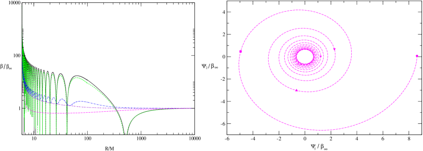
Figure 1: Left panel: The dependence of $\beta$ on the radial coordinate $R$ is shown. Since the problem is a linear one we set hereafter the value of the inclination angle at large radii, $\beta_{\infty}$, equal to unity in all Figs. The parameter $\tilde{\delta}=10^{-2}$. The solid curve is obtained by setting $\alpha=0$ in (62). The short dashed curve represents our analytical results discussed above. We use the expression for $\beta$ given by equation (83) in an intermediate region of $R$, when $R-R_{ms}\ll 1$ the expression (71) is used and when $R\sim R_{2}$ or larger we use equation (79). The dot-dashed, dot-double dashed, long dashed curves correspond to $\alpha=10^{-4}$, $10^{-3}$ and $10^{-2}$, respectively. Right panel: The result of integration of equation (62) presented in parametric form. $\Psi_{1}=Re{\bf W}=\beta\cos\gamma$ and $\Psi_{2}=Im{\bf W}=\beta\sin\gamma$, $\tilde{\delta}=10^{-2}$ and $\alpha=10^{-2}$ for this plot. The circle, square, triangle (pointing up), triangle (pointing down) and the star correspond to $R=6$, $6.1$, $6.2$, $6.3$ and $7$, respectively.

4.3.1 Dependencies of $\beta$ and $\gamma$ on $R$

At first let us discuss the dependency of $\beta$ on $R$ for the case of relatively small viscosity parameter $\alpha\leq 10^{-2}$ and $a>0$. This case is represented in Figs. 1 (left panel) and 2, for $\tilde{\delta}=10^{-2}$ and $0.1$, respectively. As seen from these Figs. the oscillations of the inclination angle are quite prominent for the case when $\alpha=0$ in equation (62) as well as for the case of quite small $\alpha=10^{-4}$. Also, it is seen that our analytic theory described above gives the curve (the left panel in Fig. 1), which is in a quite good agreement with the numerical one calculated for $\alpha=0$. Effects of viscosity tend to smooth out the oscillations, which disappear for the curves with $\alpha=10^{-3}$ and $10^{-2}$ on the left panel in Fig. 1. The similar tendency is seen in Fig. 2 where, additionally, the case of relatively large $\alpha>10^{-2}$ is shown as well. It is clear from these Figs. that when $\alpha$ is small the inclination angle grows with decrease of $R$ either on average or monotonically. Thus, in these cases the disc does not align with the black hole equatorial plane and the Bardeen-Petterson effect is absent. Note that the smooth curves do not have sharp gradients of the inclination angle and, accordingly, they correspond to solutions, where the shear velocities induced in the disc are relatively small. Therefore, these solutions may be physically realistic even for relatively large values of the inclination angle at large radii, $\beta_{\infty}$.

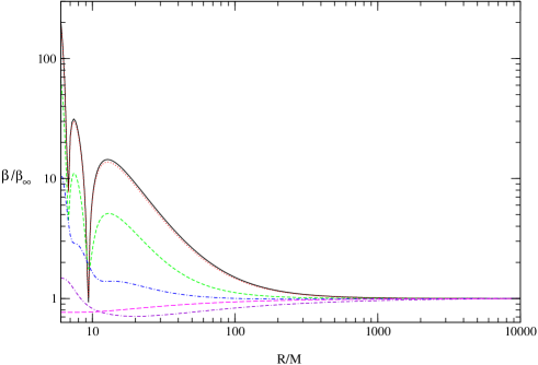
Figure 2: The same as on the left panel in Fig. 1 but for $\tilde{\delta}=10^{-1}$. The solid, dotted, short dashed, dot-dashed, dot-double dashed and long dashed curves correspond to $\alpha=0,10^{-4}$, $10^{-3}$, $10^{-2}$, $10^{-1}$ and $1$, respectively.

Instead of showing dependencies of the second Euler angle $\gamma$ on $R$ we plot curves corresponding to our solutions on the plane $(\Psi_{1}=\beta\cos\gamma,\Psi_{2}=\beta\sin\gamma)$, which depend parametrically on $R$. Since the angle $\gamma$ does not change significantly with $R$ for very small values of $\alpha$ and the corresponding curves are close to straight lines, the case of small viscosity parameters is represented by only one curve corresponding to the solution with $\alpha=10^{-2}$, see the right panel in Fig. 1. One can see from this Fig. that this curve has a form of a tight spiral. In this case $\beta_{0}\sim 8$ and $\gamma=0$, so the curve starts at $R=R_{ms}$ when $\Psi_{1}\sim 8$ and $\Psi_{2}=0$. It spirals clockwise with increase of $R$, i.e. in the direction opposite to the orbital motion and black hole rotation, which are counterclockwise.

The dependence of $\beta$ on $R$ as well as the solutions in the parametric form for $\tilde{\delta}=10^{-2}$ and larger values of $\alpha=0.05$, $0.1$, $0.2$ and $1$ are shown in Fig. 3. From the left panel in Fig. 3 one can see that in this case the inclination angle monotonically decrease in practically the whole range of $R$ while there is a small increase of the angle close to $R_{ms}$. In general, the ratio of $\beta_{0}/\beta_{\infty}$ is quite small and this may be interpreted as manifestation of the Bardeen-Petterson effect. Contrary to the case of the low viscosity discussed above the initial value of $\beta_{0}$ is smaller than one, thus for the curves on the right panel of Fig. 3 $\beta=\sqrt{\Psi_{1}^{2}+\Psi_{2}^{2}}$ increases its value when the curves spiral from $R_{ms}$ to larger $R$. The direction of spiralling with the increase of $R$ is also clockwise similar to what is shown on right panel of Fig. 1.

However, returning to Fig. 2 we see that for $\tilde{\delta}=10^{-1}$ the Bardeen-Petterson effect is absent even when $\alpha\sim 1$ in the sense that the ratio $\beta_{0}/\beta_{\infty}$ remains to be of order of unity.

Thus, in the case of $a>0$ the Bardeen-Petterson effect occurs only when the viscosity parameter $\alpha$ is sufficiently large and $\tilde{\delta}$ is sufficiently small.

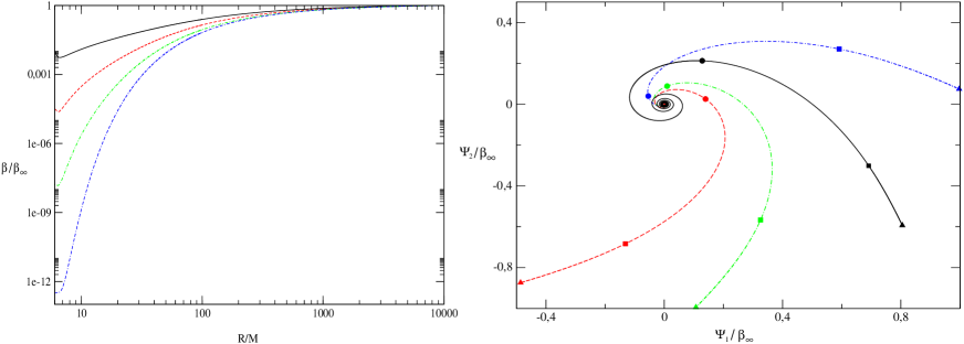
Figure 3: Same as in Fig. 1 but for larger values of $\alpha$. The solid, dashed, dot-dashed and dot-double dashed curves are plotted for $\alpha=0.05$, $0.1$, $0.2$ and $1$, respectively. Curves of the same style correspond to the same $\alpha$ on both panels. Different symbols on the right panel correspond to different values of $R$, $R=100$, $10^{3}$ and $10^{4}$ for the circles, squares and triangles, respectively.

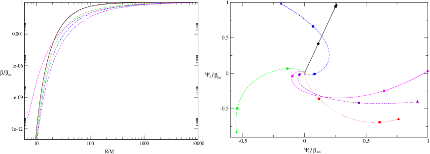
Figure 4: The same as in Fig. 1 but for the case of the black hole rotating in the opposite sense with respect to the disc rotation, $a<0$. The solid, dotted, short-dashed, dot-dashed, dot-double dashed and the long-dashed curves correspond to $\alpha=0$, $0.01$, $0.05$, $0.1$, $0.2$ and $1$, respectively. Curves of the same style correspond to the same $\alpha$ on both panels and positions of different symbols on the right panel correspond to the same $R$ as in Fig. 3.

The case of $a<0$ is shown in Fig. 4, for $\tilde{\delta}=10^{-2}$ and a range of values of $\alpha$. As is seen from this Fig. contrary to the previous case the disc always aligns with the black hole. This is valid even in the case of setting $\alpha=0$ in (62), which is described by the solid curve in Fig. 4. The curves with small values of $\alpha$ are close to this limiting curve. It is interesting to point out that as seen from the right panel in Fig. 4 the direction of spiralling when $R$ runs from smaller to larger radii is opposite to the case of $a>0$. Now the curves spirals in the direction of the orbital motion but, again, opposite to the direction of the black hole rotation. Thus, the direction of spiralling is always opposite to the black hole rotation. This may have some observational consequences.

4.3.2 An analysis of behaviour of the solutions for the case $a>0$ on the parameter plane ($\alpha,\tilde{\delta}$)

As we discuss above our equation contains two independent parameters - $\alpha$ and $\tilde{\delta}$. It is of interest to describe how the most important characteristics of the solutions such as the ratio $\beta_{0}/\beta_{\infty}$ depend on them.

In Fig. 5 we show the dependence of this ratio on $\tilde{\delta}$ for various sufficiently small values of $\alpha$. One can see that the curve corresponding to $\alpha=0$ experiences a quite non-monotonic behaviour with series of peaks at some successive values of $\tilde{\delta}$. Since the analytical curve based on our WKBJ theory developed above is in excellent agreement with the numerical one we can identify these peaks with the resonant solutions of (62) with $\alpha=0$ for which the value of the inclination angle tends to zero when $R\rightarrow\infty$. The positions of these peaks are, accordingly, given by equation (89). Note also that our simple estimate (90) of the dependence of $\beta_{0}/\beta_{\infty}$ on $\tilde{\delta}$ provides a very good approximation to the numerical curve when the resonance peaks are not taken into account.

From the analytical theory it follows that when $\alpha=0$ formally the amplitude of peaks in (5) is infinite. When a small value of $\alpha$ is taken into account the peak’s amplitudes get finite values decreasing with increase of $\alpha$ and/or $\tilde{\delta}$. For a relatively large value of $\alpha=10^{-2}$ the peaks practically disappear and the corresponding curve strongly deviates from the theoretical one. In the case the values of $\beta_{0}/\beta_{\infty}\sim 10$ in the whole range of considered values of $\tilde{\delta}$.

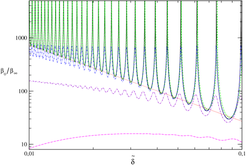
Figure 5: The dependence of the ratio of the inclination angle at the last stable orbit to the inclination angle at a large radius, $\beta_{0}/\beta_{\infty}$, on the parameter $\tilde{\delta}$. The solid curve is calculated for $\alpha$ set to zero in (62), the short dashed curve represents $C_{tot}^{-1}(\tilde{\delta})$, where $C_{tot}$ is defined in equation (88) while the dotted curve represents our simple estimate (90), which does not take into account the effect of the resonances. The dot-dashed, dot-double dashed and the long dashed curves are for $\alpha=10^{-4}$, $10^{-3}$ and $10^{-2}$, respectively.

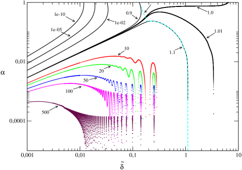
Figure 6: Levels of constant ratios of $\beta_{0}/\beta_{\infty}$ on the plane $(\tilde{\delta}$, $\alpha)$ of the parameters of the problem. Arrows show the values of $\beta_{0}/\beta_{\infty}$ for each curve. The dashed curve on the right hand side of the plot separates a region on the parameter plane, where a change of $\beta$ with $R$ is larger than 10 per cent of $\beta_{\infty}$ (to the left of this curve) from the region, where the black hole influence on the disc twist is relatively small and the change is less than 10 per cent (to the right of the curve).

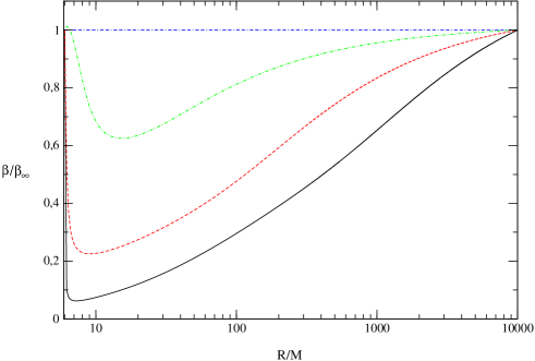
Figure 7: Dependencies of $\beta$ on $R$ along the curve in Fig. 6, where $\beta_{0}/\beta_{\infty}=1$. The values of $\tilde{\delta}$ are equal to $10^{-3}$, $10^{-2}$, $10^{-1}$ and $1$ for the solid, dashed, dot-dashed and dot-double dashed curves, respectively.

In Fig. 6 we show the curves of constant values of the ratio of $\beta_{0}/\beta_{\infty}$ on the plane $(\tilde{\delta}$, $\alpha)$ of the parameters entering equation (62), for the case of $a>0$ and the value of $\tilde{\delta}$ in the range $10^{-3}<\tilde{\delta}<10$. When this ratio is small the disc aligns with the black hole equatorial plane at small radii. One can see that the area of small values of $\beta_{0}/\beta_{\infty}$ is situated at the upper left part of the plot. The opposite case, where $\beta_{0}/\beta_{\infty}>1$ corresponds to a situation when the Bardeen-Petterson effect is absent. For the considered range of $\tilde{\delta}$ the area in the plot, where $\beta_{0}/\beta_{\infty}>1$ is larger than the area corresponding to the small values of this ratio. The curves corresponding to the levels of $\beta_{0}/\beta_{\infty}\geq 10$ exhibit oscillatory behaviour. This effect is most probably determined by the resonant behaviour of $\beta_{0}/\beta_{\infty}$ at small values of $\alpha$ considered above.

The dashed curve on the right hand side of the plot separates the regions on the parameter plane where the quantity $|\beta(R)/\beta_{\infty}-1|$ is smaller/larger than $0.1$, for all values of $R$. The latter condition is satisfied to the left of this curve, where the disc twist induced by the black hole is sufficiently large. Thus, the black hole significantly influences on the disc only when the value of $\tilde{\delta}$ is sufficiently small, $\tilde{\delta}<0.1-1$ depending on value of $\alpha$.

There is a curve in the plot corresponding to the level of $\beta_{0}/\beta_{\infty}=1$. The dependencies of $\beta(R)$ with parameters $\alpha$ and $\tilde{\delta}$ taken along this curve are shown in Fig. 7. As is seen from this Fig. when $\tilde{\delta}$ is sufficiently small the angle $\beta$ behaves in a non-monotonic way, though the curves are smooth and no oscillations of the inclination angle are observed. Such a behaviour looks realistic and it may have serious consequences for the disc structure itself since the inner parts of the disc strongly irradiate the outer part in such cases. Also, it may have some interesting outcomes for spectra modelling, etc.

5 Discussion

In this Paper we derive dynamical equations describing evolution and stationary configurations of a fully relativistic thin twisted disc around a slowly rotating black hole. We assume that the disc inclination angle $\beta\ll 1$, the black hole rotational parameter $a$ is small and that the background flat accretion disc is described by the simplest Novikov-Thorne model with a constant value of the Shakura-Sunyaev parameter $\alpha$. With these assumptions being adopted a characteristic evolution time scale of such a disc is much larger than the dynamical time scale. This helps to simplify our analysis to a great extent. It is shown that the final dynamical equations may be formulated as equations for two dynamical complex variables ${\bf W}$ describing the disc twist and warp and ${\bf B}$, which describes shear velocities induced in such a disc. They may be brought to a form similar to what has been used for description of the classical Newtonian twisted discs, see equations (60) and (61).

Since all our variables are well defined in the black hole space-time, the results of integration of our dynamical equations may be directly applied to the problems connected with observations, e.g. obtaining time-dependant luminosity and spectrum of a twisted accretion disc, its shape as seen from large distances, etc..

We analyse stationary configurations of twisted discs in our model and show that they can be fully described by only two parameters - the viscosity parameter $\alpha$ and by the parameter $\tilde{\delta}=\delta_{*}/\sqrt{|a|}$, where $\delta_{*}$ is a characteristic opening angle of a background flat accretion disc.

We consider in details the case of a very low viscosity twisted disc formally setting $\alpha=0$ in equation (62) describing the stationary configurations and develop an analytic approach to the problem of finding of these configurations for the most interesting case $\tilde{\delta}\ll 1$ and $a>0$, which is in excellent agreement with results of numerical integration of (62). We find that the oscillations of the disc inclination angle found by II in their model of a low viscosity twisted disc far from the black hole can be in a different regime in the relativistic region close to the last stable orbit. Namely, for the background flat disc models having singular profiles with the surface density being formally zero at $R_{ms}$ as in the gas pressure dominated NT models the amplitude of disc oscillations and the radial frequency can grow indefinitely large when $\tilde{\delta}\rightarrow 0$. Additionally, in the formal limit $\alpha=0$ there are ”resonant” solutions occurring at some discrete values of $\tilde{\delta}$, which have a finite value of the disc inclination angle at $R=R_{ms}$ and the disc inclination tending to zero when $R\rightarrow\infty$.

Effects of non-zero viscosity tend to smooth out the relativistic oscillations to an extent more prominent than was obtained in an oversimplified model of II. This may explain the results of Nelson & Papaloizou (2000) who didn’t find prominent oscillations of the disc inclination angle in their SPH simulations of the Bardeen-Petterson effect. When viscosity parameter $\alpha$ gets sufficiently large (say, $\alpha\sim 10^{-3}-10^{-2}$ for $\tilde{\delta}=10^{-2}$) the disc oscillations are not observed. Instead of it there is a growth of the inclination angle towards the last stable orbit, which is opposite to what is expected in the standard picture of the Bardeen-Petterson effect. When $\alpha$ gets even larger (say, $10^{-1}$ for $\tilde{\delta}=10^{-2}$) the inclination angle decreases towards $R_{ms}$ as in the standard picture.

In general, there are three possible qualitatively different shapes of the twisted disc depending on values of the parameters of the problem.

1) When $\alpha$ is very small the disc inclination angle oscillates, with the oscillation amplitude growing dramatically towards $R_{ms}$. When the disc inclination angle at large radii is not very small such a regime is probably unphysical. As we discuss in the text in such a case the shear velocities induced in the disc can easily exceed the speed of sound. This may either make the disc more turbulent thus effectively increasing the value of $\alpha$, which may, in its turn, damp the oscillations. On the other hand this can lead to presence of shocks in the disc close to $R_{ms}$. The energy dissipated in the shocks may make the disc thicker. This opens up a possibility of explaining of the presence of more compatible with observations thick discs close to $R_{ms}$ by such a mechanism.

2) When $\alpha$ is moderately small the oscillations are absent. However, the Bardeen-Petterson effect is absent as well. In such a regime the disc inclination can either monotonically grow towards the last stable orbit or exhibit a non-monotonic behaviour decreasing with decrease of $R$ at large radii and increasing at smaller radii, see Figs. 1 and 7. Since the corresponding curves are quite smooth we do not expect large shear velocities, which are proportional to the gradient of ${\bf W}$. Therefore, such a regime may be physically allowed. This can lead to interesting possibilities of modifying the disc structure by strong irradiation of outer parts of the disc by inner parts, can be very important for modelling of spectra of the discs, etc..

3) Finally, when $\alpha$ is sufficiently large the Bardeen-Petterson effect is observed. The region of the parameter plane, where such effect is possible is shown in Fig. 6, for the considered range $10^{-3}<\tilde{\delta}<10$.

Although we consider the rotational parameter of the black hole as a small parameter of the problem we believe that the outlined picture remains qualitatively correct for moderate values of the rotational parameter as well, say when $a\sim 0.5$.

We discuss possible generalisations of our results. At first one can solve time-dependant equations (60) and (61) to clarify dynamics of the twisted discs in the relativistic regime. This will be done in a separate publication. Secondly, one can try to generalise the results to the case of large values of the rotational parameter, $a\sim 1$. We expect that time-dependent equations will be rather cumbersome since in this case the evolution time scale will be of the order of the dynamical one and many terms neglected in our analysis must be taken into account. The generalisation to the stationary case looks relatively straightforward. However, it may happen that our twisted coordinate system based on the cylindrical coordinate system is less convenient when $a\sim 1$ than a twisted coordinate system based on the spherical coordinates similar to what was introduced by Ogilvie (1999) for the classical Newtonian twisted discs. One may also try to include (at least, at some phenomenological level) the effects of back reaction on the background flat disc model determined by the large shear velocities induced in the twisted disc, and the disc self-irradiation. Additionally, as we discuss in Section 2.4 equations describing the flat disc models used in this paper are invalid very close to the last stable orbit, where the radial drift velocity gets larger than the sound speed, see equation (42). One may try to use a slim disc model close to $R_{ms}$ as a background model for our equations to overcome this difficulty. Finally, one may use the shape of the stationary configurations calculated in this paper to model different observed characteristics of particular sources.

Appendix A The one forms and connection coefficients

A.1 The forms

The transformation law (7) may be considered as a rotation to another Cartesian coordinate system $(\tau=t,x_{1}=r\cos\psi,y_{1}=r\sin\psi,z_{1}=\xi)$ with help of the rotational matrix entering (7). Let us call this matrix as $\bf A$. The one forms (10-13) are related to the forms associated with the new coordinates $(\tau,x_{1},y_{1},z_{1})$ as the forms (6) are related to the forms associated with the old one $(t,x,y,z)$. Explicitly, the transformation between the forms (6) and the forms associated with the coordinates $(t,x,y,z)$ may be written as

$$\mbox{\boldmath$\bar{\omega}$}_{Car}={\bf B}\mbox{\boldmath$\bar{\omega}$}_{c},$$ (95)

where $\bar{\omega}$ are vectors having the corresponding one forms as their components, e.g. $\mbox{\boldmath$\bar{\omega}$}_{c}$ has the components $(\mbox{\boldmath$\omega$}^{(t)},\mbox{\boldmath$\omega$}^{(r)},\mbox{\boldmath$\omega$}^{(\phi)},\mbox{\boldmath$\omega$}^{(z)})$, etc.. $\bf B$ is a rotational matrix with components

$$\begin{array}[]{cccc}\left(\begin{array}[]{cccc}1&0&0&0\\ 0&cos\phi&-\sin\phi&0\\ 0&sin\phi&cos\phi&0\\ 0&0&0&1\end{array}\right)\end{array}.$$ (96)

Analogously, the transformation between the vector containing the forms (10-13), $\mbox{\boldmath$\bar{\omega}$}_{tw}$, and the vector containing the forms corresponding to the new Cartesian system, $\mbox{\boldmath$\bar{\omega}$}_{CarNew}$, may be written as

$$\mbox{\boldmath$\bar{\omega}$}_{CarNew}={\bf C}\mbox{\boldmath$\bar{\omega}$}_{tw},$$ (97)

where the rotational matrix ${\bf C}$ is obtained from ${\bf B}$ by change of the angle: $\phi\rightarrow\psi$. Accordingly, we have

$$\mbox{\boldmath$\bar{\omega}$}_{tw}={\bf C}^{T}{\bf A}{\bf B}\mbox{\boldmath$\bar{\omega}$}_{c}.$$ (98)

The rotational matrix ${\bf C}^{T}{\bf A}{\bf B}$ has the components

$$\begin{array}[]{cccc}\left(\begin{array}[]{cccc}1&0&0&0\\ 0&1&(\xi/r)\beta\cos\psi&\beta\sin\psi\\ 0&-(\xi/r)\beta\cos\psi&1&\beta\cos\psi\\ 0&-\beta\sin\psi&-\beta\cos\psi&1\\ \end{array}\right)\end{array}.$$ (99)

Since the transformation (98) is given by an orthogonal matrix the transformation between the corresponding sets of adjoint basis vectors is the same.

A.2 The connection coefficients

The non-trivial connection coefficients are given by the following expressions:

$$\begin{array}[]{ll}\Gamma_{\tau r\tau}=\frac{K_{1}^{\prime}}{K_{1}K_{2}},&\Gamma_{\tau r\varphi}=a\frac{K_{3}}{K_{2}^{2}}\,\left(1-\frac{1}{2}\left(r-\xi Z\right)K_{4}\right),\\ &\\ \Gamma_{\tau r\xi}=-a\frac{K_{3}}{K_{2}^{2}}\partial_{\varphi}Z\left(1-\frac{1}{2r}\left(r^{2}+\xi^{2}\right)K_{4}\right),&\Gamma_{\tau\varphi r}=-\Gamma_{\tau r\varphi},\\ &\\ \Gamma_{\tau\varphi\xi}=a\frac{K_{3}}{K_{2}^{2}}\left(Z+\frac{\xi}{2r}\left(r-\xi Z\right)K_{4}\right),&\Gamma_{\tau\xi\tau}=\frac{\xi}{r}\frac{K_{1}^{\prime}}{K_{1}K_{2}},\\ &\\ \Gamma_{\tau\xi r}=-\Gamma_{\tau r\xi},&\Gamma_{\tau\xi\varphi}=-\Gamma_{\tau\varphi\xi},\\ &\\ \Gamma_{r\varphi\tau}=\frac{\xi}{r}\frac{1}{K_{1}}\partial_{\varphi}U-\Gamma_{\tau r\varphi},&\Gamma_{r\varphi r}=\frac{\xi}{r}\frac{1}{K_{2}}\partial_{\varphi}W,\\ &\\ \Gamma_{r\varphi\varphi}=\frac{(rK_{2})^{\prime}}{rK_{2}^{2}}-a\xi\frac{K_{3}}{K_{1}K_{2}}\partial_{\varphi}U,&\Gamma_{r\xi\tau}=\frac{U}{K_{1}}-\Gamma_{\tau r\xi},\\ &\\ \Gamma_{r\xi r}=\frac{W}{K_{2}}-\frac{\xi}{r}\frac{K_{2}^{\prime}}{K_{2}^{2}},&\Gamma_{r\xi\varphi}=-ar\frac{K_{3}}{K_{1}K_{2}}U,\\ &\\ \Gamma_{r\xi\xi}=\frac{K_{2}^{\prime}}{K_{2}^{2}},&\Gamma_{\varphi\xi\tau}=\frac{1}{K_{1}}\partial_{\varphi}U-\Gamma_{\tau\varphi\xi},\\ &\\ \Gamma_{\varphi\xi r}=\frac{1}{K_{2}}\partial_{\varphi}W,&\Gamma_{\varphi\xi\varphi}=-\frac{\xi}{r}\frac{K_{2}^{\prime}}{K_{2}^{2}}-ar\frac{K_{3}}{K_{1}K_{2}}\partial_{\varphi}U,\\ &\\ \\ \end{array}$$ (100)

where $K_{4}\equiv(K_{3}/K_{1})(K_{1}/K_{3})^{\prime}$.
Other non-zero connection coefficients are obtained with help of antisymmetry over the first two indices: $\Gamma_{abc}=-\Gamma_{bac}$.

Appendix B Perturbed equations of motion

As we discuss in Section 3 our subset of equations describing the disc twist follows from equations (20) after the procedure outlined in this Section.

The $\tau$-component of (20) gives

$$K\frac{K_{2}}{K_{1}}(U^{\tau})^{2}\dot{\rho}_{1}+\left(2U^{\varphi}-ar\frac{K_{3}}{K_{2}}\frac{(U^{\varphi})^{2}+(U^{\tau})^{2}}{U^{\tau}}\right)\frac{K_{2}}{K_{1}}\rho\dot{v}^{\varphi}+\frac{1}{r}U^{\tau}U^{\varphi}\partial_{\varphi}\rho_{1}+\frac{1}{r}\frac{(U^{\varphi})^{2}+(U^{\tau})^{2}}{U^{\tau}}\rho\partial_{\varphi}v^{\varphi}+\\ \partial_{r}(\rho U^{\tau}v^{r})+\partial_{\xi}\rho U^{\tau}v^{\xi}+\frac{(rK_{1}^{2}K_{2}^{2})^{\prime}}{rK_{1}^{2}K_{2}^{2}}\rho U^{\tau}v^{r}+F_{\nu}^{\tau}=r\partial_{\xi}\rho(U^{\tau})^{2}K\frac{K_{2}}{K_{1}}U+\frac{\xi}{r}\rho U^{\tau}U^{\varphi}\partial_{\varphi}W,$$ (101)

where

$$K=\left(1-ar\frac{K_{3}}{K_{2}}\frac{U^{\varphi}}{U^{\tau}}\right),$$

and the $r$, $\varphi$ and $\xi$-components give, respectively,

$$K\frac{K_{2}}{K_{1}}U^{\tau}\dot{v}^{r}+\frac{U^{\varphi}}{r}\partial_{\varphi}v^{r}-\left[2\frac{K_{1}^{\prime}}{K_{1}U^{\varphi}}+a\frac{K_{1}}{rK_{2}U^{\tau}}\left(\frac{r^{2}K_{3}}{K_{1}}\right)^{\prime}\right]v^{\varphi}+{1\over\rho}F^{r}_{\nu}=\\ Wr\frac{\partial_{\xi}p}{\rho}-a\xi\frac{K_{3}^{2}}{K_{1}K_{2}}\left(\frac{K_{1}}{K_{3}}\right)^{\prime}ZU^{\tau}U^{\varphi},$$ (102)

$$K\frac{K_{2}}{K_{1}}U^{\tau}U^{\varphi}\dot{\rho}_{1}+\left(\frac{(U^{\varphi})^{2}+(U^{\tau})^{2}}{U^{\tau}}-2ar\frac{K_{3}}{K_{2}}U^{\varphi}\right)\frac{K_{2}}{K_{1}}\rho\dot{v}^{\varphi}+\frac{(U^{\varphi})^{2}}{r}\partial_{\varphi}\rho_{1}+2\frac{U^{\varphi}}{r}\rho\partial_{\varphi}v^{\varphi}+\\ \partial_{r}(\rho U^{\varphi}v^{r})+\partial_{\xi}\rho U^{\varphi}v^{\xi}+\frac{(r^{2}K_{1}K_{2}^{3})^{\prime}}{r^{2}K_{1}K_{2}^{3}}U^{\varphi}\rho v^{r}-a\frac{K_{1}}{rK_{2}}\left(\frac{r^{2}K_{3}}{K_{1}}\right)^{\prime}U^{\tau}\rho v^{r}+F^{\varphi}_{\nu}=\\ K\frac{K_{2}}{K_{1}}r\partial_{\xi}\rho U^{\tau}U^{\varphi}U+\frac{\xi}{r}\rho(U^{\varphi})^{2}\partial_{\varphi}W,$$ (103)

and

$$K\frac{K_{2}}{K_{1}}ru^{\tau}\dot{v}^{\xi}+U^{\varphi}\partial_{\varphi}v^{\xi}+r\frac{\partial_{\xi}p_{1}}{\rho}+\xi\frac{(U^{\varphi})^{2}}{r}\left(1-2ar\frac{K_{3}}{K_{2}}\frac{U^{\tau}}{U^{\varphi}}\right)\frac{\rho_{1}}{\rho}+\\ 2\xi U^{\varphi}v^{\varphi}\left[\frac{K_{1}^{\prime}}{K_{1}}-\frac{K_{2}^{\prime}}{K_{2}}-\frac{ar}{2}\frac{K_{3}^{2}}{K_{1}K_{2}}\left(\frac{K_{1}}{K_{3}}\right)^{\prime}\left(\frac{U^{\tau}}{U^{\varphi}}+\frac{U^{\varphi}}{U^{\tau}}\right)\right]+{r\over\rho}F^{\xi}_{\nu}=\\ -\left[\frac{K_{2}}{K_{1}}\partial_{\varphi}U-2a\frac{K_{3}Z}{K_{2}}+a\frac{\xi^{2}}{r}\frac{K_{3}^{2}Z}{K_{1}K_{2}}\left(\frac{K_{1}}{K_{3}}\right)^{\prime}\right]rU^{\tau}U^{\varphi}+ar^{2}\frac{K_{3}}{K_{1}}(U^{\varphi})^{2}\partial_{\varphi}U.$$ (104)

where $F_{\nu}^{i}$ are determined by the presence of viscous interactions in the disc. Since these interactions lead to a non-zero value of the drift component, $U^{r}$, we include terms containing $U^{r}$ in $F_{\nu}^{i}$ excepting the terms proportional to $U^{r}$ through the dependence of $v^{\xi}$ on $U^{r}$, see equation (44) to keep the notation uniform.

Explicitly, we have from (20)

$$F^{\tau}_{\nu}={U^{\varphi}\over U^{\tau}}(\partial_{\xi}T_{\nu}^{\varphi\xi}-rW\partial_{\xi}T_{\nu}^{r\varphi})-r\partial_{\xi}\rho U^{\tau}U^{r}W,\\ F^{\varphi}_{\nu}=(\partial_{\xi}T_{\nu}^{\varphi\xi}-rW\partial_{\xi}T_{\nu}^{r\varphi})-r\partial_{\xi}\rho U^{\varphi}U^{r}W,\quad F_{\nu}^{r}=\partial_{\xi}T_{\nu}^{r\xi},$$ (105)

and

$$F^{\xi}_{\nu}={1\over rK_{1}K_{2}^{3}}\partial_{r}(rK_{1}K_{2}^{3}T_{\nu}^{r\xi})+\partial_{\xi}T_{\nu}^{\xi\xi}+{1\over r}\partial_{\varphi}T_{\nu}^{\varphi\xi}+\\ \partial_{\varphi}W(T_{\nu}^{r\varphi}+T^{r\varphi}_{adv})+a\frac{K_{1}}{rK_{2}}\left(\frac{r^{2}K_{3}}{K_{1}}\right)^{{}^{\prime}}\partial_{\varphi}Z\left(\frac{U^{\varphi}}{U^{\tau}}T_{\nu}^{r\varphi}+\frac{U^{\tau}}{U^{\varphi}}T^{r\varphi}_{adv}\right),$$ (106)

where $T^{r\varphi}_{adv}=\rho U^{\varphi}U^{r}$. $T_{\nu}^{ij}$ are components of the viscous stress tensor given by equations (21) and (22) relevant for our purposes:

$$T_{\nu}^{r\xi}=-{\eta\over K_{2}}(\partial_{\xi}v^{r}+U^{\varphi}\partial_{\varphi}W),\\ T_{\nu}^{\varphi\xi}=-{\eta\over K_{2}}\left(\partial_{\xi}v^{\varphi}-2a{K_{3}\over K_{2}}U^{\tau}(U^{\varphi})^{2}Z\right),\quad T_{\nu}^{r\varphi}=-\eta r\left({U^{\varphi}\over rK_{2}}\right)^{\prime},$$ (107)

where we use equations (21) and (22).

Note that we take into account all explicit terms of zero and first order in $a$ in equations (101-107). As we discuss in the main text, in fact, the only term linear in $a$, which is important for our purposes, is the gravitomagnetic term - the second term in the square brackets on the right hand side of (104), see equation (112) below. Other terms may be important in other studies and are shown for a reference. The background quantities $U^{\tau}$, $U^{\varphi}$ and $\partial_{\xi}p/\rho$ can also be easily developed up to the linear in $a$ order, and, for completeness, we show them below. We have

$$U^{\varphi}=U_{S}^{\varphi}-a\,\frac{(U_{S}^{\varphi})^{2}U_{S}^{\tau}}{R^{1/2}(R-2)^{1/2}},\quad U^{\tau}=U_{S}^{\tau}-a\,\frac{(U_{S}^{\varphi})^{3}}{R^{1/2}(R-2)^{1/2}},$$ (108)

where $U_{S}^{\varphi}$ and $U^{\tau}_{S}$ are given by (25), and

$$\frac{\partial_{\xi}p}{\rho}=-\frac{(U_{S}^{\varphi})^{2}}{r^{2}}\xi\left[1-6a\frac{K_{1}}{rK_{2}}U_{S}^{\tau}U_{S}^{\varphi}\right]=\frac{(U^{\varphi})^{2}}{r^{2}}\frac{\Omega_{\perp}^{2}}{\Omega^{2}}\xi,$$ (109)

where

$$\Omega_{\perp}=\Omega-\Omega_{LT},$$ (110)

we remind that $\Omega=R^{-3/2}$ and the frequency of the Lense-Thirring precession (see e.g. Aliev $\&$ Galtsov 1981, Kato 1990), $\Omega_{LT}$, is given by the expression

$$\Omega_{LT}=a\frac{K_{1}K_{3}}{K_{2}^{2}}=2aR^{-3}$$ (111)

It is important to note that from equation (104) it follows that this characteristic frequency determines the disc’s evolution in a certain regime. In order to show it let us temporarily assume that we consider a pressureless, inviscid disc with gas particles moving on circular orbits around a black hole. In this case we can set $p_{1}=\rho_{1}=v^{\varphi}=0$ in (104). The last two terms on the right hand side can be also neglected since they contain products of two small parameters: $a(h/r)^{2}$ and $a(t_{d}/t_{tw})$, respectively. Accordingly, we obtain from (104)

$$\partial_{\varphi}U=\Omega_{LT}Z.$$ (112)

Remembering that $U=\dot{Z}$ we see that in this case the disc rings precess with the precession frequency equal to $\Omega_{LT}$.

Appendix C The law of conservation of angular momentum

The space-time of a Schwarzschild black hole is symmetric with respect to transformations belonging to the three-dimensional group of rotations, $O(3)$. Accordingly, equations of motion contain three conserved quantities, which may be identified with three components of angular momentum. Conservation of the components perpendicular to the axis $z$ requires a special divergent form of equation (48) (or (61)). In order to see that this equation has, indeed, such a form let us represent the term on the right hand side as $-{1\over r^{2}K_{2}^{4}}{\partial\over\partial r}F$ and the quantity $F$ as $F=C_{1}\cos\varphi+C_{2}\sin\varphi$, where $C_{1}$ and $C_{2}$ are functions of $r$ and $\tau$. Introducing the complex notation used above we rewrite (48) as

$$\Sigma U^{\tau}U^{\varphi}(\dot{\bf W}-i\Omega_{LT}{\bf W})+{K_{1}\over K_{2}}(\Sigma U^{\varphi}U^{r}+\bar{T}_{\nu}^{r\varphi}){\bf W}^{\prime}=-{1\over r^{2}K_{2}^{4}}{\partial\over\partial r}{\bf F},$$ (113)

where ${\bf F}=C_{1}+iC_{2}$. We multiply (113) by $r^{2}K^{2}$ and integrate over $r$ from some radius $r_{in}$ to $r_{out}>r_{in}$. We get

$$\dot{\bf L}-i{\bf T}+{\bf I}={\bf F}(r_{in})-{\bf F}(r_{out}),$$ (114)

where

$${\bf L}=\int^{r_{out}}_{r_{in}}drr^{2}K_{2}^{4}\Sigma U^{\tau}U^{\varphi}{\bf W},\quad{\bf T}=\int^{r_{out}}_{r_{in}}drr^{2}K_{2}^{4}\Sigma U^{\tau}U^{\varphi}\Omega_{LT}{\bf W},$$ (115)

and

$${\bf I}=\int^{r_{out}}_{r_{in}}drr^{2}K_{1}K_{2}^{3}(\Sigma U^{\varphi}U^{r}+\bar{T}_{\nu}^{r\varphi}){\bf W}^{\prime}.$$ (116)

It can be shown that $\bf L$ is proportional to a linear combination of $x$ and $y$-components of the disc angular momentum within the region $r_{in}<r<r_{out}$, and $\bf T$ is the corresponding torque term provided by the gravitomagnetic force.

The term ${\bf I}$ can be transformed with help of equation reflecting the law of conservation of angular momentum for a background disc model

$${1\over r^{2}K_{1}K_{2}^{3}}{d\over dr}(r^{2}K_{1}K_{2}^{3}(\Sigma U^{\varphi}U^{r}+\bar{T}_{\nu}^{r\varphi}))+2qU^{\varphi}=0,$$ (117)

where $q$ is flux of radiation from the disc surface . We integrate (116) by parts and use (117) to get

$$\dot{\bf L}-i{\bf T}+2\int^{r_{out}}_{r_{in}}drr^{2}K_{1}K_{2}^{3}qU^{\varphi}{\bf W}={\bf F}(r_{in})-{\bf F}(r_{out})+{\bf I}(r_{in})-{\bf I}(r_{out}).$$ (118)

Equation (118) shows that when the black hole is not rotating (${\bf T}=0$) a change of the angular momentum content within a region of the disc is determined by fluxes of angular momentum through the region inner and outer boundaries and angular momentum flux carried by radiation emitted from the disc surface. Thus, equation (48) has the required divergent form.

References

- Aliev & Galtsov (1981) Aliev A. N., Galtsov D. V., 1981, General Relativity and Gravitation, 13, 899
- Bachev (1999) Bachev R., 1999, A&A, 348, 71
- Bardeen & Petterson (1975) Bardeen J. M., Petterson J. A., 1975, ApJ, 195, L65
- Cadez et al. (2003) Cadez A., Brajnik M., Gomboc A., Calvani M., Fanton C., 2003, A&A, 403, 29
- Caproni, Mosquera Cuesta & Abraham (2004) Caproni A., Mosquera Cuesta H. J., Abraham Z., 2004, ApJ, 616, L99
- Caproni et al. (2007) Caproni A., Abraham Z., Livio M., Mosquera Cuesta H. J., 2007, MNRAS, 379, 135
- Demianski & Ivanov (1997) Demianski M., Ivanov P.B., 1997, A&A, 324, 829
- Dexter & Fragile (2011) Dexter J., Fragile, P. C., 2011, ApJ, in press, arXiv:1101.3783
- Ferreira & Ogilvie (2008) Ferreira B. T., Ogilvie G. I., 2008, MNRAS, 386, 2297
- Ferreira & Ogilvie (2009) Ferreira B. T., Ogilvie G. I., 2009, MNRAS, 392, 428
- Fragile & Blaes (2008) Fragile, P. C., Blaes, O. M., 2008, ApJ, 687, 757
- Hatchett, Begelman & Sarazin (1981) Hatchett S.P., Begelman M.C., Sarazin C.L., ApJ, 247, 677