Cloning of a quantum measurement

Abstract

We analyze quantum algorithms for cloning of a quantum measurement. Our aim is to mimic two uses of a device performing an unknown von Neumann measurement with a single use of the device. When the unknown device has to be used before the bipartite state to be measured is available we talk about $1\rightarrow 2$ learning of the measurement, otherwise the task is called $1\rightarrow 2$ cloning of a measurement. We perform the optimization for both learning and cloning for arbitrary dimension of the Hilbert space. For $1\rightarrow 2$ cloning we also propose a simple quantum network that realizes the optimal strategy.

I Introduction

Arbitrary processing of a classical information can be described by strings of bits, and can be performed by a fixed device for example a processor of any personal computer. As a consequence, we do not need to build new devices for different computations, but we just need to copy bit strings carrying the appropriate program. Situation dramatically changes, when the systems carrying the information are governed by quantum mechanics. Unknown states of quantum systems can not be copied perfectly wootzu and the no-programming theorem noprog prevents existence of universal quantum processors. This means that quantum programs can not be copied and that by using registers of qubits (two level quantum systems) one can not deterministically realize all quantum information processing functions with a fixed processor. So in contrast to classical devices, quantum ones cannot be replicated by just copying the program for them. Copying of quantum states was extensively investigated buzek1 ; werner1 ; cavesbroad1 ; superbroad1 ; scarani1 . On the other hand copying of quantum devices did not receive so much attention even though it is a fundamental and equally important quantum information processing task. Similarly to states, quantum transformations are often used in quantum key distribution schemes clonunit ; pirandola1 ; bostrom1 ; lucamarini1 to encode bits, so analysis of possible attacks by cloning them are needed. Cloning of transformations was yet analyzed only for the case of unitary transformations clonunit . In the present paper we investigate cloning of measurement devices, which can be seen as a cloning of certain measure-and-prepare transformations. More precisely, when a measurement is an intermediate step of a quantum procedure its outcome can influence the following operations. This feed forward of the classical outcome can be conveniently described using a quantum system into which the outcome is encoded into perfectly distinguishable orthogonal states. In this sense a quantum measurement with only classical outcomes can be seen as a channel, which first measures the input system and based on the outcome prepares a state from a fixed orthogonal set.

The term cloning of observables has been used in Ref. paris1 referring to state cloning machines preserving the statistics of a class of observables. In the present paper the objective is to actually mimic two uses of an unknown measurement device, while using it only once. We would like to construct a replication strategy that would work for arbitrary von Neumann measurement $\boldsymbol{E}$, even if it is provided as an unknown black box. The most natural operation of a replication strategy is based on modifying the bipartite state before $\boldsymbol{E}$ is actually used. In this case we talk about $1\rightarrow 2$ cloning of a measurement device. The most general representation of any cloning strategy is depicted below

$$\begin{aligned} \lx@xy@svg{\hbox{\raise 0.0pt\hbox{\kern 0.0pt\hbox{\ignorespaces\ignorespaces\ignorespaces\hbox{\vtop{\kern 0.0pt\offinterlineskip\halign{\entry@#!@&&\entry@@#!@\cr&&&&&&&\\&&&&&&&\crcr}}}\ignorespaces{\hbox{\kern 0.0pt\raise 0.0pt\hbox{\hbox{\kern-3.0pt\raise 0.0pt\hbox{\hbox{\kern 3.0pt\raise 0.0pt\hbox{$\textstyle{}$}}}}}}}{\hbox{\kern 10.00002pt\raise 0.0pt\hbox{\hbox{\kern-3.75pt\raise 5.0pt\hbox{$\textstyle{A}$}}}}}{\hbox{\kern 20.00003pt\raise 0.0pt\hbox{\hbox{\kern 5.0pt\raise 0.0pt\hbox{$\textstyle{\hphantom{\;\;\;}}$}}}}}\ignorespaces\ignorespaces\ignorespaces\ignorespaces{}{\hbox{\lx@xy@droprule}}\ignorespaces{}{\hbox{\lx@xy@droprule}}{\hbox{\lx@xy@droprule}}\ignorespaces\ignorespaces{\hbox{\kern 25.00003pt\raise-12.19789pt\hbox{\hbox{\kern 0.0pt\raise 0.0pt\hbox{$\textstyle{\;\;\;}$}}}}}\ignorespaces\ignorespaces\ignorespaces\ignorespaces\ignorespaces{\hbox{\lx@xy@droprule}}\ignorespaces\ignorespaces\ignorespaces\ignorespaces\ignorespaces{\hbox{\lx@xy@droprule}}\ignorespaces\ignorespaces\ignorespaces\ignorespaces\ignorespaces{\hbox{\lx@xy@droprule}}\ignorespaces\ignorespaces\ignorespaces\ignorespaces\ignorespaces{\hbox{\lx@xy@droprule}}{\hbox{\kern 48.33318pt\raise 0.0pt\hbox{\hbox{\kern-3.93124pt\raise 5.0pt\hbox{$\textstyle{C}$}}}}}\ignorespaces\ignorespaces\ignorespaces\ignorespaces{}{\hbox{\lx@xy@droprule}}\ignorespaces{}{\hbox{\lx@xy@droprule}}{\hbox{\lx@xy@droprule}}{\hbox{\kern 58.33319pt\raise 0.0pt\hbox{\hbox{\kern 0.0pt\raise 0.0pt\hbox{$\textstyle{\lx@xy@svgnested{\hbox{\raise 0.0pt\hbox{\kern 12.95831pt\hbox{{\hbox{\kern-6.47916pt\raise 0.0pt\hbox{\hbox{\kern 2.5pt\raise-3.41666pt\hbox{$\textstyle{\vphantom{\rule{0.0pt}{1.00006pt}\boldsymbol{E}}}$}}}}}{\hbox{\kern-6.47916pt\raise 0.0pt\hbox{\hbox{\kern 0.0pt\raise 0.0pt\hbox{\cirbuild@}}}}}\ignorespaces{\hbox{\kern-7.95831pt\raise 0.0pt\hbox{\hbox{\kern 0.0pt\raise-3.41666pt\hbox{$\textstyle{\boldsymbol{E}}$}}}}}\ignorespaces\ignorespaces\ignorespaces\ignorespaces\ignorespaces{\hbox{\kern-12.95831pt\raise 6.47916pt\hbox{\hbox{\kern 0.0pt\raise-3.41666pt\hbox{$\textstyle{\hphantom{\boldsymbol{E}}}$}}}}}\ignorespaces\ignorespaces\ignorespaces{\hbox{\lx@xy@droprule}}\ignorespaces\ignorespaces\ignorespaces\ignorespaces\ignorespaces{\hbox{\kern-12.95831pt\raise-6.47916pt\hbox{\hbox{\kern 0.0pt\raise-3.41666pt\hbox{$\textstyle{\hphantom{\boldsymbol{E}}}$}}}}}\ignorespaces\ignorespaces\ignorespaces{\hbox{\lx@xy@droprule}}\ignorespaces\ignorespaces\ignorespaces{\hbox{\kern-12.95831pt\raise 6.47916pt\hbox{\hbox{\kern 0.0pt\raise-3.41666pt\hbox{$\textstyle{\hphantom{\boldsymbol{E}}}$}}}}}\ignorespaces\ignorespaces\ignorespaces{\hbox{\kern-12.95831pt\raise-6.47916pt\hbox{\hbox{\kern 0.0pt\raise-3.41666pt\hbox{$\textstyle{\hphantom{\boldsymbol{E}}}$}}}}}\ignorespaces\ignorespaces\ignorespaces{\hbox{\lx@xy@droprule}}}}}}}$}}}}}\ignorespaces\ignorespaces\ignorespaces\ignorespaces{}{\hbox{\lx@xy@droprule}}\ignorespaces{}{\hbox{\lx@xy@droprule}}{\hbox{\lx@xy@droprule}}{\hbox{\kern 87.77068pt\raise 0.0pt\hbox{\hbox{\kern-4.27847pt\raise 5.0pt\hbox{$\textstyle{D}$}}}}}\ignorespaces\ignorespaces\ignorespaces\ignorespaces{}{\hbox{\hbox{\kern 0.0pt\raise-1.0pt\hbox{\lx@xy@droprule}}\hbox{\kern 0.0pt\raise 1.0pt\hbox{\lx@xy@droprule}}}}\ignorespaces{}{\hbox{\hbox{\kern 0.0pt\raise-1.0pt\hbox{\lx@xy@droprule}}\hbox{\kern 0.0pt\raise 1.0pt\hbox{\lx@xy@droprule}}}}{\hbox{\hbox{\kern 0.0pt\raise-1.0pt\hbox{\lx@xy@droprule}}\hbox{\kern 0.0pt\raise 1.0pt\hbox{\lx@xy@droprule}}}}{\hbox{\kern 97.77069pt\raise 0.0pt\hbox{\hbox{\kern 5.0pt\raise 0.0pt\hbox{$\textstyle{\hphantom{\;\;\;}}$}}}}}\ignorespaces\ignorespaces\ignorespaces\ignorespaces{}{\hbox{\hbox{\kern 0.0pt\raise-1.0pt\hbox{\lx@xy@droprule}}\hbox{\kern 0.0pt\raise 1.0pt\hbox{\lx@xy@droprule}}}}\ignorespaces{}{\hbox{\hbox{\kern 0.0pt\raise-1.0pt\hbox{\lx@xy@droprule}}\hbox{\kern 0.0pt\raise 1.0pt\hbox{\lx@xy@droprule}}}}{\hbox{\hbox{\kern 0.0pt\raise-1.0pt\hbox{\lx@xy@droprule}}\hbox{\kern 0.0pt\raise 1.0pt\hbox{\lx@xy@droprule}}}}{\hbox{\kern 126.10384pt\raise 0.0pt\hbox{\hbox{\kern-3.0pt\raise 0.0pt\hbox{\hbox{\kern 3.0pt\raise 0.0pt\hbox{$\textstyle{}$}}}}}}}{\hbox{\kern 0.0pt\raise-24.3958pt\hbox{\hbox{\kern-3.0pt\raise 0.0pt\hbox{\hbox{\kern 3.0pt\raise 0.0pt\hbox{$\textstyle{}$}}}}}}}{\hbox{\kern 10.00002pt\raise-24.3958pt\hbox{\hbox{\kern-4.0434pt\raise 5.0pt\hbox{$\textstyle{B}$}}}}}{\hbox{\kern 20.00003pt\raise-24.3958pt\hbox{\hbox{\kern 5.0pt\raise 0.0pt\hbox{$\textstyle{\hphantom{\;\;\;}}$}}}}}\ignorespaces\ignorespaces\ignorespaces\ignorespaces{}{\hbox{\lx@xy@droprule}}\ignorespaces{}{\hbox{\lx@xy@droprule}}{\hbox{\lx@xy@droprule}}{\hbox{\kern 48.33318pt\raise-24.3958pt\hbox{\hbox{\kern-3.0pt\raise 0.0pt\hbox{\hbox{\kern 3.0pt\raise 0.0pt\hbox{$\textstyle{\ignorespaces\ignorespaces\ignorespaces\ignorespaces}$}}}}}}}\ignorespaces\ignorespaces\ignorespaces\ignorespaces{}{\hbox{\lx@xy@droprule}}\ignorespaces{}{\hbox{\lx@xy@droprule}}{\hbox{\lx@xy@droprule}}{\hbox{\kern 68.05193pt\raise-24.3958pt\hbox{\hbox{\kern-3.0pt\raise 0.0pt\hbox{\hbox{\kern 3.0pt\raise 0.0pt\hbox{$\textstyle{\ignorespaces\ignorespaces\ignorespaces\ignorespaces}$}}}}}}}\ignorespaces\ignorespaces\ignorespaces\ignorespaces{}{\hbox{\lx@xy@droprule}}\ignorespaces{}{\hbox{\lx@xy@droprule}}{\hbox{\lx@xy@droprule}}{\hbox{\kern 87.77068pt\raise-24.3958pt\hbox{\hbox{\kern-3.0pt\raise 0.0pt\hbox{\hbox{\kern 3.0pt\raise 0.0pt\hbox{$\textstyle{\ignorespaces\ignorespaces\ignorespaces\ignorespaces}$}}}}}}}\ignorespaces\ignorespaces\ignorespaces\ignorespaces{}{\hbox{\lx@xy@droprule}}\ignorespaces{}{\hbox{\lx@xy@droprule}}{\hbox{\lx@xy@droprule}}{\hbox{\kern 97.77069pt\raise-24.3958pt\hbox{\hbox{\kern 5.0pt\raise 0.0pt\hbox{$\textstyle{\hphantom{\;\;\;}}$}}}}}\ignorespaces\ignorespaces\ignorespaces\ignorespaces{\hbox{\kern 102.77069pt\raise-12.1979pt\hbox{\hbox{\kern 0.0pt\raise 0.0pt\hbox{$\textstyle{\;\;\;}$}}}}}\ignorespaces\ignorespaces\ignorespaces\ignorespaces\ignorespaces\ignorespaces{\hbox{\lx@xy@droprule}}\ignorespaces\ignorespaces\ignorespaces\ignorespaces\ignorespaces{\hbox{\lx@xy@droprule}}\ignorespaces\ignorespaces\ignorespaces\ignorespaces\ignorespaces\ignorespaces{\hbox{\lx@xy@droprule}}\ignorespaces\ignorespaces\ignorespaces\ignorespaces\ignorespaces\ignorespaces\ignorespaces{\hbox{\lx@xy@droprule}}\ignorespaces{\hbox{\kern 98.10396pt\raise 4.49997pt\hbox{\hbox{\kern 0.0pt\raise-8.99994pt\hbox{$\textstyle{\hbox{\cirbuild@}}$}}}}}\ignorespaces{\hbox{\kern 98.10396pt\raise-28.89577pt\hbox{\hbox{\kern 0.0pt\raise 8.99994pt\hbox{$\textstyle{\hbox{\cirbuild@}}$}}}}}\ignorespaces\ignorespaces\ignorespaces\ignorespaces{}{\hbox{\lx@xy@droprule}}\ignorespaces{}{\hbox{\lx@xy@droprule}}{\hbox{\lx@xy@droprule}}{\hbox{\kern 126.10384pt\raise-24.3958pt\hbox{\hbox{\kern-3.0pt\raise 0.0pt\hbox{\hbox{\kern 3.0pt\raise 0.0pt\hbox{$\textstyle{}$}}}}}}}\ignorespaces}}}}\ignorespaces\end{aligned} \textstyle{A} \textstyle{C} \textstyle{\boldsymbol{E}} \textstyle{D} \textstyle{B} \textstyle{A} \textstyle{C} \textstyle{\boldsymbol{E}} \textstyle{D} \textstyle{B}$$ (1)

(the double wire carries the classical outcome of the measurement).

On the other hand, one might ask how well the task can be accomplished when we use the measurement, before we have an access to the bipartite state of interest. We denote this scenario as $1\rightarrow 2$ learning, and any learning strategy can be depicted as follows

$$\begin{aligned} \lx@xy@svg{\hbox{\raise 0.0pt\hbox{\kern 9.16656pt\hbox{\ignorespaces\ignorespaces\ignorespaces\hbox{\vtop{\kern 0.0pt\offinterlineskip\halign{\entry@#!@&&\entry@@#!@\cr&&&&\\&&&&\\&&&&\\&&&&\\}}}\ignorespaces{\hbox{\kern 0.0pt\raise 0.0pt\hbox{\hbox{\kern-3.0pt\raise 0.0pt\hbox{\hbox{\kern 3.0pt\raise 0.0pt\hbox{$\textstyle{}$}}}}}}}{\hbox{\kern 16.16653pt\raise 0.0pt\hbox{\hbox{\kern-3.0pt\raise 0.0pt\hbox{\hbox{\kern 3.0pt\raise 0.0pt\hbox{$\textstyle{}$}}}}}}}{\hbox{\kern 32.88524pt\raise 0.0pt\hbox{\hbox{\kern-3.0pt\raise 0.0pt\hbox{\hbox{\kern 3.0pt\raise 0.0pt\hbox{$\textstyle{}$}}}}}}}{\hbox{\kern 49.60394pt\raise 0.0pt\hbox{\hbox{\kern-3.75pt\raise 5.0pt\hbox{$\textstyle{A}$}}}}}{\hbox{\kern 56.60391pt\raise 0.0pt\hbox{\hbox{\kern 5.0pt\raise 0.0pt\hbox{$\textstyle{\hphantom{\;\;\;}}$}}}}}\ignorespaces\ignorespaces\ignorespaces\ignorespaces{}{\hbox{\lx@xy@droprule}}\ignorespaces{}{\hbox{\lx@xy@droprule}}{\hbox{\lx@xy@droprule}}{\hbox{\kern 0.0pt\raise-18.99995pt\hbox{\hbox{\kern-3.0pt\raise 0.0pt\hbox{\hbox{\kern 3.0pt\raise 0.0pt\hbox{$\textstyle{}$}}}}}}}{\hbox{\kern 16.16653pt\raise-18.99995pt\hbox{\hbox{\kern-3.0pt\raise 0.0pt\hbox{\hbox{\kern 3.0pt\raise 0.0pt\hbox{$\textstyle{}$}}}}}}}{\hbox{\kern 32.88524pt\raise-18.99995pt\hbox{\hbox{\kern-3.0pt\raise 0.0pt\hbox{\hbox{\kern 3.0pt\raise 0.0pt\hbox{$\textstyle{}$}}}}}}}{\hbox{\kern 49.60394pt\raise-18.99995pt\hbox{\hbox{\kern-4.0434pt\raise 5.0pt\hbox{$\textstyle{B}$}}}}}{\hbox{\kern 56.60391pt\raise-18.99995pt\hbox{\hbox{\kern 5.0pt\raise 0.0pt\hbox{$\textstyle{\hphantom{\;\;\;}}$}}}}}\ignorespaces\ignorespaces\ignorespaces\ignorespaces{}{\hbox{\lx@xy@droprule}}\ignorespaces{}{\hbox{\lx@xy@droprule}}{\hbox{\lx@xy@droprule}}{\hbox{\kern-9.16656pt\raise-43.39575pt\hbox{\hbox{\kern 5.0pt\raise 0.0pt\hbox{$\textstyle{\hphantom{\;\;\;}}$}}}}}\ignorespaces\ignorespaces\ignorespaces\ignorespaces{\hbox{\kern-4.16656pt\raise-55.59364pt\hbox{\hbox{\kern 0.0pt\raise 0.0pt\hbox{$\textstyle{\;\;\;}$}}}}}\ignorespaces\ignorespaces\ignorespaces\ignorespaces\ignorespaces\ignorespaces{\hbox{\lx@xy@droprule}}\ignorespaces\ignorespaces\ignorespaces\ignorespaces\ignorespaces{\hbox{\lx@xy@droprule}}\ignorespaces\ignorespaces\ignorespaces\ignorespaces\ignorespaces\ignorespaces{\hbox{\lx@xy@droprule}}\ignorespaces\ignorespaces\ignorespaces\ignorespaces\ignorespaces\ignorespaces\ignorespaces{\hbox{\lx@xy@droprule}}\ignorespaces{\hbox{\kern-9.16656pt\raise-38.89578pt\hbox{\hbox{\kern 0.0pt\raise-8.99994pt\hbox{$\textstyle{\hbox{\cirbuild@}}$}}}}}\ignorespaces{\hbox{\kern-9.16656pt\raise-72.29152pt\hbox{\hbox{\kern 0.0pt\raise 8.99994pt\hbox{$\textstyle{\hbox{\cirbuild@}}$}}}}}{\hbox{\kern 16.16653pt\raise-43.39575pt\hbox{\hbox{\kern-3.93124pt\raise 5.0pt\hbox{$\textstyle{C}$}}}}}\ignorespaces\ignorespaces\ignorespaces\ignorespaces{}{\hbox{\lx@xy@droprule}}\ignorespaces{}{\hbox{\lx@xy@droprule}}{\hbox{\lx@xy@droprule}}{\hbox{\kern 23.1665pt\raise-43.39575pt\hbox{\hbox{\kern 0.0pt\raise 0.0pt\hbox{$\textstyle{\lx@xy@svgnested{\hbox{\raise 0.0pt\hbox{\kern 12.95831pt\hbox{{\hbox{\kern-6.47916pt\raise 0.0pt\hbox{\hbox{\kern 2.5pt\raise-3.41666pt\hbox{$\textstyle{\vphantom{\rule{0.0pt}{1.00006pt}\boldsymbol{E}}}$}}}}}{\hbox{\kern-6.47916pt\raise 0.0pt\hbox{\hbox{\kern 0.0pt\raise 0.0pt\hbox{\cirbuild@}}}}}\ignorespaces{\hbox{\kern-7.95831pt\raise 0.0pt\hbox{\hbox{\kern 0.0pt\raise-3.41666pt\hbox{$\textstyle{\boldsymbol{E}}$}}}}}\ignorespaces\ignorespaces\ignorespaces\ignorespaces\ignorespaces{\hbox{\kern-12.95831pt\raise 6.47916pt\hbox{\hbox{\kern 0.0pt\raise-3.41666pt\hbox{$\textstyle{\hphantom{\boldsymbol{E}}}$}}}}}\ignorespaces\ignorespaces\ignorespaces{\hbox{\lx@xy@droprule}}\ignorespaces\ignorespaces\ignorespaces\ignorespaces\ignorespaces{\hbox{\kern-12.95831pt\raise-6.47916pt\hbox{\hbox{\kern 0.0pt\raise-3.41666pt\hbox{$\textstyle{\hphantom{\boldsymbol{E}}}$}}}}}\ignorespaces\ignorespaces\ignorespaces{\hbox{\lx@xy@droprule}}\ignorespaces\ignorespaces\ignorespaces{\hbox{\kern-12.95831pt\raise 6.47916pt\hbox{\hbox{\kern 0.0pt\raise-3.41666pt\hbox{$\textstyle{\hphantom{\boldsymbol{E}}}$}}}}}\ignorespaces\ignorespaces\ignorespaces{\hbox{\kern-12.95831pt\raise-6.47916pt\hbox{\hbox{\kern 0.0pt\raise-3.41666pt\hbox{$\textstyle{\hphantom{\boldsymbol{E}}}$}}}}}\ignorespaces\ignorespaces\ignorespaces{\hbox{\lx@xy@droprule}}}}}}}$}}}}}\ignorespaces\ignorespaces\ignorespaces\ignorespaces{}{\hbox{\lx@xy@droprule}}\ignorespaces{}{\hbox{\lx@xy@droprule}}{\hbox{\lx@xy@droprule}}{\hbox{\kern 49.60394pt\raise-43.39575pt\hbox{\hbox{\kern-4.27847pt\raise 5.0pt\hbox{$\textstyle{D}$}}}}}\ignorespaces\ignorespaces\ignorespaces\ignorespaces{}{\hbox{\hbox{\kern 0.0pt\raise-1.0pt\hbox{\lx@xy@droprule}}\hbox{\kern 0.0pt\raise 1.0pt\hbox{\lx@xy@droprule}}}}\ignorespaces{}{\hbox{\hbox{\kern 0.0pt\raise-1.0pt\hbox{\lx@xy@droprule}}\hbox{\kern 0.0pt\raise 1.0pt\hbox{\lx@xy@droprule}}}}{\hbox{\hbox{\kern 0.0pt\raise-1.0pt\hbox{\lx@xy@droprule}}\hbox{\kern 0.0pt\raise 1.0pt\hbox{\lx@xy@droprule}}}}{\hbox{\kern 56.60391pt\raise-43.39575pt\hbox{\hbox{\kern 5.0pt\raise 0.0pt\hbox{$\textstyle{\hphantom{\;\;\;}}$}}}}}\ignorespaces\ignorespaces\ignorespaces\ignorespaces{}{\hbox{\hbox{\kern 0.0pt\raise-1.0pt\hbox{\lx@xy@droprule}}\hbox{\kern 0.0pt\raise 1.0pt\hbox{\lx@xy@droprule}}}}\ignorespaces{}{\hbox{\hbox{\kern 0.0pt\raise-1.0pt\hbox{\lx@xy@droprule}}\hbox{\kern 0.0pt\raise 1.0pt\hbox{\lx@xy@droprule}}}}{\hbox{\hbox{\kern 0.0pt\raise-1.0pt\hbox{\lx@xy@droprule}}\hbox{\kern 0.0pt\raise 1.0pt\hbox{\lx@xy@droprule}}}}{\hbox{\kern-9.16656pt\raise-67.79155pt\hbox{\hbox{\kern 5.0pt\raise 0.0pt\hbox{$\textstyle{\hphantom{\;\;\;}}$}}}}}{\hbox{\kern 16.16653pt\raise-67.79155pt\hbox{\hbox{\kern-3.0pt\raise 0.0pt\hbox{\hbox{\kern 3.0pt\raise 0.0pt\hbox{$\textstyle{\ignorespaces\ignorespaces\ignorespaces\ignorespaces}$}}}}}}}\ignorespaces\ignorespaces\ignorespaces\ignorespaces{}{\hbox{\lx@xy@droprule}}\ignorespaces{}{\hbox{\lx@xy@droprule}}{\hbox{\lx@xy@droprule}}{\hbox{\kern 32.88524pt\raise-67.79155pt\hbox{\hbox{\kern-3.0pt\raise 0.0pt\hbox{\hbox{\kern 3.0pt\raise 0.0pt\hbox{$\textstyle{\ignorespaces\ignorespaces\ignorespaces\ignorespaces}$}}}}}}}\ignorespaces\ignorespaces\ignorespaces\ignorespaces{}{\hbox{\lx@xy@droprule}}\ignorespaces{}{\hbox{\lx@xy@droprule}}{\hbox{\lx@xy@droprule}}{\hbox{\kern 49.60394pt\raise-67.79155pt\hbox{\hbox{\kern-3.0pt\raise 0.0pt\hbox{\hbox{\kern 3.0pt\raise 0.0pt\hbox{$\textstyle{\ignorespaces\ignorespaces\ignorespaces\ignorespaces}$}}}}}}}\ignorespaces\ignorespaces\ignorespaces\ignorespaces{}{\hbox{\lx@xy@droprule}}\ignorespaces{}{\hbox{\lx@xy@droprule}}{\hbox{\lx@xy@droprule}}{\hbox{\kern 56.60391pt\raise-67.79155pt\hbox{\hbox{\kern 5.0pt\raise 0.0pt\hbox{$\textstyle{\hphantom{\;\;\;}}$}}}}}\ignorespaces\ignorespaces\ignorespaces\ignorespaces{\hbox{\kern 61.60391pt\raise-33.89578pt\hbox{\hbox{\kern 0.0pt\raise 0.0pt\hbox{$\textstyle{\;\;\;}$}}}}}\ignorespaces\ignorespaces\ignorespaces\ignorespaces\ignorespaces\ignorespaces{\hbox{\lx@xy@droprule}}\ignorespaces\ignorespaces\ignorespaces\ignorespaces\ignorespaces{\hbox{\lx@xy@droprule}}\ignorespaces\ignorespaces\ignorespaces\ignorespaces\ignorespaces\ignorespaces{\hbox{\lx@xy@droprule}}\ignorespaces\ignorespaces\ignorespaces\ignorespaces\ignorespaces\ignorespaces\ignorespaces{\hbox{\lx@xy@droprule}}\ignorespaces{\hbox{\kern 56.93718pt\raise 4.49997pt\hbox{\hbox{\kern 0.0pt\raise-8.99994pt\hbox{$\textstyle{\hbox{\cirbuild@}}$}}}}}\ignorespaces{\hbox{\kern 56.93718pt\raise-72.29152pt\hbox{\hbox{\kern 0.0pt\raise 8.99994pt\hbox{$\textstyle{\hbox{\cirbuild@}}$}}}}}\ignorespaces\ignorespaces\ignorespaces\ignorespaces{}{\hbox{\lx@xy@droprule}}\ignorespaces{}{\hbox{\lx@xy@droprule}}{\hbox{\lx@xy@droprule}}\ignorespaces}}}}\ignorespaces\end{aligned}\quad. \textstyle{A} \textstyle{B} \textstyle{C} \textstyle{\boldsymbol{E}} \textstyle{D} \textstyle{A} \textstyle{B} \textstyle{C} \textstyle{\boldsymbol{E}} \textstyle{D}$$ (2)

In the present paper we will analyze only the above two scenarios, even though one can think of more general versions of the problem, where the $M$ replicas have to be produced out of $N$ uses of a measurement device. For example $N\rightarrow 1$ learning was analyzed in Ref. learnobs . From comparison of Eqs. (1) and (2) one can see that learning is a particular instance of cloning in which the first step is restricted. That being so, it is clear that the performance of the optimal learning cannot be better than the performance of the optimal cloning.

The paper is organized as follows. In Sec. II we expose the formulation of the optimal learning and cloning in mathematical terms. In Sec III we review the framework of quantum combs that is used as main tool throughout the paper. In Sec. IV the problem is simplified exploiting all the symmetries that can be useful. Sections V, VI are devoted to derivation of optimal cloning and learning, respectively. The paper is closed by concluding remarks in Sec. VII.

II Mathematical formulation of the problem

Let us now formulate the problem mathematically. First of all, we should be able to evaluate the performance of the chosen replication strategy $\boldsymbol{\mathcal{R}}$. Hence, we need a quantity that expresses the closeness of a replicated measurement to a desired bipartite von Neumann measurement. In the following Lemma we introduce a function $\mathscr{F}(\boldsymbol{P},\boldsymbol{Q})$ that quantifies the closeness of a POVM $\boldsymbol{Q}$ to a von Neumann POVM $\boldsymbol{P}$. Throughout the paper we shall use the bold face notation for objects that are composed from several elements. For example $\boldsymbol{P}\equiv\{P_{i}\}_{i=1}^{d}$ denotes the POVM with elements $P_{i}$ and ${\boldsymbol{I}}\equiv\{I\}$ is the single outcome POVM.

Lemma 1 (Fidelity criterion for POVM)

Let $\Sigma:=\{1,\dots,d\}$ be a finite set of events and $\boldsymbol{P}\subseteq\mathcal{L}(\mathscr{H})$ and $\boldsymbol{Q}\subseteq\mathcal{L}(\mathscr{H})$ be two POVM’s, such that one of them is a von Neumann measurement. Consider now the quantity

$$\mathscr{F}(\boldsymbol{P},\boldsymbol{Q}):=\frac{1}{d}\sum_{i=1}^{d}{\rm Tr}[P_{i}Q_{i}].$$ (3)

Then $\mathscr{F}=1\Leftrightarrow P_{i}=Q_{i}\ \forall i$ and $\mathscr{F}\leq 1$.

Proof. Without loss of generality we can assume that $\boldsymbol{P}$ is a von Neumann measurement and that we have $P_{i}=|i\rangle\langle i|$ where $\left|{i}\right\rangle$ is an orthonormal basis of $\mathscr{H}$. Then for $Q_{i}=P_{i}=|i\rangle\langle i|$ we have

$$\mathscr{F}=\frac{1}{d}\sum_{i=1}^{d}{\rm Tr}[P_{i}Q_{i}]=\frac{1}{d}\sum_{i=1}^{d}{\rm Tr}[|i\rangle\langle i|]=1.$$ (4)

On the other hand if $\mathscr{F}=1$ we have

$$d= \sum_{i=1}^{d}{\rm Tr}[P_{i}Q_{i}]=\sum_{i=1}^{d}\left\langle{i}\right|Q_{i}\left|{i}\right\rangle=$$

$$\sum_{i,j=1}^{d}\left\langle{i}\right|Q_{j}\left|{i}\right\rangle-\sum_{i\neq j}\left\langle{i}\right|Q_{j}\left|{i}\right\rangle=$$

$${\rm Tr}\left[\sum_{j=1}^{d}Q_{j}\right]-\sum_{i\neq j}\left\langle{i}\right|Q_{j}\left|{i}\right\rangle=$$

$$d-\sum_{i\neq j}\left\langle{i}\right|Q_{j}\left|{i}\right\rangle,$$ (5)

which implies $\sum_{i\neq j}\left\langle{i}\right|Q_{j}\left|{i}\right\rangle=0$. Since $Q_{j}\geq 0$, we must have $\left\langle{i}\right|Q_{j}\left|{i}\right\rangle=0$ for all $i\neq j$, and consequently $Q_{j}=\alpha_{j}|j\rangle\langle j|$ with $\alpha_{j}\geq 0$. Finally the condition $\sum_{j=1}^{d}\alpha_{j}|j\rangle\langle j|=\sum_{j=1}^{d}Q_{j}=I$ implies $\alpha_{j}=1$ and thus $Q_{j}=P_{j}$. Proving that $\mathscr{F}\leq 1$ is easy. Since $Q_{i}$ is an element of a POVM we have $\left\langle{i}\right|Q_{i}\left|{i}\right\rangle\leq 1$ and consequently $\mathscr{F}=\frac{1}{d}\sum_{i=1}^{d}\left\langle{i}\right|Q_{i}\left|{i}\right\rangle\leq 1$. $\blacksquare$

Since we assume that the unknown measurement $\boldsymbol{E}$ to be replicated is a von Neumann POVM, we can write it in the following form

$$E_{i}=|\phi_{i}\rangle\langle\phi_{i}|$$ (6)

where $\{\left|{\phi_{i}}\right\rangle\}_{i=1}^{d}$ is an orthonormal basis of the Hilbert space $\mathcal{H}$. All the POVM’s of this kind can be generated by rotating a reference POVM $\{|i\rangle\langle i|\}_{i=1}^{d}$ by elements of the group of unitary transformations $\mathbb{SU}(d)$ as follows

$$E_{i}^{(U)}=U|i\rangle\langle i|U^{\dagger}\qquad U\in\mathbb{SU}(d).$$ (7)

Let us denote the bipartite POVM replicated by the strategy $\boldsymbol{\mathcal{R}}$ as $\boldsymbol{G}^{(U)}\equiv\boldsymbol{G}(\boldsymbol{\mathcal{R}},{\boldsymbol{E}}^{(U)})$. Our task is to find such replicating strategy $\boldsymbol{\mathcal{R}}$ that the elements $G^{(U)}_{ij}$ are as close as possible to $E_{i}^{(U)}\otimes E_{j}^{(U)}$. Assuming that the unknown POVM $\boldsymbol{E}^{(U)}$ is randomly drawn according to the Haar distribution, we choose the quantity:

$$F[\boldsymbol{\mathcal{R}}] :=\int\operatorname{d}U\;\mathscr{F}(\boldsymbol{G}^{(U)},\boldsymbol{E}^{(U)}\otimes\boldsymbol{E}^{(U)})=$$ (8)

$$=\frac{1}{d^{2}}\sum_{i,j=1}^{d}\int\operatorname{d}U\;{\rm Tr}[G^{(U)}_{ij}(E^{(U)}_{i}\otimes E^{(U)}_{j})]$$

as a figure of merit for the replicating strategy. Hence, after choosing one of the two considered scenarios ($1\rightarrow 2$ cloning or learning) the goal is to find a strategy $\boldsymbol{\mathcal{R}}$, that maximizes $F[\boldsymbol{\mathcal{R}}]$.

III Preliminary concepts

In this section we introduce the necessary notation and review the general theory of Quantum Networks, as developed in architecture ; comblong . Let us first recall the Choi-Jamiołkowsky isomorphism. It is an isomorphism connecting any quantum operation (i.e. completely positive map) $\mathcal{M}:\mathcal{B}(\mathscr{H}_{in})\mapsto\mathcal{B}(\mathscr{H}_{out})$ to a positive operator $M\in\mathcal{B}(\mathscr{H}_{out}\otimes\mathscr{H}_{in})$ defined as follows:

$$M:=\mathcal{M}\otimes\mathcal{I}(|\omega\rangle\langle\omega|)$$ (9)

where $\mathcal{I}$ is the identical map on $\mathcal{B}(\mathscr{H}_{in})$, $\left|{\omega}\right\rangle:=\sum_{n}\left|{n}\right\rangle\left|{n}\right\rangle\in\mathscr{H}_{in}\otimes\mathscr{H}_{in}$ and we fixed an orthonormal basis $\{\left|{n}\right\rangle\}$ on $\mathscr{H}_{in}$. The action of $\mathcal{M}$ on a given input state $\rho$ can be expressed in terms of $M$ as:

$$\mathcal{M}(\rho)={\rm Tr}_{in}[M(I\otimes\rho^{T})]$$ (10)

where ${\rm Tr}_{in}$ denotes the partial trace over $\mathscr{H}_{in}$ and the superscript $T$ marks the transposition with respect to the basis $\{\left|{n}\right\rangle\}$.

Under the term Quantum Network we mean a network of quantum devices part of whose inputs and outputs are connected, while the remaining ones are forming open slots of the network into which sub-circuits can be later inserted. A network with $(N-1)$ open slots has $N$ input and $N$ output systems, that we label by even numbers from $0$ to $2N-2$ and by odd numbers from $1$ to $2N-1$, respectively. Each network can be visualized as in Eq. (11),

(11)

where the wires represent the connections of output systems to next inputs. This flow of quantum systems induces a causal order among the wires , according to which the input system $m$ cannot influence the output system $n$ if $m>n$.

A Quantum Network $\mathcal{R}$ can be represented in terms of its Choi-Jamiołkowsky operator $R$, called quantum comb, which is a positive operator acting on the Hilbert space $\mathscr{H}_{out}\otimes\mathscr{H}_{in}$ where $\mathscr{H}_{out}:=\bigotimes_{j=0}^{N-1}\mathscr{H}_{2j+1}$, $\mathscr{H}_{in}:=\bigotimes_{j=0}^{N-1}\mathscr{H}_{2j}$, and $\mathscr{H}_{n}$ being the Hilbert space of the $n$-th system. For a deterministic quantum network (i.e. a network of quantum channels) the causal structure implies the following normalization condition

$${\rm Tr}_{2k-1}[R^{(k)}]=I_{2k-2}\otimes R^{(k-1)}\qquad k=1,\dots,N~{}$$ (12)

where $R^{(N)}=R$, $R^{(0)}=1$, $R^{(k)}\in{\mathcal{L}}(\bigotimes_{n=0}^{2k-1}\mathscr{H}_{n})$, ${\rm Tr}_{2k-1}$ denotes the partial trace on $\mathscr{H}_{2k-1}$ and $I_{2k-2}$ is an identity operator on $\mathscr{H}_{2k-2}$.

We can also consider probabilistic quantum networks (i.e. networks of quantum operations), whose Choi-Jamiołkowsky operators must satisfy

$$0\leq R\leq S$$ (13)

where $S$ is the Choi-Jamiołkowsky operator of a deterministic network.

We call generalized instrument a set of probabilistic quantum networks $\boldsymbol{\mathcal{R}}:=\{\mathcal{R}_{i}\}$ such that the set ${\bf R}:=\{R_{i}\}$ of the corresponding Choi operators satisfies

$$\sum_{i}R_{i}=R_{\Omega}$$ (14)

where $R_{\Omega}$ is the Choi operator of a deterministic network.

Two quantum networks $\mathcal{R}_{1}$ and $\mathcal{R}_{2}$ can be connected by linking some outputs of $\mathcal{R}_{1}$ ($\mathcal{R}_{2}$) with inputs of $\mathcal{R}_{2}$ ($\mathcal{R}_{1}$), thus forming a new network $\mathcal{R}_{3}:=\mathcal{R}_{1}*\mathcal{R}_{2}$. We adopt the convention that the wired to be connected are identified by the same label. The connection of the two quantum networks is mathematically represented by the link product of the corresponding Choi operators $R_{1}$ and $R_{2}$, which is defined as

$$R_{1}*R_{2}={\rm Tr}_{\mathscr{K}}[R_{1}^{\theta_{\mathscr{K}}}R_{2}],$$ (15)

$\theta_{\mathscr{K}}$ denoting partial transposition over the Hilbert space $\mathscr{K}$ of the connected systems (recall that we identify the Hilbert spaces of connected systems with the same labels).

As we pointed out in the introduction, the classical outcome of the inserted measurement can influence the next operation of the network. In order to take the feed forward of the classical outcome into account it is convenient to describe the measurement device to be replicated as a measure-and-prepare quantum channel

$$\mathcal{E}^{(U)}(\rho)=\sum_{i=1}^{d}{\rm Tr}[E_{i}^{(U)}\rho]|i\rangle\langle i|,$$ (16)

which measures the POVM ${\boldsymbol{E}}^{(U)}$ on the input state and in the case of outcome $i$ prepares the state $\left|{i}\right\rangle$ from a fixed orthonormal basis on the output of the channel. Within this framework the classical outcome is encoded into a quantum system by preparing it into a state from a set of orthogonal states. The Choi-Jamiołkowski representation of the channel $\mathcal{E}^{(U)}$ is the following

$${E}^{(U)}=\sum_{i=1}^{d}|i\rangle\langle i|\otimes{E_{i}^{(U)}}^{T}=\sum_{i=1}^{d}|i\rangle\langle i|\otimes U^{*}|i\rangle\langle i|U^{T},$$ (17)

where $X^{T}$ denotes the transpose of $X$ in the basis $\{\left|{i}\right\rangle\}_{i=1}^{d}$.

Since we want the replicating network $\boldsymbol{\mathcal{R}}$ to behave as two copies of the POVM ${\boldsymbol{E}}^{(U)}$ upon insertion of a single use of $\mathcal{E}^{(U)}$, we have that $\boldsymbol{\mathcal{R}}$ is actually a generalized instrument $\boldsymbol{R}\equiv\{R_{ij}\}_{i,j=1}^{d}$ where $i,j$ is the couple of outcomes of the two replicated measurements. The normalization of the generalized instrument $\boldsymbol{R}=\{R_{ij}\in\mathcal{L}(\mathscr{H}_{A}\otimes\mathscr{H}_{B}\otimes\mathscr{H}_{C}\otimes\mathscr{H}_{D})\}$ has to obey the following equations:

$1\rightarrow 2$ cloning

$$\sum_{i,j}R_{ij}=R_{\Omega}=I_{D}\otimes S_{ABC}\quad{\rm Tr}_{C}[S]=I_{AB},$$ (18)

$1\rightarrow 2$ learning

$$\sum_{i,j}R_{ij}=R_{\Omega}=I_{ABD}\otimes\rho_{C}\quad{\rm Tr}[\rho]=1,$$ (19)

where the capital subscripts denote the Hilbert spaces on which the operators act and we use the labeling introduces in the Eqs. (1), (2).

The replicated POVM is then equal to

$$G^{(U)}_{ij} ={[R_{ij}*{E}_{CD}^{(U)}]}^{T}$$ (20)

$$=\left[\sum_{k}\left\langle{k}\right|_{C}\left\langle{k}\right|_{D}(U^{\dagger}\otimes I)R_{ij}(U\otimes I)\left|{k}\right\rangle_{C}\left|{k}\right\rangle_{D}\right]^{T}.$$

IV Symmetries of the replicating network

In this section we utilize the symmetries of the figure of merit (8) to simplify the optimization problem. These considerations apply both to cloning and learning of a measurement device. The first simplification relies on the fact that some wires of the network carry only classical information, representing the outcome of the measurement. The classical information encoded in the choice of a state from basis $\{\left|{i}\right\rangle\}$ can be read without disturbance by the measure and prepare channel $\mathcal{M}$ with Choi-Jamiolkowski operator $M\equiv E^{(I)}$. Thus, inserting channel $\mathcal{M}$ between the use of a measurement device $E^{(U)}$ and the network $\boldsymbol{\mathcal{R}}$ will not change the operation of the scheme, i.e.

$$\begin{aligned} \lx@xy@svg{\hbox{\raise 0.0pt\hbox{\kern 0.0pt\hbox{\ignorespaces\ignorespaces\ignorespaces\hbox{\vtop{\kern 0.0pt\offinterlineskip\halign{\entry@#!@&&\entry@@#!@\cr&&&&&&\\&&&&&&\crcr}}}\ignorespaces{\hbox{\kern 0.0pt\raise 0.0pt\hbox{\hbox{\kern-3.0pt\raise 0.0pt\hbox{\hbox{\kern 3.0pt\raise 0.0pt\hbox{$\textstyle{}$}}}}}}}{\hbox{\kern 5.0pt\raise 0.0pt\hbox{\hbox{\kern-3.0pt\raise 0.0pt\hbox{\hbox{\kern 3.0pt\raise 0.0pt\hbox{$\textstyle{}$}}}}}}}{\hbox{\kern 10.0pt\raise 0.0pt\hbox{\hbox{\kern 5.0pt\raise 0.0pt\hbox{$\textstyle{\hphantom{\;\;\;}}$}}}}}\ignorespaces\ignorespaces\ignorespaces\ignorespaces{}{\hbox{\lx@xy@droprule}}\ignorespaces{}{\hbox{\lx@xy@droprule}}{\hbox{\lx@xy@droprule}}\ignorespaces\ignorespaces{\hbox{\kern 15.0pt\raise-12.19789pt\hbox{\hbox{\kern 0.0pt\raise 0.0pt\hbox{$\textstyle{\;\;\;}$}}}}}\ignorespaces\ignorespaces\ignorespaces\ignorespaces\ignorespaces{\hbox{\lx@xy@droprule}}\ignorespaces\ignorespaces\ignorespaces\ignorespaces\ignorespaces{\hbox{\lx@xy@droprule}}\ignorespaces\ignorespaces\ignorespaces\ignorespaces\ignorespaces{\hbox{\lx@xy@droprule}}\ignorespaces\ignorespaces\ignorespaces\ignorespaces\ignorespaces{\hbox{\lx@xy@droprule}}{\hbox{\kern 33.33313pt\raise 0.0pt\hbox{\hbox{\kern 0.0pt\raise 0.0pt\hbox{$\textstyle{\lx@xy@svgnested{\hbox{\raise 0.0pt\hbox{\kern 12.95831pt\hbox{{\hbox{\kern-6.47916pt\raise 0.0pt\hbox{\hbox{\kern 2.5pt\raise-3.41666pt\hbox{$\textstyle{\vphantom{\rule{0.0pt}{1.00006pt}\boldsymbol{E}}}$}}}}}{\hbox{\kern-6.47916pt\raise 0.0pt\hbox{\hbox{\kern 0.0pt\raise 0.0pt\hbox{\cirbuild@}}}}}\ignorespaces{\hbox{\kern-7.95831pt\raise 0.0pt\hbox{\hbox{\kern 0.0pt\raise-3.41666pt\hbox{$\textstyle{\boldsymbol{E}}$}}}}}\ignorespaces\ignorespaces\ignorespaces\ignorespaces\ignorespaces{\hbox{\kern-12.95831pt\raise 6.47916pt\hbox{\hbox{\kern 0.0pt\raise-3.41666pt\hbox{$\textstyle{\hphantom{\boldsymbol{E}}}$}}}}}\ignorespaces\ignorespaces\ignorespaces{\hbox{\lx@xy@droprule}}\ignorespaces\ignorespaces\ignorespaces\ignorespaces\ignorespaces{\hbox{\kern-12.95831pt\raise-6.47916pt\hbox{\hbox{\kern 0.0pt\raise-3.41666pt\hbox{$\textstyle{\hphantom{\boldsymbol{E}}}$}}}}}\ignorespaces\ignorespaces\ignorespaces{\hbox{\lx@xy@droprule}}\ignorespaces\ignorespaces\ignorespaces{\hbox{\kern-12.95831pt\raise 6.47916pt\hbox{\hbox{\kern 0.0pt\raise-3.41666pt\hbox{$\textstyle{\hphantom{\boldsymbol{E}}}$}}}}}\ignorespaces\ignorespaces\ignorespaces{\hbox{\kern-12.95831pt\raise-6.47916pt\hbox{\hbox{\kern 0.0pt\raise-3.41666pt\hbox{$\textstyle{\hphantom{\boldsymbol{E}}}$}}}}}\ignorespaces\ignorespaces\ignorespaces{\hbox{\lx@xy@droprule}}}}}}}$}}}}}\ignorespaces\ignorespaces\ignorespaces\ignorespaces{}{\hbox{\lx@xy@droprule}}\ignorespaces{}{\hbox{\lx@xy@droprule}}{\hbox{\lx@xy@droprule}}{\hbox{\kern 57.7706pt\raise 0.0pt\hbox{\hbox{\kern 0.0pt\raise 0.0pt\hbox{$\textstyle{\lx@xy@svgnested{\hbox{\raise 0.0pt\hbox{\kern 8.39586pt\hbox{{\hbox{\kern-8.39586pt\raise 0.0pt\hbox{\hbox{\kern 3.00003pt\raise-3.41666pt\hbox{$\textstyle{M}$}}}}}\ignorespaces\ignorespaces\ignorespaces\ignorespaces\ignorespaces{\hbox{\lx@xy@droprule}}\ignorespaces\ignorespaces\ignorespaces\ignorespaces\ignorespaces\ignorespaces{\hbox{\lx@xy@droprule}}\ignorespaces\ignorespaces\ignorespaces\ignorespaces\ignorespaces\ignorespaces{\hbox{\lx@xy@droprule}}\ignorespaces\ignorespaces\ignorespaces\ignorespaces\ignorespaces{\hbox{\lx@xy@droprule}}}}}}}$}}}}}\ignorespaces\ignorespaces\ignorespaces\ignorespaces{}{\hbox{\hbox{\kern 0.0pt\raise-1.0pt\hbox{\lx@xy@droprule}}\hbox{\kern 0.0pt\raise 1.0pt\hbox{\lx@xy@droprule}}}}\ignorespaces{}{\hbox{\hbox{\kern 0.0pt\raise-1.0pt\hbox{\lx@xy@droprule}}\hbox{\kern 0.0pt\raise 1.0pt\hbox{\lx@xy@droprule}}}}{\hbox{\hbox{\kern 0.0pt\raise-1.0pt\hbox{\lx@xy@droprule}}\hbox{\kern 0.0pt\raise 1.0pt\hbox{\lx@xy@droprule}}}}{\hbox{\kern 79.56232pt\raise 0.0pt\hbox{\hbox{\kern 5.0pt\raise 0.0pt\hbox{$\textstyle{\hphantom{\;\;\;}}$}}}}}\ignorespaces\ignorespaces\ignorespaces\ignorespaces{}{\hbox{\hbox{\kern 0.0pt\raise-1.0pt\hbox{\lx@xy@droprule}}\hbox{\kern 0.0pt\raise 1.0pt\hbox{\lx@xy@droprule}}}}\ignorespaces{}{\hbox{\hbox{\kern 0.0pt\raise-1.0pt\hbox{\lx@xy@droprule}}\hbox{\kern 0.0pt\raise 1.0pt\hbox{\lx@xy@droprule}}}}{\hbox{\hbox{\kern 0.0pt\raise-1.0pt\hbox{\lx@xy@droprule}}\hbox{\kern 0.0pt\raise 1.0pt\hbox{\lx@xy@droprule}}}}{\hbox{\kern 102.89545pt\raise 0.0pt\hbox{\hbox{\kern-3.0pt\raise 0.0pt\hbox{\hbox{\kern 3.0pt\raise 0.0pt\hbox{$\textstyle{}$}}}}}}}{\hbox{\kern 0.0pt\raise-24.3958pt\hbox{\hbox{\kern-3.0pt\raise 0.0pt\hbox{\hbox{\kern 3.0pt\raise 0.0pt\hbox{$\textstyle{}$}}}}}}}{\hbox{\kern 5.0pt\raise-24.3958pt\hbox{\hbox{\kern-3.0pt\raise 0.0pt\hbox{\hbox{\kern 3.0pt\raise 0.0pt\hbox{$\textstyle{}$}}}}}}}{\hbox{\kern 10.0pt\raise-24.3958pt\hbox{\hbox{\kern 5.0pt\raise 0.0pt\hbox{$\textstyle{\hphantom{\;\;\;}}$}}}}}\ignorespaces\ignorespaces\ignorespaces\ignorespaces{}{\hbox{\lx@xy@droprule}}\ignorespaces{}{\hbox{\lx@xy@droprule}}{\hbox{\lx@xy@droprule}}{\hbox{\kern 43.05186pt\raise-24.3958pt\hbox{\hbox{\kern-3.0pt\raise 0.0pt\hbox{\hbox{\kern 3.0pt\raise 0.0pt\hbox{$\textstyle{\ignorespaces\ignorespaces\ignorespaces\ignorespaces}$}}}}}}}\ignorespaces\ignorespaces\ignorespaces\ignorespaces{}{\hbox{\lx@xy@droprule}}\ignorespaces{}{\hbox{\lx@xy@droprule}}{\hbox{\lx@xy@droprule}}{\hbox{\kern 66.16646pt\raise-24.3958pt\hbox{\hbox{\kern-3.0pt\raise 0.0pt\hbox{\hbox{\kern 3.0pt\raise 0.0pt\hbox{$\textstyle{\ignorespaces\ignorespaces\ignorespaces\ignorespaces}$}}}}}}}\ignorespaces\ignorespaces\ignorespaces\ignorespaces{}{\hbox{\lx@xy@droprule}}\ignorespaces{}{\hbox{\lx@xy@droprule}}{\hbox{\lx@xy@droprule}}{\hbox{\kern 79.56232pt\raise-24.3958pt\hbox{\hbox{\kern 5.0pt\raise 0.0pt\hbox{$\textstyle{\hphantom{\;\;\;}}$}}}}}\ignorespaces\ignorespaces\ignorespaces\ignorespaces{}{\hbox{\lx@xy@droprule}}\ignorespaces{}{\hbox{\lx@xy@droprule}}{\hbox{\lx@xy@droprule}}\ignorespaces\ignorespaces{\hbox{\kern 84.56232pt\raise-12.1979pt\hbox{\hbox{\kern 0.0pt\raise 0.0pt\hbox{$\textstyle{\;\;\;}$}}}}}\ignorespaces\ignorespaces\ignorespaces\ignorespaces\ignorespaces{\hbox{\lx@xy@droprule}}\ignorespaces\ignorespaces\ignorespaces\ignorespaces\ignorespaces{\hbox{\lx@xy@droprule}}\ignorespaces\ignorespaces\ignorespaces\ignorespaces\ignorespaces{\hbox{\lx@xy@droprule}}\ignorespaces\ignorespaces\ignorespaces\ignorespaces\ignorespaces{\hbox{\lx@xy@droprule}}{\hbox{\kern 102.89545pt\raise-24.3958pt\hbox{\hbox{\kern-3.0pt\raise 0.0pt\hbox{\hbox{\kern 3.0pt\raise 0.0pt\hbox{$\textstyle{}$}}}}}}}\ignorespaces}}}}\ignorespaces\end{aligned}=\begin{aligned} \lx@xy@svg{\hbox{\raise 0.0pt\hbox{\kern 0.0pt\hbox{\ignorespaces\ignorespaces\ignorespaces\hbox{\vtop{\kern 0.0pt\offinterlineskip\halign{\entry@#!@&&\entry@@#!@\cr&&&&\\&&&&\crcr}}}\ignorespaces{\hbox{\kern 0.0pt\raise 0.0pt\hbox{\hbox{\kern-3.0pt\raise 0.0pt\hbox{\hbox{\kern 3.0pt\raise 0.0pt\hbox{$\textstyle{}$}}}}}}}{\hbox{\kern 5.0pt\raise 0.0pt\hbox{\hbox{\kern 5.0pt\raise 0.0pt\hbox{$\textstyle{\hphantom{\;\;\;}}$}}}}}\ignorespaces\ignorespaces\ignorespaces\ignorespaces{}{\hbox{\lx@xy@droprule}}\ignorespaces{}{\hbox{\lx@xy@droprule}}{\hbox{\lx@xy@droprule}}\ignorespaces\ignorespaces{\hbox{\kern 10.0pt\raise-12.19789pt\hbox{\hbox{\kern 0.0pt\raise 0.0pt\hbox{$\textstyle{\;\;\;}$}}}}}\ignorespaces\ignorespaces\ignorespaces\ignorespaces\ignorespaces{\hbox{\lx@xy@droprule}}\ignorespaces\ignorespaces\ignorespaces\ignorespaces\ignorespaces{\hbox{\lx@xy@droprule}}\ignorespaces\ignorespaces\ignorespaces\ignorespaces\ignorespaces{\hbox{\lx@xy@droprule}}\ignorespaces\ignorespaces\ignorespaces\ignorespaces\ignorespaces{\hbox{\lx@xy@droprule}}{\hbox{\kern 28.33313pt\raise 0.0pt\hbox{\hbox{\kern 0.0pt\raise 0.0pt\hbox{$\textstyle{\lx@xy@svgnested{\hbox{\raise 0.0pt\hbox{\kern 12.95831pt\hbox{{\hbox{\kern-6.47916pt\raise 0.0pt\hbox{\hbox{\kern 2.5pt\raise-3.41666pt\hbox{$\textstyle{\vphantom{\rule{0.0pt}{1.00006pt}\boldsymbol{E}}}$}}}}}{\hbox{\kern-6.47916pt\raise 0.0pt\hbox{\hbox{\kern 0.0pt\raise 0.0pt\hbox{\cirbuild@}}}}}\ignorespaces{\hbox{\kern-7.95831pt\raise 0.0pt\hbox{\hbox{\kern 0.0pt\raise-3.41666pt\hbox{$\textstyle{\boldsymbol{E}}$}}}}}\ignorespaces\ignorespaces\ignorespaces\ignorespaces\ignorespaces{\hbox{\kern-12.95831pt\raise 6.47916pt\hbox{\hbox{\kern 0.0pt\raise-3.41666pt\hbox{$\textstyle{\hphantom{\boldsymbol{E}}}$}}}}}\ignorespaces\ignorespaces\ignorespaces{\hbox{\lx@xy@droprule}}\ignorespaces\ignorespaces\ignorespaces\ignorespaces\ignorespaces{\hbox{\kern-12.95831pt\raise-6.47916pt\hbox{\hbox{\kern 0.0pt\raise-3.41666pt\hbox{$\textstyle{\hphantom{\boldsymbol{E}}}$}}}}}\ignorespaces\ignorespaces\ignorespaces{\hbox{\lx@xy@droprule}}\ignorespaces\ignorespaces\ignorespaces{\hbox{\kern-12.95831pt\raise 6.47916pt\hbox{\hbox{\kern 0.0pt\raise-3.41666pt\hbox{$\textstyle{\hphantom{\boldsymbol{E}}}$}}}}}\ignorespaces\ignorespaces\ignorespaces{\hbox{\kern-12.95831pt\raise-6.47916pt\hbox{\hbox{\kern 0.0pt\raise-3.41666pt\hbox{$\textstyle{\hphantom{\boldsymbol{E}}}$}}}}}\ignorespaces\ignorespaces\ignorespaces{\hbox{\lx@xy@droprule}}}}}}}$}}}}}\ignorespaces\ignorespaces\ignorespaces\ignorespaces{}{\hbox{\lx@xy@droprule}}\ignorespaces{}{\hbox{\lx@xy@droprule}}{\hbox{\lx@xy@droprule}}{\hbox{\kern 52.7706pt\raise 0.0pt\hbox{\hbox{\kern 5.0pt\raise 0.0pt\hbox{$\textstyle{\hphantom{\;\;\;}}$}}}}}\ignorespaces\ignorespaces\ignorespaces\ignorespaces{}{\hbox{\hbox{\kern 0.0pt\raise-1.0pt\hbox{\lx@xy@droprule}}\hbox{\kern 0.0pt\raise 1.0pt\hbox{\lx@xy@droprule}}}}\ignorespaces{}{\hbox{\hbox{\kern 0.0pt\raise-1.0pt\hbox{\lx@xy@droprule}}\hbox{\kern 0.0pt\raise 1.0pt\hbox{\lx@xy@droprule}}}}{\hbox{\hbox{\kern 0.0pt\raise-1.0pt\hbox{\lx@xy@droprule}}\hbox{\kern 0.0pt\raise 1.0pt\hbox{\lx@xy@droprule}}}}{\hbox{\kern 76.10373pt\raise 0.0pt\hbox{\hbox{\kern-3.0pt\raise 0.0pt\hbox{\hbox{\kern 3.0pt\raise 0.0pt\hbox{$\textstyle{}$}}}}}}}{\hbox{\kern 0.0pt\raise-24.3958pt\hbox{\hbox{\kern-3.0pt\raise 0.0pt\hbox{\hbox{\kern 3.0pt\raise 0.0pt\hbox{$\textstyle{}$}}}}}}}{\hbox{\kern 5.0pt\raise-24.3958pt\hbox{\hbox{\kern 5.0pt\raise 0.0pt\hbox{$\textstyle{\hphantom{\;\;\;}}$}}}}}\ignorespaces\ignorespaces\ignorespaces\ignorespaces{}{\hbox{\lx@xy@droprule}}\ignorespaces{}{\hbox{\lx@xy@droprule}}{\hbox{\lx@xy@droprule}}{\hbox{\kern 38.05186pt\raise-24.3958pt\hbox{\hbox{\kern-3.0pt\raise 0.0pt\hbox{\hbox{\kern 3.0pt\raise 0.0pt\hbox{$\textstyle{\ignorespaces\ignorespaces\ignorespaces\ignorespaces}$}}}}}}}\ignorespaces\ignorespaces\ignorespaces\ignorespaces{}{\hbox{\lx@xy@droprule}}\ignorespaces{}{\hbox{\lx@xy@droprule}}{\hbox{\lx@xy@droprule}}{\hbox{\kern 52.7706pt\raise-24.3958pt\hbox{\hbox{\kern 5.0pt\raise 0.0pt\hbox{$\textstyle{\hphantom{\;\;\;}}$}}}}}\ignorespaces\ignorespaces\ignorespaces\ignorespaces{}{\hbox{\lx@xy@droprule}}\ignorespaces{}{\hbox{\lx@xy@droprule}}{\hbox{\lx@xy@droprule}}\ignorespaces\ignorespaces{\hbox{\kern 57.7706pt\raise-12.1979pt\hbox{\hbox{\kern 0.0pt\raise 0.0pt\hbox{$\textstyle{\;\;\;}$}}}}}\ignorespaces\ignorespaces\ignorespaces\ignorespaces\ignorespaces{\hbox{\lx@xy@droprule}}\ignorespaces\ignorespaces\ignorespaces\ignorespaces\ignorespaces{\hbox{\lx@xy@droprule}}\ignorespaces\ignorespaces\ignorespaces\ignorespaces\ignorespaces{\hbox{\lx@xy@droprule}}\ignorespaces\ignorespaces\ignorespaces\ignorespaces\ignorespaces{\hbox{\lx@xy@droprule}}{\hbox{\kern 76.10373pt\raise-24.3958pt\hbox{\hbox{\kern-3.0pt\raise 0.0pt\hbox{\hbox{\kern 3.0pt\raise 0.0pt\hbox{$\textstyle{}$}}}}}}}\ignorespaces}}}}\ignorespaces\end{aligned} \textstyle{\boldsymbol{E}} \textstyle{M} \textstyle{\boldsymbol{E}} \textstyle{\boldsymbol{E}} \textstyle{M} \textstyle{\boldsymbol{E}}$$ (21)

As a consequence we have the following lemma.

Lemma 2 (Restriction to diagonal network)

The optimal generalized instrument $\boldsymbol{\mathcal{R}}$, $\sum_{i,j}R_{ij}=R_{\Omega}$ maximizing Eq. (8) can be chosen to satisfy:

$$R_{ij}=\sum_{k}R^{\prime}_{ij,k}\otimes|k\rangle\langle k|_{D},$$ (22)

where $0\leq R^{\prime}_{ij,k}\in\mathcal{L}(\mathscr{H}_{A}\otimes\mathscr{H}_{B}\otimes\mathscr{H}_{C})$.

Proof. Let $S_{ij}$ be the Choi representation of a generalized instrument corresponding to a quantum network $\boldsymbol{\mathcal{S}}$. Let us define network $\boldsymbol{\mathcal{R}}$ as

$${R}_{ij}:=\sum_{k}\left\langle{k}\right|S_{ij}\left|{k}\right\rangle\otimes|k\rangle\langle k|,$$ (23)

which can be seen as ${R}_{ij}=S_{ij}*M=S_{ij}*E^{(I)}$ (see Eq. (17)) with the link performed on system $D$ carrying the classical information. We can easily prove that $\boldsymbol{\mathcal{R}}$ is a generalized instrument. Indeed we have

$$\sum_{i,j}{R}_{ij}= \sum_{i,j}S_{ij}*E^{(I)}=S_{\Omega}*E^{(I)},$$ (24)

where the link is performed only on the space $\mathscr{H}_{D}$. The operator in Eq. (24) is the Choi-Jamiołkowski operator of a deterministic quantum network satisfying the same normalization conditions as $S_{\Omega}$. Since $M*E^{(U)}=E^{(U)}$ we show that $\boldsymbol{\mathcal{S}}$ and $\boldsymbol{\mathcal{R}}$ produce the same replicated POVM $G_{ij}^{(U)}$ when linked with the single use of $E^{(U)}$, as follows

$$(G^{(U)}_{ij})^{T} =S_{ij}*{E}_{CD}^{(U)}=S_{ij}*M*{E}_{CD}^{(U)}=R_{ij}*{E}_{CD}^{(U)}$$

$$=\sum_{k}(\left\langle{k}\right|_{D}\left\langle{k}\right|_{C}U^{\dagger})S_{ij}(\left|{k}\right\rangle_{D}U\left|{k}\right\rangle_{C}),$$ (25)

where the explicit form of the star product will be used later. The thesis then holds with $R^{\prime}_{ij,k}:=\langle k|S_{ij}|k\rangle$.$\blacksquare$

The restriction to diagonal networks allows us to simplify the figure of merit (Eq. (8)) as follows

$$F[\boldsymbol{\mathcal{R}}] := \int\operatorname{d}U\mathscr{F}(\boldsymbol{G}^{(U)},\boldsymbol{E}^{(U)}\otimes\boldsymbol{E}^{(U)})=$$

$$= \frac{1}{d^{2}}\int\operatorname{d}U\sum_{i,j,k}{\rm Tr}\left[R^{\prime}_{ij,k}\times\right.$$

$$\left.\times{U^{*}}^{\otimes 2}\otimes{U}\left|{ijk}\right\rangle\left\langle{ijk}\right|{U^{T}}^{\otimes 2}\otimes{U^{\dagger}}\right],$$

where $\left|{ijk}\right\rangle\equiv\left|{i}\right\rangle_{A}\left|{j}\right\rangle_{B}\left|{k}\right\rangle_{C}$ and we applied Eq. (22).

Since the performance of the scheme is evaluated as an average over all possible ”orientations” of the replicated measurement device, there exists a symmetrization procedure that can make any strategy covariant (i.e. having property from Eq (27)), without affecting the figure of merit.

$$\begin{aligned} \lx@xy@svg{\hbox{\raise 0.0pt\hbox{\kern 0.0pt\hbox{\ignorespaces\ignorespaces\ignorespaces\hbox{\vtop{\kern 0.0pt\offinterlineskip\halign{\entry@#!@&&\entry@@#!@\cr&&&&&&\\&&&&&&\crcr}}}\ignorespaces{\hbox{\kern 0.0pt\raise 0.0pt\hbox{\hbox{\kern-3.0pt\raise 0.0pt\hbox{\hbox{\kern 3.0pt\raise 0.0pt\hbox{$\textstyle{}$}}}}}}}{\hbox{\kern 5.0pt\raise 0.0pt\hbox{\hbox{\kern-3.0pt\raise 0.0pt\hbox{\hbox{\kern 3.0pt\raise 0.0pt\hbox{$\textstyle{}$}}}}}}}{\hbox{\kern 10.0pt\raise 0.0pt\hbox{\hbox{\kern 0.0pt\raise 0.0pt\hbox{$\textstyle{\lx@xy@svgnested{\hbox{\raise 0.0pt\hbox{\kern 6.95905pt\hbox{{\hbox{\kern-6.95905pt\raise 0.0pt\hbox{\hbox{\kern 3.00003pt\raise-3.41666pt\hbox{$\textstyle{U}$}}}}}\ignorespaces\ignorespaces\ignorespaces\ignorespaces\ignorespaces{\hbox{\lx@xy@droprule}}\ignorespaces\ignorespaces\ignorespaces\ignorespaces\ignorespaces\ignorespaces{\hbox{\lx@xy@droprule}}\ignorespaces\ignorespaces\ignorespaces\ignorespaces\ignorespaces\ignorespaces{\hbox{\lx@xy@droprule}}\ignorespaces\ignorespaces\ignorespaces\ignorespaces\ignorespaces{\hbox{\lx@xy@droprule}}}}}}}$}}}}}\ignorespaces\ignorespaces\ignorespaces\ignorespaces{}{\hbox{\lx@xy@droprule}}\ignorespaces{}{\hbox{\lx@xy@droprule}}{\hbox{\lx@xy@droprule}}{\hbox{\kern 28.91809pt\raise 0.0pt\hbox{\hbox{\kern 5.0pt\raise 0.0pt\hbox{$\textstyle{\hphantom{\;\;\;}}$}}}}}\ignorespaces\ignorespaces\ignorespaces\ignorespaces{}{\hbox{\lx@xy@droprule}}\ignorespaces{}{\hbox{\lx@xy@droprule}}{\hbox{\lx@xy@droprule}}\ignorespaces\ignorespaces{\hbox{\kern 33.91809pt\raise-13.15625pt\hbox{\hbox{\kern 0.0pt\raise 0.0pt\hbox{$\textstyle{\;\;\;}$}}}}}\ignorespaces\ignorespaces\ignorespaces\ignorespaces\ignorespaces{\hbox{\lx@xy@droprule}}\ignorespaces\ignorespaces\ignorespaces\ignorespaces\ignorespaces{\hbox{\lx@xy@droprule}}\ignorespaces\ignorespaces\ignorespaces\ignorespaces\ignorespaces{\hbox{\lx@xy@droprule}}\ignorespaces\ignorespaces\ignorespaces\ignorespaces\ignorespaces{\hbox{\lx@xy@droprule}}{\hbox{\kern 52.25122pt\raise 0.0pt\hbox{\hbox{\kern 0.0pt\raise 0.0pt\hbox{$\textstyle{\lx@xy@svgnested{\hbox{\raise 0.0pt\hbox{\kern 12.95831pt\hbox{{\hbox{\kern-6.47916pt\raise 0.0pt\hbox{\hbox{\kern 2.5pt\raise-3.41666pt\hbox{$\textstyle{\vphantom{\rule{0.0pt}{1.00006pt}\boldsymbol{E}}}$}}}}}{\hbox{\kern-6.47916pt\raise 0.0pt\hbox{\hbox{\kern 0.0pt\raise 0.0pt\hbox{\cirbuild@}}}}}\ignorespaces{\hbox{\kern-7.95831pt\raise 0.0pt\hbox{\hbox{\kern 0.0pt\raise-3.41666pt\hbox{$\textstyle{\boldsymbol{E}}$}}}}}\ignorespaces\ignorespaces\ignorespaces\ignorespaces\ignorespaces{\hbox{\kern-12.95831pt\raise 6.47916pt\hbox{\hbox{\kern 0.0pt\raise-3.41666pt\hbox{$\textstyle{\hphantom{\boldsymbol{E}}}$}}}}}\ignorespaces\ignorespaces\ignorespaces{\hbox{\lx@xy@droprule}}\ignorespaces\ignorespaces\ignorespaces\ignorespaces\ignorespaces{\hbox{\kern-12.95831pt\raise-6.47916pt\hbox{\hbox{\kern 0.0pt\raise-3.41666pt\hbox{$\textstyle{\hphantom{\boldsymbol{E}}}$}}}}}\ignorespaces\ignorespaces\ignorespaces{\hbox{\lx@xy@droprule}}\ignorespaces\ignorespaces\ignorespaces{\hbox{\kern-12.95831pt\raise 6.47916pt\hbox{\hbox{\kern 0.0pt\raise-3.41666pt\hbox{$\textstyle{\hphantom{\boldsymbol{E}}}$}}}}}\ignorespaces\ignorespaces\ignorespaces{\hbox{\kern-12.95831pt\raise-6.47916pt\hbox{\hbox{\kern 0.0pt\raise-3.41666pt\hbox{$\textstyle{\hphantom{\boldsymbol{E}}}$}}}}}\ignorespaces\ignorespaces\ignorespaces{\hbox{\lx@xy@droprule}}}}}}}$}}}}}\ignorespaces\ignorespaces\ignorespaces\ignorespaces{}{\hbox{\lx@xy@droprule}}\ignorespaces{}{\hbox{\lx@xy@droprule}}{\hbox{\lx@xy@droprule}}{\hbox{\kern 76.68869pt\raise 0.0pt\hbox{\hbox{\kern 5.0pt\raise 0.0pt\hbox{$\textstyle{\hphantom{\;\;\;}}$}}}}}\ignorespaces\ignorespaces\ignorespaces\ignorespaces{}{\hbox{\hbox{\kern 0.0pt\raise-1.0pt\hbox{\lx@xy@droprule}}\hbox{\kern 0.0pt\raise 1.0pt\hbox{\lx@xy@droprule}}}}\ignorespaces{}{\hbox{\hbox{\kern 0.0pt\raise-1.0pt\hbox{\lx@xy@droprule}}\hbox{\kern 0.0pt\raise 1.0pt\hbox{\lx@xy@droprule}}}}{\hbox{\hbox{\kern 0.0pt\raise-1.0pt\hbox{\lx@xy@droprule}}\hbox{\kern 0.0pt\raise 1.0pt\hbox{\lx@xy@droprule}}}}{\hbox{\kern 100.02182pt\raise 0.0pt\hbox{\hbox{\kern-3.0pt\raise 0.0pt\hbox{\hbox{\kern 3.0pt\raise 0.0pt\hbox{$\textstyle{}$}}}}}}}{\hbox{\kern 0.0pt\raise-26.31252pt\hbox{\hbox{\kern-3.0pt\raise 0.0pt\hbox{\hbox{\kern 3.0pt\raise 0.0pt\hbox{$\textstyle{}$}}}}}}}{\hbox{\kern 5.0pt\raise-26.31252pt\hbox{\hbox{\kern-3.0pt\raise 0.0pt\hbox{\hbox{\kern 3.0pt\raise 0.0pt\hbox{$\textstyle{}$}}}}}}}{\hbox{\kern 10.0pt\raise-26.31252pt\hbox{\hbox{\kern 0.0pt\raise 0.0pt\hbox{$\textstyle{\lx@xy@svgnested{\hbox{\raise 0.0pt\hbox{\kern 6.95905pt\hbox{{\hbox{\kern-6.95905pt\raise 0.0pt\hbox{\hbox{\kern 3.00003pt\raise-3.41666pt\hbox{$\textstyle{U}$}}}}}\ignorespaces\ignorespaces\ignorespaces\ignorespaces\ignorespaces{\hbox{\lx@xy@droprule}}\ignorespaces\ignorespaces\ignorespaces\ignorespaces\ignorespaces\ignorespaces{\hbox{\lx@xy@droprule}}\ignorespaces\ignorespaces\ignorespaces\ignorespaces\ignorespaces\ignorespaces{\hbox{\lx@xy@droprule}}\ignorespaces\ignorespaces\ignorespaces\ignorespaces\ignorespaces{\hbox{\lx@xy@droprule}}}}}}}$}}}}}\ignorespaces\ignorespaces\ignorespaces\ignorespaces{}{\hbox{\lx@xy@droprule}}\ignorespaces{}{\hbox{\lx@xy@droprule}}{\hbox{\lx@xy@droprule}}{\hbox{\kern 28.91809pt\raise-26.31252pt\hbox{\hbox{\kern 5.0pt\raise 0.0pt\hbox{$\textstyle{\hphantom{\;\;\;}}$}}}}}\ignorespaces\ignorespaces\ignorespaces\ignorespaces{}{\hbox{\lx@xy@droprule}}\ignorespaces{}{\hbox{\lx@xy@droprule}}{\hbox{\lx@xy@droprule}}{\hbox{\kern 61.96996pt\raise-26.31252pt\hbox{\hbox{\kern-3.0pt\raise 0.0pt\hbox{\hbox{\kern 3.0pt\raise 0.0pt\hbox{$\textstyle{\ignorespaces\ignorespaces\ignorespaces\ignorespaces}$}}}}}}}\ignorespaces\ignorespaces\ignorespaces\ignorespaces{}{\hbox{\lx@xy@droprule}}\ignorespaces{}{\hbox{\lx@xy@droprule}}{\hbox{\lx@xy@droprule}}{\hbox{\kern 76.68869pt\raise-26.31252pt\hbox{\hbox{\kern 5.0pt\raise 0.0pt\hbox{$\textstyle{\hphantom{\;\;\;}}$}}}}}\ignorespaces\ignorespaces\ignorespaces\ignorespaces{}{\hbox{\lx@xy@droprule}}\ignorespaces{}{\hbox{\lx@xy@droprule}}{\hbox{\lx@xy@droprule}}\ignorespaces\ignorespaces{\hbox{\kern 81.68869pt\raise-13.15627pt\hbox{\hbox{\kern 0.0pt\raise 0.0pt\hbox{$\textstyle{\;\;\;}$}}}}}\ignorespaces\ignorespaces\ignorespaces\ignorespaces\ignorespaces{\hbox{\lx@xy@droprule}}\ignorespaces\ignorespaces\ignorespaces\ignorespaces\ignorespaces{\hbox{\lx@xy@droprule}}\ignorespaces\ignorespaces\ignorespaces\ignorespaces\ignorespaces{\hbox{\lx@xy@droprule}}\ignorespaces\ignorespaces\ignorespaces\ignorespaces\ignorespaces{\hbox{\lx@xy@droprule}}{\hbox{\kern 100.02182pt\raise-26.31252pt\hbox{\hbox{\kern-3.0pt\raise 0.0pt\hbox{\hbox{\kern 3.0pt\raise 0.0pt\hbox{$\textstyle{}$}}}}}}}\ignorespaces}}}}\ignorespaces\end{aligned}=\begin{aligned} \lx@xy@svg{\hbox{\raise 0.0pt\hbox{\kern 0.0pt\hbox{\ignorespaces\ignorespaces\ignorespaces\hbox{\vtop{\kern 0.0pt\offinterlineskip\halign{\entry@#!@&&\entry@@#!@\cr&&&&&&\\&&&&&&\crcr}}}\ignorespaces{\hbox{\kern 0.0pt\raise 0.0pt\hbox{\hbox{\kern-3.0pt\raise 0.0pt\hbox{\hbox{\kern 3.0pt\raise 0.0pt\hbox{$\textstyle{}$}}}}}}}{\hbox{\kern 5.0pt\raise 0.0pt\hbox{\hbox{\kern-3.0pt\raise 0.0pt\hbox{\hbox{\kern 3.0pt\raise 0.0pt\hbox{$\textstyle{}$}}}}}}}{\hbox{\kern 10.0pt\raise 0.0pt\hbox{\hbox{\kern 5.0pt\raise 0.0pt\hbox{$\textstyle{\hphantom{\;\;\;}}$}}}}}\ignorespaces\ignorespaces\ignorespaces\ignorespaces{}{\hbox{\lx@xy@droprule}}\ignorespaces{}{\hbox{\lx@xy@droprule}}{\hbox{\lx@xy@droprule}}\ignorespaces\ignorespaces{\hbox{\kern 15.0pt\raise-12.19789pt\hbox{\hbox{\kern 0.0pt\raise 0.0pt\hbox{$\textstyle{\;\;\;}$}}}}}\ignorespaces\ignorespaces\ignorespaces\ignorespaces\ignorespaces{\hbox{\lx@xy@droprule}}\ignorespaces\ignorespaces\ignorespaces\ignorespaces\ignorespaces{\hbox{\lx@xy@droprule}}\ignorespaces\ignorespaces\ignorespaces\ignorespaces\ignorespaces{\hbox{\lx@xy@droprule}}\ignorespaces\ignorespaces\ignorespaces\ignorespaces\ignorespaces{\hbox{\lx@xy@droprule}}{\hbox{\kern 33.33313pt\raise 0.0pt\hbox{\hbox{\kern 0.0pt\raise 0.0pt\hbox{$\textstyle{\lx@xy@svgnested{\hbox{\raise 0.0pt\hbox{\kern 6.95905pt\hbox{{\hbox{\kern-6.95905pt\raise 0.0pt\hbox{\hbox{\kern 3.00003pt\raise-3.41666pt\hbox{$\textstyle{U}$}}}}}\ignorespaces\ignorespaces\ignorespaces\ignorespaces\ignorespaces{\hbox{\lx@xy@droprule}}\ignorespaces\ignorespaces\ignorespaces\ignorespaces\ignorespaces\ignorespaces{\hbox{\lx@xy@droprule}}\ignorespaces\ignorespaces\ignorespaces\ignorespaces\ignorespaces\ignorespaces{\hbox{\lx@xy@droprule}}\ignorespaces\ignorespaces\ignorespaces\ignorespaces\ignorespaces{\hbox{\lx@xy@droprule}}}}}}}$}}}}}\ignorespaces\ignorespaces\ignorespaces\ignorespaces{}{\hbox{\lx@xy@droprule}}\ignorespaces{}{\hbox{\lx@xy@droprule}}{\hbox{\lx@xy@droprule}}{\hbox{\kern 52.25122pt\raise 0.0pt\hbox{\hbox{\kern 0.0pt\raise 0.0pt\hbox{$\textstyle{\lx@xy@svgnested{\hbox{\raise 0.0pt\hbox{\kern 12.95831pt\hbox{{\hbox{\kern-6.47916pt\raise 0.0pt\hbox{\hbox{\kern 2.5pt\raise-3.41666pt\hbox{$\textstyle{\vphantom{\rule{0.0pt}{1.00006pt}\boldsymbol{E}}}$}}}}}{\hbox{\kern-6.47916pt\raise 0.0pt\hbox{\hbox{\kern 0.0pt\raise 0.0pt\hbox{\cirbuild@}}}}}\ignorespaces{\hbox{\kern-7.95831pt\raise 0.0pt\hbox{\hbox{\kern 0.0pt\raise-3.41666pt\hbox{$\textstyle{\boldsymbol{E}}$}}}}}\ignorespaces\ignorespaces\ignorespaces\ignorespaces\ignorespaces{\hbox{\kern-12.95831pt\raise 6.47916pt\hbox{\hbox{\kern 0.0pt\raise-3.41666pt\hbox{$\textstyle{\hphantom{\boldsymbol{E}}}$}}}}}\ignorespaces\ignorespaces\ignorespaces{\hbox{\lx@xy@droprule}}\ignorespaces\ignorespaces\ignorespaces\ignorespaces\ignorespaces{\hbox{\kern-12.95831pt\raise-6.47916pt\hbox{\hbox{\kern 0.0pt\raise-3.41666pt\hbox{$\textstyle{\hphantom{\boldsymbol{E}}}$}}}}}\ignorespaces\ignorespaces\ignorespaces{\hbox{\lx@xy@droprule}}\ignorespaces\ignorespaces\ignorespaces{\hbox{\kern-12.95831pt\raise 6.47916pt\hbox{\hbox{\kern 0.0pt\raise-3.41666pt\hbox{$\textstyle{\hphantom{\boldsymbol{E}}}$}}}}}\ignorespaces\ignorespaces\ignorespaces{\hbox{\kern-12.95831pt\raise-6.47916pt\hbox{\hbox{\kern 0.0pt\raise-3.41666pt\hbox{$\textstyle{\hphantom{\boldsymbol{E}}}$}}}}}\ignorespaces\ignorespaces\ignorespaces{\hbox{\lx@xy@droprule}}}}}}}$}}}}}\ignorespaces\ignorespaces\ignorespaces\ignorespaces{}{\hbox{\lx@xy@droprule}}\ignorespaces{}{\hbox{\lx@xy@droprule}}{\hbox{\lx@xy@droprule}}{\hbox{\kern 76.68869pt\raise 0.0pt\hbox{\hbox{\kern 5.0pt\raise 0.0pt\hbox{$\textstyle{\hphantom{\;\;\;}}$}}}}}\ignorespaces\ignorespaces\ignorespaces\ignorespaces{}{\hbox{\hbox{\kern 0.0pt\raise-1.0pt\hbox{\lx@xy@droprule}}\hbox{\kern 0.0pt\raise 1.0pt\hbox{\lx@xy@droprule}}}}\ignorespaces{}{\hbox{\hbox{\kern 0.0pt\raise-1.0pt\hbox{\lx@xy@droprule}}\hbox{\kern 0.0pt\raise 1.0pt\hbox{\lx@xy@droprule}}}}{\hbox{\hbox{\kern 0.0pt\raise-1.0pt\hbox{\lx@xy@droprule}}\hbox{\kern 0.0pt\raise 1.0pt\hbox{\lx@xy@droprule}}}}{\hbox{\kern 100.02182pt\raise 0.0pt\hbox{\hbox{\kern-3.0pt\raise 0.0pt\hbox{\hbox{\kern 3.0pt\raise 0.0pt\hbox{$\textstyle{}$}}}}}}}{\hbox{\kern 0.0pt\raise-24.3958pt\hbox{\hbox{\kern-3.0pt\raise 0.0pt\hbox{\hbox{\kern 3.0pt\raise 0.0pt\hbox{$\textstyle{}$}}}}}}}{\hbox{\kern 5.0pt\raise-24.3958pt\hbox{\hbox{\kern-3.0pt\raise 0.0pt\hbox{\hbox{\kern 3.0pt\raise 0.0pt\hbox{$\textstyle{}$}}}}}}}{\hbox{\kern 10.0pt\raise-24.3958pt\hbox{\hbox{\kern 5.0pt\raise 0.0pt\hbox{$\textstyle{\hphantom{\;\;\;}}$}}}}}\ignorespaces\ignorespaces\ignorespaces\ignorespaces{}{\hbox{\lx@xy@droprule}}\ignorespaces{}{\hbox{\lx@xy@droprule}}{\hbox{\lx@xy@droprule}}{\hbox{\kern 40.29218pt\raise-24.3958pt\hbox{\hbox{\kern-3.0pt\raise 0.0pt\hbox{\hbox{\kern 3.0pt\raise 0.0pt\hbox{$\textstyle{\ignorespaces\ignorespaces\ignorespaces\ignorespaces}$}}}}}}}\ignorespaces\ignorespaces\ignorespaces\ignorespaces{}{\hbox{\lx@xy@droprule}}\ignorespaces{}{\hbox{\lx@xy@droprule}}{\hbox{\lx@xy@droprule}}{\hbox{\kern 61.96996pt\raise-24.3958pt\hbox{\hbox{\kern-3.0pt\raise 0.0pt\hbox{\hbox{\kern 3.0pt\raise 0.0pt\hbox{$\textstyle{\ignorespaces\ignorespaces\ignorespaces\ignorespaces}$}}}}}}}\ignorespaces\ignorespaces\ignorespaces\ignorespaces{}{\hbox{\lx@xy@droprule}}\ignorespaces{}{\hbox{\lx@xy@droprule}}{\hbox{\lx@xy@droprule}}{\hbox{\kern 76.68869pt\raise-24.3958pt\hbox{\hbox{\kern 5.0pt\raise 0.0pt\hbox{$\textstyle{\hphantom{\;\;\;}}$}}}}}\ignorespaces\ignorespaces\ignorespaces\ignorespaces{}{\hbox{\lx@xy@droprule}}\ignorespaces{}{\hbox{\lx@xy@droprule}}{\hbox{\lx@xy@droprule}}\ignorespaces\ignorespaces{\hbox{\kern 81.68869pt\raise-12.1979pt\hbox{\hbox{\kern 0.0pt\raise 0.0pt\hbox{$\textstyle{\;\;\;}$}}}}}\ignorespaces\ignorespaces\ignorespaces\ignorespaces\ignorespaces{\hbox{\lx@xy@droprule}}\ignorespaces\ignorespaces\ignorespaces\ignorespaces\ignorespaces{\hbox{\lx@xy@droprule}}\ignorespaces\ignorespaces\ignorespaces\ignorespaces\ignorespaces{\hbox{\lx@xy@droprule}}\ignorespaces\ignorespaces\ignorespaces\ignorespaces\ignorespaces{\hbox{\lx@xy@droprule}}{\hbox{\kern 100.02182pt\raise-24.3958pt\hbox{\hbox{\kern-3.0pt\raise 0.0pt\hbox{\hbox{\kern 3.0pt\raise 0.0pt\hbox{$\textstyle{}$}}}}}}}\ignorespaces}}}}\ignorespaces\end{aligned} \textstyle{U} \textstyle{\boldsymbol{E}} \textstyle{U} \textstyle{U} \textstyle{\boldsymbol{E}} \textstyle{U} \textstyle{\boldsymbol{E}} \textstyle{U} \textstyle{U} \textstyle{\boldsymbol{E}}$$ (27)

This translates into mathematical terms as follows.

Lemma 3 (Restriction to covariant networks)

The operators $R^{\prime}_{ij,k}$ that maximize Eq. (IV) can be chosen to satisfy the commutation relation

$$[R^{\prime}_{ij,k},U^{*}_{A}\otimes U^{*}_{B}\otimes U_{C}]=0.$$ (28)

Proof. Suppose that the generalized instrument corresponding to $S^{\prime}_{ij,k}$ is optimal. Then one can easily check that also the instrument $R^{\prime}_{ij,k}$ defined as follows

$$R^{\prime}_{ij,k}:=\int\operatorname{d}U({U^{*}}^{\otimes 2}\otimes{U})S^{\prime}_{ij,k}({U^{T}}^{\otimes 2}\otimes{U^{\dagger}})$$ (29)

is suitably normalized and satisfies $[R^{\prime}_{ij,k},U^{*}\otimes U^{*}\otimes U]=0$. Generalized instrument $\boldsymbol{\mathcal{R}}$ corresponds to a strategy where random unitary $U^{\dagger}$, $U^{\dagger}$, $U$ is applied before and after the original strategy $\boldsymbol{\mathcal{S}}$ to systems $A$, $B$, $C$, respectively. From the integration in Eq. (IV) it is obvious that the value of $F$ for the above choice of $R^{\prime}_{ij,k}$ is the same as for $S^{\prime}_{ij,k}$.$\blacksquare$

The commutation relation (28) allows us to rewrite the figure of merit as

$$F[\boldsymbol{\mathcal{R}}]=\frac{1}{d^{2}}\sum_{i,j,k}\left\langle{ijk}\right|R^{\prime}_{ij,k}\left|{ijk}\right\rangle_{ABC}.$$ (30)

Another symmetry we can utilize is related to a simultaneous relabeling of the outcomes of the inserted and produced measurements. We shall denote by $\sigma$ the element of $\mathbb{S}_{d}$, the group of permutations of $d$ elements, and by $T_{\sigma}$ the linear operator that permutes the elements of basis $\{\left|{i}\right\rangle\}$ according to this permutation, in formula $T_{\sigma}\left|{i}\right\rangle=\left|{\sigma(i)}\right\rangle$. Let us note that the complex conjugation and transposition are defined with respect to the basis $\{\left|{i}\right\rangle\}$, so $T_{\sigma}=T^{*}_{\sigma}$.

Lemma 4 (Relabeling symmetry)

Without loss of generality we can assume that the operators $R^{\prime}_{ij,k}$ that maximize Eq. (IV) satisfy the relation

$$R^{\prime}_{ij,k}=R^{\prime}_{\sigma(ij,k)}.$$ (31)

where we shortened $\sigma(ij,k):=(\sigma(i)\;\sigma(j),\sigma(k))$.

Proof. Suppose that network $\boldsymbol{\mathcal{S}}$ characterized by operators $S_{ij}$ is optimal and satisfies both conditions (22) and (28). Let us then define

$$R^{\prime}_{ij,k} := \frac{1}{d!}\sum_{\sigma\in\mathbb{S}_{d}}({T_{\sigma}^{\dagger}}^{\otimes 2}\otimes{T_{\sigma}}^{\dagger})S^{\prime}_{\sigma(ij,k)}({T_{\sigma}}^{\otimes 2}\otimes{T_{\sigma}})$$ (32)

$$= \frac{1}{d!}\sum_{\sigma\in\mathbb{S}_{d}}S^{\prime}_{\sigma(ij,k)},$$

where the last identity in (32) follows from the commutation relation (28) with $U=T_{\sigma}$. The operators $R^{\prime}_{ij,k}$ correspond to a valid quantum network $\boldsymbol{\mathcal{R}}$, because $\boldsymbol{\mathcal{R}}$ is a convex combination of networks $\boldsymbol{\mathcal{Z}}^{\sigma}$ defined by Eq. (22) with $Z^{\prime\sigma}_{ij,k}=S^{\prime}_{\sigma(ij,k)}$. Quantum network $\boldsymbol{\mathcal{R}}$ operationally corresponds to relabeling of the outcomes of the inserted and replicated measurements by permutation $\sigma$. The figure of merit for $\boldsymbol{\mathcal{R}}$ is

$$F[\boldsymbol{\mathcal{R}}]=\frac{1}{d^{2}}\sum_{i,j,k}\left\langle{ijk}\right|R^{\prime}_{ij,k}\left|{ijk}\right\rangle=$$

$$\frac{1}{d^{2}d!}\sum_{\sigma\in\mathbb{S}_{d}}\sum_{i,j,k}\left\langle{\sigma(ijk)}\right|S^{\prime}_{\sigma(ij,k)}\left|{\sigma(ijk)}\right\rangle=F[\boldsymbol{\mathcal{S}}].$$ (33)

It is easy to prove that $R^{\prime}_{ij,k}$ satisfy Eq. (31).$\blacksquare$

Remark 1

The properties (22), (28) and (31) induce the following structure of the replicated POVM’s:

$$G^{(U)}_{\sigma(ij)}={(UT_{\sigma})}^{\otimes 2}G^{(I)}_{ij}{(T^{\dagger}_{\sigma}U^{\dagger})}^{\otimes 2}$$ (34)

The advantage of using the relabeling symmetry is the reduction of the number of independent parameters of the quantum generalized instrument. Let us define the equivalence relation between strings $ijk$ and $i^{\prime}j^{\prime}k^{\prime}$ as

$$ijk\sim\ i^{\prime}j^{\prime}k^{\prime}\quad\Leftrightarrow\quad ijk=\sigma(i^{\prime}j^{\prime}k^{\prime}),$$ (35)

for some permutation $\sigma$. Thanks to Eq. (31) there are only as many independent $R^{\prime}_{ij,k}$ as there are equivalence classes among sequences $(ij,k)$. There are four or five equivalence classes depending on the dimension $d$ being two or greater than two, respectively. We denote the set of these equivalence classes by $\mathsf{L}:=\{xxx,xxy,xyx,xyy,xyz\}$.

Based on lemma 4 we can write the optimal generalized instrument as follows

$$R_{ab,c}:=R^{\prime}_{ij,k}=R^{\prime}_{\sigma(ij,k)},$$ (36)

where $(ab,c)$ is a string of indices that represents one equivalence class from $\mathsf{L}$.

The figure of merit can finally be written as follows

$$F[\boldsymbol{\mathcal{R}}]=\frac{1}{d^{2}}\sum_{(ab,c)\in\mathsf{L}}n(ab,c)\langle R_{ab,c}\rangle,$$ (37)

where $n(ab,c)$ is the cardinality of the equivalence class denoted by $(ab,c)$, and $\langle R_{ab,c}\rangle=\left\langle{ijk}\right|R^{\prime}_{ij,k}\left|{ijk}\right\rangle$ for any string $ijk$ in the equivalence class denoted by $(ab,c)$. As a consequence of Schur’s lemmas, Eq. (28) implies the following structure for the operators $R_{ab,c}$

$$R_{ab,c}=\bigoplus_{\nu}P^{\nu}\otimes r^{\nu}_{ab,c},$$ (38)

where $\nu$ labels the irreducible representations in the Clebsch-Gordan series of $U^{*}_{A}\otimes U^{*}_{B}\otimes U_{C}$, and $P^{\nu}$ acts as the identity on the invariant subspaces of the representations $\nu$, while $r^{\nu}_{ab,c}$ acts on the multiplicity space of the same representation.

Depending on the dimension $d=2$ or $d>2$ we have two different decompositions. In the former case, we have

$$R_{ab,c}=P^{\alpha}\otimes r^{\alpha}_{ab,c}+P^{\beta}r_{ab,c}^{\beta},$$ (39)

where $r_{ab,c}^{\alpha}$ is a positive 2$\times$2 matrix, while $r_{ab,c}^{\beta}$ is a non-negative real number. The projections $P^{\xi}$ on the invariant spaces of the representation $U^{*}\otimes U^{*}\otimes U$ are the following

$$P^{\alpha}\otimes|i\rangle\langle j|=\sum_{m=1}^{d}|\Psi^{i}_{m}\rangle\!\rangle\langle\!\langle\Psi^{j}_{m}|,\quad i,j\in\{+,-\}$$

$$P^{\beta}=I\otimes P^{+}-P^{\alpha}\otimes|+\rangle\langle+|,$$ (40)

where $\Psi^{\pm}_{m}=(\left|{\omega}\right\rangle|m\rangle\pm|m\rangle\left|{\omega}\right\rangle)/[2(d\pm 1)]^{\frac{1}{2}}$, and $P^{+}$, $P^{-}$, are the projections onto the symmetric and antisymmetric subspace, respectively. When $d>2$, on the other hand, we have

$$R_{ab,c}=P^{\alpha}\otimes r_{ab,c}^{\alpha}+P^{\beta}r_{ab,c}^{\beta}+P^{\gamma}r_{ab,c}^{\gamma},$$ (41)

where $r_{ab,c}^{\alpha}$ is a positive 2$\times$2 matrix, while $r_{ab,c}^{\beta}$ and $r_{ab,c}^{\gamma}$ are non-negative real numbers. The projections $P^{\xi}$ on the invariant subspaces are the following

$$P^{\alpha}\otimes|a\rangle\langle b|=\sum_{m=1}^{d}|\Psi^{a}_{m}\rangle\!\rangle\langle\!\langle\Psi^{b}_{m}|,\quad a,b\in\{+,-\}$$

$$P^{\beta}=I\otimes P^{+}-P^{\alpha}\otimes|+\rangle\langle+|,$$

$$P^{\gamma}=I\otimes P^{-}-P^{\alpha}\otimes|-\rangle\langle-|.$$ (42)

The last symmetry we are going to introduce relies on the possibility to exchange the inputs (Hilbert spaces $\mathscr{H}_{A}$ and $\mathscr{H}_{B}$) of the two replicated measurements with simultaneously exchanging their measurement outcomes, while the figure of merit is left unchanged.

Lemma 5

The operators $R_{ab,c}$ in Eq. (38) can be chosen to satisfy

$$R_{ab,c}=\mathsf{S}R_{ba,c}\mathsf{S}\quad\forall(ab,c)\in\mathsf{L}$$ (43)

where $\mathsf{S}$ is the swap operator $\mathsf{S}\left|{k}\right\rangle_{A}\left|{j}\right\rangle_{B}=\left|{j}\right\rangle_{A}\left|{k}\right\rangle_{B}$.

Proof. The proof can be done by the following averaging argument. Let us define $\overline{R}_{ij,k}:=\frac{1}{2}(R^{\prime}_{ij,k}+\mathsf{S}R^{\prime}_{ji,k}\mathsf{S})$. It is easy to prove that $\{\overline{R}_{ij,k}\}$ satisfies the corresponding normalization (Eq. (18) for cloning or Eq. (19) for learning) and that it gives the same value of $F$ as $R^{\prime}_{ij,k}$. $\blacksquare$

Eq. (43) together with the decomposition (41) gives for $\forall(ab,c)\in\mathsf{L}$

$$\sigma_{z}r_{ab,c}^{\alpha}\sigma_{z}=r_{ba,c}^{\alpha}\quad r_{ab,c}^{\beta}=r_{ba,c}^{\beta}\quad r_{ab,c}^{\gamma}=r_{ba,c}^{\gamma}$$ (44)

where $\sigma_{z}=\begin{pmatrix}1&0\\ 0&-1\end{pmatrix}$.

As a consequence of Eq. (38) , the figure of merit in Eq. (37) can be written as

$$F= \frac{1}{d^{2}}\sum_{(ab,c)\in\mathsf{L}}n(ab,c)\;{\rm Tr}[\left|{ijk}\right\rangle\left\langle{ijk}\right|\sum_{\nu}P^{\nu}\otimes r^{\nu}_{ab,c}]$$

$$= \sum_{\nu}\;\frac{1}{d}\sum_{(ab,c)\in\mathsf{L}}{\rm Tr}[\Delta_{ab,c}^{\nu}s_{ab,c}^{\nu}]$$ (45)

$$= F_{\alpha}+F_{\beta}+F_{\gamma}$$

where

$$\Delta_{ab,c}^{\nu} := {\rm Tr}_{\mathscr{H}_{\nu}}[|ijk\rangle\langle ijk|],$$ (46)

$$s_{ab,c}^{\nu} := \frac{n(ab,c)}{d}r_{ab,c}^{\nu}$$ (47)

and $ij,k$ is any triple of indices in the class denoted by $ab,c$. Notice that $n(xx,x)=d$, $n(xx,y)=n(xy,x)=n(xy,y)=d(d-1)$, $n(xy,z)=d(d-1)(d-2)$ and in the case $d=2$ $F_{\gamma}=0$ (i.e. does not appear).

In particular, by direct calculation we have

$$\Delta_{xx,x}^{\alpha}=\begin{pmatrix}\frac{2}{d+1}&0\\ 0&0\end{pmatrix},\quad\Delta_{xx,y}^{\alpha}=\frac{1}{2}\begin{pmatrix}\frac{1}{d+1}&\frac{1}{\sqrt{d^{2}-1}}\\ \frac{1}{\sqrt{d^{2}-1}}&\frac{1}{d-1}\end{pmatrix},$$

$$\Delta_{xy,y}^{\alpha}=\Delta_{xy,z}^{\alpha}=0,\quad\Delta_{xy,x}^{\alpha}=\sigma_{z}\Delta_{xx,y}^{\alpha}\sigma_{z}$$

$$\Delta_{xx,x}^{\beta}=\frac{d-1}{d+1},\quad\Delta_{xx,y}^{\beta}=\Delta_{xy,x}^{\beta}=\frac{d}{2(d+1)},$$

$$\Delta_{xy,y}^{\beta}=1,\quad\Delta_{xy,z}^{\beta}=\frac{1}{2},$$

$$\Delta_{xx,x}^{\gamma}=\Delta_{xy,y}^{\gamma}=0,\quad\Delta_{xx,y}^{\gamma}=\Delta_{xx,y}^{\gamma}=\frac{d-2}{2(d-1)},$$

$$\Delta_{xy,z}^{\gamma}=\frac{1}{2}.$$ (48)

V Optimal cloning

In this section we turn our attention to the cloning scenario. Cloning is less restrictive than learning, since we allow the two states to be measured to be available at the same time as the single use of the measurement device. The normalization condition for the $1\rightarrow 2$ cloning reads

$$\sum_{ij,k}|k\rangle\langle k|_{D}\otimes R^{\prime}_{ij,k}=I_{D}\otimes S_{ABC}\qquad{\rm Tr}_{C}[S]=I_{AB}$$ (49)

which implies the following

$$I_{AB}= {\rm Tr}_{C}[R_{xx,x}]+(d-1)(d-2){\rm Tr}_{C}[R_{xy,z}]$$

$$+(d-1){\rm Tr}_{C}[R_{xx,y}+R_{xy,x}+R_{xy,y}].$$ (50)

From the commutation $[R_{ab,c},U^{*}_{A}\otimes U^{*}_{B}\otimes U_{C}]$ it follows that $[{\rm Tr}_{C}[R_{ab,c}],U^{*}_{A}\otimes U^{*}_{B}]=0$ and taking the decomposition $R_{ab,c}=\sum_{\nu}P^{\nu}\otimes r_{ab,c}^{\nu}$ along with definition (47), the normalization constraint (50) becomes

$$P^{\pm}= P^{\pm}\sum_{\nu}\sum_{(ab,c)\in\mathsf{L}}{\rm Tr}_{C}[P^{\nu}\otimes s_{ab,c}^{\nu}]P^{\pm}.$$ (51)

We take the trace of the previous equation to obtain the following equivalent formulation of the normalization constraints

$$d_{+} =d_{\alpha}\sum_{(ab,c)\in\mathsf{L}}s_{ab,c}^{\alpha,+,+}+d_{\beta}\sum_{(ab,c)\in\mathsf{L}}s_{ab,c}^{\beta},$$ (52)

$$d_{-} =d_{\alpha}\sum_{(ab,c)\in\mathsf{L}}s_{ab,c}^{\alpha,-,-}+d_{\gamma}\sum_{(ab,c)\in\mathsf{L}}s_{ab,c}^{\gamma},$$ (53)

where $d_{\pm}\equiv{\rm Tr}[P^{\pm}]$, $d_{\nu}\equiv{\rm Tr}[P^{\nu}]$. If we introduce the notation

$$s_{a,bc}^{\beta}:=\begin{pmatrix}s_{a,bc}^{\beta}&0\\ 0&0\end{pmatrix}\qquad s_{a,bc}^{\gamma}:=\begin{pmatrix}0&0\\ 0&s_{a,bc}^{\gamma}\end{pmatrix}$$

$$\Pi^{+}=\begin{pmatrix}1&0\\ 0&0\end{pmatrix}\qquad\Pi^{-}=\begin{pmatrix}0&0\\ 0&1\end{pmatrix}$$ (54)

the normalization constraints (52) and (53) can be rewritten as

$$\Pi^{+}\left(\sum_{\nu,(a,bc)\in\mathsf{L}}d_{\nu}s_{a,bc}^{\nu}\right)\Pi^{+}=\begin{pmatrix}d_{+}&0\\ 0&0\end{pmatrix},$$

$$\Pi^{-}\left(\sum_{\nu,(a,bc)\in\mathsf{L}}d_{\nu}s_{(a,bc)}^{\nu}\right)\Pi^{-}=\begin{pmatrix}0&0\\ 0&d_{-}\end{pmatrix}.$$ (55)

In order to solve the optimization problem we have to find the set ${\bf\mathsf{s}}:=\{s_{\ell}^{\nu},\ell\in\mathsf{L},\nu\in\{\alpha,\beta\gamma\}\}$, $s_{\ell}^{\nu}\in\mathcal{L}(\mathbb{C}^{2}),s_{\ell}^{\nu}\geq 0$ subjected to the constraint (V) that maximizes the figure of merit (IV); we will denote as ${\bf\mathsf{M}}$ the set of all the ${\bf\mathsf{s}}$ satisfying Eq. (V). Since the figure of merit (IV) is linear and the set ${\bf\mathsf{M}}$ is convex, a trivial result of convex analysis states that the maximum of a convex function over a convex set is achieved at an extremal point of the convex set. We now give two necessary conditions for a given ${\bf\mathsf{s}}$ to be an extremal point of ${\bf\mathsf{M}}$. Let us start with the following

Definition 1 (Perturbation)

Let ${\bf\mathsf{s}}$ be an element of ${\bf\mathsf{M}}$. A set of hermitian operators ${\bf\mathsf{z}}:=\{z_{\ell}^{\nu}\}$ is a perturbation of ${\bf\mathsf{s}}$ if there exists $\epsilon\geq 0$ such that

$${\bf\mathsf{s}}+h{\bf\mathsf{z}}\in{\bf\mathsf{M}}\qquad\forall h\in[-\epsilon,\epsilon]$$ (56)

where we defined ${\bf\mathsf{s}}+h{\bf\mathsf{z}}:=\{s_{\ell}^{\nu}+hz_{\ell}^{\nu}|h\in[-\epsilon,\epsilon]\}$.

By the definition of perturbation it is easy to prove that an element ${\bf\mathsf{s}}$ of ${\bf\mathsf{M}}$ is extremal if and only if it admits only the trivial perturbation $z_{\ell}^{\nu}=0$ $\forall\ell,\nu$. We now exploit this definition to prove two necessary conditions for extremality.

Lemma 6

Let ${\bf\mathsf{s}}$ be an extremal element of ${\bf\mathsf{M}}$. Then $s_{\ell}^{\nu}$ has to be rank one for all $\ell,\nu$.

Proof. Suppose that there is a $s_{\ell^{\prime}}^{\nu^{\prime}}=\left(\begin{array}[]{cc}a&b\\ c&d\end{array}\right)\in{\bf\mathsf{s}}$ which is not rank one; then there exist $\epsilon$ such that ${\bf\mathsf{z}}:=\{0,\dots,0,z_{\ell^{\prime}}^{\nu^{\prime}},0,\dots,0\}$, $z_{\ell^{\prime}}^{\nu^{\prime}}=\left(\begin{array}[]{cc}0&1\\ 1&0\end{array}\right)$ is an admissible perturbation. $\blacksquare$

The above lemma tells us that without lost of generality we can assume the optimal ${\bf\mathsf{s}}$ to be a set of rank one matrices. Let us now consider a set ${\bf\mathsf{s}}$ such that $s_{\ell}^{\nu}$ is rank one for all $\ell,\nu$; any admissible perturbation ${\bf\mathsf{z}}$ of ${\bf\mathsf{s}}$ must satisfy

$$z_{\ell}^{\nu}=c_{\ell}^{\nu}s_{\ell}^{\nu}\qquad c_{\ell}^{\nu}\in\mathbb{R}$$ (57)

$$\Pi^{+}\left(\sum_{\nu,\ell}d_{\nu}c_{\ell}^{\nu}s_{\ell}^{\nu}\right)\Pi^{+}=\Pi^{-}\left(\sum_{\nu}d_{\nu}c_{\ell}^{\nu}s_{\ell}^{\nu}\right)\Pi^{-}=0.$$ (58)

where the constraint (57) is required in order to have $s_{\ell}^{\nu}+hz_{\ell}^{\nu}\geq 0$, while Eq. (58) tells us that ${\bf\mathsf{s}}+h{\bf\mathsf{z}}$ satisfies the normalization (V). Let us now consider the map

$$f:\mathcal{L}(\mathbb{C}^{2})\longrightarrow\mathbb{C}^{2}\qquad f(A):=\left(\begin{array}[]{c}{\rm Tr}[\Pi^{+}A]\\ {\rm Tr}[\Pi^{-}A]\end{array}\right)$$ (61)

$$f\left(\begin{array}[]{cc}a&b\\ c&d\end{array}\right)=\left(\begin{array}[]{c}a\\ d\end{array}\right)$$ (66)

exploiting this definition Eq. (58) becomes

$$\sum_{\nu,\ell}c_{\ell}^{\nu}f(s^{\nu}_{\ell})=\left(\begin{array}[]{c}0\\ 0\end{array}\right).$$ (69)

Suppose now that the set $\overline{{\bf\mathsf{s}}}$ has $N\geq 3$ non-zero elements; then $\{f(\overline{s}_{\ell}^{\nu})\}$ is a set of $N\geq 3$ vectors of $\mathbb{C}^{2}$ that cannot be linearly independent. That being so, there exists a set of coefficients $\{c_{\ell}^{\nu}\}$ such that $\sum_{\nu,\ell}c_{\ell}^{\nu}f(s^{\nu}_{\ell})=0$ and then $z_{\ell}^{\nu}=c_{\ell}^{\nu}\overline{s}_{\ell}^{\nu}$ is a perturbation of $\overline{{\bf\mathsf{s}}}$. We have then proved the following lemma.

Lemma 7

Let ${\bf\mathsf{s}}$ be an extremal element of $\mathsf{M}$. Then ${\bf\mathsf{s}}$ cannot have more than $2$ non-zero elements.

Lemma 6 and Lemma 7 provide two necessary conditions for extremality that allow us to restrict the search of the optimal ${\bf\mathsf{s}}$ among the ones that satisfy

$${\bf\mathsf{s}}=\{s_{\ell^{\prime}}^{\nu^{\prime}},s_{\ell^{\prime\prime}}^{\nu^{\prime\prime}}\}\qquad\operatorname{Rnk}(s_{\ell^{\prime}}^{\nu^{\prime}})=\operatorname{Rnk}(s_{\ell^{\prime\prime}}^{\nu^{\prime\prime}})=1$$

$$\Pi^{i}\left(\sum_{\nu,\ell}d_{\nu}s_{\ell}^{\nu}\right)\Pi^{i}=d_{i}\quad i=+,-$$ (70)

The set of the above ${\bf\mathsf{s}}$ is small enough to allow us to compute the value of $F$ for all the possible cases. It turns out that there are two choices achieving the highest value of fidelity

$$F=\frac{4}{3d}.$$ (71)

They are defined by ${\bf\mathsf{s}}=\{s^{\alpha}_{xx,x},s^{\alpha}_{xy,x}\}$ and ${\bf\mathsf{s}}=\{s^{\alpha}_{xx,x},s^{\alpha}_{xy,y}\}$, where

$$s^{\alpha}_{xx,x}=\left(\begin{array}[]{cc}\frac{9d_{+}-1}{9d}&0\\ 0&0\end{array}\right)\equiv A,\qquad B\equiv\left(\begin{array}[]{cc}\frac{1}{9d}&\frac{\sqrt{d_{-}}}{3d}\\ \frac{\sqrt{d_{-}}}{3d}&\frac{d_{-}}{d}\end{array}\right),$$ (76)

$$s^{\alpha}_{xy,x}=B,\quad s^{\alpha}_{xy,y}=\sigma_{z}B\sigma_{z}.$$ (77)

From the linearity of the link product and our figure of merit it follows that also any convex combination of the above two strategies will give the optimal performance. In the rest of the paper we consider the equal convex combination of the above two strategies

$$s^{\alpha}_{xx,x}=A,\qquad s^{\alpha}_{xy,x}=\frac{1}{2}B,\quad s^{\alpha}_{xy,y}=\frac{1}{2}\sigma_{z}B\sigma_{z},$$ (78)

because it treats the two clones in the same way. Using Eq. (25) one can derive the form of the replicated POVM corresponding to the above choice of the optimal generalized instrument.

$$G_{ii} = \left(1-\frac{2}{9d(d+1)}\right)P^{+}(E^{(U)}_{i}\otimes I_{B})P^{+}$$

$$G_{ij} = \frac{1}{d-1}[Q^{+}(E^{(U)}_{i}\otimes I_{B})Q^{+}+Q^{-}(E^{(U)}_{j}\otimes I_{B})Q^{-}],$$

where $Q^{\pm}=1/\sqrt{9d(d+1)}\;P^{+}\pm 1/\sqrt{2}\;P^{-}$.

V.1 Realization scheme for the optimal cloning Network

In this section we describe the inner structure of the optimal cloning network. First we notice that the choice from Eq. (78) corresponds to the generalized instrument

$$R_{ii}=|i\rangle\langle i|\otimes\frac{9d_{+}-1}{9d}\sum_{k}|\Psi^{+}_{k}\rangle\langle\Psi^{+}_{k}|$$

$$R_{ij}=|i\rangle\langle i|\otimes\frac{1}{2(d-1)}\sum_{k}|\phi_{k}\rangle\langle\phi_{k}|+$$

$$+|j\rangle\langle j|\otimes\frac{1}{2(d-1)}\sum_{k}\tilde{\sigma}_{z}|\phi_{k}\rangle\langle\phi_{k}|\tilde{\sigma}_{z}$$ (79)

$$\left|{\phi_{k}}\right\rangle=\sqrt{\frac{1}{9d}}\left|{\Psi^{+}_{k}}\right\rangle+\sqrt{\frac{d_{-}}{d}}\left|{\Psi^{-}_{k}}\right\rangle$$

$$\tilde{\sigma}_{z}\left|{\Psi^{\pm}_{k}}\right\rangle=\pm\left|{\Psi^{\pm}_{k}}\right\rangle.$$

The generalized instrument $\boldsymbol{R}$ can be realized by the following network

$$\begin{aligned} \lx@xy@svg{\hbox{\raise 0.0pt\hbox{\kern 0.0pt\hbox{\ignorespaces\ignorespaces\ignorespaces\hbox{\vtop{\kern 0.0pt\offinterlineskip\halign{\entry@#!@&&\entry@@#!@\cr&&&&&&&&&\\&&&&&\\&&&&&&&&&&\crcr}}}\ignorespaces{\hbox{\kern 0.0pt\raise 0.0pt\hbox{\hbox{\kern-3.0pt\raise 0.0pt\hbox{\hbox{\kern 3.0pt\raise 0.0pt\hbox{$\textstyle{}$}}}}}}}{\hbox{\kern 8.00003pt\raise 0.0pt\hbox{\hbox{\kern-3.75pt\raise 5.0pt\hbox{$\textstyle{A}$}}}}}\ignorespaces\ignorespaces\ignorespaces\ignorespaces{}{\hbox{\lx@xy@droprule}}\ignorespaces{}{\hbox{\lx@xy@droprule}}{\hbox{\lx@xy@droprule}}{\hbox{\kern 16.00006pt\raise 0.0pt\hbox{\hbox{\kern 5.0pt\raise-3.41666pt\hbox{$\textstyle{\hphantom{SWAP}}$}}}}}\ignorespaces\ignorespaces\ignorespaces\ignorespaces{}{\hbox{\lx@xy@droprule}}\ignorespaces{}{\hbox{\lx@xy@droprule}}{\hbox{\lx@xy@droprule}}\ignorespaces\ignorespaces{\hbox{\kern 21.00006pt\raise-19.83699pt\hbox{\hbox{\kern 0.0pt\raise-3.41666pt\hbox{$\textstyle{SWAP}$}}}}}\ignorespaces\ignorespaces\ignorespaces\ignorespaces\ignorespaces{\hbox{\lx@xy@droprule}}\ignorespaces\ignorespaces\ignorespaces\ignorespaces\ignorespaces{\hbox{\lx@xy@droprule}}\ignorespaces\ignorespaces\ignorespaces\ignorespaces\ignorespaces{\hbox{\lx@xy@droprule}}\ignorespaces\ignorespaces\ignorespaces\ignorespaces\ignorespaces{\hbox{\lx@xy@droprule}}{\hbox{\kern 66.8508pt\raise 0.0pt\hbox{\hbox{\kern-3.93124pt\raise 5.0pt\hbox{$\textstyle{C}$}}}}}\ignorespaces\ignorespaces\ignorespaces\ignorespaces{}{\hbox{\lx@xy@droprule}}\ignorespaces{}{\hbox{\lx@xy@droprule}}{\hbox{\lx@xy@droprule}}{\hbox{\kern 74.85083pt\raise 0.0pt\hbox{\hbox{\kern 0.0pt\raise 0.0pt\hbox{$\textstyle{\lx@xy@svgnested{\hbox{\raise 0.0pt\hbox{\kern 21.74797pt\hbox{{\hbox{\kern-10.87398pt\raise 0.0pt\hbox{\hbox{\kern 2.5pt\raise-4.46666pt\hbox{$\textstyle{\vphantom{\rule{0.0pt}{1.00006pt}{\boldsymbol{E}}^{(U)}}}$}}}}}{\hbox{\kern-10.874pt\raise 0.0pt\hbox{\hbox{\kern 0.0pt\raise 0.0pt\hbox{\cirbuild@}}}}}\ignorespaces{\hbox{\kern-16.74797pt\raise 0.0pt\hbox{\hbox{\kern 0.0pt\raise-4.46666pt\hbox{$\textstyle{{\boldsymbol{E}}^{(U)}}$}}}}}\ignorespaces\ignorespaces\ignorespaces\ignorespaces\ignorespaces{\hbox{\kern-21.74797pt\raise 10.874pt\hbox{\hbox{\kern 0.0pt\raise-4.46666pt\hbox{$\textstyle{\hphantom{{\boldsymbol{E}}^{(U)}}}$}}}}}\ignorespaces\ignorespaces\ignorespaces{\hbox{\lx@xy@droprule}}\ignorespaces\ignorespaces\ignorespaces\ignorespaces\ignorespaces{\hbox{\kern-21.74797pt\raise-10.874pt\hbox{\hbox{\kern 0.0pt\raise-4.46666pt\hbox{$\textstyle{\hphantom{{\boldsymbol{E}}^{(U)}}}$}}}}}\ignorespaces\ignorespaces\ignorespaces{\hbox{\lx@xy@droprule}}\ignorespaces\ignorespaces\ignorespaces{\hbox{\kern-21.74797pt\raise 10.874pt\hbox{\hbox{\kern 0.0pt\raise-4.46666pt\hbox{$\textstyle{\hphantom{{\boldsymbol{E}}^{(U)}}}$}}}}}\ignorespaces\ignorespaces\ignorespaces{\hbox{\kern-21.74797pt\raise-10.874pt\hbox{\hbox{\kern 0.0pt\raise-4.46666pt\hbox{$\textstyle{\hphantom{{\boldsymbol{E}}^{(U)}}}$}}}}}\ignorespaces\ignorespaces\ignorespaces{\hbox{\lx@xy@droprule}}}}}}}$}}}}}\ignorespaces\ignorespaces\ignorespaces\ignorespaces{}{\hbox{\lx@xy@droprule}}\ignorespaces{}{\hbox{\lx@xy@droprule}}{\hbox{\lx@xy@droprule}}{\hbox{\kern 123.45894pt\raise 0.0pt\hbox{\hbox{\kern-4.27847pt\raise 5.0pt\hbox{$\textstyle{D}$}}}}}\ignorespaces\ignorespaces\ignorespaces\ignorespaces{}{\hbox{\hbox{\kern 0.0pt\raise-1.0pt\hbox{\lx@xy@droprule}}\hbox{\kern 0.0pt\raise 1.0pt\hbox{\lx@xy@droprule}}}}\ignorespaces{}{\hbox{\hbox{\kern 0.0pt\raise-1.0pt\hbox{\lx@xy@droprule}}\hbox{\kern 0.0pt\raise 1.0pt\hbox{\lx@xy@droprule}}}}{\hbox{\hbox{\kern 0.0pt\raise-1.0pt\hbox{\lx@xy@droprule}}\hbox{\kern 0.0pt\raise 1.0pt\hbox{\lx@xy@droprule}}}}{\hbox{\kern 139.4451pt\raise 0.0pt\hbox{\hbox{\kern 5.0pt\raise-2.5pt\hbox{$\textstyle{\hphantom{f}}$}}}}}\ignorespaces\ignorespaces{\hbox{\kern 144.44511pt\raise-36.91425pt\hbox{\hbox{\kern 0.0pt\raise-2.5pt\hbox{$\textstyle{f}$}}}}}\ignorespaces\ignorespaces\ignorespaces\ignorespaces\ignorespaces{\hbox{\lx@xy@droprule}}\ignorespaces\ignorespaces\ignorespaces\ignorespaces\ignorespaces{\hbox{\lx@xy@droprule}}\ignorespaces\ignorespaces\ignorespaces\ignorespaces\ignorespaces{\hbox{\lx@xy@droprule}}\ignorespaces\ignorespaces\ignorespaces\ignorespaces\ignorespaces{\hbox{\lx@xy@droprule}}\ignorespaces\ignorespaces\ignorespaces\ignorespaces{}{\hbox{\hbox{\kern 0.0pt\raise-1.0pt\hbox{\lx@xy@droprule}}\hbox{\kern 0.0pt\raise 1.0pt\hbox{\lx@xy@droprule}}}}\ignorespaces{}{\hbox{\hbox{\kern 0.0pt\raise-1.0pt\hbox{\lx@xy@droprule}}\hbox{\kern 0.0pt\raise 1.0pt\hbox{\lx@xy@droprule}}}}{\hbox{\hbox{\kern 0.0pt\raise-1.0pt\hbox{\lx@xy@droprule}}\hbox{\kern 0.0pt\raise 1.0pt\hbox{\lx@xy@droprule}}}}{\hbox{\kern 163.41739pt\raise 0.0pt\hbox{\hbox{\kern-3.0pt\raise 0.0pt\hbox{\hbox{\kern 3.0pt\raise 0.0pt\hbox{$\textstyle{}$}}}}}}}{\hbox{\kern 171.41742pt\raise 0.0pt\hbox{\hbox{\kern-3.0pt\raise 0.0pt\hbox{\hbox{\kern 3.0pt\raise 0.0pt\hbox{$\textstyle{}$}}}}}}}{\hbox{\kern 179.41745pt\raise 0.0pt\hbox{\hbox{\kern-3.0pt\raise 0.0pt\hbox{\hbox{\kern 3.0pt\raise 0.0pt\hbox{$\textstyle{}$}}}}}}}{\hbox{\kern 0.0pt\raise-39.67398pt\hbox{\hbox{\kern-3.0pt\raise 0.0pt\hbox{\hbox{\kern 3.0pt\raise 0.0pt\hbox{$\textstyle{}$}}}}}}}{\hbox{\kern 8.00003pt\raise-39.67398pt\hbox{\hbox{\kern-4.0434pt\raise 5.0pt\hbox{$\textstyle{B}$}}}}}\ignorespaces\ignorespaces\ignorespaces\ignorespaces{}{\hbox{\lx@xy@droprule}}\ignorespaces{}{\hbox{\lx@xy@droprule}}{\hbox{\lx@xy@droprule}}{\hbox{\kern 16.00006pt\raise-39.67398pt\hbox{\hbox{\kern 5.0pt\raise-3.41666pt\hbox{$\textstyle{\hphantom{SWAP}}$}}}}}\ignorespaces\ignorespaces\ignorespaces\ignorespaces{}{\hbox{\lx@xy@droprule}}\ignorespaces{}{\hbox{\lx@xy@droprule}}{\hbox{\lx@xy@droprule}}{\hbox{\kern 66.8508pt\raise-39.67398pt\hbox{\hbox{\kern-4.60416pt\raise 5.0pt\hbox{$\textstyle{K}$}}}}}\ignorespaces\ignorespaces\ignorespaces\ignorespaces{}{\hbox{\lx@xy@droprule}}\ignorespaces{}{\hbox{\lx@xy@droprule}}{\hbox{\lx@xy@droprule}}{\hbox{\kern 83.1132pt\raise-39.67398pt\hbox{\hbox{\kern 0.0pt\raise 0.0pt\hbox{$\textstyle{\lx@xy@svgnested{\hbox{\raise 0.0pt\hbox{\kern 10.18054pt\hbox{{\hbox{\kern-5.91666pt\raise 0.0pt\hbox{\hbox{\kern 3.32639pt\raise-3.41666pt\hbox{$\textstyle{\vphantom{\rule{0.0pt}{1.00006pt}\boldsymbol{I}}}$}}}}}{\hbox{\kern-5.91666pt\raise 0.0pt\hbox{\hbox{\kern 0.0pt\raise 0.0pt\hbox{\cirbuild@}}}}}\ignorespaces{\hbox{\kern-5.18054pt\raise 0.0pt\hbox{\hbox{\kern 0.0pt\raise-3.41666pt\hbox{$\textstyle{\boldsymbol{I}}$}}}}}\ignorespaces\ignorespaces\ignorespaces\ignorespaces\ignorespaces{\hbox{\kern-10.18054pt\raise 5.91666pt\hbox{\hbox{\kern 0.0pt\raise-3.41666pt\hbox{$\textstyle{\hphantom{\boldsymbol{I}}}$}}}}}\ignorespaces\ignorespaces\ignorespaces{\hbox{\lx@xy@droprule}}\ignorespaces\ignorespaces\ignorespaces\ignorespaces\ignorespaces{\hbox{\kern-10.18054pt\raise-5.91666pt\hbox{\hbox{\kern 0.0pt\raise-3.41666pt\hbox{$\textstyle{\hphantom{\boldsymbol{I}}}$}}}}}\ignorespaces\ignorespaces\ignorespaces{\hbox{\lx@xy@droprule}}\ignorespaces\ignorespaces\ignorespaces{\hbox{\kern-10.18054pt\raise 5.91666pt\hbox{\hbox{\kern 0.0pt\raise-3.41666pt\hbox{$\textstyle{\hphantom{\boldsymbol{I}}}$}}}}}\ignorespaces\ignorespaces\ignorespaces{\hbox{\kern-10.18054pt\raise-5.91666pt\hbox{\hbox{\kern 0.0pt\raise-3.41666pt\hbox{$\textstyle{\hphantom{\boldsymbol{I}}}$}}}}}\ignorespaces\ignorespaces\ignorespaces{\hbox{\lx@xy@droprule}}}}}}}$}}}}}\ignorespaces\ignorespaces\ignorespaces\ignorespaces{}{\hbox{\lx@xy@droprule}}\ignorespaces{}{\hbox{\lx@xy@droprule}}{\hbox{\lx@xy@droprule}}{\hbox{\kern 115.47281pt\raise-39.67398pt\hbox{\hbox{\kern 5.0pt\raise-2.5pt\hbox{$\textstyle{\hphantom{f}}$}}}}}{\hbox{\kern 0.0pt\raise-73.82849pt\hbox{\hbox{\kern-3.0pt\raise 0.0pt\hbox{\hbox{\kern 3.0pt\raise 0.0pt\hbox{$\textstyle{}$}}}}}}}{\hbox{\kern 8.00003pt\raise-73.82849pt\hbox{\hbox{\kern-19.44449pt\raise-2.5pt\hbox{$\textstyle{\left|{+}\right\rangle}$}}}}}{\hbox{\kern 38.20319pt\raise-73.82849pt\hbox{\hbox{\kern-3.27777pt\raise-2.47217pt\hbox{$\textstyle{\bullet}$}}}}}\ignorespaces\ignorespaces\ignorespaces\ignorespaces{}\ignorespaces{}{\hbox{\lx@xy@droprule}}{\hbox{\lx@xy@droprule}}\ignorespaces\ignorespaces\ignorespaces\ignorespaces{}\ignorespaces{}{\hbox{\lx@xy@droprule}}{\hbox{\lx@xy@droprule}}{\hbox{\kern 66.8508pt\raise-73.82849pt\hbox{\hbox{\kern-3.40279pt\raise 5.0pt\hbox{$\textstyle{L}$}}}}}\ignorespaces\ignorespaces\ignorespaces\ignorespaces{}{\hbox{\lx@xy@droprule}}\ignorespaces{}{\hbox{\lx@xy@droprule}}{\hbox{\kern 81.55502pt\raise-73.82849pt\hbox{\hbox{\kern 0.0pt\raise 0.0pt\hbox{$\textstyle{\lx@xy@svgnested{\hbox{\raise 0.0pt\hbox{\kern 12.80904pt\hbox{{\hbox{\kern-6.40451pt\raise 0.0pt\hbox{\hbox{\kern 2.5pt\raise-3.41666pt\hbox{$\textstyle{\vphantom{\rule{0.0pt}{1.00006pt}\boldsymbol{P}}}$}}}}}{\hbox{\kern-6.40453pt\raise 0.0pt\hbox{\hbox{\kern 0.0pt\raise 0.0pt\hbox{\cirbuild@}}}}}\ignorespaces{\hbox{\kern-7.80904pt\raise 0.0pt\hbox{\hbox{\kern 0.0pt\raise-3.41666pt\hbox{$\textstyle{\boldsymbol{P}}$}}}}}\ignorespaces\ignorespaces\ignorespaces\ignorespaces\ignorespaces{\hbox{\kern-12.80904pt\raise 6.40453pt\hbox{\hbox{\kern 0.0pt\raise-3.41666pt\hbox{$\textstyle{\hphantom{\boldsymbol{P}}}$}}}}}\ignorespaces\ignorespaces\ignorespaces{\hbox{\lx@xy@droprule}}\ignorespaces\ignorespaces\ignorespaces\ignorespaces\ignorespaces{\hbox{\kern-12.80904pt\raise-6.40453pt\hbox{\hbox{\kern 0.0pt\raise-3.41666pt\hbox{$\textstyle{\hphantom{\boldsymbol{P}}}$}}}}}\ignorespaces\ignorespaces\ignorespaces{\hbox{\lx@xy@droprule}}\ignorespaces\ignorespaces\ignorespaces{\hbox{\kern-12.80904pt\raise 6.40453pt\hbox{\hbox{\kern 0.0pt\raise-3.41666pt\hbox{$\textstyle{\hphantom{\boldsymbol{P}}}$}}}}}\ignorespaces\ignorespaces\ignorespaces{\hbox{\kern-12.80904pt\raise-6.40453pt\hbox{\hbox{\kern 0.0pt\raise-3.41666pt\hbox{$\textstyle{\hphantom{\boldsymbol{P}}}$}}}}}\ignorespaces\ignorespaces\ignorespaces{\hbox{\lx@xy@droprule}}}}}}}$}}}}}\ignorespaces\ignorespaces\ignorespaces\ignorespaces{}{\hbox{\lx@xy@droprule}}\ignorespaces{}{\hbox{\lx@xy@droprule}}{\hbox{\lx@xy@droprule}}{\hbox{\kern 123.45894pt\raise-73.82849pt\hbox{\hbox{\kern-3.0pt\raise 0.0pt\hbox{\hbox{\kern 3.0pt\raise 0.0pt\hbox{$\textstyle{\ignorespaces\ignorespaces\ignorespaces\ignorespaces}$}}}}}}}\ignorespaces\ignorespaces\ignorespaces\ignorespaces{}{\hbox{\hbox{\kern 0.0pt\raise-1.0pt\hbox{\lx@xy@droprule}}\hbox{\kern 0.0pt\raise 1.0pt\hbox{\lx@xy@droprule}}}}\ignorespaces{}{\hbox{\hbox{\kern 0.0pt\raise-1.0pt\hbox{\lx@xy@droprule}}\hbox{\kern 0.0pt\raise 1.0pt\hbox{\lx@xy@droprule}}}}{\hbox{\hbox{\kern 0.0pt\raise-1.0pt\hbox{\lx@xy@droprule}}\hbox{\kern 0.0pt\raise 1.0pt\hbox{\lx@xy@droprule}}}}{\hbox{\kern 139.4451pt\raise-73.82849pt\hbox{\hbox{\kern 5.0pt\raise-2.5pt\hbox{$\textstyle{\hphantom{f}}$}}}}}\ignorespaces\ignorespaces\ignorespaces\ignorespaces{}{\hbox{\hbox{\kern 0.0pt\raise-1.0pt\hbox{\lx@xy@droprule}}\hbox{\kern 0.0pt\raise 1.0pt\hbox{\lx@xy@droprule}}}}\ignorespaces{}{\hbox{\hbox{\kern 0.0pt\raise-1.0pt\hbox{\lx@xy@droprule}}\hbox{\kern 0.0pt\raise 1.0pt\hbox{\lx@xy@droprule}}}}{\hbox{\hbox{\kern 0.0pt\raise-1.0pt\hbox{\lx@xy@droprule}}\hbox{\kern 0.0pt\raise 1.0pt\hbox{\lx@xy@droprule}}}}{\hbox{\kern 163.41739pt\raise-73.82849pt\hbox{\hbox{\kern-3.0pt\raise 0.0pt\hbox{\hbox{\kern 3.0pt\raise 0.0pt\hbox{$\textstyle{}$}}}}}}}{\hbox{\kern 171.41742pt\raise-73.82849pt\hbox{\hbox{\kern-3.0pt\raise 0.0pt\hbox{\hbox{\kern 3.0pt\raise 0.0pt\hbox{$\textstyle{}$}}}}}}}{\hbox{\kern 179.41745pt\raise-73.82849pt\hbox{\hbox{\kern-3.0pt\raise 0.0pt\hbox{\hbox{\kern 3.0pt\raise 0.0pt\hbox{$\textstyle{}$}}}}}}}{\hbox{\kern 187.41748pt\raise-73.82849pt\hbox{\hbox{\kern-3.0pt\raise 0.0pt\hbox{\hbox{\kern 3.0pt\raise 0.0pt\hbox{$\textstyle{}$}}}}}}}\ignorespaces}}}}\ignorespaces\end{aligned} \textstyle{A} \textstyle{SWAP} \textstyle{C} \textstyle{{\boldsymbol{E}}^{(U)}} \textstyle{D} \textstyle{f} \textstyle{B} \textstyle{K} \textstyle{\boldsymbol{I}} \textstyle{\left|{+}\right\rangle} \textstyle{\bullet} \textstyle{L} \textstyle{\boldsymbol{P}} \textstyle{A} \textstyle{SWAP} \textstyle{C} \textstyle{{\boldsymbol{E}}^{(U)}} \textstyle{D} \textstyle{f} \textstyle{B} \textstyle{K} \textstyle{\boldsymbol{I}} \textstyle{\left|{+}\right\rangle} \textstyle{\bullet} \textstyle{L} \textstyle{\boldsymbol{P}}$$ (80)

The first step consists of a control SWAP gate, which is described by the unitary

$$U_{CS} =T_{A\to C}\otimes T_{B\to K}\otimes|0\rangle\langle 0|_{L}+$$

$$+T_{A\to K}\otimes T_{B\to C}\otimes|1\rangle\langle 1|_{L}$$

with the control qubit prepared in the state $\left|{+}\right\rangle=\frac{1}{\sqrt{2}}(\left|{0}\right\rangle+\left|{1}\right\rangle)$. We defined $T_{X\to Y}=\sum_{i}\left|{i}\right\rangle_{Y}\left\langle{i}\right|_{X}$ and named $\mathscr{H}_{L}$ the $2$-dimensonal Hilbert space of the control qubit with $\{\left|{0}\right\rangle,\left|{1}\right\rangle\}$ being an orthonormal basis on $\mathscr{H}_{L}$.

In the second step we have three commuting actions:

• the single use of the measurement device ${\boldsymbol{E}}^{(U)}$ is applied on system $C$ and its outcome is recorded on a classical memory $D$

• system $K$ is discarded

• system $L$ undergoes a $3$-outcome measurement described by the POVM $\boldsymbol{P}$ defined as follows:

  $$P_{1}=\frac{(9d(d+1)-2)}{9d(d+1)}|+\rangle\langle+|$$

  $$P_{2}=|\psi\rangle\langle\psi|\quad P_{3}=\sigma_{z}|\psi\rangle\langle\psi|\sigma_{z}$$

  $$\left|{\psi}\right\rangle=\sqrt{\frac{1}{9d(d+1)}}\left|{+}\right\rangle+\sqrt{\frac{1}{2}}\left|{-}\right\rangle$$ (81)

The last step is just a classical processing $f$ of the outcome $k$ of the measurement ${\boldsymbol{E}}^{(U)}$ and of the outcome $n$ of POVM $\boldsymbol{P}$. The function $f$ that produces the outcome $(i,j)=f(k,n)$ of the network is defined as follows:

$$f(k,n)=\left\{\begin{array}[]{ccl}(k,k)&&\mbox{if }n=1\\ (k,j)&j\neq k&\mbox{if }n=2\\ (j,k)&j\neq k&\mbox{if }n=3\end{array}\right.,$$ (85)

where the outcome $j$ in the second and third case is randomly generated with flat distribution.

In order to prove that this network is described by the generalized instrument in Eq (79) we first realize that the action of the POVM $\boldsymbol{P}$ and of the processing $f$ can be represented by the bipartite POVM $\boldsymbol{Q}$ on systems $D$ and $L$ defined as

$$Q_{i,j}=\left\{\begin{array}[]{ll}|i\rangle\langle i|\otimes\frac{(9d(d+1)-2)}{9d(d+1)}|+\rangle\langle+|&\mbox{if }i=j\\ &\\ |i\rangle\langle i|\otimes\frac{|\psi\rangle\langle\psi|}{d-1}+|j\rangle\langle j|\otimes\frac{\sigma_{z}|\psi\rangle\langle\psi|\sigma_{z}}{d-1}&\mbox{if }i\neq j\\ \end{array}\right.$$ (89)

$$\begin{aligned} \lx@xy@svg{\hbox{\raise 0.0pt\hbox{\kern 0.0pt\hbox{\ignorespaces\ignorespaces\ignorespaces\hbox{\vtop{\kern 0.0pt\offinterlineskip\halign{\entry@#!@&&\entry@@#!@\cr&&&&&&&\\&&&&\\&&&&\crcr}}}\ignorespaces{\hbox{\kern 0.0pt\raise 0.0pt\hbox{\hbox{\kern-3.0pt\raise 0.0pt\hbox{\hbox{\kern 3.0pt\raise 0.0pt\hbox{$\textstyle{}$}}}}}}}{\hbox{\kern 8.00003pt\raise 0.0pt\hbox{\hbox{\kern-3.93124pt\raise 5.0pt\hbox{$\textstyle{C}$}}}}}\ignorespaces\ignorespaces\ignorespaces\ignorespaces{}{\hbox{\lx@xy@droprule}}\ignorespaces{}{\hbox{\lx@xy@droprule}}{\hbox{\lx@xy@droprule}}{\hbox{\kern 16.00006pt\raise 0.0pt\hbox{\hbox{\kern 0.0pt\raise 0.0pt\hbox{$\textstyle{\lx@xy@svgnested{\hbox{\raise 0.0pt\hbox{\kern 21.74797pt\hbox{{\hbox{\kern-10.87398pt\raise 0.0pt\hbox{\hbox{\kern 2.5pt\raise-4.46666pt\hbox{$\textstyle{\vphantom{\rule{0.0pt}{1.00006pt}{\boldsymbol{E}}^{(U)}}}$}}}}}{\hbox{\kern-10.874pt\raise 0.0pt\hbox{\hbox{\kern 0.0pt\raise 0.0pt\hbox{\cirbuild@}}}}}\ignorespaces{\hbox{\kern-16.74797pt\raise 0.0pt\hbox{\hbox{\kern 0.0pt\raise-4.46666pt\hbox{$\textstyle{{\boldsymbol{E}}^{(U)}}$}}}}}\ignorespaces\ignorespaces\ignorespaces\ignorespaces\ignorespaces{\hbox{\kern-21.74797pt\raise 10.874pt\hbox{\hbox{\kern 0.0pt\raise-4.46666pt\hbox{$\textstyle{\hphantom{{\boldsymbol{E}}^{(U)}}}$}}}}}\ignorespaces\ignorespaces\ignorespaces{\hbox{\lx@xy@droprule}}\ignorespaces\ignorespaces\ignorespaces\ignorespaces\ignorespaces{\hbox{\kern-21.74797pt\raise-10.874pt\hbox{\hbox{\kern 0.0pt\raise-4.46666pt\hbox{$\textstyle{\hphantom{{\boldsymbol{E}}^{(U)}}}$}}}}}\ignorespaces\ignorespaces\ignorespaces{\hbox{\lx@xy@droprule}}\ignorespaces\ignorespaces\ignorespaces{\hbox{\kern-21.74797pt\raise 10.874pt\hbox{\hbox{\kern 0.0pt\raise-4.46666pt\hbox{$\textstyle{\hphantom{{\boldsymbol{E}}^{(U)}}}$}}}}}\ignorespaces\ignorespaces\ignorespaces{\hbox{\kern-21.74797pt\raise-10.874pt\hbox{\hbox{\kern 0.0pt\raise-4.46666pt\hbox{$\textstyle{\hphantom{{\boldsymbol{E}}^{(U)}}}$}}}}}\ignorespaces\ignorespaces\ignorespaces{\hbox{\lx@xy@droprule}}}}}}}$}}}}}\ignorespaces\ignorespaces\ignorespaces\ignorespaces{}{\hbox{\lx@xy@droprule}}\ignorespaces{}{\hbox{\lx@xy@droprule}}{\hbox{\lx@xy@droprule}}{\hbox{\kern 56.62204pt\raise 0.0pt\hbox{\hbox{\kern-4.27847pt\raise 5.0pt\hbox{$\textstyle{D}$}}}}}\ignorespaces\ignorespaces\ignorespaces\ignorespaces{}{\hbox{\hbox{\kern 0.0pt\raise-1.0pt\hbox{\lx@xy@droprule}}\hbox{\kern 0.0pt\raise 1.0pt\hbox{\lx@xy@droprule}}}}\ignorespaces{}{\hbox{\hbox{\kern 0.0pt\raise-1.0pt\hbox{\lx@xy@droprule}}\hbox{\kern 0.0pt\raise 1.0pt\hbox{\lx@xy@droprule}}}}{\hbox{\hbox{\kern 0.0pt\raise-1.0pt\hbox{\lx@xy@droprule}}\hbox{\kern 0.0pt\raise 1.0pt\hbox{\lx@xy@droprule}}}}{\hbox{\kern 64.62207pt\raise 0.0pt\hbox{\hbox{\kern 5.0pt\raise-2.44444pt\hbox{$\textstyle{\hphantom{\boldsymbol{Q}}}$}}}}}\ignorespaces\ignorespaces\ignorespaces\ignorespaces{}{\hbox{\hbox{\kern 0.0pt\raise-1.0pt\hbox{\lx@xy@droprule}}\hbox{\kern 0.0pt\raise 1.0pt\hbox{\lx@xy@droprule}}}}\ignorespaces{}{\hbox{\hbox{\kern 0.0pt\raise-1.0pt\hbox{\lx@xy@droprule}}\hbox{\kern 0.0pt\raise 1.0pt\hbox{\lx@xy@droprule}}}}{\hbox{\hbox{\kern 0.0pt\raise-1.0pt\hbox{\lx@xy@droprule}}\hbox{\kern 0.0pt\raise 1.0pt\hbox{\lx@xy@droprule}}}}{\hbox{\kern 90.52765pt\raise 0.0pt\hbox{\hbox{\kern-3.0pt\raise 0.0pt\hbox{\hbox{\kern 3.0pt\raise 0.0pt\hbox{$\textstyle{}$}}}}}}}{\hbox{\kern 98.52768pt\raise 0.0pt\hbox{\hbox{\kern-3.0pt\raise 0.0pt\hbox{\hbox{\kern 3.0pt\raise 0.0pt\hbox{$\textstyle{}$}}}}}}}{\hbox{\kern 106.52771pt\raise 0.0pt\hbox{\hbox{\kern-3.0pt\raise 0.0pt\hbox{\hbox{\kern 3.0pt\raise 0.0pt\hbox{$\textstyle{}$}}}}}}}{\hbox{\kern 0.0pt\raise-39.2295pt\hbox{\hbox{\kern-3.0pt\raise 0.0pt\hbox{\hbox{\kern 3.0pt\raise 0.0pt\hbox{$\textstyle{}$}}}}}}}{\hbox{\kern 8.00003pt\raise-39.2295pt\hbox{\hbox{\kern-3.0pt\raise 0.0pt\hbox{\hbox{\kern 3.0pt\raise 0.0pt\hbox{$\textstyle{}$}}}}}}}{\hbox{\kern 32.31104pt\raise-39.2295pt\hbox{\hbox{\kern-3.0pt\raise 0.0pt\hbox{\hbox{\kern 3.0pt\raise 0.0pt\hbox{$\textstyle{}$}}}}}}}{\hbox{\kern 56.62204pt\raise-39.2295pt\hbox{\hbox{\kern-3.0pt\raise 0.0pt\hbox{\hbox{\kern 3.0pt\raise 0.0pt\hbox{$\textstyle{}$}}}}}}}{\hbox{\kern 64.62207pt\raise-39.2295pt\hbox{\hbox{\kern 5.0pt\raise-2.44444pt\hbox{$\textstyle{\hphantom{\boldsymbol{Q}}}$}}}}}{\hbox{\kern 0.0pt\raise-72.0072pt\hbox{\hbox{\kern-3.0pt\raise 0.0pt\hbox{\hbox{\kern 3.0pt\raise 0.0pt\hbox{$\textstyle{}$}}}}}}}{\hbox{\kern 8.00003pt\raise-72.0072pt\hbox{\hbox{\kern-3.0pt\raise 0.0pt\hbox{\hbox{\kern 3.0pt\raise 0.0pt\hbox{$\textstyle{\ignorespaces\ignorespaces\ignorespaces\ignorespaces}$}}}}}}}\ignorespaces\ignorespaces\ignorespaces\ignorespaces{}{\hbox{\lx@xy@droprule}}\ignorespaces{}{\hbox{\lx@xy@droprule}}{\hbox{\lx@xy@droprule}}{\hbox{\kern 32.31104pt\raise-72.0072pt\hbox{\hbox{\kern-3.0pt\raise 0.0pt\hbox{\hbox{\kern 3.0pt\raise 0.0pt\hbox{$\textstyle{\ignorespaces\ignorespaces\ignorespaces\ignorespaces}$}}}}}}}\ignorespaces\ignorespaces\ignorespaces\ignorespaces{}{\hbox{\lx@xy@droprule}}\ignorespaces{}{\hbox{\lx@xy@droprule}}{\hbox{\lx@xy@droprule}}{\hbox{\kern 56.62204pt\raise-72.0072pt\hbox{\hbox{\kern-3.0pt\raise 0.0pt\hbox{\hbox{\kern 3.0pt\raise 0.0pt\hbox{$\textstyle{\ignorespaces\ignorespaces\ignorespaces\ignorespaces}$}}}}}}}\ignorespaces\ignorespaces\ignorespaces\ignorespaces{}{\hbox{\lx@xy@droprule}}\ignorespaces{}{\hbox{\lx@xy@droprule}}{\hbox{\lx@xy@droprule}}{\hbox{\kern 64.62207pt\raise-72.0072pt\hbox{\hbox{\kern 5.0pt\raise-2.44444pt\hbox{$\textstyle{\hphantom{\boldsymbol{Q}}}$}}}}}\ignorespaces\ignorespaces\ignorespaces\ignorespaces{\hbox{\kern 69.62209pt\raise-36.00362pt\hbox{\hbox{\kern 0.0pt\raise-2.44444pt\hbox{$\textstyle{\boldsymbol{Q}}$}}}}}\ignorespaces\ignorespaces\ignorespaces\ignorespaces\ignorespaces\ignorespaces{\hbox{\lx@xy@droprule}}\ignorespaces\ignorespaces\ignorespaces\ignorespaces\ignorespaces{\hbox{\lx@xy@droprule}}\ignorespaces\ignorespaces\ignorespaces\ignorespaces\ignorespaces\ignorespaces{\hbox{\lx@xy@droprule}}\ignorespaces\ignorespaces\ignorespaces\ignorespaces\ignorespaces\ignorespaces\ignorespaces{\hbox{\lx@xy@droprule}}\ignorespaces{\hbox{\kern 64.52776pt\raise 8.88884pt\hbox{\hbox{\kern 0.0pt\raise-8.99994pt\hbox{$\textstyle{\hbox{\cirbuild@}}$}}}}}\ignorespaces{\hbox{\kern 64.52776pt\raise-80.89606pt\hbox{\hbox{\kern 0.0pt\raise 8.99994pt\hbox{$\textstyle{\hbox{\cirbuild@}}$}}}}}\ignorespaces\ignorespaces\ignorespaces\ignorespaces{}{\hbox{\lx@xy@droprule}}\ignorespaces{}{\hbox{\lx@xy@droprule}}{\hbox{\lx@xy@droprule}}\ignorespaces}}}}\ignorespaces\end{aligned}\!\!\!\!\!\!\!\!\!=\;\;\;\begin{aligned} \lx@xy@svg{\hbox{\raise 0.0pt\hbox{\kern 0.0pt\hbox{\ignorespaces\ignorespaces\ignorespaces\hbox{\vtop{\kern 0.0pt\offinterlineskip\halign{\entry@#!@&&\entry@@#!@\cr&&&&&&&\\&&&\\&&&&&&&\crcr}}}\ignorespaces{\hbox{\kern 0.0pt\raise 0.0pt\hbox{\hbox{\kern-3.0pt\raise 0.0pt\hbox{\hbox{\kern 3.0pt\raise 0.0pt\hbox{$\textstyle{}$}}}}}}}{\hbox{\kern 8.00003pt\raise 0.0pt\hbox{\hbox{\kern-3.93124pt\raise 5.0pt\hbox{$\textstyle{C}$}}}}}\ignorespaces\ignorespaces\ignorespaces\ignorespaces{}{\hbox{\lx@xy@droprule}}\ignorespaces{}{\hbox{\lx@xy@droprule}}{\hbox{\lx@xy@droprule}}{\hbox{\kern 16.00006pt\raise 0.0pt\hbox{\hbox{\kern 0.0pt\raise 0.0pt\hbox{$\textstyle{\lx@xy@svgnested{\hbox{\raise 0.0pt\hbox{\kern 21.74797pt\hbox{{\hbox{\kern-10.87398pt\raise 0.0pt\hbox{\hbox{\kern 2.5pt\raise-4.46666pt\hbox{$\textstyle{\vphantom{\rule{0.0pt}{1.00006pt}{\boldsymbol{E}}^{(U)}}}$}}}}}{\hbox{\kern-10.874pt\raise 0.0pt\hbox{\hbox{\kern 0.0pt\raise 0.0pt\hbox{\cirbuild@}}}}}\ignorespaces{\hbox{\kern-16.74797pt\raise 0.0pt\hbox{\hbox{\kern 0.0pt\raise-4.46666pt\hbox{$\textstyle{{\boldsymbol{E}}^{(U)}}$}}}}}\ignorespaces\ignorespaces\ignorespaces\ignorespaces\ignorespaces{\hbox{\kern-21.74797pt\raise 10.874pt\hbox{\hbox{\kern 0.0pt\raise-4.46666pt\hbox{$\textstyle{\hphantom{{\boldsymbol{E}}^{(U)}}}$}}}}}\ignorespaces\ignorespaces\ignorespaces{\hbox{\lx@xy@droprule}}\ignorespaces\ignorespaces\ignorespaces\ignorespaces\ignorespaces{\hbox{\kern-21.74797pt\raise-10.874pt\hbox{\hbox{\kern 0.0pt\raise-4.46666pt\hbox{$\textstyle{\hphantom{{\boldsymbol{E}}^{(U)}}}$}}}}}\ignorespaces\ignorespaces\ignorespaces{\hbox{\lx@xy@droprule}}\ignorespaces\ignorespaces\ignorespaces{\hbox{\kern-21.74797pt\raise 10.874pt\hbox{\hbox{\kern 0.0pt\raise-4.46666pt\hbox{$\textstyle{\hphantom{{\boldsymbol{E}}^{(U)}}}$}}}}}\ignorespaces\ignorespaces\ignorespaces{\hbox{\kern-21.74797pt\raise-10.874pt\hbox{\hbox{\kern 0.0pt\raise-4.46666pt\hbox{$\textstyle{\hphantom{{\boldsymbol{E}}^{(U)}}}$}}}}}\ignorespaces\ignorespaces\ignorespaces{\hbox{\lx@xy@droprule}}}}}}}$}}}}}\ignorespaces\ignorespaces\ignorespaces\ignorespaces{}{\hbox{\lx@xy@droprule}}\ignorespaces{}{\hbox{\lx@xy@droprule}}{\hbox{\lx@xy@droprule}}{\hbox{\kern 64.60817pt\raise 0.0pt\hbox{\hbox{\kern-4.27847pt\raise 5.0pt\hbox{$\textstyle{D}$}}}}}\ignorespaces\ignorespaces\ignorespaces\ignorespaces{}{\hbox{\hbox{\kern 0.0pt\raise-1.0pt\hbox{\lx@xy@droprule}}\hbox{\kern 0.0pt\raise 1.0pt\hbox{\lx@xy@droprule}}}}\ignorespaces{}{\hbox{\hbox{\kern 0.0pt\raise-1.0pt\hbox{\lx@xy@droprule}}\hbox{\kern 0.0pt\raise 1.0pt\hbox{\lx@xy@droprule}}}}{\hbox{\hbox{\kern 0.0pt\raise-1.0pt\hbox{\lx@xy@droprule}}\hbox{\kern 0.0pt\raise 1.0pt\hbox{\lx@xy@droprule}}}}{\hbox{\kern 80.59433pt\raise 0.0pt\hbox{\hbox{\kern 5.0pt\raise-2.5pt\hbox{$\textstyle{\hphantom{f}}$}}}}}\ignorespaces\ignorespaces{\hbox{\kern 85.59435pt\raise-36.52534pt\hbox{\hbox{\kern 0.0pt\raise-2.5pt\hbox{$\textstyle{f}$}}}}}\ignorespaces\ignorespaces\ignorespaces\ignorespaces\ignorespaces{\hbox{\lx@xy@droprule}}\ignorespaces\ignorespaces\ignorespaces\ignorespaces\ignorespaces{\hbox{\lx@xy@droprule}}\ignorespaces\ignorespaces\ignorespaces\ignorespaces\ignorespaces{\hbox{\lx@xy@droprule}}\ignorespaces\ignorespaces\ignorespaces\ignorespaces\ignorespaces{\hbox{\lx@xy@droprule}}\ignorespaces\ignorespaces\ignorespaces\ignorespaces{}{\hbox{\hbox{\kern 0.0pt\raise-1.0pt\hbox{\lx@xy@droprule}}\hbox{\kern 0.0pt\raise 1.0pt\hbox{\lx@xy@droprule}}}}\ignorespaces{}{\hbox{\hbox{\kern 0.0pt\raise-1.0pt\hbox{\lx@xy@droprule}}\hbox{\kern 0.0pt\raise 1.0pt\hbox{\lx@xy@droprule}}}}{\hbox{\hbox{\kern 0.0pt\raise-1.0pt\hbox{\lx@xy@droprule}}\hbox{\kern 0.0pt\raise 1.0pt\hbox{\lx@xy@droprule}}}}{\hbox{\kern 104.56662pt\raise 0.0pt\hbox{\hbox{\kern-3.0pt\raise 0.0pt\hbox{\hbox{\kern 3.0pt\raise 0.0pt\hbox{$\textstyle{}$}}}}}}}{\hbox{\kern 112.56665pt\raise 0.0pt\hbox{\hbox{\kern-3.0pt\raise 0.0pt\hbox{\hbox{\kern 3.0pt\raise 0.0pt\hbox{$\textstyle{}$}}}}}}}{\hbox{\kern 120.56668pt\raise 0.0pt\hbox{\hbox{\kern-3.0pt\raise 0.0pt\hbox{\hbox{\kern 3.0pt\raise 0.0pt\hbox{$\textstyle{}$}}}}}}}{\hbox{\kern 0.0pt\raise-39.28508pt\hbox{\hbox{\kern-3.0pt\raise 0.0pt\hbox{\hbox{\kern 3.0pt\raise 0.0pt\hbox{$\textstyle{}$}}}}}}}{\hbox{\kern 8.00003pt\raise-39.28508pt\hbox{\hbox{\kern-3.0pt\raise 0.0pt\hbox{\hbox{\kern 3.0pt\raise 0.0pt\hbox{$\textstyle{}$}}}}}}}{\hbox{\kern 32.31104pt\raise-39.28508pt\hbox{\hbox{\kern-3.0pt\raise 0.0pt\hbox{\hbox{\kern 3.0pt\raise 0.0pt\hbox{$\textstyle{}$}}}}}}}{\hbox{\kern 56.62204pt\raise-39.28508pt\hbox{\hbox{\kern 5.0pt\raise-2.5pt\hbox{$\textstyle{\hphantom{f}}$}}}}}{\hbox{\kern 0.0pt\raise-73.05069pt\hbox{\hbox{\kern-3.0pt\raise 0.0pt\hbox{\hbox{\kern 3.0pt\raise 0.0pt\hbox{$\textstyle{}$}}}}}}}{\hbox{\kern 8.00003pt\raise-73.05069pt\hbox{\hbox{\kern-3.40279pt\raise 5.0pt\hbox{$\textstyle{L}$}}}}}\ignorespaces\ignorespaces\ignorespaces\ignorespaces{}{\hbox{\lx@xy@droprule}}\ignorespaces{}{\hbox{\lx@xy@droprule}}{\hbox{\lx@xy@droprule}}{\hbox{\kern 22.70425pt\raise-73.05069pt\hbox{\hbox{\kern 0.0pt\raise 0.0pt\hbox{$\textstyle{\lx@xy@svgnested{\hbox{\raise 0.0pt\hbox{\kern 12.80904pt\hbox{{\hbox{\kern-6.40451pt\raise 0.0pt\hbox{\hbox{\kern 2.5pt\raise-3.41666pt\hbox{$\textstyle{\vphantom{\rule{0.0pt}{1.00006pt}\boldsymbol{P}}}$}}}}}{\hbox{\kern-6.40453pt\raise 0.0pt\hbox{\hbox{\kern 0.0pt\raise 0.0pt\hbox{\cirbuild@}}}}}\ignorespaces{\hbox{\kern-7.80904pt\raise 0.0pt\hbox{\hbox{\kern 0.0pt\raise-3.41666pt\hbox{$\textstyle{\boldsymbol{P}}$}}}}}\ignorespaces\ignorespaces\ignorespaces\ignorespaces\ignorespaces{\hbox{\kern-12.80904pt\raise 6.40453pt\hbox{\hbox{\kern 0.0pt\raise-3.41666pt\hbox{$\textstyle{\hphantom{\boldsymbol{P}}}$}}}}}\ignorespaces\ignorespaces\ignorespaces{\hbox{\lx@xy@droprule}}\ignorespaces\ignorespaces\ignorespaces\ignorespaces\ignorespaces{\hbox{\kern-12.80904pt\raise-6.40453pt\hbox{\hbox{\kern 0.0pt\raise-3.41666pt\hbox{$\textstyle{\hphantom{\boldsymbol{P}}}$}}}}}\ignorespaces\ignorespaces\ignorespaces{\hbox{\lx@xy@droprule}}\ignorespaces\ignorespaces\ignorespaces{\hbox{\kern-12.80904pt\raise 6.40453pt\hbox{\hbox{\kern 0.0pt\raise-3.41666pt\hbox{$\textstyle{\hphantom{\boldsymbol{P}}}$}}}}}\ignorespaces\ignorespaces\ignorespaces{\hbox{\kern-12.80904pt\raise-6.40453pt\hbox{\hbox{\kern 0.0pt\raise-3.41666pt\hbox{$\textstyle{\hphantom{\boldsymbol{P}}}$}}}}}\ignorespaces\ignorespaces\ignorespaces{\hbox{\lx@xy@droprule}}}}}}}$}}}}}\ignorespaces\ignorespaces\ignorespaces\ignorespaces{}{\hbox{\lx@xy@droprule}}\ignorespaces{}{\hbox{\lx@xy@droprule}}{\hbox{\lx@xy@droprule}}{\hbox{\kern 64.60817pt\raise-73.05069pt\hbox{\hbox{\kern-3.0pt\raise 0.0pt\hbox{\hbox{\kern 3.0pt\raise 0.0pt\hbox{$\textstyle{\ignorespaces\ignorespaces\ignorespaces\ignorespaces}$}}}}}}}\ignorespaces\ignorespaces\ignorespaces\ignorespaces{}{\hbox{\hbox{\kern 0.0pt\raise-1.0pt\hbox{\lx@xy@droprule}}\hbox{\kern 0.0pt\raise 1.0pt\hbox{\lx@xy@droprule}}}}\ignorespaces{}{\hbox{\hbox{\kern 0.0pt\raise-1.0pt\hbox{\lx@xy@droprule}}\hbox{\kern 0.0pt\raise 1.0pt\hbox{\lx@xy@droprule}}}}{\hbox{\hbox{\kern 0.0pt\raise-1.0pt\hbox{\lx@xy@droprule}}\hbox{\kern 0.0pt\raise 1.0pt\hbox{\lx@xy@droprule}}}}{\hbox{\kern 80.59433pt\raise-73.05069pt\hbox{\hbox{\kern 5.0pt\raise-2.5pt\hbox{$\textstyle{\hphantom{f}}$}}}}}\ignorespaces\ignorespaces\ignorespaces\ignorespaces{}{\hbox{\hbox{\kern 0.0pt\raise-1.0pt\hbox{\lx@xy@droprule}}\hbox{\kern 0.0pt\raise 1.0pt\hbox{\lx@xy@droprule}}}}\ignorespaces{}{\hbox{\hbox{\kern 0.0pt\raise-1.0pt\hbox{\lx@xy@droprule}}\hbox{\kern 0.0pt\raise 1.0pt\hbox{\lx@xy@droprule}}}}{\hbox{\hbox{\kern 0.0pt\raise-1.0pt\hbox{\lx@xy@droprule}}\hbox{\kern 0.0pt\raise 1.0pt\hbox{\lx@xy@droprule}}}}{\hbox{\kern 104.56662pt\raise-73.05069pt\hbox{\hbox{\kern-3.0pt\raise 0.0pt\hbox{\hbox{\kern 3.0pt\raise 0.0pt\hbox{$\textstyle{}$}}}}}}}{\hbox{\kern 112.56665pt\raise-73.05069pt\hbox{\hbox{\kern-3.0pt\raise 0.0pt\hbox{\hbox{\kern 3.0pt\raise 0.0pt\hbox{$\textstyle{}$}}}}}}}{\hbox{\kern 120.56668pt\raise-73.05069pt\hbox{\hbox{\kern-3.0pt\raise 0.0pt\hbox{\hbox{\kern 3.0pt\raise 0.0pt\hbox{$\textstyle{}$}}}}}}}\ignorespaces}}}}\ignorespaces\end{aligned} \textstyle{C} \textstyle{{\boldsymbol{E}}^{(U)}} \textstyle{D} \textstyle{\boldsymbol{Q}} \textstyle{C} \textstyle{{\boldsymbol{E}}^{(U)}} \textstyle{D} \textstyle{f} \textstyle{L} \textstyle{\boldsymbol{P}} \textstyle{C} \textstyle{{\boldsymbol{E}}^{(U)}} \textstyle{D} \textstyle{\boldsymbol{Q}} \textstyle{C} \textstyle{{\boldsymbol{E}}^{(U)}} \textstyle{D} \textstyle{f} \textstyle{L} \textstyle{\boldsymbol{P}}$$ (90)

Finally, one can check the identity

$$R_{ij}=|+\rangle\langle+|*|{U_{CS}}\rangle\!\rangle\langle\!\langle{U_{CS}}|*(Q_{i,j}\otimes I_{K})$$ (91)

It is worth to notice that the optimal cloning of measurement device has some features in common with the optimal cloning of unitaries. Both in the cloning of unitaries and in the cloning of von Neumann measurements the first step is to perform a control-SWAP of the two input systems with the control qubit prepared in the superposition $\frac{1}{\sqrt{2}}(\left|{0}\right\rangle+\left|{1}\right\rangle)$. We could give an intuitive explanation of this feature in terms of quantum parallelism: for a bipartite input $\left|{\chi}\right\rangle_{0}\left|{\xi}\right\rangle_{1}$ the unknown measurement acts on both input states via a superposition $\sqrt{\frac{1}{2}}(\left|{\chi}\right\rangle_{2}\left|{\xi}\right\rangle_{A}+\left|{\xi}\right\rangle_{2}\left|{\chi}\right\rangle_{A})$.

VI Optimal learning

Our goal in this scenario is to create two replicas of the measurement after it was used once. Let us consider the normalization constraint for the generalized instrument $R_{ij}$. Since $\sum_{i,j}R_{ij}$ has to be a deterministic network, we have

$$\sum_{ijk}\left|{k}\right\rangle\left\langle{k}\right|_{D}\otimes R^{\prime}_{ij,k}=I_{ABD}\otimes\rho_{C},\quad{\rm Tr}[\rho]=1$$ (92)

where $\rho$ has to be positive operator. The commutation relation (28) implies $[\rho,U]=0$ and so we have $\rho=\frac{1}{d}I_{C}$. Writing $I_{ABCD}$ as $\sum_{k}\left|{k}\right\rangle\left\langle{k}\right|_{D}\otimes(I_{m_{\alpha}}\otimes P^{\alpha}+P^{\beta}+P^{\gamma})$ we can rewrite the normalization conditions as follows

$$\sum_{(ab,c)\in\mathsf{L}}s_{ab,c}^{\nu}=\frac{1}{d}\quad\nu=\beta,\gamma$$

$$\sum_{(ab,c)\in\mathsf{L}}s_{ab,c}^{\alpha}=\frac{1}{d}I_{m_{\alpha}}$$ (93)

Let us now maximize the figure of merit under these constraints. The maximization of $F_{\beta}$ and $F_{\gamma}$ is simple and yields

$$F_{\beta}=\frac{1}{d^{2}}\qquad F_{\gamma}=\frac{1}{2d^{2}}$$ (94)

$$s_{xx,x}^{\beta}=s_{xy,x}^{\beta}=s_{xy,y}^{\beta}=s_{xy,z}^{\beta}=0$$

$$s_{xx,x}^{\gamma}=s_{xx,y}^{\gamma}=s_{xy,x}^{\gamma}=s_{xy,y}^{\gamma}=0,$$

$$s_{xx,y}^{\beta}=s_{xy,z}^{\gamma}=\frac{1}{d}.$$

Let us now consider the maximization of $F_{\alpha}$; the normalization constraint for the $\alpha$ subspace gives

$$\sum_{(ab,c)\in\mathsf{L}}s_{ab,c}^{\alpha,+,+}=\frac{1}{d}, \sum_{(ab,c)\in\mathsf{L}}s_{ab,c}^{\alpha,+,-}=0,$$

$$\sum_{(ab,c)\in\mathsf{L}}s_{ab,c}^{\alpha,-,-}=\frac{1}{d}, \sum_{(ab,c)\in\mathsf{L}}s_{ab,c}^{\alpha,-,+}=0.$$ (96)

Inserting the explicit expression of the $\Delta_{ab,c}^{\alpha}$ into Eq. (IV) and taking into account Eq.(44) we have

$$dF_{\alpha}= {\rm Tr}\left[\begin{pmatrix}s_{xx,x}^{\alpha,+,+}&s_{xx,x}^{\alpha,+,-}\\ s_{xx,x}^{\alpha,-,+}&s_{xx,x}^{\alpha,-,-}\end{pmatrix}\begin{pmatrix}\frac{2}{d+1}&0\\ 0&0\end{pmatrix}\right]+$$

$${\rm Tr}\left[\begin{pmatrix}s_{xy,x}^{\alpha,+,+}&s_{xy,x}^{\alpha,+,-}\\ s_{xy,x}^{\alpha,-,+}&s_{xy,x}^{\alpha,-,-}\end{pmatrix}\begin{pmatrix}\frac{1}{d+1}&\frac{1}{\sqrt{d^{2}-1}}\\ \frac{1}{\sqrt{d^{2}-1}}&\frac{1}{d-1}\end{pmatrix}\right]=$$

$$=\frac{2s_{xx,x}^{\alpha,+,+}}{d+1}+\frac{s_{xy,x}^{\alpha,+,+}}{d+1}+\frac{s_{xy,x}^{\alpha,-,-}}{d-1}+\frac{2s_{xy,x}^{\alpha,+,-}}{\sqrt{d^{2}-1}}\leq$$

$$\leq\frac{5d-3}{2d(d^{2}-1)}-\frac{3s_{xy,x}^{\alpha,+,+}}{d+1}+2\sqrt{\frac{s_{xy,x}^{\alpha,+,+}}{2d(d^{2}-1)}}$$ (97)

where in the derivation of the bound (97) we used the positivity of $s_{xy,x}^{\alpha}$ and the constraints (96). The upper bound (97) can be achieved by taking

$$s_{xx,x}^{\alpha}=\begin{pmatrix}\frac{1}{d}-2a&0\\ 0&0\end{pmatrix}\quad s_{xy,x}^{\alpha}=\begin{pmatrix}a&\sqrt{\frac{1}{2d}a}\\ \sqrt{\frac{1}{2d}a}&\frac{1}{2d}\end{pmatrix},$$

$$s_{xy,z}^{\alpha}=s_{xx,y}^{\alpha}=0$$ (98)

where we defined $a:=s_{xy,x}^{\alpha,+,+}$. Eq. (97) gives the value of $F_{\alpha}$ as a function of $a$; the maximization of $F_{\alpha}(a)$ with the constraint $0\leq a\leq\frac{1}{2d}$ is easy and gives

$$F_{\alpha}=\frac{4(2d-1)}{3d^{2}(d^{2}-1)}\qquad\mbox{for }a=\frac{d+1}{18d(d-1)}.$$ (99)

and then for $d\geq 3$ we have

$$F=F_{\alpha}+F_{\beta}+F_{\gamma}=\frac{9d^{2}+16d-17}{6d^{2}(d^{2}-1)}\sim\frac{3}{2d^{2}}.$$ (100)

For $d=2$ the invariant subspace $\mathscr{H}_{\gamma}$ does not appear and the fidelity becomes $F=F_{\alpha}+F_{\beta}=\frac{7}{12}$.

Using Eq. (25) it is possible to derive the form of the replicated POVM corresponding to the optimal generalized instrument.

$$G_{ii} = \frac{16d-2}{9d(d^{2}-1)}P^{+}(E^{(U)}_{i}\otimes I_{B})P^{+}+\frac{d^{2}-3}{d(d^{2}-1)}P^{+}$$

$$G_{ij} = \frac{1}{d-1}[Q^{\prime+}(E^{(U)}_{i}\otimes I_{B})Q^{\prime+}+Q^{\prime-}(E^{(U)}_{j}\otimes I_{B})Q^{\prime-}]$$

$$+\frac{2}{d(d-1)^{2}(d-2)}P^{-}(E^{(U)}_{i}\otimes I_{B}+E^{(U)}_{j}\otimes I_{B})P^{-}$$

$$+\frac{d-3}{(d-1)^{2}(d-2)}P^{-}$$

where $Q^{\prime\pm}=1/\sqrt{9d(d-1)}\;(P^{+}\pm 3\;P^{-})$.

One can now compare the performance of the optimal $1\rightarrow 2$ cloning and learning. The optimal values of $F$ depending on the dimension $d$ are plotted on Figure 1. As expected the optimal cloning strategy largely outperforms the optimal learning strategy with a fidelity, which is a factor $d$ larger, as one can see from Eqs. (71) and (100). Similar distinction arises also for comparison of cloning and learning of unitary channels (for details see refs learnunit ). It is also worth noting that the optimal learning strategy achieves a greater fidelity than the incoherent strategy in which one first make the optimal estimation of the measurement and then conditionally prepares two copy of the estimated measurement (one can prove that for this last strategy one has $F_{m\&p}=(\frac{d+2}{d(d+1)})^{2}$ nota ).

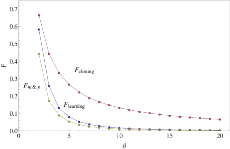
Figure 1: Optimal $1\rightarrow 2$ cloning and learning of a measurement device: we present the values of $F$ for different values of the dimension $d$. The squared dots represent the optimal $1\rightarrow 2$ cloning, the round dots represent the optimal $1\rightarrow 2$ learning and lowest curve corresponds to a strategy in which one performs the optimal estimation followed by the preparation of the estimated measurement.

VII Conclusions

In the present paper we focused on $1\rightarrow 2$ cloning and $1\rightarrow 2$ learning of von Neumann measurements. Even though both problems can be easily formulated in the usual language of quantum mechanics, the necessity to handle the measurement outcome in the remaining part of the scheme makes the optimization complicated and requires suitable mathematical tools. We represented the unknown measurement to be replicated as a measure&prepare channel and we employed framework of quantum combs to perform the network optimization. Thanks to symmetries of the figure of merit the problem was simplified and solved for arbitrary dimension of the measurement’s Hilbert space $d$. In section (V.1) we proposed a realization of optimal $1\rightarrow 2$ cloning of measurements. The proposed scheme has some similarities to optimal cloning of unitary transformations, since they both begin by the control-swap operation, which reflects the presence of quantum parallelism. In this paper we expolit the measure&prepare representation of von Neumann measurement that allowed us to deal with feed forward of classical information in quantum networks. These tool could be in principle used to tackle other quantum information processing tasks in which classical information is involved e.g. estimation and cloning of quantum instruments.

References

(1) W. K Wootters, W. H Zurek, Nature 299, p. 802
(1982).
(2)
M. Nielsen and I. Chuang,
Phys. Rev. Lett. 79, 321 324 (1997)
(3)
V. Bužek and M. Hillery,
Phys. Rev. A 54, 1844 1852 (1996)
(4)
R. F. Werner,
Phys. Rev. A 58, 1827 1832 (1998)
(5)
H. Barnum, C. M. Caves, C. A. Fuchs, R. Jozsa, B. Schumacher
Phys. Rev. Lett. 76 2818-2821 (1996)
(6)
G. M. D’Ariano, C. Macchiavello, P. Perinotti
Phys. Rev. Lett. 95, 060503 (2005)
(7)
V. Scarani, S. Iblisdir, N. Gisin, and A. Acin,
Rev. Mod. Phys. 77, 1225 1256 (2005)
(8)
S. Pirandola, S. Mancini, S. Lloyd and S. L. Braunstein,
Nature Physics 4, 726 (2008)
(9)
K. Bostrom and T. Felbinger, Phys. Rev. Lett. 89, 187902 (2002)
(10)
M. Lucamarini and S. Mancini, Phys. Rev. Lett. 94, 140501 (2005)
(11) G. Chiribella, G. M. D’Ariano, and P. Perinotti,
Phys. Rev. Lett. 101, 180504 (2008).
(12)
A. Ferraro, M. Galbiati, M. G. A. Paris
J. Phys. A 39, L219-L228 (2006)
(13)
A. Bisio, G. M. D’Ariano, P. Perinotti, M. Sedlak,
arXiv:1103.0480v1
(14)
G. Chiribella, G. M. D’Ariano, and P. Perinotti,
Phys. Rev. Lett. 101, 060401 (2008)
(15)
G. Chiribella, G. M. D’Ariano, and P. Perinotti,
Phys. Rev. A 80, 022339 (2009)
(16) A. Bisio, G. Chiribella, G. M. D’Ariano, S.
Facchini, and P. Perinotti, Phys. Rev. A 81, 32324 (2010).
(17)
We omit the derivation of this expression for sake of
simplicity. However it can be derived exploiting the same techniques
as for the derivation of the optimal learning in Sec. VI.