Like-sign dimuon asymmetry of $B^{0}$ meson and LFV
in $SU(5)$ SUSY GUT with $S_{4}$ flavor symmetry

Abstract

The like-sign dimuon charge asymmetry of the $B$ meson, which was reported in the D$\O$ Collaboration, is studied in the $SU(5)$ SUSY GUT model with $S_{4}$ flavor symmetry. Additional CP violating effects from the squark sector are discussed in $B_{s}-\bar{B}_{s}$ mixing process. The predicted like-sign charge asymmetry is in the 2$\sigma$ range of the combined result of D$\O$ and CDF measurements. Since the SUSY contributions in the quark sector affect to the lepton sector because of the $SU(5)$ GUT relation, two predictions are given in the leptonic processes: (i) both ${\rm BR}(\mu\to e\gamma)$ and the electron EDM are close to the present upper bound, (ii) the decay ratios of $\tau$ decays, $\tau\to\mu\gamma$ and $\tau\to e\gamma$, are related to each other via the Cabibbo angle $\lambda_{c}$: ${\rm BR}(\tau\to e\gamma)/{\rm BR}(\tau\to\mu\gamma)\simeq\lambda_{c}^{2}$. These are testable at future experiments.

I Introduction

The CP violation in the $K$ and $B_{d}$ mesons has been well explained within the framework of the standard model (SM). There is one phase, which is a unique source of the CP violation, so called Kobayashi-Maskawa (KM) phase Kobayashi:1973fv , in the quark sector with three families. Until now, the KM phase has successfully described all data related with the CP violation of $K$ and $B_{d}$ systems.

However, there could be new sources of the CP violation if the SM is extended to the supersymmetric (SUSY) models. The CP violating phases appear in soft scalar mass matrices. These contribute to flavor changing neutral currents (FCNC) with the CP violation. Therefore, we should examine carefully CP violating phenomena in the quark sector.

The Tevatron experiments have searched possible effect of the CP violation in the $B$ meson system CDF ; Abazov:2010hj . Recently, the D$\O$ Collaboration reported the interesting result of the like-sign dimuon charge asymmetry $A_{sl}^{b}({\rm D}\O)=-(9.57\pm 2.51\pm 1.46)\times 10^{-3}$ Abazov:2010hj . This result is larger than the SM prediction $A_{sl}^{b}({\rm SM})=(-2.3^{+0.5}_{-0.6})\times 10^{-4}$ Lenz:2006hd at the $3.2\sigma$ level, which indicates an anomalous CP violating phase arising in the $B_{s}$ meson mixing.

Actually, new physics have been discussed to explain the anomalous CP violation in several approaches. As a possibility, new physics contribute to decay width of the $B_{s}$ meson Deshpande:2010hy -Bai:2010kf . Another possibility is to assume new physics does not give additional contribution to the decay width but the $B_{s}-\overline{B}_{s}$ mixing Choudhury:2010ya -Batell:2010qw . This typical model is the general SUSY model with gluino-mediated flavor and CP violation King:2010np ; Endo:2010fk ; Endo:2010yt ; Kubo:2010mh ; Parry:2010ce ; Ko:2010mn ; Wang:2011ax . Relevant mass insertion (MI) parameters and/or squark mass spectrum can explain the anomalous CP violation in the $B_{s}$ system. Since the squark flavor mixing is restricted in $K$ and $B_{d}$ meson systems, the systematic analyses are necessary to clarify the possible effect of squarks.

In this paper, we study the flavor and CP violation within the framework of the non-Abelian discrete symmetry Ishimori:2010au of quark and lepton flavors with SUSY. Then, the flavor symmetry controls the squark and slepton mass matrices as well as the quark and lepton ones. For example, the predicted squark mass matrices reflect structures of the quark mass matrices. Therefore, squark mass matrices provide us an important test for the flavor symmetry.

The non-Abelian discrete symmetry of flavors has been studied intensively in the quark and lepton sectors. Actually, the recent neutrino data analyses Schwetz:2008er -GonzalezGarcia:2010er indicate the tri-bimaximal mixing Harrison:2002er -Harrison:2004uh , which has been at first understood based on the non-Abelian finite group $A_{4}$ Ma:2001dn ; Ma:2002ge ; Ma:2004zv ; Altarelli:2005yp ; Altarelli:2005yx . Until now, much progress has been made in the theoretical and phenomenological analysis of $A_{4}$ flavor model Babu:2002in - Smirnov:2011jv.

An attractive candidate of the flavor symmetry is the $S_{4}$ group, which was successful to explain both quark and lepton mixing  Yamanaka:1981pa-Merlo:2011vc. Especially, $S_{4}$ flavor models to unify quarks and leptons have been proposed in the framework of the $SU(5)$ SUSY GUT  Ishimori:2008fi; Ishimori:2010xk; Hagedorn:2010th; Ding:2010pc, $SO(10)$ SUSY GUT Hagedorn:2006ug; Dutta:2009bj; Patel:2010hr, and the Pati-Salam SUSY GUT Toorop:2010yh; Toorop:2010zg. These unified models seem to explain both mixing of quarks and leptons.

Some of us have studied $S_{4}$ flavor model Ishimori:2010xk, which gives the proper quark flavor mixing angles as well as the tri-bimaximal mixing of neutrino flavors. Especially, the Cabibbo angle is predicted to be $15^{\circ}$ due to $S_{4}$ Clebsch-Gordan coefficients. Including the next-to-leading corrections of the $S_{4}$ symmetry, the predicted Cabibbo angle is completely consistent with the observed one.

We give the squark mass matrices in our $S_{4}$ flavor model by considering the gravity mediation within the framework of the supergravity theory. We estimate the SUSY breaking in the squark mass matrices by taking account of the next-to-leading $S_{4}$ invariant mass operators as well as the slepton mass matrices. Then, we can predict the CP violation in the $B_{s}$ meson taking account of the constraints of the CP violation of $K$ and $B_{d}$ mesons. We also discuss the squark effect on $b\rightarrow s\gamma$ decay and the chromo–electric dipole moment (cEDM) .

Since our model is based on $SU(5)$ SUSY GUT, we can predict the lepton flavor violation (LFV), e.g., $\mu\rightarrow e\gamma$ and $\tau\rightarrow\mu\gamma$ processes Ishimori:2010su. In particular, the $\tau\rightarrow\mu\gamma$ decay ratio reflects the magnitude of the CP violation of the $B_{s}$ meson.

This paper is organized as follows: In section 2, we discuss the possibility of new physics in the framework of the CP violation of the neutral $B$ system. In section 3, we present briefly our $S_{4}$ flavor model of quarks and leptons in $SU(5)$ SUSY GUT, and present the squark and slepton mass matrices. In section 4, we discuss numerically the CP violation of the $B_{s}$ meson with constraints of flavor and CP violations of $K$ and $B_{d}$ mesons. We also discuss the EDM of the electron, cEDM of strange quark and LFV. Section 5 is devoted to the summary. In appendices, we present relevant formulae in order to estimate the flavor violation and the CP violation.

II $B_{s}-\bar{B}_{s}$ Mixing

In this section, we briefly discuss the theory and experimental results of the CP violation of the neutral $B$ meson system. The effective Hamiltonian ${\cal H}^{q}_{\rm eff}(q=d,s)$ of $B_{q}-\bar{B}_{q}$ system is given in terms of the dispersive (absorptive) part $M^{q}(\Gamma^{q})$ as

$${\cal H}^{q}_{\rm eff}=M^{q}-\frac{i}{2}\Gamma^{q},$$ (1)

where the off-diagonal elements $M_{12}^{q}$ and $\Gamma^{q}_{12}$ are responsible for the $B_{q}-\bar{B}_{q}$ oscillations. The light $(L)$ and heavy $(H)$ physical eigenstates $B^{q}_{L(H)}$ with mass $M^{q}_{L(H)}$ and the decay width $\Gamma^{q}_{L(H)}$ are obtained by diagonalizing the effective Hamiltonian ${\cal H}^{q}_{\rm eff}$. The mass and decay width difference between $B^{q}_{L}$ and $B^{q}_{H}$ are related to the elements of ${\cal H}^{q}_{{\rm eff}}$ as

$$\Delta M_{q}\equiv M^{q}_{H}-M^{q}_{L}=2|M_{12}^{q}|,~{}~{}~{}~{}\Delta\Gamma_{q}\equiv\Gamma_{L}^{q}-\Gamma_{H}^{q}=2|\Gamma_{12}^{q}|\cos\phi_{q},~{}~{}~{}~{}\phi_{q}={\rm arg}(-M_{12}^{q}/\Gamma_{12}^{q}),$$ (2)

where we have used $\Delta\Gamma_{q}\ll\Delta M_{q}$.

The “wrong-sign” charge asymmetry $a_{sl}^{q}$ of $B_{q}\to\mu^{-}X$ decay is defined as

$$a_{sl}^{q}\equiv\frac{\Gamma(\bar{B}_{q}\to\mu^{+}X)-\Gamma(B_{q}\to\mu^{-}X)}{\Gamma(\bar{B}_{q}\to\mu^{+}X)+\Gamma(B_{q}\to\mu^{-}X)}\simeq{\rm Im}\left(\frac{\Gamma_{12}^{q}}{M_{12}^{q}}\right)=\frac{|\Gamma_{12}^{q}|}{|M_{12}^{q}|}\sin\phi_{q}\ .$$ (3)

The like-sign dimuon charge asymmetry $A_{sl}^{b}$ is defined and related with $a_{sl}^{q}$ as Grossman:2006ce

$$A_{sl}^{b}\equiv\frac{N_{b}^{++}-N_{b}^{--}}{N_{b}^{++}+N_{b}^{--}}=(0.506\pm 0.043)a_{sl}^{d}+(0.494\pm 0.043)a_{sl}^{s},$$ (4)

where $N_{b}^{\pm\pm}$ is the number of events of $b\bar{b}\to\mu^{\pm}\mu^{\pm}X$.

The SM prediction of $A^{b}_{sl}$ is given as Lenz:2006hd

$$A_{sl}^{b}({\rm SM})=(-2.3^{+0.5}_{-0.6})\times 10^{-4},$$ (5)

which is calculated from Lenz:2006hd

$$a_{sl}^{d}({\rm SM})=(-4.8^{+1.0}_{-1.2})\times 10^{-4},\quad a_{sl}^{s}({\rm SM})=(2.06\pm 0.57)\times 10^{-5}.$$ (6)

Recently, the D$\O$ collaboration reported $A_{sl}^{b}$ with 6.1 fb${}^{-1}$ data set as Abazov:2010hj

$$A_{sl}^{b}({\rm D}\O)=-(9.57\pm 2.51\pm 1.46)\times 10^{-3},$$ (7)

which shows 3.2 $\sigma$ deviation from the SM prediction of Eq.(5). On the other hand, the result by the CDF collaboration with 1.6 fb${}^{-1}$ data CDF $A_{sl}^{b}({\rm CDF})=(8.0\pm 9.0\pm 6.8)\times 10^{-3}$ is consistent with the SM prediction while it has large errors. Combining these measurements, one can obtain

$$A_{sl}^{b}({\rm CDF+D}\O)=-(8.5\pm 2.8)\times 10^{-3},$$ (8)

which is still 3 $\sigma$ away from the SM prediction.

The D$\O$ Collaboration have performed the direct measurement of $a_{sl}^{s}$ Abazov:2009wg as $a_{sl}^{s}({\rm D}\O)=-(1.7\pm 9.1^{+1.4}_{-1.5})\times 10^{-3}$, which is consistent with the SM prediction because of its large errors. However, if one use the present experimental value of $a_{sl}^{d}$ Abazov:2010hj ; Barberio:2008fa; Asner:2010qj, $a_{sl}^{d}({\rm exp})=-(4.7\pm 4.6)\times 10^{-3}$, one can find that Abazov:2010hj ; Asner:2010qj

$$a_{sl}^{s}=-0.0146\pm 0.0075,$$ (9)

is required to obtain $A_{sl}^{b}({\rm D}\O)$. The central value of the required $|a_{sl}^{s}|$ is about three orders of magnitude larger than the SM prediction $a_{sl}^{s}({\rm SM})$. Combining all results, one can obtain the average value

$$a_{sl}^{s}({\rm average})\simeq-(12.7\pm 5.0)\times 10^{-3},$$ (10)

which is still 2.5 $\sigma$ away from the SM prediction $a_{sl}^{s}({\rm SM})$. Therefore, if the D$\O$ result is confirmed, it is a promising hint of new physics (NP) beyond the SM.

The contribution of NP to the dispersive part of the Hamiltonian is parameterized as

$$M_{12}^{q}=M_{12}^{q,SM}+M_{12}^{q,NP}=M_{12}^{q,SM}\left(1+h_{q}e^{2i\sigma_{q}}\right)=M_{12}^{q,SM}\Delta_{q},\quad\Delta_{q}=\left|\Delta_{q}\right|e^{i\phi_{\Delta q}},$$ (11)

where the SM contribution $M_{12}^{q,SM}$ is given by

$$M_{12}^{q,SM}=\frac{G_{F}^{2}M_{B_{q}}}{12\pi^{2}}M_{W}^{2}(V_{tb}V^{*}_{tq})^{2}\hat{\eta}_{B}S_{0}(x_{t})f^{2}_{B_{q}}B_{q},$$ (12)

with parameters listed in Table 1.

Input		Input
$f_{B_{s}}$	$(231\pm 3\pm 15)~{}{\rm MeV}$	$B_{s}(m_{b})$	$0.841\pm 0.013\pm 0.020$
$f_{B_{s}}/f_{B_{d}}$	$1.209\pm 0.007\pm 0.023$	$B_{s}/B_{d}$	$1.01\pm 0.01\pm 0.03$
$\hat{\eta}_{B}$	$0.8393\pm 0.0034$	$S_{0}(x_{t})$	$2.35$
$M_{s}$	$5.3663\pm 0.0006$ GeV	$\Delta M_{s}^{\rm exp}$	$17.77\pm 0.10\pm 0.07~{}\mbox{ps}^{-1}$
$M_{d}$	$5.27917\pm 0.00029$ GeV	$\Delta M_{d}^{\rm exp}$	$0.507\pm 0.005~{}\mbox{ps}^{-1}$
$m_{d}(m_{b})$	$(5.1\pm 1.3)\times 10^{-3}$ GeV	$m_{s}(m_{b})$	$0.085\pm 0.017$ GeV
$m_{b}(m_{b})$	$4.248\pm 0.051$ GeV	$\Delta\Gamma_{s}^{SM}$	$(0.096\pm 0.039)~{}{\rm ps}^{-1}$
$\phi_{d,SM}$	$\left(-10.1^{+3.7}_{-6.3}\right)\times 10^{-2}$	$\phi_{s,SM}$	$\left(+7.4^{+0.8}_{-3.2}\right)\times 10^{-3}$
$|\Gamma_{12}^{s,SM}|/|M_{12}^{s,SM}|$	$(4.97\pm 0.94)\times 10^{-3}$	$\Delta\Gamma_{d}^{SM}/\Delta M_{d}^{SM}$	$(52.6^{+11.5}_{-12.8})\times 10^{-4}$

Table 1: Parameters of the neutral $B$ meson mixing and quark masses Lenz:2006hd ; Lenz:2010gu.

Using these parameters, the mass difference of $B_{q}$ meson, $\Delta M_{q}$, is given by

$$\Delta M_{q}=\Delta M_{q}^{SM}\left|1+h_{q}e^{2i\sigma_{q}}\right|=\Delta M_{q}^{SM}\left|\Delta_{q}\right|.$$ (13)

Since the SM contribution to the absorptive part $\Gamma_{12}^{s}$ is dominated by tree-level decay $b\to c\bar{c}s$, one can set $\Gamma_{12}^{s}=\Gamma_{12}^{s,SM}$. In this case, the wrong-sign charge asymmetry $a_{sl}^{s}$ is written as

$$a_{sl}^{q}=\frac{|\Gamma_{12}^{q,SM}|}{|M_{12}^{q,SM}|}\frac{\sin\left(\phi_{q,SM}+\phi_{\Delta q}\right)}{\left|\Delta_{q}\right|}.$$ (14)

Taking the experimental value $\Delta M_{s}^{\rm exp}$ into account, one finds that $|\Delta_{s}|$ is strongly constrained in the region $|\Delta_{s}|=0.92\pm 0.32$ Lenz:2006hd . Therefore, unphysical condition $\sin(\phi_{s,SM}+\phi_{\Delta s})=-2.56\pm 1.16$ is required to obtain 1 $\sigma$ range of the charge asymmetry (See also Berger:2010wt). Also as discussed in Ref Chen:2010aq, by using the SM prediction of $\Gamma^{d,s}_{12}$ and experimental values of $\Delta M_{d,s}$, they found in model-independent way that the like-sign charge asymmetry is bounded as $-A_{sl}^{b}<3.16\times 10^{-3}$, where the CP violation $S_{J/\psi K_{S}}$ and $S_{J/\psi\phi}$ are also taken into account.

Now we discuss how to avoid this unphysical condition to obtain large charge asymmetry. As the first possibility, one can consider the NP contributions to $\Gamma_{12}^{s}$, which come from additional contributions to decay processes $b\to c\bar{c}s,~{}\tau^{+}\tau^{-}s$, etc. By using the D$\O$ and CDF experimental data of $B_{s}\to J/\psi\phi$ decay CDFD02009, one can subtract $\Delta\Gamma_{s}$ and $\beta_{s}^{J/\psi\phi}\simeq-\phi_{s}/2$ as Barberio:2008fa

$$\Delta\Gamma_{s}=\pm(0.154^{+0.054}_{-0.070})~{}{\rm ps}^{-1},\qquad\beta_{s}^{J/\psi\phi}=(0.39^{+0.18}_{-0.14})~{}{\rm or}~{}(1.18^{+0.14}_{-0.18}),$$ (15)

where the sign of $\Delta\Gamma_{s}$ is still undetermined, and positive (negative) sign corresponds to the first (second) region of $\beta_{s}^{J/\psi\phi}$. Comparing them with the SM predictions, one finds that there still can exist additional contributions to $\Gamma_{12}^{s}$ from NP. This possibility has been studied in several models Deshpande:2010hy ; Oh:2010vc ; He:2010fz ; Dighe:2010nj ; Bauer:2010dga ; Chao:2010mq ; Datta:2010yq ; Bai:2010kf .

In Ref.Choudhury:2010ya , while there are no NP contributions to $\Gamma_{12}^{s}$ in their model, they employed the experimental value of $\Delta\Gamma_{s}$ of Eq.(15) since there must exist theoretical uncertainties. In the $(h_{q},\sigma_{q})$ parametrization of NP, the best fit values of $(h_{s},\sigma_{s})$ are obtained as Ligeti:2010ia

$$(h_{s},\sigma_{s})\simeq(0.5,120^{\circ}),~{}(1.8,100^{\circ}),$$ (16)

by taking $\Delta M_{q},~{}\Delta\Gamma_{q},~{}S_{\psi K}$ and $S_{J/\psi\phi}$ into account, with varying $|\Gamma_{12}^{s}|$ in the range $0-0.3{\rm ps}^{-1}$. In that paper, one can read that the region of $h_{d}\raise 1.29167pt\hbox{$\;<$\kern-7.5pt\raise-4.73611pt\hbox{$\sim\;$}}h_{s}$ is favored as seen in Refs. King:2010np ; Endo:2010fk ; Endo:2010yt .

However in ordinary SUSY models, gluino-squark box diagrams do not give additional contributions to $\Gamma_{12}^{s}$ since such diagrams do not generate additional decay modes of bottom quark. Therefore as the other possibility, constraint for $\Delta M_{q}$ is relaxed in Refs.Kubo:2010mh ; Parry:2010ce . In those papers, they consider models that NP does not give additional contributions to $\Gamma_{12}^{s}$, but to $M_{12}^{q}$. They take a conservative constraint $0.6<\Delta M_{d,s}/\Delta M_{d,s}^{\rm exp}<1.4$ Kubo:2010mh and the UTfit Bona:2008jn allowed region $0.776<\Delta M_{d,s}/\Delta M_{d,s}^{SM}<1.162$ Parry:2010ce . See also Refs. Chen:2010aq; Dobrescu:2010rh ; Ko:2010mn ; Wang:2011ax ; Park:2010sg ; Kostelecky:2010bk for other possibilities.

In this paper, we consider the NP contribution to $B_{s}-\bar{B}_{s}$ mixing by gluino-squark box diagrams in a $SU(5)$ SUSY GUT model with $S_{4}$ flavor symmetry. As shall be discussed in the next section, the soft SUSY breaking terms and related MI parameters $(\delta_{d}^{AB})_{ij}(A,B=L,R)$ obey $S_{4}$ flavor symmetry. In such SUSY models, there are no new contributions to $\Gamma_{12}^{s}$ King:2010np ; Endo:2010fk ; Endo:2010yt ; Kubo:2010mh ; Parry:2010ce ; Ko:2010mn ; Wang:2011ax . While the SUSY contributions to $B_{s}-\bar{B}_{s}$ mixing are induced by $(\delta_{d}^{AB})_{23}$, it is constrained by $b\to s\gamma$ decay. Since the other MI parameters of down-type squark sector are related to $(\delta_{d}^{AB})_{23}$ due to $S_{4}$ symmetry, $K$ and $B_{d}$ meson mixing, which are affected by $(\delta_{d}^{AB})_{12}$ and $(\delta_{d}^{AB})_{13}$, respectively, should also be taken into account. The CP violation in $B_{s}$ meson system is related to cEDM of the strange quark $d^{C}_{s}$ as well. Moreover, the leptonic processes such as $\tau\to\mu\gamma$ affected by $(\delta_{\ell}^{AB})_{23}$ should also be taken into account due to $SU(5)$ GUT relation.

Taking the above processes into account, we assume the following conditions in our numerical calculation: (i) the meson mass differences satisfy

$$0.6<\frac{\Delta M_{d,s}}{\Delta M_{d,s}^{\rm exp}}<1.4,\qquad\frac{|M_{12}^{K,SUSY}|}{\Delta M_{K}^{\rm exp}}<1,\qquad\frac{|{\rm Im}M_{12}^{K,SUSY}|}{\sqrt{2}\Delta M_{K}^{\rm exp}}<\epsilon_{K}=2.2\times 10^{-3},$$ (17)

(ii) cEDM of the strange quark is constrained by the neutron EDM as Hisano:2003iw; Baker:2006ts

$$|ed^{C}_{s}|<1.0\times 10^{-25}~{}e{\rm cm},$$ (18)

(iii) the NP contribution to the branching ratio (BR) of $b\to s\gamma$ is constrained as

$${\rm BR}(b\to s\gamma)^{NP} < 1.0\times 10^{-4}.$$ (19)

While the upper bounds of LFV decay processes $\ell_{i}\to\ell_{j}\gamma$ and the electron EDM are given by Nakamura:2010zzi; Altmannshofer

$${\rm BR}(\mu\to e\gamma) < 1.2\times 10^{-11},\qquad{\rm BR}(\tau\to\mu\gamma)<4.4\times 10^{-8},~{}~{}$$ (20)

$${\rm BR}(\tau\to e\gamma) < 3.3\times 10^{-8},\qquad|ed_{e}|<1.6\times 10^{-27}~{}e{\rm cm},$$ (21)

we do not take these bounds into account in the numerical calculation below. Instead, in the allowed parameter region of our model which can explain the like-sign charge asymmetry, we will obtain the predictions for LFV processes.

We perform numerical analysis in the section IV after introducing the $S_{4}$ flavor model in the next section.

III The $S_{4}$ flavor model

We briefly review $S_{4}$ flavor model of quarks and leptons, which was proposed in Ishimori:2010xk. As the model is based on $SU(5)$ SUSY GUT, it gives sfermion mass matrices as well as quark and lepton mass matrices.

	$(T_{1},T_{2})$	$T_{3}$	$(F_{1},F_{2},F_{3})$	$(N_{e}^{c},N_{\mu}^{c})$	$N_{\tau}^{c}$	$H_{5}$	$H_{\bar{5}}$	$H_{45}$	$\Theta$
$SU(5)$	$10$	$10$	$\bar{5}$	$1$	$1$	$5$	$\bar{5}$	$45$	$1$
$S_{4}$	$\bf 2$	$\bf 1$	$\bf 3$	$\bf 2$	${\bf 1}^{\prime}$	$\bf 1$	$\bf 1$	$\bf 1$	$\bf 1$
$Z_{4}$	$-i$	$-1$	$i$	$1$	$1$	$1$	$1$	$-1$	$1$
$U(1)_{FN}$	$1$	0	0	$1$	0	0	0	0	$-1$

	$(\chi_{1},\chi_{2})$	$(\chi_{3},\chi_{4})$	$(\chi_{5},\chi_{6},\chi_{7})$	$(\chi_{8},\chi_{9},\chi_{10})$	$(\chi_{11},\chi_{12},\chi_{13})$	$\chi_{14}$
$SU(5)$	$1$	$1$	$1$	$1$	$1$	$1$
$S_{4}$	$\bf 2$	$\bf 2$	${\bf 3}^{\prime}$	$\bf 3$	$\bf 3$	$\bf 1$
$Z_{4}$	$-i$	$1$	$-i$	$-1$	$i$	$i$
$U(1)_{FN}$	$-1$	$-2$	0	0	0	$-1$

Table 2: Assignments of $SU(5)$, $S_{4}$, $Z_{4}$, and $U(1)_{FN}$ representations.

III.1 CKM Mixing

In the $SU(5)$ GUT, matter fields are unified into $10$ and $\bar{5}$-dimensional representations as $10\subset(Q,u^{c},e^{c})$ and $\bar{5}\subset(d^{c},L)$. Three generations of $\bar{5}$, which are denoted by $F_{i}~{}(i=1,2,3)$, are assigned to $\bf 3$ of $S_{4}$. On the other hand, the third generation of the $10$-dimensional representation, $T_{3}$, is assigned to $\bf 1$ of $S_{4}$, and the first and second generations of $10$, $(T_{1},T_{2})$, are assigned to $\bf 2$ of $S_{4}$, respectively. Right-handed neutrinos, which are $SU(5)$ gauge singlets, are also assigned to ${\bf 2}$ for the first and second generations, $(N_{e}^{c},N_{\mu}^{c})$, and ${\bf 1}^{\prime}$ for the third one, $N_{\tau}^{c}$. The $5$-dimensional, $\bar{5}$-dimensional, and $45$-dimensional Higgs of $SU(5)$, $H_{5}$, $H_{\bar{5}}$, and $H_{45}$ are assigned to $\bf 1$ of $S_{4}$. In order to obtain desired mass matrices, we introduce $SU(5)$ gauge singlets $\chi_{i}$, so called flavons, which couple to quarks and leptons.

The $Z_{4}$ symmetry is added to obtain relevant couplings. Further, the Froggatt-Nielsen mechanism Froggatt:1978nt is introduced to get the natural hierarchy among quark and lepton masses, as an additional $U(1)_{FN}$ flavor symmetry, where $\Theta$ denotes the Froggatt-Nielsen flavon. The particle assignments of $SU(5)$, $S_{4}$, $Z_{4}$, and $U(1)_{FN}$ are presented in Table 2.

The couplings of flavons with fermions are restricted as follows. At the leading order, $(\chi_{3},\chi_{4})$ are coupled with the right-handed Majorana neutrino sector, $(\chi_{5},\chi_{6},\chi_{7})$ are coupled with the Dirac neutrino sector, $(\chi_{8},\chi_{9},\chi_{10})$ and $(\chi_{11},\chi_{12},\chi_{13})$ are coupled with the charged lepton and down-type quark sectors. At the next-to-leading order, $(\chi_{1},\chi_{2})$ are coupled with the up-type quark sector, and $\chi_{14}$ contributes to the charged lepton and down-type quark sectors, and then the mass ratio of the electron and down quark is reproduced properly.

Our model predicts the quark mixing as well as the tri-bimaximal mixing of leptons. Especially, the Cabibbo angle is predicted to be $15^{\circ}$ at the leading order. The model is consistent with the observed CKM mixing angles and CP violation as well as the non-vanishing $U_{e3}$ of the neutrino flavor mixing.

Let us write down the superpotential respecting $S_{4}$, $Z_{4}$ and $U(1)_{FN}$ symmetries in terms of the $S_{4}$ cutoff scale $\Lambda$, and the $U(1)_{FN}$ cutoff scale $\overline{\Lambda}$. In our calculation, both cutoff scales are taken as the GUT scale which is around $10^{16}$GeV. The $SU(5)$ invariant superpotential of the Yukawa sector up to the linear terms of $\chi_{i}$ ($i=1,\cdots,13$) is given as

$$w =y_{1}^{u}(T_{1},T_{2})\otimes T_{3}\otimes(\chi_{1},\chi_{2})\otimes H_{5}/\Lambda+y_{2}^{u}T_{3}\otimes T_{3}\otimes H_{5}$$

$$\ +y_{1}^{N}(N_{e}^{c},N_{\mu}^{c})\otimes(N_{e}^{c},N_{\mu}^{c})\otimes\Theta^{2}/\bar{\Lambda}$$

$$\ +y_{2}^{N}(N_{e}^{c},N_{\mu}^{c})\otimes(N_{e}^{c},N_{\mu}^{c})\otimes(\chi_{3},\chi_{4})+MN_{\tau}^{c}\otimes N_{\tau}^{c}$$

$$\ +y_{1}^{D}(N_{e}^{c},N_{\mu}^{c})\otimes(F_{1},F_{2},F_{3})\otimes(\chi_{5},\chi_{6},\chi_{7})\otimes H_{5}\otimes\Theta/(\Lambda\bar{\Lambda})$$

$$\ +y_{2}^{D}N_{\tau}^{c}\otimes(F_{1},F_{2},F_{3})\otimes(\chi_{5},\chi_{6},\chi_{7})\otimes H_{5}/\Lambda$$

$$\ +y_{1}(F_{1},F_{2},F_{3})\otimes(T_{1},T_{2})\otimes(\chi_{8},\chi_{9},\chi_{10})\otimes H_{45}\otimes\Theta/(\Lambda\bar{\Lambda})$$

$$\ +y_{2}(F_{1},F_{2},F_{3})\otimes T_{3}\otimes(\chi_{11},\chi_{12},\chi_{13})\otimes H_{\bar{5}}/\Lambda,$$ (22)

where $y_{1}^{u}$, $y_{2}^{u}$, $y_{1}^{N}$, $y_{2}^{N}$, $y_{1}^{D}$, $y_{2}^{D}$, $y_{1}$, and $y_{2}$ are Yukawa couplings of order one, and $M$ is the right-handed Majorana mass, which is taken to be $10^{12}$GeV.

In order to predict the desired quark and lepton mass matrices, we require vacuum alignments for the vacuum expectation values (VEV’s) of flavons. According to the potential analysis, which was presented in Ishimori:2010xk, we have conditions of VEV’s to realize the potential minimum ($V=0$) as follows:

$$(\chi_{1},\chi_{2})=(1,1),\quad(\chi_{3},\chi_{4})=(0,1),\quad(\chi_{5},\chi_{6},\chi_{7})=(1,1,1),\quad(\chi_{8},\chi_{9},\chi_{10})=(0,1,0),$$

$$(\chi_{11},\chi_{12},\chi_{13})=(0,0,1),\quad\chi_{14}^{2}=-\frac{2\eta_{2}}{\eta_{3}}\chi_{1}^{2},$$ (23)

where these magnitudes are given in arbitrary units. Hereafter, we suppose these gauge-singlet scalars develop VEV’s by denoting $\langle\chi_{i}\rangle=a_{i}\Lambda$.

Denoting Higgs doublets as $h_{u}$ and $h_{d}$, we take VEV’s of following scalars by

$$\langle h_{u}\rangle=v_{u},\quad\langle h_{d}\rangle=v_{d},\quad\langle h_{45}\rangle=v_{45},\quad\langle\Theta\rangle=\theta,$$ (24)

which are supposed to be real. We define $\lambda\equiv\theta/\Lambda$ to describe the Froggatt-Nielsen mechanism .

Now, we can write down quark and lepton mass matrices by using the $S_{4}$ multiplication rule in Appendix A. The down-type quark mass matrix at the leading order is given as

$$M_{d}=\begin{pmatrix}0&0&0\\ y_{1}\lambda a_{9}v_{45}/\sqrt{2}&y_{1}\lambda a_{9}v_{45}/\sqrt{6}&0\\ 0&0&y_{2}a_{13}v_{d}\end{pmatrix}.$$ (25)

Then, we have

$$M_{d}^{\dagger}M_{d}=v_{d}^{2}\begin{pmatrix}\frac{1}{2}|\bar{y}_{1}\lambda a_{9}|^{2}&\frac{1}{2\sqrt{3}}|\bar{y}_{1}\lambda a_{9}|^{2}&0\\ \frac{1}{2\sqrt{3}}|\bar{y}_{1}\lambda a_{9}|^{2}&\frac{1}{6}|\bar{y}_{1}\lambda a_{9}|^{2}&0\\ 0&0&|y_{2}|^{2}a_{13}^{2}\end{pmatrix},$$ (26)

where we denote $\bar{y}_{1}v_{d}=y_{1}v_{45}$. This matrix can be diagonalized by the orthogonal matrix $U_{d}^{(0)}$ as

$$U_{d}^{(0)}=\begin{pmatrix}\cos 60^{\circ}&\sin 60^{\circ}&0\\ -\sin 60^{\circ}&\cos 60^{\circ}&0\\ 0&0&1\end{pmatrix}.$$ (27)

The down-type quark masses are given as

$$m_{d}^{2}=0\ ,\quad m_{s}^{2}=\frac{2}{3}|\bar{y}_{1}\lambda a_{9}|^{2}v_{d}^{2}\ ,\quad m_{b}^{2}=|y_{2}|^{2}a_{13}^{2}v_{d}^{2}\ .$$ (28)

The down quark mass vanishes, however tiny masses appear at the next-to-leading order.

The relevant superpotential of down sector at the next-to-leading order is given as

$$\Delta w_{d} =y_{\Delta_{a}}(T_{1},T_{2})\otimes(F_{1},F_{2},F_{3})\otimes(\chi_{1},\chi_{2})\otimes(\chi_{11},\chi_{12},\chi_{13})\otimes H_{\bar{5}}/\Lambda^{2}$$

$$\ +y_{\Delta_{b}}(T_{1},T_{2})\otimes(F_{1},F_{2},F_{3})\otimes(\chi_{5},\chi_{6},\chi_{7})\otimes\chi_{14}\otimes H_{\bar{5}}/\Lambda^{2}$$

$$\ +y_{\Delta_{c}}(T_{1},T_{2})\otimes(F_{1},F_{2},F_{3})\otimes(\chi_{1},\chi_{2})\otimes(\chi_{5},\chi_{6},\chi_{7})\otimes H_{45}/\Lambda^{2}$$

$$\ +y_{\Delta_{d}}(T_{1},T_{2})\otimes(F_{1},F_{2},F_{3})\otimes(\chi_{11},\chi_{12},\chi_{13})\otimes\chi_{14}\otimes H_{45}/\Lambda^{2}$$

$$\ +y_{\Delta_{e}}T_{3}\otimes(F_{1},F_{2},F_{3})\otimes(\chi_{5},\chi_{6},\chi_{7})\otimes(\chi_{8},\chi_{9},\chi_{10})\otimes H_{\bar{5}}\otimes/\Lambda^{2}$$

$$\ +y_{\Delta_{f}}T_{3}\otimes(F_{1},F_{2},F_{3})\otimes(\chi_{8},\chi_{9},\chi_{10})\otimes(\chi_{11},\chi_{12},\chi_{13})\otimes H_{45}\otimes/\Lambda^{2}\ ,$$ (29)

which gives the correction terms in the down-type quark mass matrix.

The down-type quark mass matrix including the next-to-leading order is

$$M_{d}\simeq\begin{pmatrix}\bar{\epsilon}_{11}&\bar{\epsilon}_{21}&\bar{\epsilon}_{31}\\ \frac{\sqrt{3}m_{s}}{2}+\bar{\epsilon}_{12}&\frac{m_{s}}{2}+\bar{\epsilon}_{22}&\bar{\epsilon}_{32}\\ \bar{\epsilon}_{13}&\bar{\epsilon}_{23}&m_{b}+\bar{\epsilon}_{33}\end{pmatrix},$$ (30)

where the explicit forms of $\bar{\epsilon}_{ij}$’s are given in Appendix B, and $m_{s}$ and $m_{b}$ are given in Eq. (28). This mass matrix can be diagonalized by

$$M_{d}^{\rm diag}=V_{d}^{\dagger}M_{d}U_{d}^{(0)}U_{d}^{(1)},$$ (31)

where mixing matrices for left-hand $U_{d}^{(1)}$ and for right-hand $V_{d}$ are estimated as

$$\begin{split}U_{d}^{(1)}&=\begin{pmatrix}1&\theta_{12}^{d}&\theta_{13}^{d}\\ -\theta_{12}^{d}-\theta_{13}^{d}\theta_{23}^{d}&1&\theta_{23}^{d}\\ -\theta_{13}^{d}+\theta_{12}^{d}\theta_{23}^{d}&-\theta_{23}^{d}-\theta_{12}^{d}\theta_{13}^{d}&1\\ \end{pmatrix},\\ V_{d}&=\begin{pmatrix}1&\frac{\tilde{a}}{\lambda}&\tilde{a}\\ -\frac{\tilde{a}}{\lambda}-\tilde{a}^{2}&1&\tilde{a}\\ -\tilde{a}+\frac{\tilde{a}^{2}}{\lambda}&-\tilde{a}-\frac{\tilde{a}^{2}}{\lambda}&1\end{pmatrix},\end{split}$$ (32)

where $\tilde{a}$ denotes the typical value of the square root of the relevant sum of $a_{i}a_{j}$’s as discussed in the next subsection. We neglect CP violating phases then mixing angles $\theta_{12}^{d},\ \theta_{13}^{d},\ \theta_{23}^{d}$ are given as

$$\theta_{12}^{d}=\mathcal{O}\left(\frac{m_{d}}{m_{s}}\right)=\mathcal{O}\left(0.05\right),\ \ \theta_{13}^{d}=\mathcal{O}\left(\frac{m_{d}}{m_{b}}\right)=\mathcal{O}\left(0.005\right),\ \ \theta_{23}^{d}=\mathcal{O}\left(\frac{m_{d}}{m_{b}}\right)=\mathcal{O}\left(0.005\right).$$ (33)

On the other hand, the superpotential of up sector at the next-to-leading order is

$$\Delta w_{u} =y_{\Delta_{a}}^{u}(T_{1},T_{2})\otimes(T_{1},T_{2})\otimes(\chi_{1},\chi_{2})\otimes(\chi_{1},\chi_{2})\otimes H_{5}/\Lambda^{2}$$

$$\ +y_{\Delta_{b}}^{u}(T_{1},T_{2})\otimes(T_{1},T_{2})\otimes\chi_{14}\otimes\chi_{14}\otimes H_{5}/\Lambda^{2}$$

$$\ +y_{\Delta_{c}}^{u}T_{3}\otimes T_{3}\otimes(\chi_{8},\chi_{9},\chi_{10})\otimes(\chi_{8},\chi_{9},\chi_{10})\otimes H_{5}/\Lambda^{2}.$$ (34)

Then the mass matrix becomes

$$M_{u}=v_{u}\begin{pmatrix}2y_{\Delta_{a_{1}}}^{u}a_{1}^{2}+y_{\Delta_{b}}^{u}a_{14}^{2}&y_{\Delta_{a_{2}}}^{u}a_{1}^{2}&y_{1}^{u}a_{1}\\ y_{\Delta_{a_{2}}}^{u}a_{1}^{2}&2y_{\Delta_{a_{1}}}^{u}a_{1}^{2}+y_{\Delta_{b}}^{u}a_{14}^{2}&y_{1}^{u}a_{1}\\ y_{1}^{u}a_{1}&y_{1}^{u}a_{1}&y_{2}^{u}+y_{\Delta_{c}}^{u}a_{9}^{2}\end{pmatrix}.$$ (35)

This symmetric mass matrix is diagonalized by the unitary matrix $U_{u}$ as

$$U_{u}=\begin{pmatrix}\cos 45^{\circ}&\sin 45^{\circ}&0\\ -\sin 45^{\circ}&\cos 45^{\circ}&0\\ 0&0&1\end{pmatrix}\begin{pmatrix}1&0&0\\ 0&r_{t}&r_{c}\\ 0&-r_{c}&r_{t}\end{pmatrix},$$ (36)

where $r_{c}=\sqrt{m_{c}/(m_{c}+m_{t})}$ and $r_{t}=\sqrt{m_{t}/(m_{c}+m_{t})}$.

Therefore, the CKM matrix $V$can be written as

$$V=U_{u}^{\dagger}\begin{pmatrix}1&0&0\\ 0&e^{-i\rho}&0\\ 0&0&1\end{pmatrix}U_{d}^{(0)}U_{d}^{(1)}\ ,$$ (37)

where the phase $\rho$ is an arbitrary parameter originating from complex Yukawa couplings.

At the leading order, the Cabibbo angle is derived as $60^{\circ}-45^{\circ}=15^{\circ}$ and it can be naturally fitted to the observed value by including the next-to-leading order as follows:

$$V_{us} \simeq\theta_{12}^{d}\cos 15^{\circ}+\sin 15^{\circ}.$$ (38)

The $V_{cb}$ and $V_{ub}$ mixing elements are expressed as

$$\begin{split}V_{ud}&\simeq\cos 15^{\circ}-(\theta_{12}^{d}+\theta_{13}^{d}\theta_{23}^{d})\sin 15^{\circ},\\ V_{cb}&\simeq-r_{t}\theta_{13}^{d}e^{i\rho}\sin 15^{\circ}+r_{t}\theta_{23}^{d}e^{i\rho}\cos 15^{\circ}-r_{c}\ ,\\ V_{ub}&\simeq\theta_{13}^{d}\cos 15^{\circ}+\theta_{23}^{d}\sin 15^{\circ},\end{split}$$ (39)

which are consistent with observed values.

We can also predict mass matrices of the charged leptons and neutrinos, which give the tri-bimaximal mixing of leptons. Details are shown in Appendix C.

Since mass eigenvalues of quarks and leptons are give in terms of $a_{i}=\langle\chi_{i}\rangle/\Lambda$, we can estimate $a_{i}$ by putting the observed quark and lepton masses. These are given as

$$a_{3}=a_{8}=a_{10}=a_{11}=a_{12}=0,\qquad a_{1}=a_{2}\simeq\sqrt{\frac{m_{c}}{2\left|y_{\Delta_{a_{2}}}^{u}-\frac{{y_{1}^{u}}^{2}}{y_{2}^{u}}\right|v_{u}}}~{},$$

$$a_{4}=\frac{(y_{1}^{D}\lambda)^{2}(m_{\nu_{3}}-m_{\nu_{1}})m_{\nu_{2}}M}{6y_{2}^{N}{y_{2}^{D}}^{2}m_{\nu_{1}}m_{\nu_{3}}\Lambda},\qquad a_{5}=a_{6}=a_{7}=\frac{\sqrt{m_{\nu_{2}}M}}{\sqrt{3}y_{2}^{D}v_{u}},$$

$$a_{9}=\frac{m_{\mu}}{\sqrt{6}|\bar{y_{1}}|\lambda v_{d}},\qquad a_{13}=\frac{m_{\tau}}{y_{2}v_{d}}\ ,$$ (40)

where masses of quarks and leptons are given at the GUT scale, and the light neutrino masses $m_{\nu_{1,2,3}}$ are given in the Appendix C. Hereafter, we take $\lambda=0.1$ in our calculations.

III.2 Squark and slepton mass matrices

Here we study SUSY breaking terms in the framework of $S_{4}\times Z_{4}\times U(1)_{FN}$ to derive squark and slepton mass matrices. We consider the gravity mediation within the framework of the supergravity theory. We assume that non-vanishing $F$-terms of gauge and flavor singlet (moduli) fields $Z$ and gauge singlet fields $\chi_{i}$ $(i=1,\cdots,14)$ contribute to the SUSY breaking. Their $F$-components are written as

$$F^{\Phi_{k}}=-e^{\frac{K}{2M_{p}^{2}}}K^{\Phi_{k}\bar{I}}\left(\partial_{\bar{I}}\bar{W}+\frac{K_{\bar{I}}}{M_{p}^{2}}\bar{W}\right),$$ (41)

where $M_{p}$ is the Planck mass, $W$ is the superpotential, $K$ denotes the Kähler potential, $K_{\bar{I}J}$ denotes second derivatives by fields, i.e. $K_{\bar{I}J}={\partial}_{\bar{I}}\partial_{J}K$ and $K^{\bar{I}J}$ is its inverse. Here the fields ${\Phi_{k}}$ correspond to the moduli fields $Z$ and gauge singlet fields $\chi_{i}$. The VEV’s of $F_{\Phi_{k}}/\Phi_{k}$ are estimated as $\langle F_{\Phi_{k}}/\Phi_{k}\rangle={\cal O}(m_{3/2})$, where $m_{3/2}$ denotes the gravitino mass, which is obtained as $m_{3/2}=\langle e^{K/2M_{p}^{2}}W/M_{p}^{2}\rangle$.

First, let us study soft scalar masses. Within the framework of the supergravity theory, the soft scalar mass squared is obtained as Kaplunovsky:1993rd

$$m^{2}_{\bar{I}J}K_{{\bar{I}J}}=m_{3/2}^{2}K_{{\bar{I}J}}+|F^{\Phi_{k}}|^{2}\partial_{\Phi_{k}}\partial_{\bar{\Phi_{k}}}K_{\bar{I}J}-|F^{\Phi_{k}}|^{2}\partial_{\bar{\Phi_{k}}}K_{\bar{I}L}\partial_{\Phi_{k}}K_{\bar{M}J}K^{L\bar{M}}.$$ (42)

The invariance under the $S_{4}\times Z_{4}\times U(1)_{FN}$ flavor symmetry as well as the gauge invariance requires the following form of the Kähler potential as

$$K=Z^{(5)}(\Phi)\sum_{i=1,2,3}|F_{i}|^{2}+Z_{(1)}^{(10)}(\Phi)\sum_{i=1,2}|T_{i}|^{2}+Z_{(2)}^{(10)}(\Phi)|R_{\tau}|^{2},$$ (43)

at the lowest level, where $Z^{(5)}(\Phi)$ and $Z_{(1),(2)}^{(10)}(\Phi)$ are arbitrary functions of the singlet fields $\Phi$. By use of Eq. (42) with the Kähler potential in Eq. (43), we obtain the following matrix form of soft scalar masses squared for $\overline{5}\ \overline{5}^{c}$ and ${10}\ {10}^{c}$ combinations, which are denoted as $m_{F}^{2}$ and $m_{T}^{2}$, respectively:

$$(m_{F}^{2})_{ij}=\left(\begin{array}[]{ccc}m_{F}^{2}&0&0\\ 0&m_{F}^{2}&0\\ 0&0&m_{F}^{2}\\ \end{array}\right),\qquad(m_{T}^{2})_{ij}=\left(\begin{array}[]{ccc}m_{T(1)}^{2}&0&0\\ 0&m_{T(1)}^{2}&0\\ 0&0&m_{T(2)}^{2}\\ \end{array}\right).$$ (50)

That is, three right-handed down-type squark and left-handed slepton masses are degenerate, and first two generations of other sectors are degenerate. These predictions would be obvious because the three generations of the $F\subset(d^{c},L)$ fields form a triplet of $S_{4}$, and the $T\subset(Q,u^{c},e^{c})$ fields form a doublet and a singlet of $S_{4}$. These predictions hold exactly before $S_{4}\times Z_{4}\times U(1)_{FN}$ is broken, but its breaking gives next-to-leading terms in the scalar mass matrices.

Next, we study effects due to $S_{4}\times Z_{4}\times U(1)_{FN}$ breaking by $\chi_{i}$. That is, we estimate corrections to the Kähler potential including $\chi_{i}$. Since $(T_{1},T_{2})$ are assigned to ${\bf 2}$ and its conjugate representation is itself ${\bf 2}$. Similarly, $(F_{1},F_{2},F_{3})$ are assigned to ${\bf 3}$ and its conjugation is ${\bf 3}$. Therefore, for the $F_{1,2,3}$ fields, higher dimensional terms are given as

$$\Delta K_{F} =\sum_{i=1,3}Z_{\Delta_{a_{i}}}^{(F)}(\Phi)(F_{1},F_{2},F_{3})\otimes(F_{1}^{c},F_{2}^{c},F_{3}^{c})\otimes(\chi_{i},\chi_{i+1})\otimes(\chi_{i}^{c},\chi_{i+1}^{c})/\Lambda^{2}$$

$$\ +\sum_{i=5,8,11}Z_{\Delta_{b_{i}}}^{(F)}(\Phi)(F_{1},F_{2},F_{3})\otimes(F_{1}^{c},F_{2}^{c},F_{3}^{c})\otimes(\chi_{i},\chi_{i+1},\chi_{i+2})\otimes(\chi_{i}^{c},\chi_{i+1}^{c},\chi_{i+2}^{c})/\Lambda^{2}$$

$$\ +Z_{\Delta_{c}}^{(F)}(\Phi)(F_{1},F_{2},F_{3})\otimes(F_{1}^{c},F_{2}^{c},F_{3}^{c})\otimes\chi_{14}\otimes\chi_{14}^{c}/\Lambda^{2}$$

$$\ +Z_{\Delta_{d}}^{(F)}(\Phi)(F_{1},F_{2},F_{3})\otimes(F_{1}^{c},F_{2}^{c},F_{3}^{c})\otimes\Theta\otimes\Theta^{c}/\bar{\Lambda}^{2}.$$ (51)

For example, higher dimensional terms including $(\chi_{1},\chi_{2})$ and $(\chi_{5},\chi_{6},\chi_{7})$ are explicitly written as

$$\Delta K_{F}^{\left[\chi_{1},\chi_{5}\right]} =Z_{\Delta_{a_{1}}}^{(F)}(\Phi)\left[\frac{\sqrt{2}|\chi_{1}|^{2}}{\Lambda^{2}}(|F_{2}|^{2}-|F_{3}|^{2})\right]$$

$$\ +Z_{\Delta_{b_{5}}}^{(F)}(\Phi)\left[\frac{2|\chi_{5}|^{2}}{\Lambda^{2}}(F_{2}F_{3}^{\ast}+F_{3}F_{2}^{\ast}+F_{1}F_{3}^{\ast}+F_{3}F_{1}^{\ast}+F_{1}F_{2}^{\ast}+F_{2}F_{1}^{\ast})\right].$$ (52)

When we take into account corrections from all $\chi_{i}\chi_{j}^{*}$ to the Kähler potential, the soft scalar masses squared for the $F_{1,2,3}$ fields have the following corrections,

$$(m_{F}^{2})_{ij}=\begin{pmatrix}m_{F}^{2}+\tilde{a}_{F1}^{2}m_{3/2}^{2}&k_{F}a_{5}^{2}m_{3/2}^{2}&k_{F}a_{5}^{2}m_{3/2}^{2}\\ k_{F}a_{5}^{2}m_{3/2}^{2}&m_{F}^{2}+\tilde{a}_{F2}^{2}m_{3/2}^{2}&k_{F}a_{5}^{2}m_{3/2}^{2}\\ k_{F}a_{5}^{2}m_{3/2}^{2}&k_{F}a_{5}^{2}m_{3/2}^{2}&m_{F}^{2}+\tilde{a}_{F3}^{2}m_{3/2}^{2}\end{pmatrix},$$ (53)

where $k_{F}$ is a parameter of order one, and $\tilde{a}_{Fk}^{2}(k=1,2,3)$ are linear combinations of $a_{i}a_{j}$’s.

For the $T_{1,2,3}$ fields, higher dimensional terms are given as

$$\Delta K_{T} =\sum_{i=1,3}Z_{\Delta_{a_{i}}}^{(T)}(\Phi)(T_{1},T_{2})\otimes(T_{1}^{c},T_{2}^{c})\otimes(\chi_{i},\chi_{i+1})\otimes(\chi_{i}^{c},\chi_{i+1}^{c})/\Lambda^{2}$$

$$\ +\sum_{i=5,8,11}Z_{\Delta_{b_{i}}}^{(T)}(\Phi)(T_{1},T_{2})\otimes(T_{1}^{c},T_{2}^{c})\otimes(\chi_{i},\chi_{i+1},\chi_{i+2})\otimes(\chi_{i}^{c},\chi_{i+1}^{c},\chi_{i+2}^{c})/\Lambda^{2}$$

$$\ +Z_{\Delta_{c}}^{(T)}(\Phi)(T_{1},T_{2})\otimes(T_{1}^{c},T_{2}^{c})\otimes\chi_{14}\otimes\chi_{14}^{c}/\Lambda^{2}$$

$$\ +Z_{\Delta_{d}}^{(T)}(\Phi)(T_{1},T_{2})\otimes T_{3}^{c}\otimes(\chi_{1},\chi_{2})/\Lambda^{2}+Z_{\Delta_{e}}^{(T)}(\Phi)(T_{1}^{c},T_{2}^{c})\otimes T_{3}\otimes(\chi_{1}^{c},\chi_{2}^{c})/\Lambda^{2}$$

$$\ +\sum_{i=1,3}Z_{\Delta_{f_{i}}}^{(T)}(\Phi)T_{3}\otimes T_{3}^{c}\otimes(\chi_{i},\chi_{i+1})\otimes(\chi_{i}^{c},\chi_{i+1}^{c})/\Lambda^{2}$$

$$\ +\sum_{i=5,8,11}Z_{\Delta_{g_{i}}}^{(T)}(\Phi)T_{3}\otimes T_{3}^{c}\otimes(\chi_{i},\chi_{i+1},\chi_{i+2})\otimes(\chi_{i}^{c},\chi_{i+1}^{c},\chi_{i+2}^{c})/\Lambda^{2}$$

$$\ +Z_{\Delta_{h}}^{(T)}(\Phi)T_{3}\otimes T_{3}^{c}\otimes\chi_{14}\otimes\chi_{14}^{c}/\Lambda^{2}+Z_{\Delta_{i}}^{(T)}(\Phi)(T_{1},T_{2})\otimes(T_{1}^{c},T_{2}^{c})\otimes\Theta\otimes\Theta^{c}/\bar{\Lambda}^{2}$$

$$\ +Z_{\Delta_{j}}^{(T)}(\Phi)T_{3}\otimes T_{3}^{c}\otimes\Theta\otimes\Theta^{c}/\bar{\Lambda}^{2}.$$ (54)

In the same way, the $T_{1,2,3}$ scalar mass matrix can be written as

$$(m_{T}^{2})_{ij}=\begin{pmatrix}m_{T(1)}^{2}+\tilde{a}_{T11}^{2}m_{3/2}^{2}&\tilde{a}^{2}_{T12}m_{3/2}^{2}&k_{T}a_{1}m_{3/2}^{2}\\ \tilde{a}^{2}_{T12}m_{3/2}^{2}&m_{T(1)}^{2}+\tilde{a}_{T22}^{2}m_{3/2}^{2}&k_{T}a_{1}m_{3/2}^{2}\\ k_{T}^{*}a_{1}m_{3/2}^{2}&k_{T}^{*}a_{1}m_{3/2}^{2}&m_{T(2)}^{2}+\tilde{a}^{2}_{T33}m_{3/2}^{2}\end{pmatrix},$$ (55)

where $k_{T}$ is a complex parameter whose magnitude is of order one, and it is the only new source of the CP violation in our model. The parameters $\tilde{a}_{Tij}^{2}$ are linear combinations of $a_{k}a_{\ell}$’s. In numerical analysis, we use the parameter $\Delta a_{L}$ which is given by $\Delta a_{L}=m_{T(2)}^{2}/m_{T(1)}^{2}-1$.

In order to estimate the magnitude of FCNC phenomena, we move to the super-CKM basis by diagonalizing quark and lepton mass matrices including next-to-leading terms. For the left-handed down-type squark and slepton, we get

$$({\tilde{m}}_{d_{LL}}^{2})_{ij}^{(SCKM)}=U^{\dagger}_{d}(m_{T}^{2})_{ij}U_{d},\quad({\tilde{m}}_{\ell_{LL}}^{2})_{ij}^{(SCKM)}=U^{\dagger}_{E}(m_{F}^{2})_{ij}U_{E},$$ (56)

and for the right-handed down-type squark and slepton as

$$({\tilde{m}}_{d_{RR}}^{2})_{ij}^{(SCKM)}=V^{\dagger}_{d}(m_{F}^{2})_{ij}V_{d},\quad({\tilde{m}}_{e_{RR}}^{2})_{ij}^{(SCKM)}=V^{\dagger}_{E}(m_{T}^{2})_{ij}V_{E},$$ (57)

where the mixing matrices $V_{E}$ and $U_{E}$ are given in Eq. (108) in Appendix C.

Let us study scalar trilinear couplings, i.e. the so called A-terms. The A-terms among left-handed and right-handed squarks (sleptons) and Higgs scalar fields are obtained in the gravity mediation as Kaplunovsky:1993rd

$$h_{IJ}{L}_{J}{R}_{I}H_{K}=\sum_{K={\bar{5}},\ 45}h^{(Y)}_{IJK}{L}_{J}{R}_{I}H_{K}+h^{(K)}_{IJK}{L}_{J}{R}_{I}H_{K},$$ (58)

where

$$h^{(Y)}_{IJK} = F^{\Phi_{k}}\langle\partial_{\Phi_{k}}\tilde{y}_{IJK}\rangle,$$

$$h^{(K)}_{IJK}{L}_{J}{R}_{I}H_{K} = -\langle\tilde{y}_{LJK}\rangle{L}_{J}{R}_{I}H_{K}F^{\Phi_{k}}K^{L\bar{L}}\partial_{\Phi_{k}}K_{\bar{L}I}$$

$$-\langle\tilde{y}_{IMK}\rangle{L}_{J}{R}_{I}H_{d}F^{\Phi_{k}}K^{M\bar{M}}\partial_{\Phi_{k}}K_{\bar{M}J}$$

$$-\langle\tilde{y}_{IJK}\rangle{L}_{J}{R}_{I}H_{K}F^{\Phi_{k}}K^{H_{d}}\partial_{\Phi_{k}}K_{H_{K}},$$

and $K_{H_{K}}$ denotes the Kähler metric of $H_{K}$. In addition, effective Yukawa couplings of the down-type quark $\tilde{y}_{IJK}$ are written as

$$\tilde{y}_{IJK}=y_{1}\begin{pmatrix}0&a_{9}/\sqrt{2}&0\\ 0&a_{9}/\sqrt{6}&0\\ 0&0&0\\ \end{pmatrix}_{LR}+y_{2}\begin{pmatrix}0&0&0\\ 0&0&0\\ 0&0&a_{13}\\ \end{pmatrix}_{LR},$$ (60)

then we have

$$h^{(Y)}_{IJK}=\frac{y_{1}}{\Lambda}\begin{pmatrix}0&\tilde{F}^{a_{9}}/\sqrt{2}&0\\ 0&\tilde{F}^{a_{9}}/\sqrt{6}&0\\ 0&0&0\\ \end{pmatrix}_{LR}+\frac{y_{2}}{\Lambda}\begin{pmatrix}0&0&0\\ 0&0&0\\ 0&0&\tilde{F}^{a_{13}}\\ \end{pmatrix}_{LR},$$ (61)

where $\tilde{F}^{a_{i}}=F^{a_{i}}/a_{i}$ and $\tilde{F}^{a_{i}}/\Lambda={\cal O}(m_{3/2})$.

By use of lowest level of the Kähler potential, we estimate $h^{(K)}_{IJK}$ as

$$h^{(K)}_{IJK}=\tilde{y}_{IJK}(A^{R}_{I}+A^{L}_{J}),$$ (62)

where we assume $A^{L}_{1}=A^{L}_{2}=A^{L}_{3}=F^{\tilde{a}_{i}}/(a_{i}\Lambda)\simeq\mathcal{O}(m_{3/2})$. The magnitudes of $A^{R}_{1}=A^{R}_{2}$ and $A^{R}_{3}$ are also $\mathcal{O}(m_{3/2})$. Furthermore, we should take into account next-to-leading terms of the Kähler potential including $\chi_{i}$. These correction terms appear all entries so that their magnitudes are suppressed in ${\cal O}(\tilde{a})$ compared with the leading term. Then, we obtain

$$(m_{d_{LR}}^{2})_{ij}\simeq(m_{\ell_{LR}}^{2})_{ij}^{\dagger}\simeq m_{3/2}\begin{pmatrix}\tilde{a}_{LR11}^{2}v_{d}&c_{1}\frac{\sqrt{3}m_{s(\mu)}}{2}&\tilde{a}_{LR13}^{2}v_{d}\\ \tilde{a}_{LR21}^{2}v_{d}&c_{1}\frac{m_{s(\mu)}}{2}&\tilde{a}_{LR23}^{2}v_{d}\\ \tilde{a}_{LR31}^{2}v_{d}&\tilde{a}_{LR32}^{2}v_{d}&c_{2}m_{b(\tau)}\end{pmatrix}_{LR},$$ (63)

where $\tilde{a}_{LRij}^{2}$ are linear combinations of $a_{k}a_{\ell}$’s, and $c_{1}$ and $c_{2}$ are of order one parameters. Moving to the super-CKM basis, we have

$$({\tilde{m}}_{{d}_{LR}}^{2})^{(SCKM)}_{ij}=U_{d}^{\dagger}(m_{d_{LR}}^{2})_{ij}V_{d}\simeq m_{3/2}\begin{pmatrix}\mathcal{O}\left(\tilde{a}^{2}v_{d}\right)&\mathcal{O}\left(\tilde{a}^{2}v_{d}\right)&\mathcal{O}\left(\tilde{a}^{2}v_{d}\right)\\ \mathcal{O}\left(\tilde{a}^{2}v_{d}\right)&\mathcal{O}(m_{s})&\mathcal{O}\left(\tilde{a}^{2}v_{d}\right)\\ \mathcal{O}\left(\tilde{a}^{2}v_{d}\right)&\mathcal{O}\left(\tilde{a}^{2}v_{d}\right)&\mathcal{O}(m_{b})\end{pmatrix}.$$ (64)

Similarly, for the charged lepton,

$$({\tilde{m}}_{{\ell}_{LR}}^{2})^{(SCKM)}_{ij}=U_{E}^{\dagger}(m_{\ell_{LR}}^{2})_{ij}V_{E}\simeq m_{3/2}\begin{pmatrix}\mathcal{O}\left(\tilde{a}^{2}v_{d}\right)&\mathcal{O}\left(\tilde{a}^{2}v_{d}\right)&\mathcal{O}\left(\tilde{a}^{2}v_{d}\right)\\ \mathcal{O}\left(\tilde{a}^{2}v_{d}\right)&\mathcal{O}(m_{\mu})&\mathcal{O}\left(\tilde{a}^{2}v_{d}\right)\\ \mathcal{O}\left(\tilde{a}^{2}v_{d}\right)&\mathcal{O}\left(\tilde{a}^{2}v_{d}\right)&\mathcal{O}(m_{\tau})\end{pmatrix}.$$ (65)

III.3 Renormalization group effect

In the framework of the supergravity, soft masses for all scalar particles have the common scale denoted by $m_{\text{SUSY}}$, and gauginos also have the common scale $m_{1/2}$. Therefore, at the GUT scale $m_{\text{GUT}}$, we take

$$M_{1}(m_{\text{GUT}})=M_{2}(m_{\text{GUT}})=M_{3}(m_{\text{GUT}})=m_{1/2}\;.$$ (66)

Effects of the renormalization group running lead at the scale $m_{W}$ to following masses for gauginos,

$$M_{i}(m_{W})\simeq\dfrac{\alpha_{i}(m_{W})}{\alpha_{i}(m_{\text{GUT}})}M_{i}(m_{\text{GUT}}).$$ (67)

Taking into account the renormalization group effect Martin:1993zk on the average mass scale in $m_{e_{L}}^{2}$, $m_{e_{R}}^{2}$, $m_{q_{L}}^{2}$, and $m_{d_{R}}^{2}$ with neglecting Yukawa couplings, we have

$$\begin{split}m_{e_{L}}^{2}(m_{W})&\simeq m_{L}^{2}(m_{\text{GUT}})+0.5M_{2}^{2}(m_{\text{GUT}})+0.04M_{1}^{2}(m_{\text{GUT}})\simeq m_{\text{SUSY}}^{2}+0.54m_{1/2}^{2},\\ m_{e_{R}}^{2}(m_{W})&\simeq m_{R}^{2}(m_{\text{GUT}})+0.15M_{1}^{2}(m_{\text{GUT}})\simeq m_{\text{SUSY}}^{2}+0.15m_{1/2}^{2}\;,\\ m_{q_{L}}^{2}(m_{W})&\simeq m_{R}^{2}(m_{\text{GUT}})+0.004M_{1}^{2}(m_{\text{GUT}})+0.4M_{2}^{2}(m_{\text{GUT}})+3.6M_{3}^{2}(m_{\text{GUT}})\\ &\simeq m_{\text{SUSY}}^{2}+4.1m_{1/2}^{2}\;,\\ m_{d_{R}}^{2}(m_{W})&\simeq m_{R}^{2}(m_{\text{GUT}})+0.015M_{1}^{2}(m_{\text{GUT}})+3.6M_{3}^{2}(m_{\text{GUT}})\simeq m_{\text{SUSY}}^{2}+3.7m_{1/2}^{2}\;.\end{split}$$ (68)

For Yukawa couplings, the $b-\tau$ unification is realized at the leading order in our model, however, the $b-\tau$ unification is deviated when we include the next-to-leading order mass operators due to terms including $H_{45}$, see Ref. Ishimori:2010su for the detail. In that paper, we have calculated the renormalization group equations and observed fermion masses at the weak scale can be obtained when $\tan\beta$ is larger than two. Hereafter, we take $\tan\beta=3$ on the numerical analysis.

IV Numerical Analysis

In this section, we perform numerical analysis to show that the $S_{4}$ flavor model presented in the previous section can explain the like-sign charge asymmetry in the $B_{s}-\bar{B}_{s}$ system. In order for this calculation, we first define the MI parameters for down-type squarks $\delta_{d}^{LL}$, $\delta_{d}^{LR}$, $\delta_{d}^{RL}$, and $\delta_{d}^{RR}$ and for sleptons $\delta_{\ell}^{LL}$, $\delta_{\ell}^{LR}$, $\delta_{\ell}^{RL}$ and, $\delta_{e}^{RR}$ as

$$\begin{split}&m_{\tilde{q}}^{2}\begin{pmatrix}\delta_{d}^{LL}&\delta_{d}^{LR}\\ \delta_{d}^{RL}&\delta_{d}^{RR}\\ \end{pmatrix}=\begin{pmatrix}({\tilde{m}}_{{d}_{LL}}^{2})^{(SCKM)}&({\tilde{m}}_{{d}_{LR}}^{2})^{(SCKM)}\\ ({\tilde{m}}_{{d}_{RL}}^{2})^{(SCKM)}&({\tilde{m}}_{{d}_{RR}}^{2})^{(SCKM)}\\ \end{pmatrix}-\text{diag}(m_{\tilde{q}}^{2})\ ,\\ &m_{\tilde{\ell}}^{2}\begin{pmatrix}\delta_{\ell}^{LL}&\delta_{\ell}^{LR}\\ \delta_{\ell}^{RL}&\delta_{e}^{RR}\\ \end{pmatrix}=\begin{pmatrix}({\tilde{m}}_{{\ell}_{LL}}^{2})^{(SCKM)}&({\tilde{m}}_{{\ell}_{LR}}^{2})^{(SCKM)}\\ ({\tilde{m}}_{{\ell}_{RL}}^{2})^{(SCKM)}&({\tilde{m}}_{{e}_{RR}}^{2})^{(SCKM)}\\ \end{pmatrix}-\text{diag}(m_{\tilde{\ell}}^{2})\ ,\end{split}$$ (69)

where $m_{\tilde{q}}$ and $m_{\tilde{\ell}}$ are average squark and slepton masses with the values given below.

In the numerical analysis, we fix the following parameters

$$m_{3/2} = 430~{}{\rm GeV},~{}m_{\tilde{q}}=880~{}{\rm GeV},~{}m_{\tilde{\ell}}=520~{}{\rm GeV},$$

$$M_{1} = 135~{}{\rm GeV},~{}M_{2}=270~{}{\rm GeV},~{}M_{3}\equiv m_{\tilde{g}}=1~{}{\rm TeV},$$ (70)

which are derived from the universal relation at the GUT scale

$$m_{1/2}(m_{\text{GUT}})=m_{3/2}(m_{\text{GUT}})=m_{\rm SUSY}(m_{\text{GUT}})= 430~{}{\rm GeV},$$ (71)

by through the renormalization group effect discussed in the section III-C. This universal value is taken to be consistent with the lower bound of the gluino mass, which has been reported recently at Atlas Collaboration of LHC Aad:2011hh; daCosta:2011qk; Collaboration:2011ks. For the other parameters, we assume the following regions:

$$\mu = [500,1000]~{}{\rm GeV},~{}\Delta a_{L}=[-0.5,5],~{}|k_{T}a_{1}|=[0,2],~{}{\rm arg}(k_{T}a_{1})=[-\pi,\pi],$$

$$a_{5} = [0,0.001],~{}\tilde{a}_{T12}=[0,0.1],~{}\tilde{a}_{LRij}=[0,0.01],$$ (72)

with $\tan\beta=3,~{}c_{1,2}=1,$ and $k_{F}=1$. In Eq.(72), the number of left-handed and right-handed sides in braces denote the minimal and maximal values, respectively. In our calculation, we neglect the diagonal elements of scalar masses $\tilde{a}_{F(1,2,3)}$ and $\tilde{a}_{T(11,22,33)}$. The leading contribution to the parameters $\tilde{a}$ in the soft-terms are $a_{1}$ as $\tilde{a}_{LRij}\simeq\sqrt{a_{1}a_{5}}$ and $\tilde{a}_{T12}\simeq a_{1}$. As given in Appendix D, the SUSY contribution to $M_{12}^{s,SUSY}$ is estimated as

$$M_{12}^{s,SUSY}\simeq-\frac{\alpha_{S}^{2}}{216m_{\tilde{q}}^{2}}\frac{2}{3}M_{B_{s}}f_{B_{s}}^{2}\Bigl{\{}-0.59\left[(\delta_{d}^{LL})^{2}_{23}+(\delta_{d}^{RR})^{2}_{23}\right]+31(\delta_{d}^{LL})_{23}(\delta_{d}^{RR})_{23}$$

$$-9.4\left[(\delta_{d}^{LR})^{2}_{23}+(\delta_{d}^{RL})^{2}_{23}\right]+7.9(\delta_{d}^{LR})_{23}(\delta_{d}^{RL})_{23}\Bigr{\}},$$ (73)

for $x=m_{\tilde{g}}^{2}/m_{\tilde{q}}^{2}\simeq 1.3$, and similar for $B_{d}$ mixing. The coefficients in front of MI parameters for $K$ meson mixing are $-0.59,554,-183,114$, respectively. Since the $LR$ terms $(\delta^{LR,RL}_{d})_{ij}$ are strictly constrained by $b\to s\gamma$ as seen in Appendix D, the $(\delta_{d}^{LL(RR)})_{ij}$ terms gives larger contribution to $M_{12}^{s,SUSY}$. Among them, since $(\delta_{d}^{RR})_{ij}\simeq k_{F}a_{5}^{2}\raise 1.29167pt\hbox{$\;<$\kern-7.5pt\raise-4.73611pt\hbox{$\sim\;$}}10^{-6}$ in our parameter region given in Eq.(72), the first term $(\delta_{d}^{LL})_{ij}^{2}$ gives the dominant contributions. The approximation form of the $LL$ parameters $(\delta_{d}^{LL})_{ij}$ are given by

$$(\delta_{d}^{LL})_{12} \simeq \theta_{13}^{d}\theta_{23}^{d}\Delta a_{L}-\frac{m_{3/2}^{2}}{m_{\tilde{q}}^{2}}\left(\theta_{13}^{d}\frac{1+\sqrt{3}}{2}k_{T}^{*}a_{1}+\theta_{23}^{d}\frac{1-\sqrt{3}}{2}k_{T}a_{1}\right)$$ (74)

$$\simeq -\frac{m_{3/2}^{2}}{m_{\tilde{q}}^{2}}\sqrt{2}\left(\theta^{d}_{13}V_{ud}k_{T}^{*}a_{1}-\theta_{23}^{d}V_{us}k_{T}a_{1}\right),$$

$$(\delta_{d}^{LL})_{13} \simeq -\theta_{13}^{d}\Delta a_{L}+\frac{m_{3/2}^{2}}{m_{\tilde{q}}^{2}}\left(\frac{1-\sqrt{3}}{2}-\theta_{12}^{d}\frac{1+\sqrt{3}}{2}\right)k_{T}a_{1}\simeq-\frac{m_{3/2}^{2}}{m_{\tilde{q}}^{2}}\sqrt{2}V_{us}k_{T}a_{1},$$ (75)

$$(\delta_{d}^{LL})_{23} \simeq -\theta_{23}^{d}\Delta a_{L}+\frac{m_{3/2}^{2}}{m_{\tilde{q}}^{2}}\left(\frac{1+\sqrt{3}}{2}+\theta_{12}^{d}\frac{1-\sqrt{3}}{2}\right)k_{T}a_{1}\simeq\frac{m_{3/2}^{2}}{m_{\tilde{q}}^{2}}\sqrt{2}V_{ud}k_{T}a_{1},$$ (76)

where in the last approximation of each expression, we have neglected the first term proportional to $\theta_{13,23}^{d}\simeq 0.005$ and $\Delta a_{L}\sim 1$. Notice that the MI parameters are expressed in terms of the CKM elements, and that both $(\delta_{d}^{LL})_{13}$ and $(\delta_{d}^{LL})_{23}$ have the same phase structure $k_{T}a_{1}$, which is only the new source of the CP violation in our model. These are the typical feature of our $S_{4}$ flavor model. By using these expressions, one finds that the $K^{0}-\bar{K}^{0}$ mixing induced by $(\delta_{d}^{LL})_{12}$ is more suppressed by additional factor $\theta_{ij}^{d}$.

The cEDM for the strange quark is estimated from the formula in Appendix D as

$$ed^{C}_{s}\sim 10^{-20}\text{Im}[(\delta_{d}^{LL})_{23}(\delta_{d}^{LR})_{33}(\delta_{d}^{RR})_{32}]~{}e{\rm cm}\sim 10^{-28}{\rm Im}[(\delta_{d}^{LL})_{23}]~{}e{\rm cm},$$ (77)

for $x\simeq 1.3$, $(\delta_{33}^{d})_{LR}\sim 10^{-2}$ and $(\delta_{32}^{d})_{RR}\sim 10^{-6}$. Therefore, $(\delta_{23}^{d})_{LL}$ is not constrained by cEDM. As for the $b\to s\gamma$ process, one can see that $(\delta^{d}_{23})_{LR}$ should be strongly suppressed while $(\delta^{d}_{23})_{LL,RR}$ have an additional suppression factor $m_{b}/m_{\tilde{g}}\sim 10^{-3}$. In our numerical calculation, we take $\tilde{a}_{LRij}\raise 1.29167pt\hbox{$\;<$\kern-7.5pt\raise-4.73611pt\hbox{$\sim\;$}}0.01$ so that $b\to s\gamma$ is well suppressed, and the allowed region of $|(\delta^{LL}_{d})_{23}|$ is also small enough as mentioned below.

First we discuss the allowed regions of the parameters $(h_{s},h_{d}),~{}(h_{s},\sigma_{s}),~{}(h_{d},\sigma_{d})$ defined in Eq.(11). In our model, the parameters $h_{d,s}e^{2i\sigma_{d,s}}$ are estimated as

$$h_{d}e^{2i\sigma_{d}} = \frac{M_{12}^{d,SUSY}}{M_{12}^{d,SM}}\simeq(27-i25)(\delta_{d}^{LL})_{13}^{2},~{}$$ (78)

$$h_{s}e^{2i\sigma_{s}} = \frac{M_{12}^{s,SUSY}}{M_{12}^{s,SM}}\simeq(1.7+i0.06)(\delta_{d}^{LL})_{23}^{2},$$ (79)

where the MI parameters $(\delta_{d}^{LL})_{ij}$ reflect the flavor symmetry, while the factors $(27-i25)$ and $(1.7+i0.06)$ do not. The ratio of $(27-i25)/(1.7+i0.06)$ is related to the CKM elements as $(27-i25)/(1.7+i0.06)\simeq M_{12}^{s,SM}/M_{12}^{d,SM}\simeq(V_{ts}^{*}/V_{td}^{*})^{2}$. We obtain the ratio of $h_{d}$ and $h_{s}$ as

$$\frac{h_{d}}{h_{s}}\simeq\frac{|27-i25|}{|1.7+i0.06|}\frac{|V_{us}|^{2}}{|V_{ud}|^{2}}\simeq\frac{|V_{ts}|^{2}}{|V_{td}|^{2}}\frac{|V_{us}|^{2}}{|V_{ud}|^{2}}\simeq 1.$$ (80)

Therefore, the fact that the region $h_{d}\simeq h_{s}$ is favored reflects the flavor structure of the $S_{4}$ flavor model. The CP violation phase $\phi_{s}$ is given by

$$\phi_{s}\simeq{\rm arg}\left[-(1+h_{s}e^{2i\sigma_{s}})\right],$$ (81)

with neglecting the SM contribution. The CP phase $\sin\phi_{s}$ is bounded as $|\sin\phi_{s}|\raise 1.29167pt\hbox{$\;<$\kern-7.5pt\raise-4.73611pt\hbox{$\sim\;$}}h_{s}$ for $h_{s}<1$, and has the negatively-maximal value $\sin\phi_{s}\simeq-h_{s}$ at $\sigma_{s}\simeq 120^{\circ}$. This corresponds to the best-fit value $(h_{s},\sigma_{s})=(0.5,120^{\circ})$ of Eq.(16)Ligeti:2010ia.

Fig.1 shows the plot in the $\phi_{s}-A_{sl}^{b}$ plane. The horizontal and vertical lines are the experimental values of one-dimensional likelihood analysis CDF2010

$$\phi_{s}=[-1.8,0.4]~{}({\rm rad}),~{}{\rm at}~{}95\%~{}{\rm C.L.},$$ (82)

and 2$\sigma$ range of $A_{sl}^{b}$ in Eq.(8), respectively. The blue (dark gray) and orange (light gray) regions denote 2$\sigma$ and 3$\sigma$ regions of $A_{sl}^{b}$ in Eq.(8), respectively. By using Eq.(14) and $|1+h_{s}{\rm exp}({2i\sigma_{s}})|\sim(1+0.5{\rm exp}[2i120^{\circ}])\simeq 0.8$, we obtain $-a_{sl}^{s}\raise 1.29167pt\hbox{$\;>$\kern-7.5pt\raise-4.73611pt\hbox{$\sim\;$}}10^{-3}$, and similar for $a_{sl}^{d}$. As a consequence we obtain the like-sign charge asymmetry as $-A_{sl}^{b}\raise 1.29167pt\hbox{$\;>$\kern-7.5pt\raise-4.73611pt\hbox{$\sim\;$}}10^{-3}$, which is within 2$\sigma$ range of $A_{sl}^{b}$ of Eq.(8).

Fig.2 shows the allowed region in the ${\rm Re}(\delta_{d}^{LL})_{23}-{\rm Im}(\delta_{d}^{LL})_{23}$ plane. One finds from Eq.(79) that in order to obtain the best fit value $(h_{s},\sigma_{s})=(0.5,120^{\circ})$, the sign of ${\rm Re}(\delta_{d}^{LL})_{23}$ and ${\rm Im}(\delta_{d}^{LL})_{23}$ must be opposite from each other, with ${\rm Re}(\delta_{d}^{LL})_{23}\simeq\pm 0.3$ and ${\rm Im}(\delta_{d}^{LL})_{23}\simeq\mp 0.4$. This allowed region $|(\delta_{d}^{LL})_{23}|\raise 1.29167pt\hbox{$\;<$\kern-7.5pt\raise-4.73611pt\hbox{$\sim\;$}}0.5$ is small enough to suppress $b\to s\gamma$. The similar figure is drawn in the ${\rm Re}(\delta_{d}^{LL})_{13}-{\rm Im}(\delta_{d}^{LL})_{13}$ plane with $|V_{td}/V_{ts}|\simeq 0.22$ times smaller area.

Figure 1: Allowed region in the $\phi_{s}-A_{sl}^{b}$ plane. The blue (dark gray) and orange (light gray) regions denote 2$\sigma$ and 3$\sigma$ regions of $A_{sl}^{b}$ in Eq. (8). The blue (black) error bars of the horizontal and vertical lines are experimental values of $2\sigma$ region of $\phi_{s}$ and $A_{sl}^{b}$.

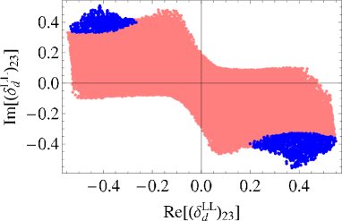
Figure 2: Allowed region in the ${\rm Re}(\delta_{d}^{LL})_{23}-{\rm Im}(\delta_{d}^{LL})_{23}$ plane. The blue (dark gray) and orange (light gray) regions denote 2$\sigma$ and 3$\sigma$ regions of $A_{sl}^{b}$ in Eq. (8).

Figure 3: Allowed region in the $(a_{sl}^{s}-a_{sl}^{d})-\phi_{s}$ plane. The blue (dark gray) and orange (light gray) regions denote 2$\sigma$ and 3$\sigma$ regions of $A_{sl}^{b}$ in Eq. (8). The blue error bars of the horizontal and vertical lines are experimental values of $2\sigma$ region of $\phi_{s}$ and $(a_{sl}^{s}-a_{sl}^{d})$. The horizontal line is experimental values of 2$\sigma$ region for $\phi_{s}$, and the vertical line is the SM prediction of $(a_{\text{sl}}^{s}-a_{\text{sl}}^{d})$.

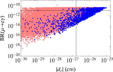
Figure 4: Allowed region in the $|d_{e}|-BR(\mu\to e\gamma)$ plane. The blue (dark gray) and orange (light gray) regions denote 2$\sigma$ and 3$\sigma$ regions of $A_{sl}^{b}$ in Eq. (8). The horizontal and vertical lines are experimental bounds of $|d_{e}|$ and $BR(\mu\to e\gamma)$.

In Fig.3, we predict the difference $a_{sl}^{s}-a_{sl}^{d}$, which will be measured at LHCb, as a function of $\phi_{s}$. The SM prediction Nierste:2011ti $a_{sl}^{s,SM}-a_{sl}^{d,SM}=(4.3\pm 0.7)\times 10^{-4}$ is also shown. We predict that $a_{sl}^{s}-a_{sl}^{d}\simeq(1-5)\times 10^{-3}$ in the 2$\sigma$ region of $A_{sl}^{b}$. This will be a good test for our $S_{4}$ flavor model.

Since our model is based on the $SU(5)$ GUT, above contributions in the quark sector affect to the lepton sector. Therefore, sleptons contribute to the LFV processes and EDM of the electron Borzumati:1986qx; Hisano:1995nq, in which the experimental measurements give the upper bounds Adam:2009ci; Regan:2002ta; DeMille. The Fig.4 shows the relation of ${\rm BR}(\mu\to e\gamma)$ and the electron EDM. Within the MI parameters, $(\delta_{e}^{RR})_{ij}\sim(\delta_{d}^{LL})_{ji}$ except for $(i,j)=(1,2),(2,1)$ are relatively large in our model. Therefore one finds from Appendix E that the $(\delta_{e}^{RL})_{21}$ term in $A_{L}^{21}$, which is enhanced by $M_{1}/m_{\mu}\sim 10^{3}$, mainly contributes to $\mu\to e\gamma$ process. As for the electron EDM, the terms with one small MI parameters dominates. The largest contributions are approximately estimated as

$${\rm BR}(\mu\to e\gamma) \simeq \frac{48\pi^{3}\alpha}{G_{F}^{2}}\left|\frac{\alpha_{1}}{4\pi}\frac{(\delta_{e}^{RL})_{21}}{m_{\tilde{\ell}}^{2}}\left(\frac{M_{1}}{m_{\mu}}\right)2f_{2n}(x_{1})\right|^{2}$$ (83)

$$\simeq 3\times 10^{-11}\left(\frac{520{\rm GeV}}{m_{\tilde{\ell}}}\right)^{4}\left(\frac{M_{1}}{135{\rm GeV}}\right)^{2}\left(\frac{|(\delta_{e}^{RL})_{21}|}{10^{-5}}\right)^{2},$$

$$|d_{e}/e| \simeq \frac{\alpha_{1}}{4\pi}\frac{M_{1}}{m_{\tilde{\ell}}^{2}}\Bigl{|}{\rm Im}[(\delta_{\ell}^{LR})_{13}(\delta_{e}^{RR})_{31}]f_{3n}(x_{1})$$ (84)

$$+ {\rm Im}[(\delta_{\ell}^{LR})_{12}(\delta_{e}^{RR})_{23}(\delta_{e}^{RR})_{31}+(\delta_{\ell}^{LR})_{13}(\delta_{e}^{RR})_{33}(\delta_{e}^{RR})_{31}]f_{4n}(x_{1})\Bigr{|}$$

$$\simeq 1\times 10^{-26}cm\times\left(\frac{M_{1}}{135{\rm GeV}}\right)\left(\frac{520{\rm GeV}}{m_{\tilde{\ell}}}\right)^{2}\Bigl{[}\left(\frac{(\delta_{\ell}^{LR})_{13}}{10^{-5}}\right)\left(\frac{(\delta_{e}^{RR})_{31}}{0.1}\right)+\cdots\Bigr{]}.$$

The value of $|(\delta_{e}^{RL})_{ij}|$ is of order $m_{3/2}v_{d}/m_{\tilde{\ell}}^{2}\times\tilde{a}_{LRij}^{2}\raise 1.29167pt\hbox{$\;<$\kern-7.5pt\raise-4.73611pt\hbox{$\sim\;$}}10^{-5}$. Therefore we find that ${\rm BR}(\mu\to e\gamma)$ and electron EDM can be close to the present experimental bound as shown in the figure.

The $b-s$ transition by $(\delta_{d}^{LL})_{23}$ in the quark sector simultaneously induce the LFV $\tau$ decay $\tau\to\mu\gamma$ by $(\delta_{e}^{RR})_{32}$. The dominant contribution is estimated from Appendix E as

$${\rm BR}(\tau\to\mu\gamma) \simeq {\rm BR}(\tau\to\mu\nu_{\tau}\bar{\nu}_{\mu})\frac{48\pi^{3}\alpha}{G_{F}^{2}}\left(\frac{\alpha_{1}}{4\pi}\right)^{2}\left[\frac{(\delta_{e}^{RR})_{32}}{m_{\tilde{\ell}}^{2}}\mu M_{1}\tan\beta\left(\frac{f_{3n}(x_{1})}{m_{\tilde{\ell}}^{2}}-\frac{2f_{2n}(x_{1},x_{\mu})}{\mu^{2}-M_{1}^{2}}\right)\right]^{2}$$ (85)

$$\simeq 10^{-8}\left(\frac{520{\rm GeV}}{m_{\tilde{\ell}}}\right)^{8}\left(\frac{M_{1}}{135{\rm GeV}}\right)^{2}\left(\frac{\tan\beta}{3}\right)^{2}\left(\frac{\mu}{500{\rm GeV}}\right)^{2}|(\delta_{e}^{RR})_{32}|^{2},$$

and similar for $\tau\to e\gamma$ decay. Therefore for large $\mu$ term, $\tau\to\mu\gamma$ can be close to present upper bound given in Eq.(21). By using the expression Eqs.(75) and (76), we obtain the relation of ${\rm BR}(\tau\to\mu\gamma)$ and ${\rm BR}(\tau\to e\gamma)$ depending on the Cabibbo angle $\lambda_{c}\simeq 0.22$ as follows:

$$\frac{{\rm BR}(\tau\to e\gamma)}{{\rm BR}(\tau\to\mu\gamma)}\simeq\frac{|(\delta_{e}^{RR})_{31}|^{2}}{|(\delta_{e}^{RR})_{32}|^{2}}\simeq\frac{|(\delta_{d}^{LL})_{13}|^{2}}{|(\delta_{d}^{LL})_{23}|^{2}}\simeq\frac{|V_{us}|^{2}}{|V_{ud}|^{2}}\simeq\lambda_{c}^{2}\simeq 0.05.$$ (86)

Therefore we conclude that there exist the parameter region which can explain the like-sign dimuon asymmetry $A_{sl}^{b}$ in the $S_{4}$ flavor model, and in this case we predict that the LFV $\tau\to\mu\gamma$ decay can be so large that future experiments will reach, and the ratio of LFV of $\tau$ decays, $\tau\to e\gamma$ and $\tau\to\mu\gamma$, depends on the Cabibbo angle $\lambda_{c}$.

V Summary

Recently the D$\O$ Collaboration reported the like-sign dimuon charge asymmetry $A_{sl}^{b}$ in $b\bar{b}\to\mu^{\pm}\mu^{\pm}X$ decay processes. Their result shows 3.2$\sigma$ deviation from the standard model prediction. One promising interpretation of this result is that there exist additional contribution of new physics to the CP violation in $B_{s}-\bar{B}_{s}$ mixing process. In the effective Hamiltonian of the neutral $B_{s}$ meson system, there are three physical quantities $|\Gamma_{12}^{s}|$, $|M_{12}^{s}|$ and the CP phase $\phi_{s}={\rm arg}(-M_{12}^{s}/\Gamma_{12}^{s})$. In order to obtain large CP asymmetry in the neutral $B_{s}$ meson system, additional contributions from new physics to at least one of these three quantities are required. Within these possibilities, one can consider new physics that the absorptive part $\Gamma_{12}^{s}$ can be enhanced. However in general supersymmetric models, the gluino-squark box diagrams give the dominant contributions to $B_{s}-\bar{B}_{s}$ mixing, which do not affect $|\Gamma_{12}^{s}|$. Therefore in those models, new physics contributes to $|M_{12}^{s}|$ and $\phi_{s}$.

In this paper we have considered an $SU(5)$ SUSY GUT with $S_{4}$ flavor symmetry. In this model, the Cabibbo angle, $\lambda_{c}\sim\sin 15^{\circ}$, of the quark sector is given by a difference of $45^{\circ}$ from up sector and $60^{\circ}$ from down sector due to the Clebsch-Gordan coefficients at the leading order. As for the lepton sector, the tri-bimaximal form is generated in neutrino sector. These are consequences of the $S_{4}$ flavor symmetry. Since the matter multiplet $T(10)$ and $F(\bar{5})$ are embedded into ${\bf 2}+{\bf 1}$ and ${\bf 3}$ of the $S_{4}$ group, respectively, the scalar masses of right-handed down-type squark and left-handed slepton are degenerated at the leading order, while those of $T_{1,2,3}$ fields are degenerated in the first two generations. Moreover for scalar mass matrix of $T_{1,2,3}$ fields, the relation $(m^{2}_{T})_{13}=(m^{2}_{T})_{23}\propto k_{T}a_{1}$ holds due to the $S_{4}$ symmetry. The factor $k_{T}a_{1}$ in the scalar mass matrix is assumed to be the only additional complex parameter in our model, which is responsible for the CP violation in the neutral $B_{s}$ meson system via gluino-squark box diagrams. As a consequence, the mass-insertion parameters $(\delta_{d}^{LL})_{13}$ and $(\delta_{d}^{LL})_{23}$ have approximately the structure of $V_{us}k_{T}a_{1}$ and $V_{ud}k_{T}a_{1}$, respectively.

We have shown that the like-sign charge asymmetry $A_{sl}^{b}$ is in the 2$\sigma$ range of the combined result of D$\O$ and CDF measurements. Since the relation between two CP phases $\sin\phi_{d}\simeq\sin\phi_{s}$ holds due to $S_{4}$ flavor symmetry, and it can be large, we obtain large wrong-sign and like-sign asymmetry: $|a_{sl}^{d,s}|\sim|A_{sl}^{b}|\sim 10^{-3}$. The SUSY contributions in the quark sector affect to the lepton sector because of the $SU(5)$ GUT relation $(\delta^{LL}_{d})_{ij}\simeq(\delta^{RR}_{e})_{ji}$. In the parameter region allowed by $A_{sl}^{b}$, we have two predictions in the leptonic processes: (i) Both ${\rm BR}(\mu\to e\gamma)$ and the electron EDM are close to the present upper bound. Therefore, the MEG experiment Adam:2009ci will be a good test of our model. (ii) The LFV $\tau$ decays, $\tau\to\mu\gamma$ and $\tau\to e\gamma$, are related to each other via the Cabibbo angle $\lambda_{c}$: ${\rm BR}(\tau\to e\gamma)/{\rm BR}(\tau\to\mu\gamma)\simeq\lambda_{c}^{2}$. This is also testable at future experiments such as superKEKB.

Acknowledgments
H.I. and Y.S are supported by Grand-in-Aid for Scientific Research, No.21.5817 and No.22.3014, respectively, from the Japan Society of Promotion of Science. The work of Y.K. is supported by the ESF grant No. 8090 and Young Researcher Overseas Visits Program for Vitalizing Brain Circulation Japanese in JSPS. The work of M.T. is supported by the Grant-in-Aid for Science Research, No. 21340055, from the Ministry of Education, Culture, Sports, Science and Technology of Japan.

Appendix A Multiplication rule of $S_{4}$

The $S_{4}$ group has 24 distinct elements and irreducible representations ${\bf 1},~{}{\bf 1}^{\prime},~{}{\bf 2},~{}{\bf 3}$, and ${\bf 3}^{\prime}$. All of the $S_{4}$ elements are written by products of the generators $b_{1}$ and $d_{4}$, which satisfy

$$(b_{1})^{3}=(d_{4})^{4}=e,\quad d_{4}(b_{1})^{2}d_{4}=b_{1},\quad d_{4}b_{1}d_{4}=b_{1}(d_{4})^{2}b_{1}\ .$$ (87)

These generators are represented on ${\bf 2}$, ${\bf 3}$ and ${\bf 3}^{\prime}$ as follows,

$$b_{1}=\left(\begin{array}[]{cc}\omega&0\\ 0&\omega^{2}\\ \end{array}\right),\quad d_{4}=\left(\begin{array}[]{cc}0&1\\ 1&0\\ \end{array}\right),\qquad{\rm~{}~{}on~{}~{}{\bf 2}},$$ (88)

$$b_{1}=\left(\begin{array}[]{ccc}0&0&1\\ 1&0&0\\ 0&1&0\\ \end{array}\right),\quad d_{4}=\left(\begin{array}[]{ccc}-1&0&0\\ 0&0&-1\\ 0&1&0\\ \end{array}\right),\qquad{\rm~{}~{}on~{}~{}{\bf 3}},$$ (89)

$$b_{1}=\left(\begin{array}[]{ccc}0&0&1\\ 1&0&0\\ 0&1&0\\ \end{array}\right),\quad d_{4}=\left(\begin{array}[]{ccc}1&0&0\\ 0&0&1\\ 0&-1&0\\ \end{array}\right),\qquad{\rm~{}~{}on~{}~{}{\bf 3}^{\prime}}.$$ (90)

The multiplication rule depends on the basis. We present the multiplication rule, which is used in this paper:

$$\begin{pmatrix}a_{1}\\ a_{2}\end{pmatrix}_{\bf 2}\otimes\begin{pmatrix}b_{1}\\ b_{2}\end{pmatrix}_{\bf 2} =(a_{1}b_{1}+a_{2}b_{2})_{{\bf 1}}\oplus(-a_{1}b_{2}+a_{2}b_{1})_{{\bf 1}^{\prime}}\oplus\begin{pmatrix}a_{1}b_{2}+a_{2}b_{1}\\ a_{1}b_{1}-a_{2}b_{2}\end{pmatrix}_{{\bf 2}\ ,}$$ (91)

$$\begin{pmatrix}a_{1}\\ a_{2}\end{pmatrix}_{\bf 2}\otimes\begin{pmatrix}b_{1}\\ b_{2}\\ b_{3}\end{pmatrix}_{{\bf 3}} =\begin{pmatrix}a_{2}b_{1}\\ -\frac{1}{2}(\sqrt{3}a_{1}b_{2}+a_{2}b_{2})\\ \frac{1}{2}(\sqrt{3}a_{1}b_{3}-a_{2}b_{3})\end{pmatrix}_{{\bf 3}}\oplus\begin{pmatrix}a_{1}b_{1}\\ \frac{1}{2}(\sqrt{3}a_{2}b_{2}-a_{1}b_{2})\\ -\frac{1}{2}(\sqrt{3}a_{2}b_{3}+a_{1}b_{3})\end{pmatrix}_{{\bf 3}^{\prime}\ ,}$$ (92)

$$\begin{pmatrix}a_{1}\\ a_{2}\end{pmatrix}_{\bf 2}\otimes\begin{pmatrix}b_{1}\\ b_{2}\\ b_{3}\end{pmatrix}_{{\bf 3}^{\prime}} =\begin{pmatrix}a_{1}b_{1}\\ \frac{1}{2}(\sqrt{3}a_{2}b_{2}-a_{1}b_{2})\\ -\frac{1}{2}(\sqrt{3}a_{2}b_{3}+a_{1}b_{3})\end{pmatrix}_{{\bf 3}}\oplus\begin{pmatrix}a_{2}b_{1}\\ -\frac{1}{2}(\sqrt{3}a_{1}b_{2}+a_{2}b_{2})\\ \frac{1}{2}(\sqrt{3}a_{1}b_{3}-a_{2}b_{3})\end{pmatrix}_{{\bf 3}^{\prime}\ ,}$$ (93)

$$\begin{pmatrix}a_{1}\\ a_{2}\\ a_{3}\end{pmatrix}_{{\bf 3}}\otimes\begin{pmatrix}b_{1}\\ b_{2}\\ b_{3}\end{pmatrix}_{{\bf 3}} =(a_{1}b_{1}+a_{2}b_{2}+a_{3}b_{3})_{{\bf 1}}\oplus\begin{pmatrix}\frac{1}{\sqrt{2}}(a_{2}b_{2}-a_{3}b_{3})\\ \frac{1}{\sqrt{6}}(-2a_{1}b_{1}+a_{2}b_{2}+a_{3}b_{3})\end{pmatrix}_{\bf 2}$$

$$\ \oplus\begin{pmatrix}a_{2}b_{3}+a_{3}b_{2}\\ a_{1}b_{3}+a_{3}b_{1}\\ a_{1}b_{2}+a_{2}b_{1}\end{pmatrix}_{{\bf 3}}\oplus\begin{pmatrix}a_{3}b_{2}-a_{2}b_{3}\\ a_{1}b_{3}-a_{3}b_{1}\\ a_{2}b_{1}-a_{1}b_{2}\end{pmatrix}_{{\bf 3}^{\prime}\ ,}$$ (94)

$$\begin{pmatrix}a_{1}\\ a_{2}\\ a_{3}\end{pmatrix}_{{\bf 3}^{\prime}}\otimes\begin{pmatrix}b_{1}\\ b_{2}\\ b_{3}\end{pmatrix}_{{\bf 3}^{\prime}} =(a_{1}b_{1}+a_{2}b_{2}+a_{3}b_{3})_{{\bf 1}}\oplus\begin{pmatrix}\frac{1}{\sqrt{2}}(a_{2}b_{2}-a_{3}b_{3})\\ \frac{1}{\sqrt{6}}(-2a_{1}b_{1}+a_{2}b_{2}+a_{3}b_{3})\end{pmatrix}_{\bf 2}$$

$$\ \oplus\begin{pmatrix}a_{2}b_{3}+a_{3}b_{2}\\ a_{1}b_{3}+a_{3}b_{1}\\ a_{1}b_{2}+a_{2}b_{1}\end{pmatrix}_{{\bf 3}}\oplus\begin{pmatrix}a_{3}b_{2}-a_{2}b_{3}\\ a_{1}b_{3}-a_{3}b_{1}\\ a_{2}b_{1}-a_{1}b_{2}\end{pmatrix}_{{\bf 3}^{\prime}\ ,}$$ (95)

$$\begin{pmatrix}a_{1}\\ a_{2}\\ a_{3}\end{pmatrix}_{{\bf 3}}\otimes\begin{pmatrix}b_{1}\\ b_{2}\\ b_{3}\end{pmatrix}_{{\bf 3}^{\prime}} =(a_{1}b_{1}+a_{2}b_{2}+a_{3}b_{3})_{{\bf 1}^{\prime}}\oplus\begin{pmatrix}\frac{1}{\sqrt{6}}(2a_{1}b_{1}-a_{2}b_{2}-a_{3}b_{3})\\ \frac{1}{\sqrt{2}}(a_{2}b_{2}-a_{3}b_{3})\end{pmatrix}_{\bf 2}$$

$$\ \oplus\begin{pmatrix}a_{3}b_{2}-a_{2}b_{3}\\ a_{1}b_{3}-a_{3}b_{1}\\ a_{2}b_{1}-a_{1}b_{2}\end{pmatrix}_{{\bf 3}}\oplus\begin{pmatrix}a_{2}b_{3}+a_{3}b_{2}\\ a_{1}b_{3}+a_{3}b_{1}\\ a_{1}b_{2}+a_{2}b_{1}\end{pmatrix}_{{\bf 3}^{\prime}\ .}$$ (96)

More details are shown in the review Ishimori:2010au .

Appendix B Next-to-leading order

Parameters appeared in the down-type quark mass matrix with next-to-leading order are $\bar{\epsilon}_{ij}$. These are explicitly written as

$$\bar{\epsilon}_{11} =y_{\Delta_{b}}a_{5}a_{14}v_{d}+\bar{y}_{\Delta_{c_{2}}}a_{1}a_{5}v_{d},$$

$$\bar{\epsilon}_{12} =-\frac{1}{2}y_{\Delta_{b}}a_{5}a_{14}v_{d}-\left[\frac{\sqrt{3}}{4}(\sqrt{3}-1)\bar{y}_{\Delta_{c_{1}}}-\frac{1}{4}(\sqrt{3}+1)\bar{y}_{\Delta_{c_{2}}}\right]a_{1}a_{5}v_{d},$$

$$\bar{\epsilon}_{13} =\left[\left\{\frac{\sqrt{3}}{4}(\sqrt{3}-1)y_{\Delta_{a_{1}}}+\frac{1}{4}(\sqrt{3}+1)y_{\Delta_{a_{2}}}\right\}a_{1}a_{13}-\frac{1}{2}y_{\Delta_{b}}a_{5}a_{14}\right]v_{d}$$

$$\ +\left[\left\{-\frac{\sqrt{3}}{4}(\sqrt{3}+1)\bar{y}_{\Delta_{c_{1}}}-\frac{1}{4}(\sqrt{3}-1)\bar{y}_{\Delta_{c_{2}}}\right\}a_{1}a_{5}+\frac{\sqrt{3}}{2}\bar{y}_{\Delta_{d}}a_{13}a_{14}\right]v_{d},$$

$$\bar{\epsilon}_{21} =\bar{y}_{\Delta_{c_{1}}}a_{1}a_{5}v_{d},$$

$$\bar{\epsilon}_{22} =\frac{\sqrt{3}}{2}y_{\Delta_{b}}a_{5}a_{14}v_{d}-\left[\frac{1}{4}(\sqrt{3}-1)\bar{y}_{\Delta_{c_{1}}}+\frac{\sqrt{3}}{4}(\sqrt{3}+1)\bar{y}_{\Delta_{c_{2}}}\right]a_{1}a_{5}v_{d},$$

$$\bar{\epsilon}_{23} =\left[\left\{-\frac{1}{4}(\sqrt{3}-1)y_{\Delta_{a_{1}}}+\frac{\sqrt{3}}{4}(\sqrt{3}+1)y_{\Delta_{a_{2}}}\right\}a_{1}a_{13}-\frac{\sqrt{3}}{2}y_{\Delta_{b}}a_{5}a_{14}\right]v_{d}$$

$$\ +\left[\left\{\frac{1}{4}(\sqrt{3}+1)\bar{y}_{\Delta_{c_{1}}}-\frac{\sqrt{3}}{4}(\sqrt{3}-1)\bar{y}_{\Delta_{c_{2}}}\right\}a_{1}a_{5}-\frac{1}{2}\bar{y}_{\Delta_{d}}a_{13}a_{14}\right]v_{d},$$

$$\bar{\epsilon}_{31} =-y_{\Delta_{e}}a_{5}a_{9}v_{d}+\bar{y}_{\Delta_{f}}a_{9}a_{13}v_{d},$$

$$\bar{\epsilon}_{33} =y_{\Delta_{e}}a_{5}a_{9}v_{d}.$$ (97)

Appendix C Lepton sector

The mass matrix of charged lepton becomes

$$M_{l}=\begin{pmatrix}0&-3y_{1}\lambda a_{9}v_{45}/\sqrt{2}&0\\ 0&-3y_{1}\lambda a_{9}v_{45}/\sqrt{6}&0\\ 0&0&y_{2}a_{13}v_{d}\end{pmatrix},$$ (98)

then, masses are given as

$$m_{e}^{2}=0\ ,\quad m_{\mu}^{2}=6|\bar{y}_{1}\lambda a_{9}|^{2}v_{d}^{2}\ ,\quad m_{\tau}^{2}=|y_{2}|^{2}a_{13}^{2}v_{d}^{2}\ .$$ (99)

In the same way, the right-handed Majorana mass matrix of neutrinos is given by

$$M_{N}=\begin{pmatrix}y_{1}^{N}\lambda^{2}\bar{\Lambda}+y_{2}^{N}a_{4}\Lambda&0&0\\ 0&y_{1}^{N}\lambda^{2}\bar{\Lambda}-y_{2}^{N}a_{4}\Lambda&0\\ 0&0&M\end{pmatrix},$$ (100)

and the Dirac mass matrix of neutrinos is

$$M_{D}=y_{1}^{D}\lambda v_{u}\begin{pmatrix}2a_{5}/\sqrt{6}&-a_{5}/\sqrt{6}&-a_{5}/\sqrt{6}\\ 0&a_{5}/\sqrt{2}&-a_{5}/\sqrt{2}\\ 0&0&0\end{pmatrix}+y_{2}^{D}v_{u}\begin{pmatrix}0&0&0\\ 0&0&0\\ a_{5}&a_{5}&a_{5}\end{pmatrix}.$$ (101)

By using the seesaw mechanism $M_{\nu}=M_{D}^{T}M_{N}^{-1}M_{D}$, the left-handed Majorana neutrino mass matrix is written as

$$M_{\nu}=\begin{pmatrix}a+\frac{2}{3}b&a-\frac{1}{3}b&a-\frac{1}{3}b\\ a-\frac{1}{3}b&a+\frac{1}{6}b+\frac{1}{2}c&a+\frac{1}{6}b-\frac{1}{2}c\\ a-\frac{1}{3}b&a+\frac{1}{6}b-\frac{1}{2}c&a+\frac{1}{6}b+\frac{1}{2}c\end{pmatrix},$$ (102)

where

$$a=\frac{(y_{2}^{D}a_{5}v_{u})^{2}}{M},\qquad b=\frac{(y_{1}^{D}a_{5}v_{u}\lambda)^{2}}{y_{1}^{N}\lambda^{2}\bar{\Lambda}+y_{2}^{N}a_{4}\Lambda},\qquad c=\frac{(y_{1}^{D}a_{5}v_{u}\lambda)^{2}}{y_{1}^{N}\lambda^{2}\bar{\Lambda}-y_{2}^{N}a_{4}\Lambda}.$$ (103)

It gives the tri-bimaximal mixing matrix $U_{\text{tri-bi}}$ and mass eigenvalues as follows:

$$U_{\text{tri-bi}}=\begin{pmatrix}\frac{2}{\sqrt{6}}&\frac{1}{\sqrt{3}}&0\\ -\frac{1}{\sqrt{6}}&\frac{1}{\sqrt{3}}&-\frac{1}{\sqrt{2}}\\ -\frac{1}{\sqrt{6}}&\frac{1}{\sqrt{3}}&\frac{1}{\sqrt{2}}\end{pmatrix},$$

$$m_{\nu_{1}}=b\ ,\qquad m_{\nu_{2}}=3a\ ,\qquad m_{\nu_{3}}=c\ .$$ (104)

The next-to-leading terms of the superpotential are important to predict the deviation from the tri-bimaximal mixing of leptons. The relevant superpotential in the charged lepton sector is given at the next-to-leading order as

$$\Delta w_{l} =y_{\Delta_{a}}(T_{1},T_{2})\otimes(F_{1},F_{2},F_{3})\otimes(\chi_{1},\chi_{2})\otimes(\chi_{11},\chi_{12},\chi_{13})\otimes H_{\bar{5}}/\Lambda^{2}$$

$$\ +y_{\Delta_{b}}(T_{1},T_{2})\otimes(F_{1},F_{2},F_{3})\otimes(\chi_{5},\chi_{6},\chi_{7})\otimes\chi_{14}\otimes H_{\bar{5}}/\Lambda^{2}$$

$$\ +y_{\Delta_{c}}(T_{1},T_{2})\otimes(F_{1},F_{2},F_{3})\otimes(\chi_{1},\chi_{2})\otimes(\chi_{5},\chi_{6},\chi_{7})\otimes H_{45}/\Lambda^{2}$$

$$\ +y_{\Delta_{d}}(T_{1},T_{2})\otimes(F_{1},F_{2},F_{3})\otimes(\chi_{11},\chi_{12},\chi_{13})\otimes\chi_{14}\otimes H_{45}/\Lambda^{2}$$

$$\ +y_{\Delta_{e}}T_{3}\otimes(F_{1},F_{2},F_{3})\otimes(\chi_{5},\chi_{6},\chi_{7})\otimes(\chi_{8},\chi_{9},\chi_{10})\otimes H_{\bar{5}}\otimes/\Lambda^{2}$$

$$\ +y_{\Delta_{f}}T_{3}\otimes(F_{1},F_{2},F_{3})\otimes(\chi_{8},\chi_{9},\chi_{10})\otimes(\chi_{11},\chi_{12},\chi_{13})\otimes H_{45}\otimes/\Lambda^{2}\ .$$ (105)

By using this superpotential, we obtain the charged lepton mass matrix as

$$M_{l}\simeq\begin{pmatrix}\epsilon_{11}&\frac{\sqrt{3}m_{\mu}}{2}+\epsilon_{12}&\epsilon_{13}\\ \epsilon_{21}&\frac{m_{\mu}}{2}+\epsilon_{22}&\epsilon_{23}\\ \epsilon_{31}&0&m_{\tau}+\epsilon_{33}\end{pmatrix},$$ (106)

where $m_{\mu}$ and $m_{\tau}$ are given in Eq. (99) and $\epsilon_{ij}$’s are given as relevant linear combinations of $a_{k}a_{l}$’s. The explicit forms of $\epsilon_{ij}$’s are given by replacing $\bar{y}_{\Delta_{i}}/3$ with $-\bar{y}_{\Delta_{i}}$ in $\bar{\epsilon}_{ij}$, which are presented in Appendix B. The charged lepton is diagonalized by the left-handed mixing matrix $U_{E}$ and the right-handed one $V_{E}$ as

$$V_{E}^{\dagger}M_{\ell}U_{E}=M_{\ell}^{\text{diag}},$$ (107)

where $M_{\ell}^{\text{diag}}$ is a diagonal matrix. These mixing matrices can be written by

$$\begin{split}V_{E}&=\begin{pmatrix}\cos 60^{\circ}&\sin 60^{\circ}&0\\ -\sin 60^{\circ}&\cos 60^{\circ}&0\\ 0&0&1\end{pmatrix}\times\begin{pmatrix}1&\frac{\tilde{a}^{2}}{\lambda^{2}}&\tilde{a}\\ -\frac{\tilde{a}^{2}}{\lambda^{2}}-\tilde{a}^{2}&1&\tilde{a}\\ -\tilde{a}+\frac{\tilde{a}^{3}}{\lambda^{2}}&-\tilde{a}-\frac{\tilde{a}^{3}}{\lambda^{2}}&1\end{pmatrix},\\ U_{E}&=\begin{pmatrix}1&\frac{\tilde{a}}{\lambda}&\tilde{a}\\ -\frac{\tilde{a}}{\lambda}-\tilde{a}^{2}&1&\tilde{a}\\ -\tilde{a}+\frac{\tilde{a}^{2}}{\lambda}&-\tilde{a}-\frac{\tilde{a}^{2}}{\lambda}&1\end{pmatrix}.\end{split}$$ (108)

Taking the next-to-leading order, the electron has non-zero mass, namely

$$m_{e}^{2} \simeq\frac{3}{2}\left(\frac{1}{6}\epsilon_{11}^{2}-\frac{1}{\sqrt{3}}\epsilon_{11}\epsilon_{21}+\frac{1}{2}\epsilon_{21}^{2}\right)\simeq{\cal O}(\tilde{a}^{4}v_{d}^{2}).$$ (109)

Appendix D Formulae for quark sector

Here we will give formulae for quark sector which are used in our analysis. The SUSY contribution by gluino-squark box diagram to the dispersive part of the effective Hamiltonian for $M-\bar{M}$ mixing ($M=K,B_{d},B_{s}$) is given by Gabbiani:1996hi; Altmannshofer

$$M_{12}^{M,\text{SUSY}} = -\frac{\alpha_{S}^{2}}{216m_{\tilde{q}}^{2}}\frac{2}{3}M_{M}f_{M}^{2}\Bigg{[}\left\{(\delta_{d}^{LL})_{ij}^{2}+(\delta_{d}^{RR})_{ij}^{2}\right\}\left\{24xf_{6}(x)+66\tilde{f}_{6}(x)\right\}$$ (110)

$$+ (\delta_{d}^{LL})_{ij}(\delta_{d}^{RR})_{ij}\left(\left\{384\left(\frac{M_{M}}{m_{j}+m_{i}}\right)^{2}+72\right\}xf_{6}(x)+\left\{-24\left(\frac{M_{M}}{m_{j}+m_{i}}\right)^{2}+36\right\}\tilde{f}_{6}(x)\right)$$

$$+ \left\{(\delta_{d}^{LR})_{ij}^{2}+(\delta_{d}^{RL})_{ij}^{2}\right\}\left\{-132\left(\frac{M_{M}}{m_{j}+m_{i}}\right)^{2}\right\}xf_{6}(x)$$

$$+ (\delta_{d}^{LR})_{ij}(\delta_{d}^{RL})_{ij}\left\{-144\left(\frac{M_{M}}{m_{j}+m_{i}}\right)^{2}-84\right\}\tilde{f}_{6}(x)\Bigg{]},$$

where $x=m_{\tilde{g}}^{2}/m_{\tilde{q}}^{2}$ and the loop functions are defined as

$$f_{6}(x) = \frac{6(1+3x)\log x+x^{3}-9x^{2}-9x+17}{6(x-1)^{5}},$$ (111)

$$\tilde{f}_{6}(x) = \frac{6x(1+x)\log x-x^{3}-9x^{2}+9x+1}{3(x-1)^{5}}.$$ (112)

For $M=K,B_{d},B_{s}$ meson system, the generation indices of down-type quarks $(i,j)$ correspond to $(i,j)=(1,2),(1,3),(2,3)$, respectively.

For $b\to s\gamma$ decay, the Branching Ratio (BR) is given by

$$\text{BR}(b\rightarrow s\gamma)=\alpha_{s}^{2}\alpha\frac{m_{b}^{3}\tau_{B}}{81\pi^{2}m_{\tilde{q}}^{4}}\left[\left|m_{b}G_{3}(x)(\delta_{d}^{LL})_{23}+m_{\tilde{g}}G_{1}(x)(\delta_{d}^{LR})_{23}\right|^{2}+(L\leftrightarrow R)\right],$$ (113)

where $\tau_{B}$ is the lifetime of the B meson, and the loop functions are defined as

$$G_{1}(x) = \frac{1+4x-5x^{2}+4x\log x+2x^{2}\log x}{2(x-1)^{4}},$$ (114)

$$G_{3}(x) = \frac{-1+9x+9x^{2}-17x^{3}+18x^{2}\log x+6x^{3}\log x}{12(x-1)^{5}}.$$ (115)

The chromo EDM of the strange quark is given by Hisano:2003iw

$$d_{s}^{C}=c\frac{\alpha_{s}}{4\pi}\frac{m_{\tilde{g}}}{m_{\tilde{q}}^{2}}\left(-\frac{1}{3}N_{1}(x)-3N_{2}(x)\right)\text{Im}[(\delta_{d}^{LL})_{23}(\delta_{d}^{LR})_{33}(\delta_{d}^{RR})_{32}],$$ (116)

where $c$ is the QCD correction. We take $c=0.9$. The functions $N_{1}(x)$ and $N_{2}(x)$ are given as follows:

$$N_{1}(x) = \frac{3+44x-36x^{2}-12x^{3}+x^{4}+12x(2+3x)\log x}{6(x-1)^{6}},$$ (117)

$$N_{2}(x) = -\frac{10+9x-18x^{2}-x^{3}+3(1+6x+3x^{2})\log x}{3(x-1)^{6}}.$$ (118)

Appendix E $\mu\to e\gamma$, $\tau\to e\gamma$ and $\tau\to\mu\gamma$

In the framework of SUSY, LFV effects originate from misalignment between fermion and sfermion mass eigenstates. Once non-vanishing off-diagonal elements of the slepton mass matrices are generated in the super-CKM basis, LFV rare decays like $\ell_{i}\to\ell_{j}\gamma$ are naturally induced by one-loop diagrams with the exchange of gauginos and sleptons. The decay $\ell_{i}\to\ell_{j}\gamma$ is described by the dipole operator and the corresponding amplitude reads Gabbiani:1996hi; Hisano:1995cp; Borzumati:1986qx; Hisano:1995nq; Hisano:2009ae

$$T=m_{\ell_{i}}\epsilon^{\lambda}\overline{u}_{j}(p-q)[iq^{\nu}\sigma_{\lambda\nu}(A_{L}P_{L}+A_{R}P_{R})]u_{i}(p)\,,$$ (119)

where $p$ and $q$ are momenta of the initial lepton $\ell_{i}$ and of the photon, respectively, and $A_{L,R}$ are the two possible amplitudes in this process. The branching ratio of $\ell_{i}\rightarrow\ell_{j}\gamma$ can be written as follows:

$$\frac{{\rm BR}(\ell_{i}\rightarrow\ell_{j}\gamma)}{{\rm BR}(\ell_{i}\rightarrow\ell_{j}\nu_{i}\bar{\nu_{j}})}=\frac{48\pi^{3}\alpha}{G_{F}^{2}}(|A_{L}^{ij}|^{2}+|A_{R}^{ij}|^{2})\,.$$

In the mass insertion approximation, it is found that Altmannshofer

$$A^{ij}_{L} \simeq \frac{\alpha_{2}}{4\pi}\frac{\left(\delta^{LL}_{\ell}\right)_{ij}}{m_{\tilde{\ell}}^{2}}\tan{\beta}~{}\bigg{[}\frac{\mu M_{2}}{(M_{2}^{2}-\mu^{2})}\bigg{(}f_{2n}(x_{2},x_{\mu})+f_{2c}(x_{2},x_{\mu})\bigg{)}$$

$$+\tan^{2}\theta_{W}\,\mu M_{1}\bigg{(}\frac{f_{3n}(x_{1})}{m_{\tilde{\ell}}^{2}}+\frac{f_{2n}(x_{1},x_{\mu})}{(\mu^{2}-M_{1}^{2})}\bigg{)}\bigg{]}+\frac{\alpha_{1}}{4\pi}~{}\frac{\left(\delta^{RL}_{\ell}\right)_{ij}}{m_{\tilde{\ell}}^{2}}~{}\left(\frac{M_{1}}{m_{\ell_{i}}}\right)~{}2~{}f_{2n}(x_{1})~{},$$

$$A^{ij}_{R} \simeq \frac{\alpha_{1}}{4\pi}\left[\frac{\left(\delta^{RR}_{e}\right)_{ij}}{m_{\tilde{\ell}}^{2}}\mu M_{1}\tan{\beta}\left(\frac{f_{3n}(x_{1})}{m_{\tilde{\ell}}^{2}}-\frac{2f_{2n}(x_{1},x_{\mu})}{(\mu^{2}-M_{1}^{2})}\right)+2\frac{\left(\delta^{LR}_{e}\right)_{ij}}{m_{\tilde{\ell}}^{2}}~{}\left(\frac{M_{1}}{m_{\ell_{i}}}\right)~{}f_{2n}(x_{1})\right]~{},$$

where $\theta_{W}$ is the weak mixing angle, $x_{1,2}=M_{1,2}^{2}/m_{\tilde{\ell}}^{2}$, $x_{\mu}=\mu^{2}/m_{\tilde{\ell}}^{2}$ and $f_{i(c,n)}(x,y)=f_{i(c,n)}(x)-f_{i(c,n)}(y)$. The loop functions $f_{i}$’s are given explicitly as follows:

$$\begin{split}f_{2n}(x)&=\frac{-5x^{2}+4x+1+2x(x+2)\log x}{4(1-x)^{4}}~{},\\ f_{3n}(x)&=\frac{1+9x-9x^{2}-x^{3}+6x(x+1)\log x}{3(1-x)^{5}}~{},\\ f_{2c}(x)&=\frac{-x^{2}-4x+5+2(2x+1)\log x}{2(1-x)^{4}}~{}.\end{split}$$ (121)

Appendix F Electron electric dipole moment

The mass insertion parameters also contribute to the electron EDM through one-loop exchange of binos/sleptons. The corresponding EDM is given as Hisano:2007cz; Hisano:2008hn; Altmannshofer

$$\frac{d_{e}}{e}\!\!=\!\!-\frac{\alpha_{1}}{4\pi}\frac{M_{1}}{m^{2}_{\tilde{\ell}}}\!\!\! \bigg{\{} \!\!\!{\rm Im}[(\delta^{LR}_{\ell})_{1k}(\delta^{RR}_{e})_{k1}+(\delta^{LL}_{\ell})_{1k}(\delta^{LR}_{\ell})_{k1}]\,f_{3n}(x_{1})+{\rm Im}[(\delta^{LL}_{\ell})_{1k}(\delta^{LR}_{\ell})_{kl}(\delta^{RR}_{e})_{l1}$$ (122)

$$+ (\delta^{LR}_{\ell})_{1k}(\delta^{RR}_{e})_{kl}(\delta^{RR}_{e})_{l1}+(\delta^{LL}_{\ell})_{1k}(\delta^{LL}_{\ell})_{kl}(\delta^{LR}_{\ell})_{l1}]\,f_{4n}(x_{1})\bigg{\}}\,,$$

where $k,l=2,3$, $(\delta^{LR}_{\ell})_{33}=-m_{\tau}(A_{\tau}+\mu\tan\beta)/m^{2}_{\tilde{\ell}}$, and the loop function $f_{4n}$ is given as

$$\begin{split}f_{4n}(x)&=\frac{-3-44x+36x^{2}+12x^{3}-x^{4}-12x(3x+2)\log x}{6(1-x)^{6}}\,.\end{split}$$ (123)

Since components $(i,3)$ and $(3,i)$ of $\delta_{e}^{RR}$ are much larger compared to others in our model, dominant terms are given as

$$\frac{d_{e}}{e}\approx-\frac{\alpha_{1}}{4\pi}\frac{M_{1}}{m^{2}_{\tilde{\ell}}} \bigg{\{} \mathcal{O}(\frac{m_{e}}{m_{\tilde{\ell}}}a_{1})\,f_{3n}(x_{1})+\mathcal{O}(\frac{m_{\tau}}{m_{\tilde{\ell}}}(1+\frac{\mu\tan\beta}{m_{\tilde{\ell}}})a_{1}\tilde{a}^{2})\,f_{4n}(x_{1})\bigg{\}}.$$ (124)

References

M. Kobayashi and T. Maskawa, Prog. Theor. Phys.  49, 652 (1973).

CDF Note 9015, (CDF Collaboration), 2007.

V. M. Abazov et al. [D0 Collaboration], Phys. Rev.  D 82, 032001 (2010) [arXiv:1005.2757 [hep-ex]]; V. M. Abazov et al. [D0 Collaboration], Phys. Rev. Lett.  105, 081801 (2010) [arXiv:1007.0395 [hep-ex]].

A. Lenz and U. Nierste, JHEP 0706, 072 (2007) [arXiv:hep-ph/0612167]; A. Lenz, Nucl. Phys. Proc. Suppl. 177, 81 (2008) [arXiv:0705.3802 [hep-ph]].

N. G. Deshpande, X. G. He and G. Valencia, Phys. Rev.  D 82, 056013 (2010) [arXiv:1006.1682 [hep-ph]].

S. Oh and J. Tandean, Phys. Lett.  B 697, 41 (2011) [arXiv:1008.2153 [hep-ph]]; A. K. Alok, S. Baek and D. London, arXiv:1010.1333 [hep-ph].

X. G. He, B. Ren and P. C. Xie, arXiv:1009.3398 [hep-ph]; C. H. Chen, C. S. Kim and R. H. Li, arXiv:1012.0095 [hep-ph].

A. Dighe, A. Kundu and S. Nandi, Phys. Rev.  D 82, 031502 (2010) [arXiv:1005.4051 [hep-ph]].

C. W. Bauer and N. D. Dunn, Phys. Lett.  B 696, 362 (2011) [arXiv:1006.1629 [hep-ph]].

W. Chao and Y. c. Zhang, arXiv:1008.5277 [hep-ph].

A. Datta, M. Duraisamy and S. Khalil, arXiv:1011.5979 [hep-ph].

Y. Bai and A. E. Nelson, Phys. Rev.  D 82, 114027 (2010) [arXiv:1007.0596 [hep-ph]].

D. Choudhury and D. K. Ghosh, JHEP 1102, 033 (2011) [arXiv:1006.2171 [hep-ph]]; O. Eberhardt, A. Lenz and J. Rohrwild, Phys. Rev.  D 82, 095006 (2010) [arXiv:1005.3505 [hep-ph]].

S. F. King, JHEP 1009, 114 (2010) [arXiv:1006.5895 [hep-ph]].

M. Endo, S. Shirai and T. T. Yanagida, arXiv:1009.3366 [hep-ph].

M. Endo and N. Yokozaki, arXiv:1012.5501 [hep-ph].

J. Kubo and A. Lenz, Phys. Rev.  D 82, 075001 (2010) [arXiv:1007.0680 [hep-ph]]; Y. Kaburaki, K. Konya, J. Kubo and A. Lenz, arXiv:1012.2435 [hep-ph].

J. K. Parry, Phys. Lett.  B 694, 363 (2011) [arXiv:1006.5331 [hep-ph]].

M. Bona et al. [UTfit Collaboration], PMC Phys.  A 3, 6 (2009) [arXiv:0803.0659 [hep-ph]].

B. A. Dobrescu, P. J. Fox and A. Martin, Phys. Rev. Lett.  105, 041801 (2010) [arXiv:1005.4238 [hep-ph]].

P. Ko and J. h. Park, Phys. Rev.  D 80, 035019 (2009) [arXiv:0809.0705 [hep-ph]], Phys. Rev.  D 82, 117701 (2010) [arXiv:1006.5821 [hep-ph]].

R. M. Wang, Y. G. Xu, Q. Chang and Y. D. Yang, arXiv:1102.2031 [hep-ph].

J. P. Lee, Phys. Rev.  D 82, 096009 (2010) [arXiv:1009.1730 [hep-ph]].

S. C. Park, J. Shu, K. Wang and T. T. Yanagida, Phys. Rev.  D 82, 114003 (2010) [arXiv:1008.4445 [hep-ph]].

A. Kostelecky and R. Van Kooten, Phys. Rev.  D 82, 101702 (2010) [arXiv:1007.5312 [hep-ph]].

B. Batell and M. Pospelov, Phys. Rev.  D 82, 054033 (2010) [arXiv:1006.2127 [hep-ph]]; C. Delaunay, O. Gedalia, S. J. Lee, G. Perez and E. Ponton, arXiv:1007.0243 [hep-ph]; K. Blum, Y. Hochberg and Y. Nir, JHEP 1009, 035 (2010) [arXiv:1007.1872 [hep-ph]]; A. J. Buras, G. Isidori and P. Paradisi, Phys. Lett.  B 694, 402 (2011) [arXiv:1007.5291 [hep-ph]]; M. Trott and M. B. Wise, JHEP 1011, 157 (2010) [arXiv:1009.2813 [hep-ph]]; J. Shelton and K. M. Zurek, arXiv:1101.5392 [hep-ph].

H. Ishimori, T. Kobayashi, H. Ohki, Y. Shimizu, H. Okada and M. Tanimoto, Prog. Theor. Phys. Suppl.  183, 1 (2010) [arXiv:1003.3552 [hep-th]].

T. Schwetz, M. A. Tortola and J. W. F. Valle, New J. Phys.  10, 113011 (2008) [arXiv:0808.2016 [hep-ph]].

G. L. Fogli, E. Lisi, A. Marrone, A. Palazzo and A. M. Rotunno, Phys. Rev. Lett.  101, 141801 (2008) [arXiv:0806.2649 [hep-ph]].

G. L. Fogli, E. Lisi, A. Marrone, A. Palazzo and A. M. Rotunno, Nucl. Phys. Proc. Suppl.  188 27 (2009).

M. C. Gonzalez-Garcia, M. Maltoni and J. Salvado, arXiv:1001.4524 [hep-ph].

P. F. Harrison, D. H. Perkins and W. G. Scott, Phys. Lett.  B 530, 167 (2002) [arXiv:hep-ph/0202074].

P. F. Harrison and W. G. Scott, Phys. Lett.  B 535, 163 (2002) [arXiv:hep-ph/0203209].

P. F. Harrison and W. G. Scott, Phys. Lett.  B 557, 76 (2003) [arXiv:hep-ph/0302025].

P. F. Harrison and W. G. Scott, arXiv:hep-ph/0402006.

E. Ma and G. Rajasekaran, Phys. Rev.  D 64, 113012 (2001) [arXiv:hep-ph/0106291].

E. Ma, Mod. Phys. Lett.  A 17, 2361 (2002) [arXiv:hep-ph/0211393].

E. Ma, Phys. Rev.  D 70, 031901 (2004) [arXiv:hep-ph/0404199].

G. Altarelli and F. Feruglio, Nucl. Phys.  B 720, 64 (2005) [arXiv:hep-ph/0504165].

G. Altarelli and F. Feruglio, Nucl. Phys.  B 741, 215 (2006) [arXiv:hep-ph/0512103].

K. S. Babu, T. Enkhbat and I. Gogoladze, Phys. Lett.  B 555, 238 (2003) [arXiv:hep-ph/0204246].

K. S. Babu, E. Ma and J. W. F. Valle, Phys. Lett.  B 552, 207 (2003) [arXiv:hep-ph/0206292].

K. S. Babu, T. Kobayashi and J. Kubo, Phys. Rev.  D 67, 075018 (2003) [arXiv:hep-ph/0212350].

M. Hirsch, J. C. Romao, S. Skadhauge, J. W. F. Valle and A. Villanova del Moral, Phys. Rev.  D 69, 093006 (2004) [arXiv:hep-ph/0312265].

S. L. Chen, M. Frigerio and E. Ma, Nucl. Phys.  B 724, 423 (2005) [arXiv:hep-ph/0504181].

A. Zee, Phys. Lett.  B 630, 58 (2005) [arXiv:hep-ph/0508278].

E. Ma, Phys. Rev.  D 73, 057304 (2006) [arXiv:hep-ph/0511133].

E. Ma, Mod. Phys. Lett.  A 20, 2601 (2005) [arXiv:hep-ph/0508099].

B. Adhikary, B. Brahmachari, A. Ghosal, E. Ma and M. K. Parida, Phys. Lett.  B 638, 345 (2006) [arXiv:hep-ph/0603059].

J. W. F. Valle, J. Phys. Conf. Ser.  53, 473 (2006) [arXiv:hep-ph/0608101].

X. G. He, Y. Y. Keum and R. R. Volkas, JHEP 0604, 039 (2006) [arXiv:hep-ph/0601001].

E. Ma, H. Sawanaka and M. Tanimoto, Phys. Lett.  B 641, 301 (2006) [arXiv:hep-ph/0606103].

B. Adhikary and A. Ghosal, Phys. Rev.  D 75, 073020 (2007) [arXiv:hep-ph/0609193].

S. F. King and M. Malinsky, Phys. Lett.  B 645, 351 (2007) [arXiv:hep-ph/0610250].

M. Hirsch, A. S. Joshipura, S. Kaneko and J. W. F. Valle, Phys. Rev. Lett.  99, 151802 (2007) [arXiv:hep-ph/0703046].

L. Lavoura and H. Kuhbock, Mod. Phys. Lett.  A 22, 181 (2007) [arXiv:hep-ph/0610050].

M. Honda and M. Tanimoto, Prog. Theor. Phys.  119, 583 (2008) [arXiv:0801.0181 [hep-ph]].

F. Bazzocchi, S. Kaneko and S. Morisi, JHEP 0803, 063 (2008) [arXiv:0707.3032 [hep-ph]].

C. Csaki, C. Delaunay, C. Grojean and Y. Grossman, JHEP 0810, 055 (2008) [arXiv:0806.0356 [hep-ph]].

F. Bazzocchi, M. Frigerio and S. Morisi, Phys. Rev.  D 78, 116018 (2008) [arXiv:0809.3573 [hep-ph]].

M. Hirsch, S. Morisi and J. W. F. Valle, Phys. Rev.  D 79, 016001 (2009) [arXiv:0810.0121 [hep-ph]].

M. Hirsch, S. Morisi and J. W. F. Valle, Phys. Lett.  B 679, 454 (2009) [arXiv:0905.3056 [hep-ph]].

B. Adhikary and A. Ghosal, Phys. Rev.  D 78, 073007 (2008) [arXiv:0803.3582 [hep-ph]].

H. Ishimori, T. Kobayashi, Y. Omura and M. Tanimoto, JHEP 0812, 082 (2008) [arXiv:0807.4625 [hep-ph]].

S. Baek and M. C. Oh, arXiv:0812.2704 [hep-ph].

L. Merlo, arXiv:0811.3512 [hep-ph].

E. Ma, Phys. Lett.  B 671, 366 (2009) [arXiv:0808.1729 [hep-ph]].

W. Grimus and H. Kuhbock, Phys. Rev.  D 77, 055008 (2008) [arXiv:0710.1585 [hep-ph]].

S. Morisi, Nuovo Cim.  123B, 886 (2008) [arXiv:0807.4013 [hep-ph]].

F. Feruglio, C. Hagedorn, Y. Lin and L. Merlo, Nucl. Phys.  B 809, 218 (2009) [arXiv:0807.3160 [hep-ph]].

P. H. Frampton and S. Matsuzaki, arXiv:0806.4592 [hep-ph].

T. Fukuyama, arXiv:0804.2107 [hep-ph].

Y. Lin, Nucl. Phys.  B 813, 91 (2009) [arXiv:0804.2867 [hep-ph]].

A. Hayakawa, H. Ishimori, Y. Shimizu and M. Tanimoto, Phys. Lett.  B 680, 334 (2009) [arXiv:0904.3820 [hep-ph]].

G. J. Ding and J. F. Liu, JHEP 1005, 029 (2010) [arXiv:0911.4799 [hep-ph]].

F. Feruglio, C. Hagedorn, Y. Lin and L. Merlo, Nucl. Phys.  B 832, 251 (2010) [arXiv:0911.3874 [hep-ph]].

C. Hagedorn, E. Molinaro and S. T. Petcov, JHEP 1002, 047 (2010) [arXiv:0911.3605 [hep-ph]].

J. Berger and Y. Grossman, JHEP 1002, 071 (2010) [arXiv:0910.4392 [hep-ph]].

S. Morisi and E. Peinado, Phys. Rev.  D 80, 113011 (2009) [arXiv:0910.4389 [hep-ph]].

F. Feruglio, C. Hagedorn and L. Merlo, JHEP 1003, 084 (2010) [arXiv:0910.4058 [hep-ph]].

P. Ciafaloni, M. Picariello, A. Urbano and E. Torrente-Lujan, Phys. Rev.  D 81, 016004 (2010) [arXiv:0909.2553 [hep-ph]].

L. Merlo, Nucl. Phys. Proc. Suppl.  188, 345 (2009).

A. Albaid, Phys. Rev.  D 80, 093002 (2009) [arXiv:0909.1762 [hep-ph]].

T. J. Burrows and S. F. King, Nucl. Phys.  B 835, 174 (2010) [arXiv:0909.1433 [hep-ph]].

E. Ma, Mod. Phys. Lett.  A 25, 2215 (2010) [arXiv:0908.3165 [hep-ph]].

A. Tamii et al., Mod. Phys. Lett.  A 24, 867 (2009).

C. Hagedorn, E. Molinaro and S. T. Petcov, JHEP 0909, 115 (2009) [arXiv:0908.0240 [hep-ph]].

M. Hirsch, Pramana 72, 183 (2009).

A. Urbano, arXiv:0905.0863 [hep-ph].

G. Altarelli and D. Meloni, J. Phys. G 36, 085005 (2009) [arXiv:0905.0620 [hep-ph]].

G. C. Branco, R. Gonzalez Felipe, M. N. Rebelo and H. Serodio, Phys. Rev.  D 79, 093008 (2009) [arXiv:0904.3076 [hep-ph]].

M. C. Chen and S. F. King, JHEP 0906, 072 (2009) [arXiv:0903.0125 [hep-ph]].

L. Merlo, J. Phys. Conf. Ser.  171, 012083 (2009) [arXiv:0902.3067 [hep-ph]].

P. Ciafaloni, M. Picariello, E. Torrente-Lujan and A. Urbano, Phys. Rev.  D 79, 116010 (2009) [arXiv:0901.2236 [hep-ph]].

S. Morisi, Phys. Rev.  D 79, 033008 (2009) [arXiv:0901.1080 [hep-ph]].

J. Barry and W. Rodejohann, Phys. Rev.  D 81, 093002 (2010) [Erratum-ibid.  D 81, 119901 (2010)] [arXiv:1003.2385 [hep-ph]].

Y. Lin, Nucl. Phys.  B 824, 95 (2010) [arXiv:0905.3534 [hep-ph]].

J. Barry and W. Rodejohann, Nucl. Phys.  B 842, 33 (2011) [arXiv:1007.5217 [hep-ph]].

F. del Aguila, A. Carmona and J. Santiago, JHEP 1008, 127 (2010) [arXiv:1001.5151 [hep-ph]].

N. Haba, Y. Kajiyama, S. Matsumoto, H. Okada and K. Yoshioka, Phys. Lett.  B 695, 476 (2011) [arXiv:1008.4777 [hep-ph]].