Exponential wealth distribution in a random market.
A rigorous explanation

Abstract

In simulations of some economic gas-like models, the asymptotic regime shows an exponential wealth distribution, independently of the initial wealth distribution given to the system. The appearance of this statistical equilibrium for this type of gas-like models is explained in a rigorous analytical way.

1 Introduction

Exponential (Gibbs) distribution is ubiquitous in many natural phenomena. It is found in many equilibrium situations ranging from physics to economy. In an economic context, the society of the Western (capitalist) economies can be divided into two distinct groups according to the incomes of people dragu2001 . The 95% of the population, the middle and lower economic classes of society, shows an exponential wealth distribution. The rest of the population, the 5% of individuals, arranges their privileged incomes in a power law distribution.

Gas-like models interpret economic transactions between agents trading with money similarly to collisions in a gas where particles exchange energy yakoven2009 ; chakra2010 . Different gas-like models have successfully been proposed to reproduce the two different types of statistical behavior before mentioned. The exponential distribution can be obtained by supposing a gas of agents that exchange money in binary collisions, or in first-neighbor interactions, with random, deterministic or chaotic ingredients in the selection of agents or in the exchange law dragu2000 ; estevez2008 ; pellicer2011 . The power law behavior is obtained by introducing some kind of inhomogeneity in the gas through the saving propensity of the agents chatter2004 or through the breaking of the pairing symmetry in the exchange rules pellicer2011 .

In this work, we take a continuous version of one of such models lopezruiz2011 and we show that the exponential distribution is the only fixed point of the discrete time evolution operator associated to this particular model. This rigorous analytical result helps us to understand the computational statistical behavior of such a model which reaches its asymptotic equilibrium on the exponential distribution independently of the out of equilibrium initial state of the system.

2 The continuous gas-like model

We take the simplest gas-like model dragu2000 in which an ensemble of economic agents trade with money in a random manner. An initial amount of money is given to each agent, for instance the same to each one. Transactions between pairs of agents are allowed in such a way that both agents in each interacting pair are randomly chosen. Also they share their money in a random way. When the gas evolves with this type of interactions, the exponential distribution appears as the asymptotic wealth distribution. In this model, the local interactions conserve the money, then the global dynamics is also conservative and the total amount of money is constant in time.

The discrete version of this model is as follows dragu2000 . The trading rules for each interacting pair $(m_{i},m_{j})$ of the ensemble of $N$ economic agents can be written as

$$m^{\prime}_{i} = \epsilon\;(m_{i}+m_{j}),$$

$$m^{\prime}_{j} = (1-\epsilon)(m_{i}+m_{j}),$$ (1)

$$i,j = 1\ldots N,$$

where $\epsilon$ is a random number in the interval $(0,1)$. The agents $(i,j)$ are randomly chosen. Their initial money $(m_{i},m_{j})$, at time $t$, is transformed after the interaction in $(m^{\prime}_{i},m^{\prime}_{j})$ at time $t+1$. The asymptotic distribution $p_{f}(m)$, obtained by numerical simulations, is the exponential (Boltzmann-Gibbs) distribution,

$$p_{f}(m)=\beta\exp(-\beta\,m),\hskip 14.22636pt\hbox{with}\hskip 14.22636pt\beta={1/<m>_{gas}},$$ (2)

where $p_{f}(m){\mathrm{d}}m$ denotes the PDF (probability density function), i.e. the probability of finding an agent with money (or energy in a gas system) between $m$ and $m+{\mathrm{d}}m$. Evidently, this PDF is normalized, $||p_{f}||=\int_{0}^{\infty}p_{f}(m){\mathrm{d}}m=1$. The mean value of the wealth, $<m>_{gas}$, can be easily calculated directly from the gas by $<m>_{gas}=\sum_{i}m_{i}/N$.

The continuous version of this model consists in thinking that an initial wealth distribution $p_{0}(m)$, with a mean wealth value $<p_{0}>$, evolves from time $n$ to time $n+1$ under the action of an operator $T$ to asymptotically reach the equilibrium distribution $p_{f}(m)$, i.e.

$$\lim_{n\rightarrow\infty}{T}^{n}\left(p_{0}(m)\right)\rightarrow p_{f}(m).$$ (3)

In this particular case, $p_{f}(m)$ is the exponential distribution with the same average value $<p_{f}>=<p_{0}>$, due to the conservation of the total money. This is a macroscopic interpretation of Eqs. (1) in the sense that, under this point of view, each iteration of the operator $T$ means that many interactions, of order $N/2$, have taken place between different pairs of agents. As $n$ indicates the time evolution of $T$, we can roughly assume that $t\approx N*n/2$, where $t$ follows the microscopic evolution of the individual transactions (or collisions) between the agents (this alternative microscopic interpretation can be seen in calbet2011 ).

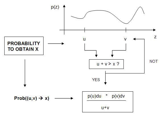
Figure 1: Derivation of the nonlinear evolution operator $T$ for the agent-based economic model given by Eqs. (1). See explanation in the text.

Now, we recall how to derive $T$ (see Ref. lopezruiz2011 ). Suppose that $p_{n}$ is the wealth distribution in the ensemble at time $n$. The probability that two agents with money $(u,v)$ interact will be $p_{n}(u)*p_{n}(v)$. As the trading is totally random, their exchange can give rise with equal probability to any value $x$ comprised in the interval $(0,u+v)$. Then, the probability to obtain a particular $x$ (with $x<u+v$) for the interacting pair $(u,v)$ will be $p_{n}(u)*p_{n}(v)/(u+v)$. Finally, we can obtain the probability to have money $x$ at time $n+1$. It will be the sum of the probabilities for all the pairs of agents $(u,v)$ able to generate the quantity $x$, that is, all the pairs verifying $u+v>x$. $T$ has then the form of a nonlinear integral operator (see Fig. 1),

$$p_{n+1}(x)={T}p_{n}(x)=\int\!\!\int_{u+v>x}\,{p_{n}(u)p_{n}(v)\over u+v}\;{\mathrm{d}}u{\mathrm{d}}v\,.$$ (4)

If we suppose $T$ acting in the PDFs space, we prove in the next section that $T$ conserves the mean wealth of the system, $<Tp>=<p>$. It also conserves the norm ($||\cdot||$), i.e. $T$ maintains the total number of agents of the system, $||Tp||=||p||=1$, that by extension implies the conservation of the total richness of the system. We also show that the exponential distribution $p_{f}(x)$ with the right average value is the only steady state of $T$, i.e. $Tp_{f}=p_{f}$, and that order two periodic points do not exist. It also seems feasible that other high period orbits do not exist. In consequence, it can be argued that the relation (3) is true. See for instance simulations done in Fig. 2. The same result is obtained for any other initial distribution shiva2011 .

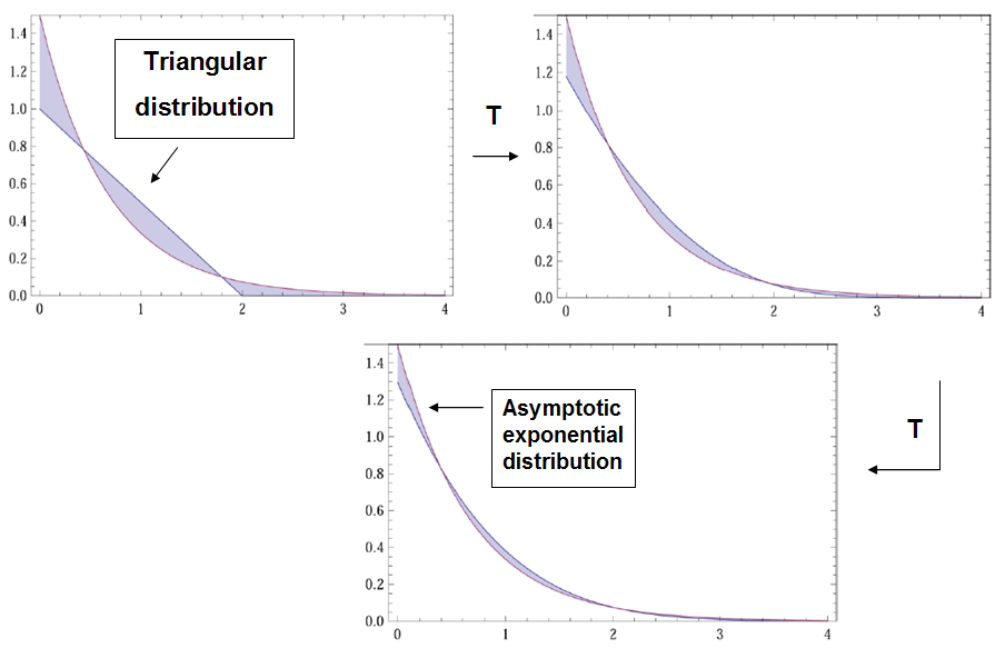
Figure 2: An example of the action of $T$ in the space of PDFs. In this case, $p_{0}(x)$ is chosen as a normalized triangular distribution. Observe that after two iterations of $T$ the system has practically reached the asymptotic state, i.e. the exponential distribution $p_{f}(x)$. (Figure avanced from shiva2011 ).

3 Properties of operator $T$

3.1 Definitions

Definition 1

We introduce the space $L_{1}^{+}$ of positive functions (wealth distributions) in the interval $[0,\infty)$,

$$L_{1}^{+}[0,\infty)=\{y:[0,\infty)\to R^{+}\cup\{0\},\hskip 5.69054pt||y||<\infty\},$$

with norm

$$||y||=\int_{0}^{\infty}y(x)dx.$$

Definition 2

We define the mean richness $<x>_{y}$ associated to a wealth distribution $y\in L_{1}^{+}[0,\infty)$ as the mean value of $x$ for the distribution $y$. In the rest of the paper, we will represent it by $<y>$. Then,

$$<y>\equiv<x>_{y}=||xy(x)||=\int_{0}^{\infty}xy(x)dx.$$

Definition 3

For $x\geq 0$ and $y\in L_{1}^{+}[0,\infty)$ the action of operator $T$ on $y$ is defined by

$$T(y(x))=\int\int_{S(x)}dudv{y(u)y(v)\over u+v},$$

with $S(x)$ the region of the plane representing the pairs of agents $(u,v)$ which can generate a richness $x$ after their trading, i.e.

$$S(x)=\{(u,v),\hskip 5.69054ptu,v>0,\hskip 5.69054ptu+v>x\}.$$

After some manipulations, other representations of the integral operator $T$ are possible:

$$(Ty)(x)={1\over 2}\int_{x}^{\infty}{dr\over r}\int_{-r}^{r}dt\,\,y\left({r+t\over 2}\right)y\left({r-t\over 2}\right),$$ (5)

$$(Ty)(x)=x\left[\int_{0}^{1}dt\int_{1-t}^{\infty}ds+\int_{1}^{\infty}dt\int_{0}^{\infty}ds\right]{y(xt)y(xs)\over t+s},$$

$$(Ty)(x)=x\left[\int_{0}^{\infty}dt\int_{0}^{\infty}ds-\int_{0}^{1}dt\int_{0}^{1-t}ds\right]{y(xt)y(xs)\over t+s},$$

$$(Ty)(x)=\int_{x}^{\infty}dr\int_{0}^{1}du\,\,y(ur)y((1-u)r).\hskip 85.35826pt$$

3.2 Theorems

Theorem 3.1

For any $y\in L_{1}^{+}[0,\infty)$ we have that $||Ty||=||y||^{2}$. In particular, for $y$ being a PDF, i.e. if $||y||=1$, then $||Ty||=1$. (It means that the number of agents in the economic system is conserved in time).

Proof

Take $y\in L_{1}^{+}[0,\infty)$. Then (see Fig. 3)

$$||Ty||=\int_{0}^{\infty}dx\int\int_{S(x)}dudv{y(u)y(v)\over u+v}=\hskip 39.83368pt$$

$$=\int_{0}^{\infty}du\int_{0}^{\infty}dv\int_{0}^{u+v}dx{y(u)y(v)\over u+v}=$$

$$=\int_{0}^{\infty}y(u)du\int_{0}^{\infty}y(v)dv=||y||^{2}.\hskip 14.22636pt\clubsuit$$

Corollary 1

It is clear that $(Ty)(x)>0$ for $x>0$ and $Ty\in L_{1}^{+}[0,\infty)$. Also, it is straightforward to see that $Ty$ is a continuous function, i.e. $Ty\in\mathbb{C}[0,\infty)$. Therefore, from the above Theorem we have that $Ty\in L_{1}^{+}[0,\infty)\bigcap\mathbb{C}[0,\infty)$, that is $T:L_{1}^{+}[0,\infty)\longrightarrow L_{1}^{+}[0,\infty)\bigcap\mathbb{C}[0,\infty)$.

Corollary 2

Consider the subset of PDFs in $L_{1}^{+}[0,\infty)$, i.e. the unit sphere $B:=\{y\in L_{1}^{+}[0,\infty)$, $||y||=1\}$. Observe that if $y\in B$ then $Ty\in B$. Therefore, we can define the restriction $T_{B}$ of $T$ to the subset $B$, that is $T_{B}:B\to B$.

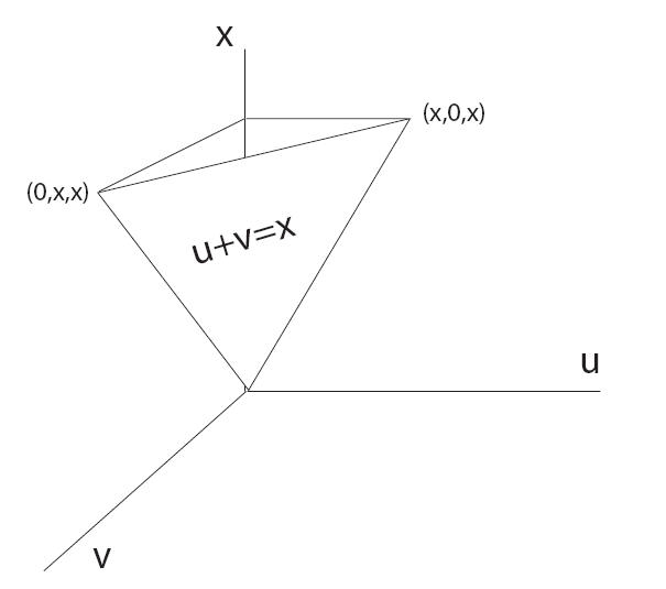
Figure 3: Integration region in the triple integral considered in the proof of Theorem 3.1.

Proposition 1

The operator $T$ is Lipchitz continuous in $B$ with Lipchitz constant $\leq 2$.

Proof

Take $y,w\in B$. Then

$$||Ty-Tw||=\hskip 170.71652pt$$

$$=\int_{0}^{\infty}du\int_{0}^{\infty}dv\int_{0}^{u+v}dx{|y(u)y(v)-w(u)w(v)|\over u+v}=\hskip 28.45274pt$$

$$=\int_{0}^{\infty}du\int_{0}^{\infty}dv|y(u)y(v)-y(u)w(v)+\hskip 56.9055pt$$

$$\hskip 28.45274pt+y(u)w(v)-w(u)w(v)|\leq\hskip 34.14322pt$$

$$\leq\int_{0}^{\infty}y(u)du\int_{0}^{\infty}dv|y(v)-w(v)|+\hskip 85.35826pt$$

$$+\int_{0}^{\infty}w(v)dv\int_{0}^{\infty}du|y(u)-w(u)|=2||y-w||.\hskip 14.22636pt\clubsuit$$

Theorem 3.2

The mean value $<y>$ of a PDF $y$ is conserved, that is $<Ty>=<y>$ for any $y\in B$. (It means that the mean wealth, and by extension the total richness, of the economic system are preserved in time).

Proof

$$<Ty>=||x(Ty)(x)||=\int_{0}^{\infty}xdx\int\int_{S(x)}dtds{y(t)y(s)\over t+s}=$$

$$=\int_{0}^{\infty}dt\int_{0}^{\infty}ds\int_{0}^{t+s}xdx{y(t)y(s)\over t+s}=$$

$$={1\over 2}\int_{0}^{\infty}dt\int_{0}^{\infty}ds(t+s)y(t)y(s)=$$

$$={1\over 2}\int_{0}^{\infty}ty(t)dt+{1\over 2}\int_{0}^{\infty}sy(s)ds=$$

$$=\int_{0}^{\infty}xy(x)dx=||xy(x)||=<y>.\hskip 14.22636pt\clubsuit$$

Observation: Because $||Ty||=||y||^{2}$ in $L_{1}^{+}[0,\infty)$, this operator divides the space $L_{1}^{+}[0,\infty)$ in three regions: the interior of the unit ball $B_{in}=\{y\in L_{1}^{+}[0,\infty)$, $||y||<1\}$, the unit sphere $B$ defined in Corollary 2, and the exterior of the unit ball $B_{ex}=\{y\in L_{1}^{+}[0,\infty)$, $||y||>1\}$. Accordingly, the recursion

$$y_{n}(x)=T^{n}y_{0}(x),\hskip 14.22636pt\hbox{with}\hskip 8.5359pty_{0}(x)\in L_{1}^{+}[0,\infty),$$

with the norm $||\cdot||$ has three different behaviors depending on $y_{0}$:

• If $y_{0}\in B_{in}$, then $\lim_{n\to\infty}||y_{n}(x)||=0$.

• If $y_{0}\in B$, then $||y_{n}(x)||=1$ (the succession $y_{n}$ remains in $B$ $\forall$ $n$).

• If $y_{0}\in B_{ex}$, then $\lim_{n\to\infty}||y_{n}(x)||=\infty$.

Then, it is obvious that $y=0$ is a fixed point of $T$. The remaining fixed points of $T$ in $L_{1}^{+}[0,\infty)$, if any, must be located in $B$. In fact, we have the following Theorem.

Theorem 3.3

Apart from $y=0$, the one-parameter family of functions $y_{\alpha}(x)=\alpha e^{-\alpha x}$, $\alpha>0$, are the unique fixed points of $T$ in the space $L_{1}^{+}[0,\infty)$.

Proof

They are fixed points. Using the representation (5) we find (see Figure 4) that

$$T\left(\alpha e^{-\alpha x}\right)={\alpha^{2}\over 2}\int_{x}^{\infty}dr\int_{-r}^{r}dt{e^{-\alpha r}\over r}=$$

$$\hskip 56.9055pt=\alpha^{2}\int_{x}^{\infty}e^{-\alpha r}dr=\alpha e^{-\alpha x}.$$

To see the uniqueness, consider the Fourier transform of $y\in L_{1}^{+}[0,\infty)$:

$$\bar{y}(p)=\int_{0}^{\infty}e^{ipx}y(x)dx,$$

and the Fourier transform of $Ty\in L_{1}^{+}[0,\infty)$:

$$(\overline{Ty})(p)=\int_{0}^{\infty}e^{ipx}dx\int\int_{S(x)}{dudv\over u+v}y(u)y(v)=$$

$$=\int_{0}^{\infty}duy(u)\int_{0}^{\infty}dvy(v)\int_{0}^{u+v}dx{e^{ipx}\over u+v}=$$

$$={1\over ip}\int_{0}^{\infty}duy(u)\int_{0}^{\infty}dvy(v){e^{ip(u+v)}-1\over u+v}.\hskip 8.5359pt$$

If $(Ty)(x)=y(x)$ then $(\overline{Ty})(p)=\bar{y}(p)$ and

$$ip\bar{y}(p)=\int_{0}^{\infty}duy(u)\int_{0}^{\infty}dvy(v){e^{ip(u+v)}-1\over u+v}.$$

Taking the derivative with respect to $p$ in both sides of this equality we find that the Fourier transform $\bar{y}(p)$ satisfies the differential equation:

$$\bar{y}(p)+p\bar{y}^{\prime}(p)=\bar{y}^{2}(p),$$

whose general solution is

$$\bar{y}(p)={1\over 1-cp},\hskip 28.45274ptc\in C.$$

When we are considering only positive functions $y(x)$, their Fourier transform must satisfy $\bar{y}(p)^{*}=\bar{y}(-p)$. This is only possible if $c=-c^{*}$, that is, the constant $c$ must be purely imaginary: $c=i/\alpha$, $\alpha\in R$ and then

$$\bar{y}(p)={1\over 1-(i/\alpha)p},\hskip 28.45274pt\alpha\in R.$$

From the inverse theorem for the Fourier transform [cham , p. 61, Theorem 8.3] we have that any solution $y(x)$ of the equation $Ty=y$ in $L_{1}^{+}[0,\infty)$ is of the form:

$$y(x)={1\over 2\pi}\lim_{\epsilon\to 0}\int_{-\infty}^{\infty}{e^{-ipx-\epsilon|p|}\over 1-(i/\alpha)p}dp.$$

From [wong , p. 197, Lemma 1] we have that

$$y(x)={1\over 2\pi}\int_{-\infty}^{\infty}{e^{-ipx}\over 1-(i/\alpha)p}dp.$$

Because $x>0$, the integrand is exponentially small when the imaginary part of $p$ is large and negative. Then, we can close the integration line $(-\infty,\infty)$ with a semi-infinite circle on the lower complex $p$-plane:

$$y(x)={1\over 2\pi}\int_{\cal C}{e^{-ipx}\over 1-(i/\alpha)p}dp,$$

where ${\cal C}$ is the union of the real line and that semicircle traveled in the negative sense (clockwise). The pole $p=-i\alpha$ of the integrand is outside of ${\cal C}$ if $\alpha<0$ and inside ${\cal C}$ if $\alpha>0$. Applying the Cauchy Residua Theorem to the above integral we obtain that

$$y(x)=\left\{\begin{array}[]{l}0\hskip 36.98866pt{\rm if}\hskip 5.69054pt\alpha<0,\\ \alpha e^{-\alpha x}\hskip 14.22636pt{\rm if}\hskip 5.69054pt\alpha>0.\end{array}\right.$$

Then, $y=0$ and $y_{\alpha}(x)=\alpha e^{-\alpha x}$, $\alpha>0$, are the unique fixed points of $T$ in the space $L_{1}^{+}[0,\infty)$. $\hskip 14.22636pt\clubsuit$

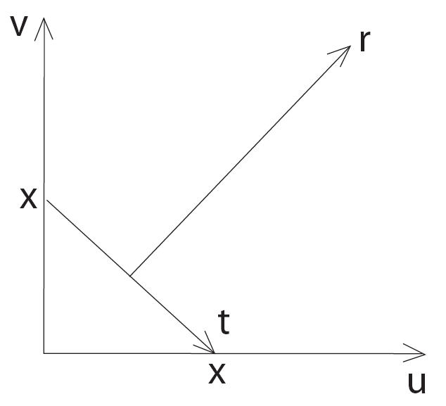
Figure 4: Integration region in the double integral considered in the proof of Theorem 3.3.

Corollary 3

The family of functions $y_{\alpha}(x)=\alpha e^{-\alpha x}$, $\alpha>0$, are the unique fixed points of $T_{B}$ (the restriction of $T$ in the unit ball $B$).

As we will show with some examples in the next section, the numerical results indicate that, apart from the family of exponential distributions, there is no other periodic or aperiodic asymptotic sets for the operator $T$ acting on the PDFs ball $B$. Thus, the whole unit ball $B$ seems to contract to the exponential steady-state regime. In the next Theorem, we make another step in this direction by showing that the operator $T$ has no cycles of order two.

Theorem 3.4

The operator $T$ has not cycles of order two in $L_{1}^{+}[0,\infty)$, that is, $T^{2}y=y\Rightarrow Ty=y$.

Proof

A similar computation to the one introduced in the proof of Theorem 3.3 shows that

$$\left\{\begin{array}[]{lll}(\overline{Ty})(p)&=\displaystyle{\int_{0}^{\infty}duy(u)\int_{0}^{\infty}dvy(v){e^{ip(u+v)}-1\over ip(u+v)},}\\ (\overline{T^{2}y})(p)&=\displaystyle{\int_{0}^{\infty}du(Ty)(u)\int_{0}^{\infty}dv(Ty)(v){e^{ip(u+v)}-1\over ip(u+v)}}=\\ &=\overline{y}(p).\end{array}\right.$$

Taking the derivative with respect to $p$ in both sides of both equations, we obtain the following system of differential equations for $\overline{y}(p)$ and $(\overline{Ty})(p)$:

$$\left\{\begin{array}[]{cc}[p(\overline{Ty})(p)]^{\prime}=&\overline{y}^{2}(p),\\ \,[p\overline{y}(p)]^{\prime}=&(\overline{Ty})^{2}(p).\end{array}\right.$$

Taking the cross product of these equations and multiplying by $p^{2}$ we get the equation:

$$p^{2}\overline{y}^{2}(p)[p\overline{y}(p)]^{\prime}=p^{2}(\overline{Ty})^{2}(p)[p(\overline{Ty})(p)]^{\prime}\,,$$

and integrating:

$$(\overline{Ty})^{3}(p)=\overline{y}^{3}(p)+{c\over p^{3}}\,,\hskip 28.45274ptc\in\mathbb{C}.$$

But both, $\overline{y}(p)$, $(\overline{Ty})(p)\in{\cal C}(-\infty,\infty)$ and then $c=0$. This means $(\overline{Ty})(p)=\overline{y}(p)$ and $(Ty)(x)=y(x)$ (a.e.). $\hskip 14.22636pt\clubsuit$

To finish this section, another interesting property of operator $T$ concerning to the value of the norm of the derivatives of $T^{n}y$ is disclosed in the following Proposition. A consequence of this property is also given.

Proposition 2

For any $y\in L_{1}^{+}[0,\infty)$ and $m,n\in N$, with $m\leq n$, we have the following properties:

$$(T^{n}y)\hskip 5.69046pt\hbox{is $m$ times differentiable},$$

$$(-1)^{m}(T^{n}y)^{(m)}\in L_{1}^{+}[0,\infty),$$

$$||(T^{n}y)^{(m)}||=|(T^{n}y)^{(m-1)}(0)|,$$

$$(-1)^{m}(T^{n}y)^{(m)}(0)=\hskip 113.81102pt$$

$$\hskip 51.21504pt={1\over m}\sum_{k=0}^{m-1}(T^{n-1}y)^{(k)}(0)(T^{n-1}y)^{(m-k-1)}(0).$$

Proof

For fixed $n$, let us show that $(T^{n}y)$ is $m$ times continuously differentiable and $(-1)^{m}(T^{n}y)^{(m)}\in L_{1}^{+}[0,\infty)$ by induction over $m$. It is obvious for $m=0$: $(T^{n}y)$ is continuous and $(T^{n}y)\in L_{1}^{+}[0,\infty)$ for any $n=1,2,3,\ldots$ Suppose that it is true for a certain $m-1<n$ and let us show that it is also true for $m$. From the last representation of the integral operator $T$ given after Definition 3, we have that

$$(T^{n}y)^{\prime}(x)=-\int_{0}^{1}(T^{n-1}y)(ux)(T^{n-1}y)((1-u)x)du<0,$$

and then

$$(-1)^{m}(T^{n}y)^{(m)}(x)=\hskip 170.71652pt$$

$$\sum_{k=0}^{m-1}\dbinom{m-1}{k}\int_{0}^{1}u^{k}(1-u)^{m-k-1}\left[(-1)^{k}(T^{n-1}y)^{(k)}(ux)\right]$$

$$\hskip 48.36958pt\times\left[(-1)^{m-k-1}(T^{n-1}y)^{(m-k-1)}((1-u)x)\right]du.$$

From the induction hypothesis, all the integrands in the above sum of integrals are continuous and then $(T^{n}y)^{(m)}$ is continuous and integrable. Moreover, they are positive and then $(-1)^{m}(T^{n}y)^{(m)}(x)>0$. The last two assertions of the Proposition are trivial. $\hskip 14.22636pt\clubsuit$

As a consequence of the former Proposition, we have:

Proposition 3

A fixed point $y$ of $T$, if any, must be a completely monotonic function: $y\in{\cal C}^{\infty}[0,\infty)$ and $(-1)^{m}y^{(m)}(x)\geq 0$ $\forall x\in[0,\infty)$. Then, as it can be easily tested, the exponential distribution $y_{\alpha}(x)=\alpha e^{-\alpha x}$, $\alpha>0$, is one of such type of functions.

Proof

If $Ty=y$ for a certain $y\in L_{1}^{+}[0,\infty)$, then $T^{n}y=y$ for any $n\in N$. For arbitrary $m\in N$, take $n\geq m$. Our goal is proved just seeing from the former Proposition that $(-1)^{m}y^{(m)}(x)=(-1)^{m}(T^{n}y)^{(m)}(x)\geq 0$. $\hskip 14.22636pt\clubsuit$

4 Time evolution of $T$: Examples

As discussed in the former section, the iteration of $T$ for any PDF $y$ in the unit ball $B$ with a finite $<y>$ seems to converge toward the only fixed point of the system, i.e. the exponential distribution presenting the same mean value of the initial condition $y$. In this respect, we make the following conjecture:

Conjecture For any $y\in B$ with a finite $<y>$,

$$\lim_{n\to\infty}(T^{n}y)(x)=\alpha e^{-\alpha x}$$

with

$${1\over\alpha}=<y>=\int_{0}^{\infty}xy(x)dx.$$

From simulations (see Fig. 2), it can be guessed that the convergence suggested in this conjecture is fast. Next, we compute and verify the contraction of the dynamics toward the exponential distribution under the action of $T$ for some particular PDFs.

Example 1

For $\alpha>0$ and $n\in\mathbb{N}$, consider the family

$$y_{\alpha,n}(x)={\alpha^{n+1}\over n!}x^{n}e^{-\alpha x}\in B.$$

The mean value is:

$$<y_{\alpha,n}>=\gamma^{-1}=(n+1)/\alpha.$$

The limit distribution of $T^{n}y_{\alpha,n}$ when $n\to\infty$ should be $w(x)=\gamma e^{-\gamma x}$. The first iteration is:

$$(Ty_{\alpha,n})(x)={\alpha\sqrt{\pi}\over 2^{2n+1}n!\Gamma(n+3/2)}\Gamma(2n+1,\alpha x).$$

We numerically check that

$$||Ty_{\alpha,n}-w||<||y_{\alpha,n}-w||$$

for different values of $\alpha$ and $n$.

Example 2

For $\alpha$, $\beta>0$, consider the new family

$$y_{\alpha,\beta}(x)={1\over 2}\left[\alpha e^{-\alpha x}+\beta e^{-\beta x}\right]\in B.$$

The mean value is:

$$<y_{\alpha,\beta}>=\gamma^{-1}={\alpha\beta\over 2(\alpha+\beta)}.$$

The limit distribution should be $w(x)=\gamma e^{-\gamma x}$. The first iteration of $T$ gives

$$(Ty_{\alpha,\beta})(x)=\hskip 170.71652pt$$

$$={1\over 4}\left\{\alpha e^{-\alpha x}+\beta e^{-\beta x}+{2\alpha\beta\over\alpha-\beta}\left[\Gamma(0,\beta x)-\Gamma(0,\alpha x)\right]\right\}.$$

Again, we numerically check that

$$||Ty_{\alpha,\beta}-w||<||y_{\alpha,\beta}-w||.$$

for several values of $\alpha$ and $\beta$.

Example 3

For $\alpha>0$ and $n\in\mathbb{N}$, consider the $\epsilon$-family of functions

$$y_{\epsilon,\alpha,n}(x)=(1-\epsilon)\alpha e^{-\alpha x}+\epsilon{\alpha^{n+1}\over n!}x^{n}e^{-\alpha x}$$

with $0\leq\epsilon\leq 1$. It is straightforward to see that $y_{\epsilon,\alpha,n}\in B$. The mean value is:

$$<y_{\epsilon,\alpha,n}>=\gamma^{-1}={1+\epsilon n\over\alpha}.$$

The limit function should be $w(x)=\gamma e^{-\gamma x}$. The first iteration is:

$$Ty_{\epsilon,\alpha,n}(x)=\alpha\left\{1+\epsilon\left[\epsilon-2+{2(1-\epsilon)\over(n+1)!}e^{\alpha x}\Gamma(n+1,\alpha x)+\right.\right.$$

$$\hskip 56.9055pt\left.\left.+{\epsilon\sqrt{\pi}\over 4^{n}n!}{e^{\alpha x}\over 2\Gamma(n+3/2)}\Gamma(2n+1,\alpha x)\right]\right\}e^{-\alpha x}.$$

Numerically, it is found that

$$||Ty_{\epsilon,\alpha,n}-w||<||y_{\epsilon,\alpha,n}-w||$$

for different values of $\epsilon$, $n$ and $\alpha$.

5 Conclusions

From a macroscopic point of view, markets have an intrinsic random ingredient as a consequence of the interaction of an undetermined set of agents at each moment. Also the unknowledge of the exact quantities of money exchanged by the agents at each moment contributes to the randomness of the global system. Even under these circumstances, the system can reach an equilibrium. Concretely, it has been found in western societies that the exponential distribution fits well the wealth distribution for the income of the $95\%$ of the population.

A statistical model recently introduced lopezruiz2011 that takes into account all these idealistic random characteristics has been considered in this work. Some of its mathematical properties have been carefully worked out and presented here. These exact results help us to understand why the exponential distribution is computationally found as the asymptotic steady state of this continuous economic model. This fact certifies that markets, as well as many other similar statistical systems ranging from physics to biology, can be modeled as dissipative dynamical systems having the exponential distribution, or any other distribution if it is the case, as a stable equilibrium, particularly under totally random conditions.

References

- (1) A. Dragulescu, V.M. Yakovenko, Physica A 299, 213 (2001)
- (2) V.M. Yakovenko, in Encyclopedia of Complexity and System Science, Meyers, R.A. (Ed.) (Springer, Germany, 2009)
- (3) B.K. Chakrabarti, A. Chatterjee, A. Chakraborti, S. Sinha, Econophysics: An Introduction (Willey-VCH Verlag GmbH, Germany, 2010)
- (4) A. Dragulescu, V.M. Yakovenko, Eur. Phys. J. B 17, 723 (2000)
- (5) J. Gonzalez-Estevez, M.G. Cosenza, R. Lopez-Ruiz, J.R. Sanchez, Physica A 387, 4637 (2008)
- (6) C. Pellicer-Lostao, R. Lopez-Ruiz, Int. J. Mod. Phys. C 22, 21 (2011)
- (7) A. Chatterjee, B. K. Chakraborti, S. S. Manna, Physica A 335, 155 (2004)
- (8) R. Lopez-Ruiz, J.L. Lopez, X. Calbet, ESAIM: Proceedings of the ECIT-2010 Conference (Setember 2010), to appear (2011)
- (9) X. Calbet, J.L. Lopez, R. Lopez-Ruiz, Physical Review E 83, 036108 (2011)
- (10) R. Lopez-Ruiz, E. Shivanian, S. Abbasbandy, J.L. Lopez, arXiv:1104.2187 (2011)
- (11) D.C. Champeney, A Handbook of Fourier Theorems, (Cambridge Univ. Press, New York, 1987)
- (12) R. Wong, Asymptotic Approximations of Integrals, (Academic Press, New York, 1989)