Initial value representation for the $\mathrm{SU}(n)$ semiclassical propagator

Abstract

The semiclassical propagator in the representation of $\mathrm{SU}(n)$ coherent states is characterized by isolated classical trajectories subjected to boundary conditions in a doubled phase space. In this paper we recast this expression in terms of an integral over a set of initial-valued trajectories. These trajectories are monitored by a filter that collects only the appropriate contributions to the semiclassical approximation. This framework is suitable for the study of bosonic dynamics in $n$ modes with fixed total number of particles. We exemplify the method for a Bose-Einstein condensate trapped in a triple-well potential, providing a detailed discussion on the accuracy and efficiency of the procedure.

I Introduction

Semiclassical methods have proved to be very useful in the investigation of systems with many degrees of freedom, especially in atomic and molecular dynamicsMiller (2001); Thoss and Wang (2004); Kay (2005); Miller (2006). Moreover, the semiclassical approximation has also been an important theoretical tool in studying the connection between the classical and quantum theories, particularly in fundamental topics such as chaos and open quantum systemsKoch et al. (2008); Moix and Pollak (2008); Goletz, Koch, and Großmann (2010).

The semiclassical propagator in the coordinate representation was first derived by Van VleckVan Vleck (1928) at the beginning of the last century. However, this fundamental result has two remarkable characteristics that considerably hinder its practical application. First, the Van Vleck propagator is determined by classical trajectories subject to boundary conditions. In general, the search for these specific solutions is quite complicated, particularly in multidimensional and chaotic systems. The second major problem is the appearance of focal points, which are responsible for divergences in the semiclassical approximation.

A different line of research, concerned with the difficulties caused by focal points, led to the development of semiclassical propagators in the representation of the harmonic-oscillator coherent statesKlauder and Skagerstam (1985); Baranger et al. (2001); Martín-Fierro and Llorente (2007); Braun and Garg (2007). Although it has been found that the focal points still persisted, this alternative approach has demonstrated some evident advantages over the coordinate and momentum representations, including an immediate visualization of the system over the full phase space. Nevertheless, new problems have emerged, such as the duplication of the phase space, resulting from the apparent overdetermination of the classical equations of motion. Furthermore, not all classical trajectories in the extended phase space, while correctly satisfying the boundary conditions, correspond to semiclassical propagators with physical meaningHuber and Heller (1987); Huber, Heller, and Littlejohn (1988); Adachi (1989); Rubin and Klauder (1995); Shudo and Ikeda (1995, 1996); Ribeiro, de Aguiar, and Baranger (2004); de Aguiar et al. (2005). Therefore, it is necessary to establish effective rules for selecting the proper contributions to the semiclassical dynamics.

In the last decades, many different techniques have been proposed in order to solve the recurrent problems in semiclassical propagationMiller (1970, 1974); Heller (1975); Herman and Kluk (1984); Kay (1994a, b, 1997); Zhang and Pollak (2003, 2004); Heller (1991); Tomsovic and Heller (1991); Shalashilin and Child (2004); Shalashilin and Burghardt (2008); Pollak and Shao (2003); Kay (2006). Most of these methods are based on the concept of initial value representation, in which the system dynamics is determined only by initial conditions, avoiding the search for boundary-valued trajectories.

Recently, Aguiar et al. presented a new approach to the semiclassical propagator of the harmonic-oscillator coherent states, which combines the unique resources offered by the trajectories in a doubled phase space with the plain advantages of an initial value representationde Aguiar, Vitiello, and Grigolo (2010). Moreover, they demonstrated that practical and simple rules for selecting the contributing trajectories can produce very accurate results.

The procedures developed in the present paper are similar to those of Aguiar et al., but generalized to a subclass of the $\mathrm{SU}(n)$ coherent states. These states constitute an ideal setting to study the bosonic dynamics for a fixed total number of particles in $n$ modes. In this paper we also propose a new prescription for the selection of contributing trajectories, which we designate as a heuristic filter. For a detailed derivation of the $\mathrm{SU}(n)$ semiclassical propagator we refer the reader to a recent work of the present authorsViscondi and de Aguiar .

The remainder of the paper is organized as follows: in section II we develop the semiclassical propagation method based on an initial value representation. We start with a brief review of the $\mathrm{SU}(n)$ coherent states, in which we introduce fundamental aspects of the adopted notation. Then, we present the $\mathrm{SU}(n)$ semiclassical propagator, followed by other important definitions, such as the effective classical Hamiltonian, the classical equations of motion and the doubled phase space. Next we reformulate the semiclassical approximation in terms of a set of initial conditions and a heuristic filter of trajectories. At the end of the section, we describe the procedure used for calculating semiclassical mean values of observables, based on the phase space representation of states. Section III presents an application of the $\mathrm{SU}(2)$ and $\mathrm{SU}(3)$ semiclassical propagators. As an example, we consider a simplified model for the dynamics of a Bose-Einstein condensate in a triple-well potential. In this context, we introduce the classical approximation, which provides a reference for comparison with the semiclassical results. Also, we discuss the accuracy of the semiclassical propagation in nonlinear and predominantly linear dynamical regimes, by contrasting the approximations with exact quantum calculations. Finally, in section IV we present our concluding remarks.

II Semiclassical propagation method for $\mathrm{SU}(n)$

II.1 $\mathrm{SU}(n)$ coherent states

The coherent state related to the fully symmetric irreducible representation of $\mathrm{SU}(n)$ for $N$ identical bosons is given byGilmore, Bowden, and Narducci (1975):

$$|w\rangle=\sum\limits_{m_{1}+m_{2}+\ldots+m_{n}=N}\left(\frac{N!}{m_{1}!m_{2}!\ldots m_{n}!}\right)^{\frac{1}{2}}\left(\prod\limits_{j=1}^{n-1}w_{j}^{m_{j}}\right)\frac{|m_{1},m_{2},\ldots,m_{n}\rangle}{(1+w^{*}w)^{\frac{N}{2}}};$$ (1)

where $\{|m_{1},m_{2},\ldots,m_{n}\rangle\}$ is the usual basis of the bosonic Fock space $\mathds{B}^{n}_{N}$ for $n$ modes and $N$ particles, such that $m_{j}$ is the occupation in the $j$-th mode. The vector $w=(w_{1},w_{2},\ldots,w_{n-1})^{T}$, with $(n-1)$ complex entries, parametrizes the entire set of coherent states.

Although normalized, the coherent states in (1) are not orthogonal:

$$\langle w^{\prime}|w\rangle=\frac{(1+w^{\prime*}w)^{N}}{(1+w^{\prime*}w^{\prime})^{\frac{N}{2}}(1+w^{*}w)^{\frac{N}{2}}}.$$ (2)

However, due to the overcompleteness of the coherent states, we can write the following diagonal resolution for the identity in $\mathds{B}_{N}^{n}$:

$$\int\limits_{w\,\in\,\mathds{C}^{n-1}}d\mu(w^{*},w)\;|w\rangle\langle w|=\mathds{1};\qquad d\mu(w^{*},w)=\frac{\sigma(n)\,\mathrm{dim}(\mathbb{B}_{N}^{n})}{(1+w^{*}w)^{n}}\prod\limits_{j=1}^{n-1}d^{2}w_{j};$$ (3)

where $d^{2}w_{j}=dx_{j}dy_{j}$, with $x_{j}=\mathrm{Re}\left(w_{j}\right)$ and $y_{j}=\mathrm{Im}\left(w_{j}\right)$. Note that the normalization factor in (3) can be divided into $\sigma(n)=\frac{(n-1)!}{\pi^{n-1}}$, which is independent of the total boson number, and $\mathrm{dim}(\mathbb{B}_{N}^{n})=\frac{(N+n-1)!}{N!(n-1)!}$, the dimension of the accessible Hilbert space.

II.2 $\mathrm{SU}(n)$ semiclassical propagator

The quantum propagator in the $\mathrm{SU}(n)$ coherent state representation is defined as the transition probability between the initial coherent state $|w_{i}\rangle$ and final coherent state $|w_{f}\rangle$ after a time interval $\tau$:

$$K(w^{*}_{f},w_{i};\tau)=\langle w_{f}|e^{-iH\tau}|w_{i}\rangle.$$ (4)

After recasting the above propagator as a path integral, we can perform its semiclassical approximation, which consists in expanding the action functional to second order around a classical trajectory. The result of this derivationViscondi and de Aguiar is given by:

$$K_{sc}(w^{*}_{f},w_{i};\tau)=e^{i(S+I)-\frac{N}{2}\mathrm{Ln}\left[(1+|w^{*}_{f}|^{2})(1+|w_{i}|^{2})\right]}\sqrt{\left[\frac{1+\overline{w}(\tau)w(\tau)}{1+\overline{w}(0)w(0)}\right]^{\frac{n}{2}}\det\left[\frac{\partial\overline{w}(0)}{\partial\overline{w}(\tau)}\right]}.$$ (5)

All elements of this semiclassical formula are calculated on a classical trajectory, which is solution of the equations of motion

$$\left\{\begin{aligned} \dot{w}&=-\frac{i}{N}(1+\overline{w}w)\left[\mathds{1}+w\otimes\overline{w}\right]\frac{\partial\mathcal{H}}{\partial\overline{w}}=-i\xi\frac{\partial\mathcal{H}}{\partial\overline{w}}\\ \dot{\overline{w}}&=\frac{i}{N}(1+\overline{w}w)\left[\mathds{1}+\overline{w}\otimes w\right]\frac{\partial\mathcal{H}}{\partial w}=i\overline{\xi}\frac{\partial\mathcal{H}}{\partial w}\end{aligned}\right.$$ (6)

with boundary conditions

$$w(0) =w_{i};$$ (7)

$$\overline{w}(\tau) =w^{*}_{f}.$$

In equation (6), $\mathcal{H}$ is the effective classical Hamiltonian:

$$\mathcal{H}(\overline{w},w)=\frac{\langle\overline{w}^{*}|H|w\rangle}{\langle\overline{w}^{*}|w\rangle}.$$ (8)

If the classical equations of motion have more than one solution subject to the same boundary conditions $w_{i}$ and $w_{f}^{*}$ with fixed time interval $\tau$, then the correct semiclassical propagator between these points is given by the sum of the propagators (5) for each possible trajectory.

Note that the complex vector variables $w$ and $\overline{w}$ are completely independent, i.e. in general $\overline{w}(t)\neq w^{*}(t)$. This doubled phase space is a direct consequence of the introduction of boundary conditions to the equations of motion. If $\overline{w}(t)$ were equal to $w^{*}(t)$, the two vector differential equations in (6) would be redundant and the boundary conditions $w(0)=w_{i}$ and $w^{*}(\tau)=w^{*}_{f}$ would make the problem overdetermined. Therefore, the duplication of the phase space is required to solve the classical equations of motion in the coherent state representation.

The equations of motion (6) are derived by the extremization of the following action functional:

$$S(w^{*}_{f},w_{i};\tau)=\int\limits_{0}^{\tau}L\left(\overline{w},w,\dot{\overline{w}},\dot{w}\right)dt+\Gamma(w^{*}_{f},w_{i};\tau);$$ (9)

$$L\left(\overline{w},w,\dot{\overline{w}},\dot{w}\right)=i\frac{N}{2}\frac{\overline{w}\dot{w}-\dot{\overline{w}}w}{1+\overline{w}w}-\mathcal{H}(\overline{w},w);$$

$$\Gamma(w^{*}_{f},w_{i};\tau)=-i\frac{N}{2}\mathrm{Ln}\left\{[1+w^{*}_{f}w(\tau)][1+\overline{w}(0)w_{i}]\right\}.$$

The function $\Gamma$, known as the boundary term, is essential in obtaining the classical equation of motion subject to the boundary conditions (7). Another quantity introduced in (5) is the correction term to the action:

$$I=\frac{1}{4}\int\limits_{0}^{\tau}\mathrm{Tr}\left[\frac{\partial}{\partial\overline{w}}\left(\overline{\xi}\frac{\partial\mathcal{H}}{\partial w}\right)+\frac{\partial}{\partial w}\left(\xi\frac{\partial\mathcal{H}}{\partial\overline{w}}\right)\right]dt$$ (10)

where the matrices $\xi$ and $\overline{\xi}$ are defined in equations (6).

The last ingredient required in the formula (5) is the tangent matrix $\mathbb{M}$, governing the dynamics of small displacements around the classical trajectory, defined in block form by

$$\left(\begin{array}[]{c}\delta w(\tau)\\ \delta\overline{w}(\tau)\end{array}\right)=\left(\begin{array}[]{c c}M_{11}(\tau)&M_{12}(\tau)\\ M_{21}(\tau)&M_{22}(\tau)\end{array}\right)\left(\begin{array}[]{c}\delta w(0)\\ \delta\overline{w}(0)\end{array}\right)=\mathbb{M}\left(\begin{array}[]{c}\delta w(0)\\ \delta\overline{w}(0)\end{array}\right).$$ (11)

Notice that

$$M_{22}(\tau)=\frac{\partial\overline{w}(\tau)}{\partial\overline{w}(0)}=\left[\frac{\partial\overline{w}(0)}{\partial\overline{w}(\tau)}\right]^{-1}$$ (12)

and,therefore, the block $M_{22}$ is the inverse of the matrix whose determinant appears in the semiclassical propagator. A focal point in the variables $\overline{w}$ corresponds to a zero value of $\det M_{22}(\tau)$ and, consequently, to a divergence in (5).

The tangent matrix can be calculated as solution of a system of differential equations subjected to initial conditions. Using (6), we obtain

$$\left(\begin{array}[]{c}\delta\dot{w}\\ \delta\dot{\overline{w}}\end{array}\right)=\left(\begin{array}[]{c c}-i\frac{\partial}{\partial w}\left[\xi\frac{\partial\mathcal{H}}{\partial\overline{w}}\right]&-i\frac{\partial}{\partial\overline{w}}\left[\xi\frac{\partial\mathcal{H}}{\partial\overline{w}}\right]\\ i\frac{\partial}{\partial w}\left[\,\overline{\xi}\frac{\partial\mathcal{H}}{\partial w}\right]&i\frac{\partial}{\partial\overline{w}}\left[\,\overline{\xi}\frac{\partial\mathcal{H}}{\partial w}\right]\end{array}\right)\left(\begin{array}[]{c}\delta w\\ \delta\overline{w}\end{array}\right)=\mathbb{R}\left(\begin{array}[]{c}\delta w\\ \delta\overline{w}\end{array}\right).$$ (13)

Substituting the definition (11) in (13), we find

$$\dot{\mathbb{M}}(t)=\mathbb{R}(t)\mathbb{M}(t).$$ (14)

with initial conditions

$$\mathbb{M}(0)=\mathds{1}.$$ (15)

However, note that the matrix $\mathbb{R}(t)$ is calculated on the classical trajectory, which in its turn is subject to boundary conditions. Also notice that the differential equations (14) couple the blocks of the tangent matrix exclusively in pairs. Therefore, we need to consider only the equations of motion for $M_{12}(t)$ and $M_{22}(t)$, with initial conditions $M_{12}(0)=0$ and $M_{22}(t)=\mathds{1}$.

II.3 Initial value representation

The classical trajectory is the fundamental quantity for calculating all elements of the semiclassical propagator. However, finding the classical solution represents a boundary condition problem, whose analytical or numerical resolution generally exhibits greater technical difficulties or higher computational cost than a similar problem subject to initial conditions. Therefore, the development of semiclassical propagation methods based on initial conditions, known as initial value representations, is highly desirable. In this section we develop such a method for (5).

First, we use the resolution of the identity (3) to reconstruct a specific propagator from an integral over the entire set of propagators with the same initial coherent state:

$$K(w^{*}_{f},w_{i};\tau) =\langle w_{f}|e^{-iH\tau}|w_{i}\rangle$$ (16)

$$=\int\limits_{\overline{w}(\tau)\,\in\,\mathds{C}^{n-1}}d\mu(\overline{w}^{*}(\tau),\overline{w}(\tau))\;\langle w_{f}|\overline{w}^{*}(\tau)\rangle\langle\overline{w}^{*}(\tau)|e^{-iH\tau}|w_{i}\rangle$$

$$=\int\limits_{\overline{w}(\tau)\,\in\,\mathds{C}^{n-1}}d\mu(\overline{w}^{*}(\tau),\overline{w}(\tau))\;\langle w_{f}|\overline{w}^{*}(\tau)\rangle K(\overline{w}(\tau),w_{i};\tau)$$

Next we consider $\overline{w}(\tau)$ as a function of the initial values of its corresponding trajectory:

$$\overline{w}(\tau)=\overline{w}(\overline{w}_{i},w_{i};\tau);$$ (17)

where $\overline{w}_{i}=\overline{w}(0)$. Thus, the integrand in the last line of (16) also becomes a function of $\overline{w}_{i}$ implicitly in $\overline{w}(\tau)$. The change of integration variables introduces the following Jacobian determinant:

$$\prod\limits_{j=1}^{n-1}d^{2}\overline{w}_{j}(\tau)=\left|\det\left[\frac{\partial\overline{w}(\tau)}{\partial\overline{w}(0)}\right]\right|^{2}\prod\limits_{j=1}^{n-1}d^{2}\overline{w}_{j}(0)=\left|\det M_{22}(\tau)\right|^{2}\prod\limits_{j=1}^{n-1}d^{2}\overline{w}_{j}(0).$$ (18)

We should note that the mapping between $\overline{w}_{i}$ and $\overline{w}(\tau)$ is not injective, due to the existence of focal points. However, the determinant of $M_{22}$ is zero at these problematic values of $\overline{w}(\tau)$, so that their contribution to the integral is null.

Finally, considering the semiclassical approximation for the propagators in the integrand and substituting the expression (18) in (16), we obtain the first form for the semiclassical propagator in the initial value representation:

$$K_{sc}^{ivr}(w^{*}_{f},w_{i};\tau)=\int\limits_{\overline{w}_{i}\,\in\,\mathds{C}^{n-1}}d^{2}\overline{w}_{i}\,\frac{\sigma(n)\,\mathrm{dim}(\mathbb{B}_{N}^{n})\left|\det M_{22}(\tau)\right|^{2}}{(1+\overline{w}^{*}(\tau)\overline{w}(\tau))^{n}}\langle w_{f}|\overline{w}^{*}(\tau)\rangle K_{sc}(\overline{w}(\tau),w_{i};\tau);$$ (19)

where $d^{2}\overline{w}_{i}=\prod\limits_{j=1}^{n-1}d^{2}\overline{w}_{j}(0)$. Notice that the integrand of (19) is now proportional to $\left|\det M_{22}(\tau)\right|^{\frac{3}{2}}$, instead of the inconvenient factor $\left|\det M_{22}(\tau)\right|^{-\frac{1}{2}}$ in equation (5). Thus we avoid the potential divergences of the semiclassical propagator corresponding to focal points in the variables $\overline{w}$. Also note that all quantities in the integrand of (19) are calculated on the trajectory with initial conditions $w(0)=w_{i}$ and $\overline{w}(0)=\overline{w}_{i}$. Therefore, by calculating the semiclassical propagator $K_{sc}(\overline{w}(\overline{w}_{i},w_{i};\tau),w_{i},\tau)$ for a grid of initial conditions with $w_{i}$ fixed, we obtain the semiclassical propagator $K_{sc}^{ivr}(w^{*}_{f},w_{i};\tau)$, at the desired arrival point, after an integration in $\overline{w}_{i}$.

However, our scheme to recast the propagator in terms of initial conditions seems to have some disadvantages in relation to the original boundary condition problem. At first glance, we replaced the calculation of a single propagator by an infinite number of propagators, which are calculated for all possible values of $\overline{w}_{i}$. Even though the latter are subjected to initial conditions, the large number of propagators in the integration can make this method impracticable. But experience tells us that the trajectories with major contribution to the integral (19) are associated with values of $\overline{w}_{i}$ close to $w_{i}^{*}$. Therefore, the integral (19) is usually calculated for a small grid around $w_{i}^{*}$, considerably reducing the number of classical trajectories required in a practical application.

The second problem in the expression (19) is the need to carry out a new integration for each choice of the final coherent state, parametrized by $w_{f}$. However, all dependence on $w_{f}$ in the integrand of (19) comes from the factor $\langle w_{f}|\overline{w}^{*}(\tau)\rangle$. Hence, using the identity (2), we can perform a multinomial expansion in the numerator of the coherent state overlap, thus extracting $w_{f}$ from the integration sign:

$$K_{sc}^{ivr}(w^{*}_{f},w_{i};\tau)=\sum\limits_{m_{1}+\ldots+m_{n}=N}\frac{N!}{m_{1}!\ldots m_{n}!}\frac{1}{(1+w^{*}_{f}w_{f})^{\frac{N}{2}}}\left[\prod\limits_{j=1}^{n-1}(w^{*}_{f,j})^{m_{j}}\right]\mathcal{I}_{m_{1},\ldots,m_{n}}$$ (20)

Hence, in order to calculate the semiclassical propagator for an arbitrary final coherent state, we need to perform only $\mathrm{dim}(\mathbb{B}_{N}^{n})$ integrations whose values are independent of $w_{f}$:

$$\mathcal{I}_{m_{1},\ldots,m_{n}}(w_{i};\tau) =\int d^{2}\overline{w}_{i}\,\frac{\sigma(n)\,\mathrm{dim}(\mathbb{B}_{N}^{n})\left|\det M_{22}(\tau)\right|^{2}\prod\limits_{j=1}^{n-1}\left[\overline{w}^{*}_{j}(\tau)\right]^{m_{j}}}{(1+\overline{w}^{*}(\tau)\overline{w}(\tau))^{\frac{N}{2}+n}}K_{sc}(\overline{w}(\tau),w_{i};\tau)$$ (21)

$$=\left(\frac{N!}{m_{1}!m_{2}!\ldots m_{n}!}\right)^{-\frac{1}{2}}\left.\langle m_{1},m_{2},\ldots,m_{n}|e^{-iH\tau}|w_{i}\rangle\right|_{sc}.$$

The second equality shows that the integrals $\mathcal{I}_{m_{1},\ldots,m_{n}}$ can be rewritten as semiclassical propagators between the initial coherent state and a number state, except by a combinatorial factor.

II.4 Heuristic filters

It is well known that some trajectories in the doubled phase space give unphysical contributions to the semiclassical propagatorAdachi (1989); Rubin and Klauder (1995); Shudo and Ikeda (1995, 1996); de Aguiar et al. (2005); de Aguiar, Vitiello, and Grigolo (2010). Therefore, given a grid of initial conditions $\overline{w}_{i}$, only part of the resulting classical trajectories participate in the calculation of the integrals (21). The appropriate contributions can be collected using the heuristic filter defined by:

$$\frac{d}{dt}\mathrm{Ln}\left(\left|K_{sc}(\overline{w}(t),w_{i};t)\right|^{2}\right)<\lambda.$$ (22)

The classical trajectories that violate this condition at time $t$ are discarded from the integration for $\tau>t$. Note that the only free parameter in the initial value representation is $\lambda$, whose positive value should be adjusted in order to optimize the semiclassical propagation.

The idea behind this filter is the following: if we write the semiclassical propagator as $K_{sc}=e^{\alpha+i\beta}$, with $\alpha,\beta\in\mathds{R}$, then the inequality (22) can be recast in the form $\frac{d\alpha}{dt}<\frac{\lambda}{2}$. Therefore, the discarded trajectories are those that lead to an abrupt positive change in the real part of $\mathrm{Ln}\left(K_{sc}\right)$, thus causing the divergence of the absolute value of the propagator. As seen in the equation (5), the time variations in $\alpha$ are directly determined by the imaginary part of the corrected action $(S+I)$. However, unlike previously published methodsRubin and Klauder (1995); de Aguiar, Vitiello, and Grigolo (2010), the proposed heuristic filter also takes into account the factor that contains the determinant of the tangent matrix. Clearly, the modulus of this factor also affects the value of $\alpha$, either counteracting abrupt negative changes in $\mathrm{Im}(S+I)$ or contributing to the divergence of the semiclassical propagator. The inclusion of this aspect in the heuristic filter is an important element in the present work, which greatly improved the results in section III.

II.5 $Q$ representation with $\mathrm{SU}(n)$ coherent states

Using the expressions (20) and (21), we can easily calculate the semiclassical propagator at any point $w$ of the classical phase space, for fixed initial condition $w_{i}$ and period of propagation $\tau$. Thus, we obtain a complete description of the system state, known as the Husimi or $Q$ representationScully and Zubairy (1997). In general, the function $Q(w^{*},w)$ associated with an arbitrary state $|\psi\rangle$ is defined as:

$$Q(w^{*},w) =\langle w|\rho|w\rangle$$ (23)

$$=|K(w^{*},w_{i};\tau)|^{2};$$

where $\rho=|\psi\rangle\langle\psi|$ is the density operator for a pure state and $|w\rangle$ is given by equation (1). In the second line of (23) we assume that $|\psi\rangle=e^{-iH\tau}|w_{i}\rangle$. Therefore, using the $\mathrm{SU}(n)$ semiclassical propagator, we can directly construct the semiclassical representation $Q_{sc}(w^{*},w)=|K_{sc}(w^{*},w_{i},\tau)|^{2}$.

With the aid of the expression (3) and assuming $\langle\psi|\psi\rangle=1$ we find that:

$$\int\limits_{w\,\in\,\mathds{C}^{n-1}}d\mu(w^{*},w)\;Q(w^{*},w)=1.$$ (24)

Unlike the exact definition (4), the semiclassical propagators (5) and (20) do not preserve the norm of the state during its evolutionde Aguiar, Vitiello, and Grigolo (2010). Therefore, for a proper comparison with the quantum results at time $\tau$, we need to normalize $Q_{sc}$ according to the relation (24). The normalization of the quantum and semiclassical representations is implied in the remainder of the paper.

In terms of the exact $Q$ function or of its semiclassical version $Q_{sc}$, we can readily obtain the mean of an arbitrary observable $O$:

$$\langle O\rangle=\int d\mu(w^{*},w)\mathcal{O}_{\mathrm{a}}(w^{*},w)Q(w^{*},w).$$ (25)

The function $\mathcal{O}_{\mathrm{a}}$, which corresponds to the antinormally ordered symbol of the operator $O$, is defined by

$$O=\int d\mu(w^{*},w)\mathcal{O}_{\mathrm{a}}(w^{*},w)|w\rangle\langle w|.$$ (26)

III Application and discussion of the semiclassical propagator

III.1 Bose-Einstein condensate in a triple-well trapping potential

In order to illustrate the method described in previous sections, we discuss here its application to $\mathrm{SU}(2)$ and $\mathrm{SU}(3)$ coherent states, considering a simplified model for the dynamics of a Bose-Einstein condensate in a triple-well potentialViscondi and Furuya . Assuming that the three wells of the trap are identical and equivalently coupled, the Hamiltonian of the model in a three-mode approximation is given by:

$$H=\Omega\sum\limits_{j\neq k}a^{{\dagger}}_{j}a_{k}+\frac{\chi}{(N-1)}\sum\limits_{j=1}^{3}(a^{{\dagger}}_{j})^{2}a_{j}^{2};$$ (27)

where $a_{j}$ ($a^{{\dagger}}_{j}$) is the bosonic annihilation (creation) operator related to the single-particle state $|u_{j}\rangle$, which represents the ground state of a harmonic oscillator centered on $j$-th minimum of the trapping potential, for $j=1,2,3$. The parameters $\Omega$ and $\chi$ correspond to the rates of tunneling and collision of trapped bosons, respectively.

Note that $H$ preserves the total number of particles, so that we can restrict our analysis to invariant subspaces with fixed $N$, denoted by $\mathds{B}^{3}_{N}$. Therefore, the $\mathrm{SU}(3)$ coherent states, defined in equation (1) with $n=3$, are appropriate to study the model. Substituting (27) in (8), we obtain the effective classical Hamiltonian:

$$\frac{\mathcal{H}}{N}= \Omega\frac{\overline{w}_{1}w_{2}+\overline{w}_{2}w_{1}+\overline{w}_{1}+w_{1}+\overline{w}_{2}+w_{2}}{1+\overline{w}_{1}w_{1}+\overline{w}_{2}w_{2}}$$ (28)

$$+\chi\frac{\overline{w}_{1}^{2}w_{1}^{2}+\overline{w}_{2}^{2}w_{2}^{2}+1}{(1+\overline{w}_{1}w_{1}+\overline{w}_{2}w_{2})^{2}}.$$

Then, employing the general formula (6), we find the classical equations of motion for the condensate:

$$i\dot{w}_{j} =\Omega(1+w_{1}+w_{2})(1-w_{j})+2\chi\frac{w_{j}(\overline{w}_{j}w_{j}-1)}{1+\overline{w}_{1}w_{1}+\overline{w}_{2}w_{2}}$$ (29)

$$-i\dot{\overline{w}}_{j} =\Omega(1+\overline{w}_{1}+\overline{w}_{2})(1-\overline{w}_{j})+2\chi\frac{\overline{w}_{j}(\overline{w}_{j}w_{j}-1)}{1+\overline{w}_{1}w_{1}+\overline{w}_{2}w_{2}}$$

for $j=1,2$. Using (28) and (29), we can easily obtain the other dynamical quantities relevant to the calculation of the semiclassical propagator, such as the Lagrangian $L$ and the matrix $\mathbb{R}$. According to the equations (29), the dynamics of the condensate exhibits three classical invariant subspaces, described by the following conditions:

$$w_{1}=w_{2},\;\overline{w}_{1}=\overline{w}_{2}$$ (30a)

$$w_{1}=1,\;\overline{w}_{1}=1$$ (30b)

$$w_{2}=1,\;\overline{w}_{2}=1$$ (30c)

For simplicity, we limit our discussion to the case (30a), since the three invariant subspaces are dynamically equivalentViscondi and Furuya . Now, we show that the effective quantum dynamics of the condensate under the constraints (30) can be approximated by $\mathrm{SU}(2)$ semiclassical propagators. For this purpose, we rewrite the coherent state (1) in terms of bosonic creation operators:

$$|w\rangle=\frac{1}{\sqrt{N!}}\left[\begin{array}[]{c}\displaystyle{\frac{\sum\limits_{j=1}^{n-1}w_{j}a^{{\dagger}}_{j}+a^{{\dagger}}_{n}}{(1+w^{*}w)^{\frac{1}{2}}}}\end{array}\right]^{N}|0\rangle.$$ (31)

Then, we apply the condition (30a) to the equation (31) for $n=3$:

$$|w_{1},w_{2}=w_{1}\rangle_{{}_{SU(3)}} =\frac{1}{\sqrt{N!}}\left[\frac{w_{1}(a^{{\dagger}}_{1}+a^{{\dagger}}_{2})+a^{{\dagger}}_{3}}{(1+2w^{*}_{1}w_{1})^{\frac{1}{2}}}\right]^{N}|0\rangle$$ (32)

$$=\frac{1}{\sqrt{N!}}\left[\frac{\sqrt{2}w_{1}b^{{\dagger}}_{1}+b^{{\dagger}}_{2}}{(1+2w^{*}_{1}w_{1})^{\frac{1}{2}}}\right]^{N}|0\rangle$$

$$=|\sqrt{2}w_{1}\rangle_{{}_{SU(2)}};$$

where we performed a change of basis in the single-particle Hilbert space, corresponding to the following unitary transformation of the bosonic creation operatorsNegele and Orland (1998):

$$\left\{\begin{aligned} b^{{\dagger}}_{1}&=\frac{1}{\sqrt{2}}\left(a^{{\dagger}}_{1}+a^{{\dagger}}_{2}\right)\\ b^{{\dagger}}_{2}&=a^{{\dagger}}_{3}\\ b^{{\dagger}}_{3}&=\frac{1}{\sqrt{2}}\left(a^{{\dagger}}_{1}-a^{{\dagger}}_{2}\right)\end{aligned}\right.$$ (33)

According to the equation (32), when restricted to a invariant subspace under the classical dynamics, the $\mathrm{SU}(3)$ coherent states are reduced to the $\mathrm{SU}(2)$ coherent states with parameter $\sqrt{2}w_{1}$.

Also notice that the state presented in (32) has zero occupation number in the mode associated with the operator $b^{{\dagger}}_{3}$. Therefore, the constraint (30a) is classically equivalent to the equation $\langle b^{{\dagger}}_{3}b_{3}\rangle=0$. However, by applying the transformation (33) to the Hamiltonian (27), we can easily see that the mean occupation $\langle b^{{\dagger}}_{3}b_{3}\rangle$ does not remain zero under the quantum evolution of the condensate, considering any state initially unoccupied in this mode. Consequently, the subspaces (30) do not have quantum counterparts with identical characteristics. However, we can still use the $\mathrm{SU}(2)$ coherent states to approximate the semiclassical dynamics under these restrictions. This approximation should provide accurate results when a similar evolution in the unrestricted space displays irrelevant values of $\langle b^{{\dagger}}_{3}b_{3}\rangle$.

III.2 Classical approximation

In order to establish a criterion for comparison between the semiclassical and quantum results, we now introduce a third approach to the bosonic dynamics, which we call classical approximation.

We designate as principal trajectory, indicated by the subindex ‘$p$’, the solution of the classical equations of motion (6) subject to initial conditions $w_{p}(0)=w_{i}$ and $\overline{w}_{p}(0)=w^{*}_{i}$. In this case the two vector equations in (6) become redundant, since the solution is such that $w_{p}(t)=\overline{w}^{*}_{p}(t)$.

The classical approximation to the mean of an arbitrary observable $O$ at the time $\tau$ is defined as follows:

$$\langle O\rangle_{c}(\tau) =\langle w_{p}(\tau)|O|w_{p}(\tau)\rangle;$$ (34)

where $|w_{p}(\tau)\rangle$ indicates the coherent state parametrized by the principal trajectory $w_{p}(\tau)$. The classical approximation consists simply in calculating the function $\mathcal{O}_{\mathrm{n}}(w^{*},w)=\langle w|O|w\rangle$, which represents the normally ordered symbol of the operator $O$, on the principal trajectory.

Assuming an initial state $|w_{i}\rangle_{{}_{\mathrm{SU}(n)}}$, the classical approximation of $\langle O\rangle(t)$ is exact in only two specific situations when compared with the corresponding quantum results: (i) for $H\in\mathrm{su}(n)$, because in this case $|w_{p}(\tau)\rangle$ differs from the correct solution of the Schr dinger equation by no more than a global phaseZhang, Feng, and Gilmore (1990); (ii) in the macroscopic limit, given by $N\rightarrow\infty$Yaffe (1982).

Clearly, the semiclassical approximation is more accurate than the classical approach (34), since it adds quantum corrections to the classical results. Therefore, the semiclassical propagator (5) is also exact for any linear Hamiltonian in the generators of $\mathrm{SU}(n)$ ($H\in\mathrm{su}(n)$) as well as in the macroscopic limit ($N\rightarrow\infty$).

Under the restriction $H\in\mathrm{su}(n)$, every initial condition $\overline{w}_{i}$ must provide a trajectory with appropriate contribution to the integral (21). Accordingly, the heuristic filter (22) must allow the contribution of all trajectories at all instants of time, which it does, because $\left|K_{sc}(\overline{w}(t),w_{i};t)\right|^{2}$ is constant with respect to $t$ for linear Hamiltonians.

It follows that the classical and semiclassical approximations to the Hamiltonian (27) are exact for $\chi=0$, since in this regime $H$ is linear in the generators of $\mathrm{SU}(3)$ (bilinear in the creation and annihilation operators). Therefore, the bosonic collisions introduce nonlinear terms to the condensate dynamics, whose classical and semiclassical descriptions are not complete for a finite number of particles. Consequently, we expect the application of the semiclassical propagator (20) to be better behaved for weak nonlinearities (small values of $\chi$) and large numbers of bosons.

III.3 Semiclassical approximation with $\mathrm{SU}(2)$ coherent states

A relevant observable in the condensate dynamics is the population imbalance operator $S_{z}$, which describes the difference in occupation between the two effectively occupied modes in the classical invariant subspace (30a):

$$S_{z}=\frac{b^{{\dagger}}_{1}b_{1}-b^{{\dagger}}_{2}b_{2}}{2}$$ (35)

Figure 1 compares the semiclassical, quantum and classical evolution of $\langle S_{z}\rangle/S$ for $N=30$, $\Omega=-1$ and $\chi=-1$, considering as initial state $|\sqrt{2}w_{1}\rangle_{{}_{\mathrm{SU}(2)}}=|\tan\frac{\pi}{8}\rangle_{{}_{\mathrm{SU}(2)}}$. The mean of $S_{z}$ is normalized by the quantity $S=\frac{N}{2}$ so that $-1\leq\langle S_{z}\rangle/S\leq 1$. For the semiclassical approximation we used the $\mathrm{SU}(2)$ propagator with $479$ initial conditions $\overline{w}_{i}$ and limiting value $\lambda=10$ for the heuristic filter.

Figure 1: Classical (dashed green), quantum (dotted red) and semiclassical (solid blue) evolution of the normalized mean of the population imbalance operator $S_{z}$ for the initial state $|\sqrt{2}w_{1}\rangle_{{}_{\mathrm{SU}(2)}}=|\tan\frac{\pi}{8}\rangle_{{}_{\mathrm{SU}(2)}}$. The parameters of the Hamiltonian assume the values $N=2S=30$, $\Omega=-1$ and $\chi=-1$. The $\mathrm{SU}(2)$ semiclassical propagation was performed with a grid of $479$ initial conditions and limiting filter $\lambda=10$.

Notice that the oscillations of the classical mean display constant amplitude, unlike the semiclassical and quantum results. Although restricted to the $\mathrm{SU}(2)$ propagator, the semiclassical method shows quantitative agreement with the exact quantum calculations, being fairly superior to the classical approximation, even for a relatively small number of particles. In general, the classical and semiclassical approximations are accurate for sufficiently short times, but the quality of the semiclassical evolution is obviously higher for longer periods of propagation, when the nonlinear terms of the quantum Hamiltonian become important.

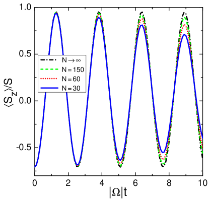
Figure 2: Semiclassical evolution of $\langle S_{z}\rangle/S$ for $N=30$ (solid blue), $N=60$ (dotted red) and $N=150$ (dashed green). The dash-dotted black curve represents the classical approximation, which is equivalent to the macroscopic limit $N\rightarrow\infty$. In all results we consider $\Omega=-1$, $\chi=-1$ and initial state $|\sqrt{2}w_{1}\rangle_{{}_{\mathrm{SU}(2)}}=|\tan\frac{\pi}{8}\rangle_{{}_{\mathrm{SU}(2)}}$.

Figure 2 shows the behavior of the semiclassical evolution of $\langle S_{z}\rangle/S$ with the variation of the total number of particles, for $\Omega=-1$, $\chi=-1$ and initial state $|\sqrt{2}w_{1}\rangle_{{}_{\mathrm{SU}(2)}}=|\tan\frac{\pi}{8}\rangle_{{}_{\mathrm{SU}(2)}}$. The results correspond to the $\mathrm{SU}(2)$ semiclassical propagator for $30$, $60$ and $150$ particles, with $\lambda=10$ and about $500$ initial conditions in each case.

Note that the equations of motion (29) and their solutions, including the principal trajectory $w_{p}(t)$, are independent of the total number of particles. Therefore, it is easy to show that, for a linear operator in the generators of $\mathrm{SU}(3)$, the classical mean per particle is also independent of $N$. Therefore, quantities like $\langle S_{z}\rangle_{c}/S$ represent the macroscopic limit of their quantum and semiclassical counterparts, since the classical approximation (34) is exact for $N\rightarrow\infty$.

In accordance with the previous discussion, we included the classical approximation in figure 2 as the macroscopic limit for the dynamics of the semiclassical means. Note that the semiclassical results quickly converge to the classical curve with increasing $N$. Consequently, we expect the classical approximation to show high accuracy for a few hundred condensate bosons, which represents a scenario compatible with usual experiments. However, the semiclassical propagators must provide superior results for the mesoscopic dynamics when subjected to longer periods of propagation or more intense nonlinear effects.

Figure 3: Diagram of contributing trajectories for the $\mathrm{SU}(2)$ semiclassical propagator with $N=30$, $\Omega=-1$, $\chi=-1$ and initial state $|\sqrt{2}w_{1}\rangle_{{}_{\mathrm{SU}(2)}}=|\tan\frac{\pi}{8}\rangle_{{}_{\mathrm{SU}(2)}}$. Each initial condition $\overline{w}_{i}$ is represented by a square whose color indicates the period of contribution of the corresponding trajectory, according to the heuristic filter (22) for $\lambda=10$.

Figure 3 shows the diagram of contributing trajectories for the $\mathrm{SU}(2)$ semiclassical propagator with $N=30$, $\Omega=-1$, $\chi=-1$ and initial state $|\sqrt{2}w_{1}\rangle_{{}_{\mathrm{SU}(2)}}=|\tan\frac{\pi}{8}\rangle_{{}_{\mathrm{SU}(2)}}$. This diagram corresponds to the semiclassical approximation shown in figure 1 and reproduced in figure 2. Each square in figure 3 represents an initial condition $\overline{w}_{i}$ used in the numerical calculation of the integrals (21). The color code indicates the time of contribution of the resulting classical trajectories, determined by the heuristic filter (22) with $\lambda=10$.

Notice that the trajectories with the most significant contributions have initial conditions $\overline{w}_{i}$ centered around $w_{i}^{*}=\frac{1}{\sqrt{2}}\tan\frac{\pi}{8}\approx 0.29$. This initial value defines the principal trajectory, whose contribution is among the most important in the reconstruction of the semiclassical propagator. Note also that $w^{*}_{i}$ is the value that maximizes the $Q$ representation for the state $|\sqrt{2}w^{*}_{i}\rangle_{{}_{\mathrm{SU}(2)}}$. Therefore, this coherent state is located in the same region of phase space responsible for the most relevant contributions to the initial value representation.

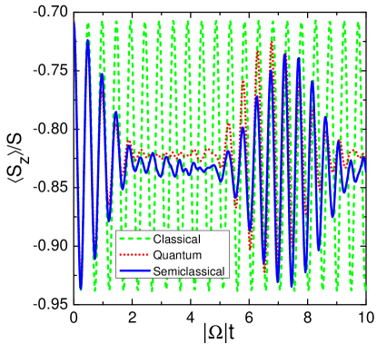
Figure 4: Classical (dashed green), quantum (dotted red) and semiclassical (solid blue) evolution of $\langle S_{z}\rangle/S$ for $N=30$, $\Omega=-1$, $\chi=-8$ and coherent initial state $|\sqrt{2}w_{1}\rangle_{{}_{\mathrm{SU}(2)}}=|\tan\frac{\pi}{8}\rangle_{{}_{\mathrm{SU}(2)}}$. The semiclassical approximation was performed with the $\mathrm{SU}(2)$ propagator, considering a grid of $3781$ initial conditions and $\lambda=18$.

In general, the equations of motion resulting from the Hamiltonian (27) show significant changes in behavior for different magnitudes of the ratio $\chi/\Omega$Viscondi, Furuya, and de Oliveira (2010); Viscondi and Furuya , which represents the relative intensity between the quadratic and linear terms of $H$. The previous examples of application of the semiclassical propagator are restricted to small absolute values of $\chi/\Omega$, since the linear terms are clearly dominant in the dynamics of the condensate. Figure 4 displays the semiclassical, quantum and classical dynamics of $\langle S_{z}\rangle/S$ in a strongly nonlinear regime, for $N=30$, $\Omega=-1$, $\chi=-8$ and initial state $|\sqrt{2}w_{1}\rangle_{{}_{\mathrm{SU}(2)}}=|\tan\frac{\pi}{8}\rangle_{{}_{\mathrm{SU}(2)}}$. In the semiclassical approximation, we employed the $\mathrm{SU}(2)$ propagator for a grid of $3781$ initial conditions and limiting value $\lambda=18$.

Again we see that the amplitude of the classical mean remains constant during the whole evolution of the system. Conversely, the semiclassical and quantum results exhibit an almost complete ‘collapse’ of the oscillations, followed by a partial ‘revival’ of the amplitude value in relation to the classical approximation. Therefore, this example refers to a strongly nonlinear and exclusively quantum behavior, described with excellent accuracy by the semiclassical propagator. However, note that the number of trajectories required for a proper semiclassical approximation is considerably larger than in the predominantly linear dynamics shown in figure 1. As expected, the semiclassical propagator loses computational efficiency in nonlinear regimes.

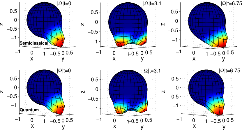
Figure 5: At the top (bottom) we show the $Q$ representation on the unit sphere related to the semiclassical (quantum) evolution of condensate at three different times, for $N=30$, $\Omega=-1$, $\chi=-8$ and initial state $|\sqrt{2}w_{1}\rangle_{{}_{\mathrm{SU}(2)}}=|\tan\frac{\pi}{8}\rangle_{{}_{\mathrm{SU}(2)}}$.

The phase space corresponding to the $\mathrm{SU}(2)$ coherent states may be identified as a spherical surfaceArecchi et al. (1972). It follows that, applying the definition (23) with the coherent states given by (32) under the transformation of variables $\sqrt{2}w_{1}=e^{-i\phi}\tan\frac{\theta}{2}$, we obtain the $Q$ representation for $\mathrm{SU}(2)$ in terms of angular spherical coordinates. In this way, we can represent an arbitrary quantum state on the unit sphere:

$$\left\{\ \begin{aligned} &x=[Q(\theta,\phi)+1]\sin\theta\cos\phi\\ &y=[Q(\theta,\phi)+1]\sin\theta\sin\phi\\ &z=-[Q(\theta,\phi)+1]\cos\theta\end{aligned}\right.$$ (36)

where $\phi\in[0,2\pi)$ and $\theta=[0,\pi]$. Notice that our definition for the variable $\theta$ has its origin in the negative $z$ semi-axis.

In figure 5 we show the comparison between the semiclassical (top) and quantum (bottom) $Q$ representations at three different times, for $N=30$, $\Omega=-1$, $\chi=-8$ and initial state $|\sqrt{2}w_{1}\rangle_{{}_{\mathrm{SU}(2)}}=|\tan\frac{\pi}{8}\rangle_{{}_{\mathrm{SU}(2)}}$. The represented states are in correspondence with the results displayed in figure 4.

At $|\Omega|t=0$ we show the initial coherent state, whose representation is identical in the semiclassical and quantum approaches. At the time $|\Omega|t=3.1$, we have the superposition of two localized states in phase space (‘Schr dinger-cat’ state), which is responsible for the oscillation collapse in $\langle S_{z}\rangle/S$. At $|\Omega|t=6.75$, we see that the $Q$ function converges again to a single location on the sphere. This behavior is associated with the revival of the oscillations in figure 4.

The differences between the quantum and semiclassical representations in figure 5 are almost imperceptible, evidencing that the semiclassical approximation accurately describes the delocalization and the subsequent relocalization of the state in the phase space.

III.4 $\mathrm{SU}(3)$ semiclassical propagator

Although the approximations with the $\mathrm{SU}(2)$ semiclassical propagator have shown excellent accuracy, the $\mathrm{SU}(3)$ coherent states are more appropriate to the dynamics determined by the Hamiltonian (27). Figure 6 exemplifies the use of the $\mathrm{SU}(3)$ semiclassical propagator in the evolution of $\langle S_{z}\rangle/S$, for $N=30$ $\Omega=-1$, $\chi=-1$ and initial coherent state parametrized by $w_{1}=w_{2}=\frac{1}{\sqrt{2}}\tan\frac{\pi}{8}$. In the calculation of the initial value representation we used $35134$ classical trajectories, whose contributions were determined by the heuristic filter (22) with $\lambda=10$. In comparison with the result for the $\mathrm{SU}(3)$ propagator, we reproduce in figure 6 the corresponding $\mathrm{SU}(2)$ approximation and the exact quantum evolution, also shown in figure 1.

As expected, the $\mathrm{SU}(3)$ semiclassical propagator is more accurate than the $\mathrm{SU}(2)$ approximation. The difference between these results comes mainly from the occupation of the mode associated with the operator $b^{{\dagger}}_{3}$. During the considered period of propagation, the normalized mean $\langle b^{{\dagger}}_{3}b_{3}\rangle/N$ grows monotonically until it reaches a value close to $0.04$ at $|\Omega|t=6$.

We conclude that most of the inaccuracy attributed to the $\mathrm{SU}(2)$ semiclassical propagator in figures 1 and 6 is due to the classical constraint (30a), since the $\mathrm{SU}(3)$ semiclassical approximation is almost exact in the predominantly linear dynamical regime.

Figure 6: Time evolution of $\langle S_{z}\rangle/S$ resulting from the $\mathrm{SU}(2)$ semiclassical propagator (dashed green), the $\mathrm{SU}(3)$ semiclassical propagator (solid blue) and the exact quantum calculation (dotted red), for $N=30$, $\Omega=-1$, $\chi=-1$ and initial coherent state parametrized by $w_{1}=w_{2}=\frac{1}{\sqrt{2}}\tan\frac{\pi}{8}$. In the $\mathrm{SU}(3)$ semiclassical approximation we used $35134$ classical trajectories, with contributing period determined by $\lambda=10$. The $\mathrm{SU}(2)$ semiclassical curve is the same one shown in figure 1.

IV Conclusion

We constructed an initial value representation for the $\mathrm{SU}(n)$ semiclassical propagator, which replaces the search for boundary-valued trajectories by an integral over a set of initial-valued trajectories in the doubled phase space. This formulation represents a considerable advantage in the calculation of the propagator, since the numerical or analytical resolution of a boundary condition problem is typically much more difficult than its initial condition counterpart, particularly in systems with many degrees of freedom. Moreover, our method allows the factorization of the arrival point $w^{*}_{f}$, as given in equation (20), considerably reducing the number of integrations required for a complete representation of the system.

The semiclassical approach showed excellent accuracy when compared to exact quantum results, even for a relatively small number of particles. The efficacy of the semiclassical approximation is largely due to the effective heuristic filter, which was able to discriminate the trajectories with appropriate contributions to the propagator. The systematic elimination of non-contributing trajectories represents a crucial component in the implementation of an initial value representation in the doubled phase space, because it directly determines the speed, precision and applicability of the method.

We tested our semiclassical formula for a triple-well Bose-Einstein condensate in nonlinear and predominantly linear dynamical regimes. Although the semiclassical propagation has been very satisfactory in both situations, the number of initial conditions required for an appropriate description of the nonlinear dynamics is significantly higher than in the almost linear case. In general, the computational efficiency of the semiclassical propagator is only limited by the required number of contributing classical trajectories. Clearly, this number grows with a exponent proportional to $(n-1)$, the dimension of the subspace $\overline{w}$. However, we can assume that the required number of initial conditions $\overline{w}_{i}$ decreases with the total number of particles, since the semiclassical results converge with increasing $N$ to the classical approximation, which is determined by a single trajectory. Therefore, the $\mathrm{SU}(n)$ semiclassical propagator is a viable alternative in the study of bosonic systems with many degrees of freedom and large number of particles, since the computational cost of exact quantum methods typically grows as a polynomial in $N$ of order proportional to $n$.

Finally, we would like to point out that the formulas (20) and (21), the main results of this paper, can be easily extended to other classes of coherent states, such as the usual harmonic-oscillator coherent states. Thus, this work also represents an alternative to previously published semiclassical methods.