Axial anomalies of Lifshitz fermions

LMU-ASC 07/11,    MPP-2011-35,    CERN-PH-TH/2011-051

Abstract

We compute the axial anomaly of a Lifshitz fermion theory with anisotropic scaling $z=3$ which is minimally coupled to geometry in $3+1$ space–time dimensions. We find that the result is identical to the relativistic case using path integral methods. An independent verification is provided by showing with spectral methods that the $\eta$–invariant of the Dirac and Lifshitz fermion operators in three dimensions are equal. Thus, by the integrated form of the anomaly, the index of the Dirac operator still accounts for the possible breakdown of chiral symmetry in non–relativistic theories of gravity. We apply this framework to the recently constructed gravitational instanton backgrounds of Hořava–Lifshitz theory and find that the index is non–zero provided that the space–time foliation admits leaves with harmonic spinors. Using Hitchin’s construction of harmonic spinors on Berger spheres, we obtain explicit results for the index of the fermion operator on all such gravitational instanton backgrounds with $SU(2)\times U(1)$ isometry. In contrast to the instantons of Einstein gravity, chiral symmetry breaking becomes possible in the unimodular phase of Hořava–Lifshitz theory arising at $\lambda=1/3$ provided that the volume of space is bounded from below by the ratio of the Ricci to Cotton tensor couplings raised to the third power. Some other aspects of the anomalies in non–relativistic quantum field theories are also discussed.

1 Introduction

Since the discovery of the axial anomaly and its profound success in explaining the two–photon decay mode of the $\pi^{0}$ meson [1, 2], there has been a lot of activity in the study of anomalous symmetries in quantum field theory and their geometrical and topological origin (see, for instance, [3] for a recent brief overview of the subject and its history) as well as in model building. The axial anomaly is accounted perturbatively by the one–loop fermion contribution (triangle diagram) of the two–photon coupling to an axial current, as in spinor electrodynamics, but it also has an alternative description in terms of the non–invariance of the Euclidean path integral measure under chiral rotations of the fermions coupled to a background gauge field [5] (see also the textbook [6]). This framework was soon afterwards generalized to fermions coupled to a background metric by computing the gravitational corrections to the axial anomaly associated to the two–graviton decay mode of the $\pi^{0}$ meson [7, 8, 9], which also enjoys a path integral derivation [5, 6] as for the case of gauge fields (see also [10] for the structure of gravitational anomalies in general dimensions). These results refer to the so called local form of the anomaly.

Another important development is related to the integrated form of axial anomaly which can be non–zero when the background gauge field is non–Abelian and topologically non–trivial. In this case, the four–dimensional Dirac operator exhibits normalizable zero modes with unequal number of positive and negative chirality solutions (denoted by $n_{\pm}$ respectively) in the background of an instanton configuration. Thus, there is chiral symmetry breaking induced by instantons that may in turn lead to baryon and lepton number violation in Yang–Mills theories [11]. This novel possibility is a physical manifestation of the Atiyah–Singer index theorem [12] (but see also the textbooks [13, 14]) that equates the index of the four–dimensional Dirac operator, namely $n_{+}-n_{-}$, to the topological charge $k$ of the background gauge field on the compactified Euclidean space-time $S^{4}$. (In the actual instanton solutions one has $n_{+}=k>0$ and $n_{-}=0$, whereas for the anti–instantons the situation is reversed, i.e., $n_{-}=-k>0$ and $n_{+}=0$.)

Likewise, the integrated form of the gravitational correction to the axial anomaly is a topological invariant given by (one eighth of) the Hirzebruch signature of space-time, which can be non-zero on topologically non–trivial gravitational backgrounds and may lead to similar results for chiral symmetry breaking by the index theorem of Dirac operator. This is certainly true for the Dirac operator on $K3$, which is the unique compact self–dual gravitational instanton without boundaries [15, 16]; in this case there are two covariantly constant negative helicity modes and no positive helicity modes so that $n_{+}-n_{-}=-2$. However, gravitational instantons with boundaries do not admit any normalizable zero modes of the Dirac operator, provided that the Ricci scalar curvature of space–time is non–negative (as it is by Einstein’s field equations when the cosmological constant is non–negative), and by a general result based on Lichnerowicz’s theorem [17] the index of Dirac operator vanishes on such backgrounds [18]. An alternative derivation of the same result is based on the Atiyah–Patodi–Singer index theorem [19, 20, 13] taking into proper account the boundary terms of space–time from the asymptotic regions [21, 22, 23, 24, 25, 26, 27, 28]. Thus, although the signature of space–time is non–zero, the index of the Dirac operator turns out to be zero for all gravitational instanton backgrounds with boundaries, in which case there is no chiral symmetry breaking induced by quantum tunneling effects. For a systematic exposition of all these matters we refer the interested reader to the report [29]. More explanations will also be given in the text.

In this paper we examine the chiral anomaly for non–relativistic fermions of Lifshitz type that are coupled to background fields in four space-time dimensions. Our investigation was prompted by the current activity on non-relativistic theories of gravity with anisotropic scaling, serving as alternatives to the ultraviolet completion of Einstein theory of gravitation with higher order spatial derivative terms [30, 31]. The resulting theory sacrifices relativistic invariance for perturbative renormalizability at short distances and despite criticism related to the presence of an unphysical mode and the difficulty to flow to ordinary gravity at large distances (see, for instance, [32, 33] and references therein, as well as [34]), it provides an interesting framework that should be given the benefit of the doubt to play a useful role in quantum gravity (see also [35] for a more recent proposal that defies some of the criticism). Coupling the theory to Lifshitz fermions with the same anisotropic scaling in space and time, as for gravity, is a step that we take in this work and which, apparently, has not been considered in the literature so far. The computations we present in the following provide the gravitational contribution to the axial anomaly at a Lifshitz point and, as such, they generalize rather naturally the results on the axial anomaly for Lifshitz fermions coupled to gauge field backgrounds [36]. In either case, the local form of the anomaly turns out to be identical to the relativistic case. These results are surprising at first sight, but clearly they should be related to the topological character of the anomaly that is proportional to the characteristic classes ${\rm Tr}(F\wedge F)$ and ${\rm Tr}(R\wedge R)$ for gauge and metric fields, respectively. They are also quite general since they treat the gauge and metric fields as background without reference to their field equations. As such, they provide the local form of the axial anomaly at a Lifshitz point and they are independent of the particular form of the bosonic action. This can make them useful for applications in other fields of current research that incorporate ideas of quantum criticality.

The integrated form of the axial anomaly at a Lifshitz point is also identical to the relativistic case, and, therefore, it equals the index of the relativistic Dirac operator in a given background. This will be shown explicitly by proving an index theorem for the Dirac–Lifshitz operator and by computing the $\eta$–invariant of the operator on the three–dimensional leaves of space–time foliation. These results can be regarded as an alternative proof that the anomalies are the same in both theories. The index is also inert to the back–reaction of fermions on the gauge and metric fields. Thus, it makes good sense to compute the index on the background of an instanton solution, as in the relativistic case. Here, we pass directly to $(3+1)$–dimensional Hořava–Lifshitz gravity coupled to Lifshitz fermions with anisotropic scaling $z=3$ using its simplest form (said to satisfy the detailed balance condition [30, 31]) that exhibits instanton solutions in the Euclidean regime, [38]. We will find explicit examples that are capable to produce a non–vanishing index and, hence, lead to chiral symmetry breaking by gravitational instanton effects. These instantons are very different in nature from the gravitational instanton solutions of ordinary Einstein theory in that they are not self–dual spaces; they resemble more the instanton solutions of point particle systems that interpolate continuously between different vacua as the Euclidean time runs from $-\infty$ to $+\infty$ and they have the topology $\mathbb{R}\times\Sigma_{3}$ (e.g., $\Sigma_{3}\simeq S^{3}$ in the typical examples that we will consider later). These configurations are also chiral in that they exist for one choice of orientation on $\Sigma_{3}$ and not for the other, but as it turns out by explicit computation they should be "sufficiently chiral" to allow for non–vanishing index (the precise meaning of these words will be given in due course). This possibility will be made available in the phase of Hořava–Lifshitz theory that exhibits spatial unimodular invariance in sharp contrast to ordinary Einstein gravity that never allows for chiral symmetry breaking induced by instantons. The results can be regarded as an application of our instanton solutions [38] to non–relativistic theories of gravitation.

The material of this paper is organized as follows: In section 2, we present our results for the axial anomaly of a Lifshitz fermion theory which is minimally coupled to gauge and metric backgrounds and show that in either case they are the same with the relativistic theory of Dirac fermions, hereby extending the results of Dhar et.al. [36] to the gravitational form of the anomaly. In section 3, we present a short overview of Hořava–Lifshitz gravity in $3+1$ dimensions and describe its instantons in terms of eternal solutions of a certain geometric flow equation called Ricci–Cotton flow, following [38]. We also summarize all instanton solutions with $SU(2)$ isometry that will be used as working examples in the applications. In section 4, we compute the index of the Dirac–Lifshitz operator on these gravitational instanton backgrounds by taking proper account of the boundary terms. This index counts the difference of positive and negative chirality zero modes of a Lifshitz fermion and it turns out to be non-zero on certain instanton backgrounds in the unimodular phase of the theory, which arises when the parameter $\lambda$ of superspace assumes a particular value (to be explained later) that is special to the deep ultra–violet regime of the theory. In this context, we also obtain a critical value for the couplings, equivalently for the volume of space, beyond which zero modes become possible. The index is always zero in all other phases of the theory. The index can become non–zero for geometrical rather than topological reasons (this is a special feature associated to the presence of harmonic spinors in three dimensions according to Hitchin [39], but see also [40]), which explains the lower bound on the volume of space that will be obtained later. Although the results are derived using the class of $SU(2)$ symmetric solutions, they serve as prototype for the more general situation. In section 5, we compare our results with the index of the Dirac operator on gravitational instanton backgrounds of ordinary Einstein theory focusing, in particular, to instantons with $SU(2)$ isometry for which direct comparison can be easily made. It is reconfirmed that the index is zero in that case. In section 6, we present our conclusions and discuss some of the implications of anomalies in quantum field theories of Lifshitz type. Directions for future work are also outlined.

Finally, there are four appendices with some technical material. Appendix A refers to the algebra of Dirac matrices in flat Euclidean space $\mathbb{R}^{4}$ and contains some useful mathematical identities that involve the trace of products of gamma–matrices. They will all be needed for the evaluation of the axial anomalies. Appendix B contains some geometrical apparatus that is needed for the coupling of fermions to geometry and the evaluation of the anomaly based on the notion of geodesic interval and the associated Synge–DeWitt tensors [41, 42] (but see also [43]). Appendix C summarizes the Euclidean path integral method used to obtain the local form of the axial anomaly in the background of gauge and metric fields in relativistic quantum field theory, following [5, 6]. It sets up the notation and framework for carrying out the same computation in the non–relativistic theory of Lifshitz fermions. Appendix D summarizes some mathematical details related to harmonic spinors on $S^{3}$ equipped with homogeneous metrics, following [39, 40], which are needed for computing the index of the fermion operator on our gravitational instanton backgrounds. Explicit results are included for the case of Berger spheres that support gravitational instantons with $SU(2)\times U(1)$ group of isometries.

2 Axial anomalies of Lifshitz fermions

In this section, we consider the non–relativistic theory of Lifshitz fermions and discuss some general properties including the symmetry of axial rotations in the massless case. We also set up the formalism and compute the quantum anomaly to the divergence of the corresponding axial current in close analogy with the relativistic Dirac theory. The generalization to fermions $\psi$ with mass $m$ can be easily made by adding the classical term $m\bar{\psi}\gamma_{5}\psi$ to the divergence of the axial current, as usual, but this will not be discussed further.

2.1 Lifshitz fermions and axial symmetry

The theory of Lifshitz fermions in $3+1$ space–time dimensions is defined by the following action

$$S=\int dtd^{3}x\sqrt{|{\rm det}G|}~{}\bar{\psi}~{}i\gamma^{\mu}\mathbb{D}_{\mu}\psi$$ (2.1)

that resembles that of a Dirac fermion $\psi$. The conjugate field is defined, as usual, by $\bar{\psi}=\psi^{\dagger}\gamma^{0}$. The action is generally taken in curved space-time with local coordinates $(t,x^{i})$ (assuming the presence of a privileged time direction) and metric $G_{\mu\nu}$ with signature $-+++$, whereas $\gamma^{\mu}$ are the standard Dirac matrices satisfying the anti–commutation relations

$$[\gamma^{\mu},~{}\gamma^{\nu}]_{+}=2G^{\mu\nu}~{}.$$ (2.2)

The difference, however, comes in the definition of the operator $\mathbb{D}_{\mu}$, which is of mixed order,

$$\mathbb{D}_{0}=D_{t}~{},~{}~{}~{}~{}~{}\mathbb{D}_{i}={1\over 2}\left(D_{i}(-D^{2})+(-D^{2})D_{i}\right),$$ (2.3)

where $D_{\mu}$ are the usual covariant derivatives expressing the minimal coupling of the fermion field $\psi$ to the background geometry and/or background gauge fields and $D^{2}=D_{i}D^{i}$. Clearly, this is a non–relativistic theory with anisotropic scaling $z=3$, which is seen by assigning scaling dimensions $[L]=-1$, $[T]=-3$ and $[\psi]=3/2$. Then, the analogue of the Dirac equation and its conjugate equation read as follows,

$$\gamma^{\mu}\mathbb{D}_{\mu}\psi=0~{},~{}~{}~{}~{}~{}~{}(\mathbb{D}_{\mu}\bar{\psi})\gamma^{\mu}=0~{}.$$ (2.4)

The action (2.1) is naturally defined on space–times that are topologically of the form $\mathbb{R}\times\Sigma_{3}$ using the privileged time direction and the corresponding foliation by three–dimensional spatial slices $\Sigma_{3}$. Then, the space–time metric $G_{\mu\nu}$ takes the general form

$$ds^{2}=-N^{2}dt^{2}+g_{ij}\left(dx^{i}+N^{i}dt\right)\left(dx^{j}+N^{j}dt\right)$$ (2.5)

using lapse and shift functions $N(t,x)$ and $N_{i}(t,x)$, respectively, and $g_{ij}(t,x)$, as in the ADM (Arnowitt–Deser–Misner) formulation of Einstein gravity (see, for instance, [44]). The metric on $\Sigma_{3}$ is $g_{ij}$ providing the induced metric on the leaves of the foliation, i.e., $g_{ij}=G_{ij}$, whereas $G^{ij}=g^{ij}-\hat{N}^{i}\hat{N}^{j}$ with $\hat{N}^{i}=N^{i}/N$. We also have $\sqrt{|{\rm det}G|}=N\sqrt{{\rm det}g}$. Here, we confine ourselves to the so called projectable case, meaning that the lapse function $N$ associated to the freedom of time reparametrization is restricted to be a function of $t$ alone, whereas the shift functions $N_{i}$ associated to diffeomorphisms of $\Sigma_{3}$ can depend on all space–time coordinates. This is natural in all Lifshitz theories that do not exhibit general coordinate invariance but only a restricted space–time symmetry associated to foliation preserving diffeomorphisms $\tilde{t}=\tilde{t}$, ${\tilde{x}}^{i}={\tilde{x}}^{i}(t,x)$. Furthermore, in order to simplify certain aspects of the presentation, and, also, in view of the applications we will make in subsequent sections, we adopt the choice of lapse and shift functions

$$N(t)=1~{},~{}~{}~{}~{}~{}~{}N_{i}(t,x)=0$$ (2.6)

unless stated otherwise. Setting $N(t)=1$ amounts to using proper time in the projectable case and $N_{i}(t,x)=0$ amounts to having $G^{ij}=g^{ij}$ so that the spatial space–time indices can be lowered and raised using the three–dimensional metric on $\Sigma_{3}$ without worrying about off–diagonal space–time terms.

Next, we examine the symmetries of the classical action (2.1). First of all there is a non–relativistic variant of the vector current $J^{\mu}(t,x)=\bar{\psi}\gamma^{\mu}\psi$ associated to the invariance of the action under $\psi\rightarrow{\rm exp}(i\alpha)\psi$ and $\bar{\psi}\rightarrow{\rm exp}(-i\alpha)\bar{\psi}$, but its details will not be relevant to the present work. In any case, the vector symmetry is also present quantum mechanically, since there is no anomaly to obstruct its conservation law. Also, since the mass of the fermions is zero, the action (2.1) is invariant under chiral rotations,

$$\psi\rightarrow e^{i\alpha\gamma_{5}}\psi~{},~{}~{}~{}~{}~{}\bar{\psi}\rightarrow\bar{\psi}e^{i\alpha\gamma_{5}}~{},$$ (2.7)

using $\gamma_{5}=(i/24)\epsilon_{\mu\nu\kappa\lambda}\gamma^{\mu}\gamma^{\nu}\gamma^{\kappa}\gamma^{\lambda}$ (it takes the standard form $\gamma_{5}=i\gamma^{0}\gamma^{1}\gamma^{2}\gamma^{3}$ in terms of tangent space–time indices associated to a local Lorentz frame), as for the relativistic case. It follows that there is an associated axial current $J_{5}^{\mu}$, which is classically conserved by virtue of the equations of motion,

$$\nabla_{\mu}J_{5}^{\mu}(t,x)\equiv{1\over\sqrt{|{\rm det}G|}}~{}\partial_{\mu}\left(\sqrt{|{\rm det}G|}~{}J_{5}^{\mu}\right)=0~{},$$ (2.8)

where its time and space components are chosen to be

$$J_{5}^{0}(t,x)=\bar{\psi}\gamma^{0}\gamma_{5}\psi$$ (2.9)

and

$$J_{5}^{i}(t,x) = {1\over 2}\Big{[}(D_{j}\bar{\psi})\gamma^{j}\gamma_{5}(D^{i}\psi)+(D^{i}\bar{\psi})\gamma^{j}\gamma_{5}(D_{j}\psi)+\bar{\psi}\gamma^{i}\gamma_{5}(-D^{2}\psi)+$$ (2.10)

$$~{}~{}~{}(-D^{2}\bar{\psi})\gamma^{i}\gamma_{5}\psi-\bar{\psi}\gamma^{j}\gamma_{5}(D^{i}D_{j}\psi)-(D^{i}D_{j}\bar{\psi})\gamma^{j}\gamma_{5}\psi\Big{]}~{}.$$

These are the components of a real current that should be compared to the corresponding components of the axial current $J_{5}^{\mu}(t,x)=\bar{\psi}\gamma^{\mu}\gamma_{5}\psi$ of the relativistic Dirac theory, which are, of course, much simpler. The situation is more analogous to the current conservation law associated to the time dependent Schrödinger equation in non–relativistic quantum mechanics.

Before we proceed further, an important remark is in order regarding the uniqueness of the Dirac–Lifshitz operator. There is a factor ordering ambiguity in the construction of its spatial components because the covariant derivatives that we raise to the third power do not commute – their commutator is proportional to the field strength of the background field (it is the Riemann curvature in the case of a gravitational field). Another choice that could be made equally well is provided by

$$\mathbb{D}_{i}^{\prime}=-D_{j}D_{i}D^{j}~{},$$ (2.11)

in which case the spatial components of the associated axial current should be replaced by

$${J_{5}^{\prime}}^{i}(t,x)=(D_{j}\bar{\psi})\gamma^{i}\gamma_{5}(D^{j}\psi)-\bar{\psi}\gamma^{j}\gamma_{5}(D_{j}D^{i}\psi)-(D_{j}D^{i}\bar{\psi})\gamma^{j}\gamma_{5}\psi$$ (2.12)

to ensure current conservation with respect to the new (prime) Dirac–Lifshitz equation. Note, however, that this ambiguity is irrelevant for the purposes of the present work, since $\mathbb{D}_{i}$ and $\mathbb{D}_{i}^{\prime}$ differ from each other by a total derivative term of the background field strength, which can not affect the local form of the anomaly, since its functional form is protected by topology. Throughout this paper we will adopt the particular choice (2.3), even though the alternative choice (2.11) looks simpler as it admits a simpler current. This will not affect much the intermediate steps of the calculation of the axial anomaly. Finally, we note for completeness that other factor orderings also provide viable choices for the Dirac–Lifshitz operator (for instance, one may choose the Weyl–ordered third order operator $\mathbb{D}_{i}^{\prime\prime}=(\mathbb{D}_{i}+\mathbb{D}_{i}^{\prime})/2$), but they all have the same degeneracy.

We can perform path integral quantization of the Lifshitz fermions coupled to background gauge or metric fields and examine the fate of axial current conservation. We will derive the corresponding axial anomaly following the method of Fujikawa [5, 6] by taking the theory in the Euclidean domain. First, using the standard Noether procedure, the fermionic action transforms as follows under the chiral rotation (2.7) with parameter $\alpha(t,x)$,

$$S\rightarrow S+\int dtd^{3}x\sqrt{|{\rm det}G|}~{}\alpha(t,x)\nabla_{\mu}J_{5}^{\mu}(t,x)~{}.$$ (2.13)

In the quantum theory, this transformation is compensated by the Jacobian of the path integral measure for the fermions $({\cal D}\bar{\psi})({\cal D}\psi)$ and their combination yields the quantum correction to the axial current conservation law.

In the Euclidean regime, where we will work from now on, the signature of space–time is assumed to be $++++$ (opposite to the $----$ convention often adopted in the literature). For this, we perform the Wick rotation $t\rightarrow it$ and $\gamma_{0}\rightarrow i\gamma_{0}$ so that $(\gamma^{\mu})^{\dagger}=\gamma^{\mu}$ for all space–time indices. In the Euclidean regime, the Dirac operator $i\gamma^{\mu}D_{\mu}$, as well as the Dirac–Lifshitz operator $i\gamma^{\mu}\mathbb{D}_{\mu}$ we are considering here are both Hermitian, whereas $\gamma_{5}$ becomes $\gamma_{5}=-\gamma_{0}\gamma_{1}\gamma_{2}\gamma_{3}$ and it anti–commutes, as usual, with the Dirac matrices, i.e., $[\gamma_{5},~{}\gamma^{\mu}]_{+}=0$, and $(\gamma_{5})^{\dagger}=\gamma_{5}$. The Euclidean space $\gamma_{5}$ follows from its Lorentzian counterpart by letting $\gamma_{5}\rightarrow i\gamma_{5}$; this should be properly accounted when comparing (2.13) with the transformation of the fermionic measure that is most conveniently described in the Euclidean regime. The algebra of Dirac matrices in $\mathbb{R}^{4}$ together with their trace identities that will be relevant for the computation of the axial anomalies are summarized in Appendix A.

The path integral over the fermions with Euclidean action $S_{\rm E}$ is defined as

$$Z=\int({\cal D}\bar{\psi})({\cal D}\psi)e^{-S_{\rm E}}$$ (2.14)

setting Planck’s constant equal to 1. For now and later use, we consider the complete set of eigen–functions $\varphi_{n}$ of the Hermitian operator $i\gamma^{\mu}\mathbb{D}_{\mu}$,

$$(i\gamma^{\mu}\mathbb{D}_{\mu})\varphi_{n}(t,x)=\lambda_{n}\varphi_{n}(t,x)~{},$$ (2.15)

which are normalized as

$$\int dtd^{3}x\sqrt{{\rm det}G}~{}\varphi_{n}^{\dagger}(t,x)\varphi_{m}(t,x)=\delta_{nm}~{}.$$ (2.16)

Then, a general fermion configuration is decomposed into eigen–states as $\psi(t,x)=\sum_{n}a_{n}\varphi_{n}(t,x)$ and $\bar{\psi}(t,x)=\sum_{n}\varphi_{n}^{\dagger}(t,x)\bar{b}_{n}$, using independent elements $a_{n}$ and $\bar{b}_{n}$ of the Grassmann algebra, whereas the fermionic path integral measure is formally written as $({\cal D}\bar{\psi})({\cal D}\psi)=\prod_{m}\bar{b}_{m}\prod_{n}a_{n}$. Under the chiral rotation (2.7), the coefficients $a_{n}$ and $\bar{b}_{n}$ can be easily seen to transform as $a_{n}\rightarrow\sum_{m}C_{nm}a_{m}$ and $\bar{b}_{n}\rightarrow\sum_{m}C_{nm}\bar{b}_{m}$, where

$$C_{nm}=\int dtd^{3}x\sqrt{{\rm det}G}~{}\varphi_{n}^{\dagger}(t,x)e^{i\alpha(t,x)\gamma_{5}}\varphi_{m}(t,x)~{}.$$ (2.17)

As a result, the fermionic path integral measure picks up a Jacobian factor and transforms as

$$({\cal D}\bar{\psi})({\cal D}\psi)\rightarrow({\cal D}\bar{\psi})({\cal D}\psi)~{}{\rm exp}\left(-2i\int dtd^{3}x\sqrt{{\rm det}G}~{}\alpha(t,x)\sum_{n}\varphi_{n}^{\dagger}(t,x)\gamma_{5}\varphi_{n}(t,x)\right).$$ (2.18)

Consequently, the primitive local form of the axial anomaly follows by combining the result of transformations (2.13) and (2.18) in the Euclidean regime and it reads

$$\nabla_{\mu}J_{5}^{\mu}(t,x)=2\sum_{n}\varphi_{n}^{\dagger}(t,x)\gamma_{5}\varphi_{n}(t,x)~{}.$$ (2.19)

Note that all steps outlined above are identical to the path integral formulation of the axial anomaly for Dirac fermions followed by simply replacing $D_{\mu}$ by $\mathbb{D}_{\mu}$. However, the actual evaluation is more tricky and it requires computing the formal sum (trace of $\gamma_{5}$) shown in (2.19) over the complete set of eigen–functions of the interacting theory. In all cases, this sum is ill–defined, as it formally diverges, and appropriate regularization is required to extract the local form of the anomaly. The standard procedure is to regularize the large eigen–values, i.e., $|\lambda_{n}|\leq M^{z}$ (accounting also for their scaling dimension), and then obtain finite result for the right–hand side of equation (2.19) by computing

$$A(t,x)=\lim_{M\rightarrow\infty}\Big{[}\sum_{n}\varphi_{n}^{\dagger}(t,x)\gamma_{5}~{}e^{-\lambda_{n}^{2}/M^{2z}}\varphi_{n}(t,x)\Big{]}~{}.$$ (2.20)

Note the appearance of the anisotropy scaling parameter $z$ in the cut–off $M$, which is $z=1$ for Dirac fermions and $z=3$ for the Lifshitz fermions we are considering here.

The final expression for the anomaly depends upon the background gauge and/or metric field via the corresponding field strength and it should be gauge invariant. It should also be topological density so that $A(t,x)$ can be locally written as total derivative term to account for the anomaly in the divergence of the axial current (2.19) and, as such, its form is very restricted (up to an overall factor). The actual terms that contribute to the evaluation of the anomaly depend crucially on the operator and the associated eigen–values and functions $\lambda_{n}$ and $\varphi_{n}$ that enter into (2.20); in a diagrammatic approach to the same problem different loop diagrams contribute to the answer, depending on the available couplings to the background fields. Nevertheless, the outcome is proportional to ${\rm Tr}(F\wedge F)$ for the gauge and ${\rm Tr}(R\wedge R)$ for the metric field contribution to the axial anomaly, as required on topological grounds that severely constrain the form of anomalous terms. It can also be seen without much effort that the other topological density in four dimensions, ${\rm Tr}(R\wedge{}^{\star}R)$, can not possibly contribute to the answer for it has an excess of anti–symmetric Levi–Civita tensors.

In the following, we present the explicit computation of the anomaly terms (2.20) for the case of Lifshitz fermions coupled to background gauge and metric fields and show that they are the same, including the overall numerical factors, as for the Dirac fermions that are summarized in Appendices B and C. This particular result is not obvious from the beginning and has important consequences to the integrated form of the anomaly. Here, we choose to work with Fujikawa’s path integral method for evaluating the anomaly and leave to the interested reader the diagrammatic interpretation of the individual terms that are contributing to the final answer.

2.2 Gauge field contribution to the anomaly

We will first compute the axial anomaly of Lifshitz fermions coupled to an Abelian or non–Abelian gauge field, thus reconfirming the results reported in [36]. Our presentation includes all intermediate steps of the calculation and parallels the derivation of the axial anomaly for Dirac fermions (see, in particular, Appendix C.1 for comparison). According to equation (2.20), we have to compute the regularized sum

$$A(t,x)=\lim_{M\rightarrow\infty}\Big{[}\sum_{n}\varphi_{n}^{\dagger}(t,x)\gamma_{5}~{}e^{-(i\gamma^{\mu}\mathbb{D}_{\mu})^{2}/M^{6}}\varphi_{n}(t,x)\Big{]}~{},$$ (2.21)

using the coupled Dirac–Lifshitz operator $i\gamma^{\mu}\mathbb{D}_{\mu}$ in flat space–time which is minimally coupled to the external gauge field with $D_{\mu}=\partial_{\mu}-iA_{\mu}$. The explicit gauge field dependence will be extracted using the plane wave basis of solutions of the free Dirac–Lifshitz operator. Thus, we use the alternative expression

$$A(t,x)=\lim_{M\rightarrow\infty}{\rm Tr}\int{d^{4}k\over(2\pi)^{4}}~{}\gamma_{5}~{}e^{-ik_{\mu}x^{\mu}}e^{-(i\gamma^{\mu}\mathbb{D}_{\mu})^{2}/M^{6}}e^{ik_{\mu}x^{\mu}}$$ (2.22)

and perform the computation acting with the sixth order operator $(i\gamma^{\mu}\mathbb{D}_{\mu})^{2}$ on the plane waves. The trace is taken over anything available on the right–hand side.

By definition of the Dirac–Lifshitz operator (2.3), we have the following relation,

$$(i\gamma^{\mu}\mathbb{D}_{\mu})^{2}=-\mathbb{D}_{\mu}\mathbb{D}^{\mu}-{1\over 4}[\gamma^{\mu},~{}\gamma^{\nu}][\mathbb{D}_{\mu},~{}\mathbb{D}_{\nu}]~{}.$$ (2.23)

The commutator term is not the field strength of the gauge field, as usual, but an operator valued quantity with "electric" and "magnetic" components

$$[\mathbb{D}_{0},~{}\mathbb{D}_{i}]={i\over 2}\left(F_{0i}D^{2}+D^{2}F_{0i}+F_{0l}D^{l}D_{i}+D_{i}D^{l}F_{0l}+D_{i}F_{0l}D^{l}+D^{l}F_{0l}D_{i}\right)$$ (2.24)

and

$$[\mathbb{D}_{j},~{}\mathbb{D}_{k}] = -{i\over 4}\left(F_{jk}(D^{2})^{2}+(D^{2})^{2}F_{jk}+F_{lk}D^{l}D^{2}D_{j}+D_{j}D^{2}D^{l}F_{lk}+\right.$$ (2.25)

$$\left.~{}~{}~{}F_{jl}D^{l}D_{k}D^{2}+D^{2}D_{k}D^{l}F_{jl}+D^{2}F_{lk}D^{l}D_{j}+D_{j}D^{l}F_{lk}D^{2}+\right.$$

$$\left.~{}~{}~{}D^{2}F_{jl}D^{l}D_{k}+D_{k}D^{l}F_{jl}D^{2}+D_{j}F_{lk}D^{l}D^{2}+D^{2}D^{l}F_{lk}D_{j}+\right.$$

$$\left.~{}~{}~{}D^{l}F_{jl}D_{k}D^{2}+D^{2}D^{l}F_{jl}D_{k}+D_{k}F_{jl}D^{l}D^{2}+D^{2}D_{k}F_{jl}D^{l}+\right.$$

$$\left.~{}~{}~{}D^{l}F_{lk}D^{2}D_{j}+D_{j}D^{2}F_{lk}D^{l}+2D^{2}F_{jk}D^{2}\right),$$

respectively. Here, the derivatives act as operators on anything that appears on the right. Thus, many more terms will participate in the evaluation of the axial anomaly compared to the relativistic case.

The action of the interacting Dirac–Lifshitz operator on the plane waves amounts to replacing $D_{\mu}$ by $D_{\mu}+ik_{\mu}$ everywhere, so that we may formally write

$${\rm exp}\left(-{(i\gamma^{\mu}\mathbb{D}_{\mu})^{2}\over M^{6}}\right)e^{ik_{\mu}x^{\mu}}=e^{ik_{\mu}x^{\mu}}{\rm exp}\left(-{\left(i\gamma^{\mu}(\mathbb{D}_{\mu}+i\mathbb{K}_{\mu})\right)^{2}\over M^{6}}\right)$$ (2.26)

when the plane wave factor ${\rm exp}(ik_{\mu}x^{\mu})$ passes to the far left and eventually cancels the other factor ${\rm exp}(-ik_{\mu}x^{\mu})$ appearing in expression (2.22). Here, we set for notational convenience

$$\mathbb{D}_{0}+i\mathbb{K}_{0}=D_{0}+ik_{0}~{},~{}~{}~{}~{}~{}\mathbb{D}_{i}+i\mathbb{K}_{i}=-{1\over 2}\left((D_{i}+ik_{i})(D+ik)^{2}+(D+ik)^{2}(D_{i}+ik_{i})\right).$$ (2.27)

Obviously this $k$–shift produces many terms in the exponential, but the most relevant ones are easily selected by rescaling $k_{0}$ to $M^{3}k_{0}$ and $k_{i}$ to $Mk_{i}$ (due to $z=3$ anisotropy) and expanding the result around ${\rm exp}[-k_{0}^{2}-(k_{i}k^{i})^{3}]$ in power series of $1/M$. Setting $k^{2}=k_{i}k^{i}$, we have, in particular,

$$A(t,x) = \lim_{M\rightarrow\infty}M^{6}~{}{\rm Tr}\int{d^{4}k\over(2\pi)^{4}}~{}e^{-k_{0}^{2}-k^{6}}~{}\gamma_{5}~{}{\rm exp}\Big{\{}-{i\over 2M^{4}}[\gamma^{0},~{}\gamma^{i}]\left(F_{0i}k^{2}+2F_{0l}k_{i}k^{l}\right)$$ (2.28)

$$~{}~{}~{}~{}~{}~{}~{}~{}~{}+{i\over 4M^{2}}[\gamma^{j},~{}\gamma^{k}]\left(F_{jk}k^{4}+4F_{jl}k_{k}k^{l}k^{2}\right)+\cdots\Big{\}}~{},$$

where $\cdots$ denote all other subleading operator terms that arise from (2.23) by expanding the shifted covariant derivatives; it can be easily seen that these do not contribute to the final result. Taking into account the trace identities of products of gamma–matrices and, in particular, ${\rm Tr}(\gamma_{5}\gamma^{0}\gamma^{i}\gamma^{j}\gamma^{k})=-4\epsilon^{0ijk}$ for Euclidean space gamma–matrices, it turns out that only the quadratic term in the power series expansion of the exponential gives a non–vanishing contribution, whereas all other terms either have zero trace or they vanish as $M\rightarrow\infty$. Thus, we arrive at the expression

$$A(t,x)=-2\epsilon^{0ijk}\int{d^{4}k\over(2\pi)^{4}}~{}e^{-k_{0}^{2}-k^{6}}{\rm Tr}[(F_{0i}k^{2}+2F_{0l}k_{i}k^{l})(F_{jk}k^{4}+4F_{jm}k_{k}k^{m}k^{2})]$$ (2.29)

that provides a finite contribution to the anomaly when the regulator is finally removed.

Next, we perform the Gaussian integration over $k_{0}$, picking up a factor of $\sqrt{\pi}$, and introduce a unit three–momentum vector with components $\hat{k}_{i}$ (i.e., $k_{i}=k\hat{k}_{i}$) so that

$$A(t,x) = -{1\over 8\pi^{7/2}}~{}\epsilon^{0ijk}\int d^{3}k~{}e^{-k^{6}}k^{6}~{}{\rm Tr}\left(F_{0i}F_{jk}+4F_{0i}F_{jm}\hat{k}_{k}\hat{k}^{m}\right.$$ (2.30)

$$\left.+2F_{0l}F_{jk}\hat{k}_{i}\hat{k}^{l}+8F_{0l}F_{jm}\hat{k}_{i}\hat{k}^{l}\hat{k}_{k}\hat{k}^{m}\right).$$

To complete the calculation we introduce spherical coordinates in the space of three–dimensional momenta of length $k$ and note that

$$\int d^{3}k~{}e^{-k^{6}}k^{6}=4\pi\int_{0}^{\infty}dk~{}k^{8}e^{-k^{6}}={4\pi\over 3}\int_{0}^{\infty}dx~{}x^{2}e^{-x^{2}}={1\over 3}\pi^{3/2}$$ (2.31)

and

$$\int d^{3}k~{}e^{-k^{6}}k^{6}~{}\hat{k}_{i}\hat{k}_{j}={4\pi\over 3}~{}\delta_{ij}\int_{0}^{\infty}dk~{}k^{8}e^{-k^{6}}={1\over 9}\pi^{3/2}\delta_{ij}~{}.$$ (2.32)

The last identity differs from the first in the angular integration and it can be readily verified using the orthogonal components of the unit vector $\hat{k}_{1}={\rm sin}\theta{\rm sin}\phi$, $\hat{k}_{2}={\rm sin}\theta{\rm cos}\phi$ and $\hat{k}_{3}={\rm cos}\theta$ in momentum space. Clearly, the last term in expression (2.30) vanishes, since it is contracted with the totally anti–symmetric symbol $\epsilon^{0ijk}$ (one should simply rename the indices $i$ and $k$), whereas the remaining terms in the trace are all proportional to $F_{0i}F_{jk}$ after performing the integration over $k$.

Collecting all terms together, we obtain the final result for the axial anomaly of Dirac–Lifshitz fermions in the background of gauge fields (they can be Abelian or non–Abelian), which equals $2A(t,x)$,

$$\partial_{\mu}j_{5}^{\mu}=-{1\over 4\pi^{2}}\epsilon^{0ijk}{\rm Tr}(F_{0i}F_{jk})=-{1\over 8\pi^{2}}{\rm Tr}(F\wedge F)~{}.$$ (2.33)

It is identical to the relativistic case, as advertised before, even though it was obtained by combining more terms with a different weight.

2.3 Metric field contribution to the anomaly

Next, we obtain the gravitational contribution to the axial anomaly of Lifshitz fermions, which is new and constitutes one of our main results. We refer the reader to Appendices B and C.2 for the notation and comparison with the relativistic case. Throughout this subsection, Latin letters $a,b,c,d$ from the beginning of the alphabet are used to denote tangent space–time indices, whereas capital Latin letters $I,J,K,L$ from the middle of the alphabet are reserved for the tangent space indices (not to be confused with the space indices that are denoted by small case Latin letters $i,j,k,l$). We also assume that the space–time is of the form $\mathbb{R}\times\Sigma_{3}$ and it comes equipped with a metric $G_{\mu\nu}$ satisfying the projectability condition, as explained before.

Starting from the general expression (2.20), the primitive form of the anomaly is conveniently expressed as

$$A(t,x) = \lim_{M\rightarrow\infty}\sum_{n}\varphi_{n}^{\dagger}(t,x)\gamma_{5}~{}e^{-(i\gamma^{\mu}\mathbb{D}_{\mu})^{2}/M^{6}}\varphi_{n}(t,x)$$ (2.34)

$$= \lim_{M\rightarrow\infty}\lim_{x\rightarrow x^{\prime}}{\rm Tr}\int{d^{4}k\over(2\pi)^{4}}~{}\gamma_{5}~{}e^{-(i\gamma^{\mu}\mathbb{D}_{\mu})^{2}/M^{6}}e^{ik_{\mu}\nabla^{\mu}\sigma(x,x^{\prime})}$$

using the Dirac–Lifshitz operator $i\gamma^{\mu}\mathbb{D}_{\mu}$ with $D_{\mu}=\partial_{\mu}+(1/8)[\gamma_{a},~{}\gamma_{b}]{\omega_{\mu}}^{ab}$ that is minimally coupled to geometry via the spin connection. Here, the Dirac gamma–matrices are expressed as $\gamma_{\mu}={e^{a}}_{\mu}\gamma_{a}$ using tangent space–time indices and $[\gamma_{a},~{}\gamma_{b}]_{+}=2\delta_{ab}$. The trace is taken on anything that is available on the right–hand side of the equation. We also use the analogue of plane wave basis in curved space that naturally involves the notion of geodesic interval $\sigma(x,x^{\prime})$, as it was originally defined and used in the literature [41, 42, 43], in order to extract the background field dependence of the anomaly.

As before, using the definition (2.3) of the Dirac–Lifshitz operator, we have the following relation,

$$(i\gamma^{\mu}\mathbb{D}_{\mu})^{2}=-\mathbb{D}_{\mu}\mathbb{D}^{\mu}-{1\over 4}[\gamma^{\mu},~{}\gamma^{\nu}][\mathbb{D}_{\mu},~{}\mathbb{D}_{\nu}]~{}.$$ (2.35)

The commutator terms are operator valued involving the components of the Riemann curvature and they turn out to be

$$[\mathbb{D}_{0},~{}\mathbb{D}_{i}] = -{1\over 16}[\gamma_{a},~{}\gamma_{b}]\left({R^{ab}}_{0i}D^{2}+D^{2}{R^{ab}}_{0i}+{R^{ab}}_{0l}D^{l}D_{i}+\right.$$ (2.36)

$$\left.~{}~{}~{}D_{i}D^{l}{R^{ab}}_{0l}+D_{i}{R^{ab}}_{0l}D^{l}+D^{l}{R^{ab}}_{0l}D_{i}\right)$$

and

$$[\mathbb{D}_{j},~{}\mathbb{D}_{k}] = {1\over 32}[\gamma_{c},~{}\gamma_{d}]\left({R^{cd}}_{jk}(D^{2})^{2}+(D^{2})^{2}{R^{cd}}_{jk}+{R^{cd}}_{lk}D^{l}D^{2}D_{j}+\right.$$ (2.37)

$$\left.D_{j}D^{2}D^{l}{R^{cd}}_{lk}+{R^{cd}}_{jl}D^{l}D_{k}D^{2}+D^{2}D_{k}D^{l}{R^{cd}}_{jl}+D^{2}{R^{cd}}_{lk}D^{l}D_{j}+\right.$$

$$\left.D_{j}D^{l}{R^{cd}}_{lk}D^{2}+D^{2}{R^{cd}}_{jl}D^{l}D_{k}+D_{k}D^{l}{R^{cd}}_{jl}D^{2}+D_{j}{R^{cd}}_{lk}D^{l}D^{2}+\right.$$

$$\left.D^{2}D^{l}{R^{cd}}_{lk}D_{j}+D^{l}{R^{cd}}_{jl}D_{k}D^{2}+D^{2}D^{l}{R^{cd}}_{jl}D_{k}+D_{k}{R^{cd}}_{jl}D^{l}D^{2}+\right.$$

$$\left.D^{2}D_{k}{R^{cd}}_{jl}D^{l}+D^{l}{R^{cd}}_{lk}D^{2}D_{j}+D_{j}D^{2}{R^{cd}}_{lk}D^{l}+2D^{2}{R^{cd}}_{jk}D^{2}\right),$$

thus providing the metric field analogue of the electric and magnetic components of the field strength (2.24) and (2.25), respectively. Here, $D^{2}=D_{i}D^{i}$ and the derivatives act as operators on anything that appears on their right. Putting these together, we obtain a relation for $(i\gamma^{\mu}\mathbb{D}_{\mu})^{2}$ that generalizes (B.9) to the case of Dirac–Lifshitz operator, but the result is quite lengthy; there is no simple analogue of Lichnerowicz’s formula for higher order fermion operators. Only those terms that can contribute to the axial anomaly will be selected later.

Acting with the Dirac–Lifshitz operator on ${\rm exp}(ik_{\mu}\nabla^{\mu}\sigma(x,x^{\prime}))$ amounts to replacing $D_{\mu}$ by $D_{\mu}+i\Delta_{\mu}$ everywhere with

$$\Delta_{\mu}(x,x^{\prime})=k_{\nu}\nabla_{\mu}\nabla^{\nu}\sigma(x,x^{\prime})~{}.$$ (2.38)

Indeed, one has

$$D_{\mu}~{}e^{ik_{\mu}\nabla^{\mu}\sigma(x,x^{\prime})}=e^{ik_{\mu}\nabla^{\mu}\sigma(x,x^{\prime})}(D_{\mu}+i\Delta_{\mu})~{}.$$ (2.39)

This relation and its higher derivative generalizations will be used later in explicit calculations. For example, a closely related identity that involves the action of two covariant derivatives on curved space waves is

$$[D_{\mu},~{}D_{\nu}]~{}e^{ik_{\mu}\nabla^{\mu}\sigma(x,x^{\prime})}=e^{ik_{\mu}\nabla^{\mu}\sigma(x,x^{\prime})}[D_{\mu}+i\Delta_{\mu},~{}D_{\nu}+i\Delta_{\nu}]=$$

$$~{}~{}~{}~{}~{}~{}~{}~{}~{}~{}~{}e^{ik_{\mu}\nabla^{\mu}\sigma(x,x^{\prime})}\left({1\over 8}[\gamma_{a},~{}\gamma_{b}]~{}{R^{ab}}_{\mu\nu}+i\nabla_{\mu}\Delta_{\nu}-i\nabla_{\nu}\Delta_{\mu}\right).$$ (2.40)

All terms should be accounted properly before taking the coincidence limit. For now it only suffices to note that since $\nabla^{\mu}\sigma(x,x^{\prime})$ vanishes in the limit $x\rightarrow x^{\prime}$, we have

$$\lim_{x\rightarrow x^{\prime}}{\rm exp}\left(-{(i\gamma^{\mu}\mathbb{D}_{\mu})^{2}\over M^{6}}\right)e^{ik_{\mu}\nabla^{\mu}\sigma(x,x^{\prime})}=\lim_{x\rightarrow x^{\prime}}{\rm exp}\left(-{\left(i\gamma^{\mu}(\mathbb{D}_{\mu}+i\mathbb{K}_{\mu})\right)^{2}\over M^{6}}\right),$$ (2.41)

after passing ${\rm exp}(ik_{\mu}\nabla^{\mu}\sigma(x,x^{\prime}))$ to the far left and setting for notational convenience

$$\mathbb{D}_{0}+i\mathbb{K}_{0}=D_{0}+i\Delta_{0}~{},~{}~{}~{}~{}~{}\mathbb{D}_{i}+i\mathbb{K}_{i}=-{1\over 2}\left((D_{i}+i\Delta_{i})(D+i\Delta)^{2}+(D+i\Delta)^{2}(D_{i}+i\Delta_{i})\right).$$ (2.42)

Then, the primitive form of the anomaly takes the rather simple looking form

$$A(t,x)=\lim_{M\rightarrow\infty}\lim_{x\rightarrow x^{\prime}}{\rm Tr}\int{d^{4}k\over(2\pi)^{4}}~{}\gamma_{5}~{}{\rm exp}\left(-{\left(i\gamma^{\mu}(\mathbb{D}_{\mu}+i\mathbb{K}_{\mu})\right)^{2}\over M^{6}}\right)$$ (2.43)

that needs to be evaluated carefully before removing the point split and the cutoff $M$ from the integral.

Note that the operators (2.42) resemble (2.27) introduced for the computation of the axial anomaly in the background of a gauge field, justifying the use of the same notation. There is an importance difference, however, apart from the fact that the coupling is now taken with respect to the background geometry. The quantity $\Delta_{\mu}(x,x^{\prime})$ equals $k_{\mu}$ in the limit $x\rightarrow x^{\prime}$ provided that there are no more derivatives acting on it. The operators (2.42) naturally involve terms with up to two derivatives of $\Delta_{\mu}(x,x^{\prime})$ that need to be extracted before taking the limit $x\rightarrow x^{\prime}$. There can also be more derivatives acting on $\Delta_{\mu}(x,x^{\prime})$ when the power series expansion of the exponential is employed for the computation of the anomaly. Thus, the Synge–DeWitt tensors [41, 42], which are the multiple covariant derivatives of the geodesic interval $\sigma(x,x^{\prime})$ in the coincidence limit $x\rightarrow x^{\prime}$, are expected to play essential role in the calculation (see Appendix B.2 for the mathematical details). As it turns out, Synge–DeWitt tensors with up to four derivatives of $\sigma$ can and will contribute to the calculation of the gravitational anomaly of $z=3$ Lifshitz fermions, whereas for ordinary Dirac fermions the corresponding tensors involve up to two derivatives of $\sigma$, as in the quantity $\Delta_{\mu}(x,x^{\prime})$. Thus, in the latter case, it is legitimate to replace $\Delta_{\mu}$ by $k_{\mu}$ from the very beginning and proceed with the calculation, as described in Appendix C.2, without worrying much about the intricacies of the point split method on curved spaces, which, otherwise, can lead to an error. In a nut–shell, one may say that the use of the geodesic interval for evaluating the anomaly is rather "cosmetic" for relativistic fermions, serving only the rigorous derivation of the final result, whereas for non–relativistic fermions it has very essential role. We will say more about this in due course.

The actual computation of the axial anomaly proceeds in several steps that are sketched in the following. First of all , we rescale $\Delta_{0}$ to $M^{3}\Delta_{0}$ and $\Delta_{i}$ to $M\Delta_{i}$. This is not necessarily equivalent to rescaling $k_{0}$ to $M^{3}k_{0}$ and $k_{i}$ to $M^{3}k_{i}$, which is naturally implied by the anisotropic scaling of the Lifshitz theory. Note in this respect that if we had rescaled the time and space components of both $\Delta_{\mu}$ and $k_{\mu}$ as just described, the rescaled quantities would have been related to each other as

$$\Delta_{0}(x,x^{\prime}) = k_{0}\nabla_{0}\nabla^{0}\sigma(x,x^{\prime})+{1\over M^{2}}k_{i}\nabla_{0}\nabla^{i}\sigma(x,x^{\prime})~{},$$ (2.44)

$$\Delta_{i}(x,x^{\prime}) = M^{2}k_{0}\nabla_{i}\nabla^{0}\sigma(x,x^{\prime})+k_{j}\nabla_{i}\nabla^{j}\sigma(x,x^{\prime})~{}.$$ (2.45)

Although $\nabla_{0}\nabla^{i}\sigma$ and $\nabla_{i}\nabla^{0}\sigma$ vanish in the limit $x\rightarrow x^{\prime}$ (irrespective of the choice of shift functions $N_{i}$ in the ADM decomposition of the four–dimensional metric), their multiple covariant derivatives do not vanish in general. The scaling of $\Delta_{\mu}$ is the same as $k_{\mu}$ provided that there are no derivatives acting on it prior to the coincidence limit. On the other hand, the scaling of the multiple derivatives of $\Delta_{\mu}$ do not follow the scaling of $k_{\mu}$ because there are additional terms with anomalous scaling which are given by the appropriate components of the Synge–DeWitt tensors. Such terms can and will become relevant in the calculations. Using the notation for the Synge–DeWitt tensors given in Appendix B.2, i.e., $[\nabla_{\mu}\nabla_{\nu}\cdots\nabla_{k}\sigma]$, we have, in particular, the following anomalous scaling relations,

$$\lim_{x\rightarrow x^{\prime}}(\nabla_{\mu}\nabla_{\nu}\Delta_{0}(x,x^{\prime})) = k_{0}[\nabla_{\mu}\nabla_{\nu}\nabla_{0}\nabla^{0}\sigma]+{1\over M^{2}}k_{i}[\nabla_{\mu}\nabla_{\nu}\nabla_{0}\nabla^{i}\sigma]~{},$$ (2.46)

$$\lim_{x\rightarrow x^{\prime}}(\nabla_{\mu}\nabla_{\nu}\Delta_{i}(x,x^{\prime})) = M^{2}k_{0}[\nabla_{\mu}\nabla_{\nu}\nabla_{i}\nabla^{0}\sigma]+k_{j}[\nabla_{\mu}\nabla_{\nu}\nabla_{i}\nabla^{j}\sigma]~{}.$$ (2.47)

Here, we only give the result for terms that involve two derivatives of $\Delta_{\mu}(x,x^{\prime})$. Terms with only one derivative vanish identically in the coincidence limit since the third order Synge–DeWitt tensors are identically zero, i.e., $[\nabla_{\mu}\nabla_{\mu}\nabla_{k}\sigma]=0$. The fourth order Synge–DeWitt tensors $[\nabla_{\mu}\nabla_{\mu}\nabla_{k}\nabla_{\lambda}\sigma]$ are proportional to the Riemann curvature tensor and their form will be employed later to treat these and other relevant terms. When there are more than two derivatives acting on $\Delta_{\mu}$ the resulting tensors are non–zero, in general, but such terms will not be encountered in the present work.

For now, we adopt the rescaling of $\Delta_{0}$ and $\Delta_{i}$ as a good book keeping device to start organizing the power series expansion of the Dirac–Lifshitz operator and the exponential of its square and worry later about the possible relevance of the anomalous scaling terms when passing to the rescaled momenta $k_{0}$ and $k_{i}$. In terms of the rescaled quantities, the square of the $\Delta$–shifted Dirac–Lifshitz operator arising in (2.43),

$$-\left(i\gamma^{\mu}(\mathbb{D}_{\mu}+i\mathbb{K}_{\mu})\right)^{2}=(\mathbb{D}_{\mu}+i\mathbb{K}_{\mu})(\mathbb{D}^{\mu}+i\mathbb{K}^{\mu})+{1\over 4}[\gamma^{\mu},~{}\gamma^{\nu}][\mathbb{D}_{\mu}+i\mathbb{K}_{\mu},~{}\mathbb{D}_{\nu}+i\mathbb{K}_{\nu}]~{},$$ (2.48)

involves several terms that are conveniently organized in powers of $1/M$ as outlined below step by step.

First, we expand the Lifshitz analogue of the $\Delta$–shifted Bochner Laplacian, setting $\Delta^{2}=\Delta_{i}\Delta^{i}$,

$${1\over M^{6}}(\mathbb{D}_{\mu}+i\mathbb{K}_{\mu})(\mathbb{D}^{\mu}+i\mathbb{K}^{\mu})=-\Delta_{0}\Delta^{0}-\Delta^{6}+{i\over M^{3}}[2\Delta^{0}D_{0}+\nabla_{0}\Delta^{0}]$$

$$~{}~{}~{}~{}~{}~{}~{}~{}+{3i\over M}[2\Delta^{4}\Delta^{n}D_{n}+\Delta^{4}\nabla_{n}\Delta^{n}+4\Delta^{2}\Delta^{n}\Delta^{m}\nabla_{n}\Delta_{m}]$$

$$~{}~{}~{}~{}~{}~{}~{}~{}~{}+{1\over M^{2}}[3\Delta^{4}D^{2}+12\Delta^{2}\Delta^{n}\Delta^{m}D_{n}D_{m}+12A^{n}D_{n}+B]$$

$$~{}~{}~{}~{}~{}~{}~{}~{}~{}+{\rm irrelevant~{}terms}~{},$$ (2.49)

where the coefficient functions shown in the third line turn out to be

$$A^{n}=\Delta^{2}\Delta_{m}(\nabla^{n}\Delta^{m}+\nabla^{m}\Delta^{n})+\Delta^{2}\Delta^{n}\nabla_{m}\Delta^{m}+2\Delta^{n}\Delta^{m}\Delta^{r}\nabla_{m}\Delta_{r}~{},$$ (2.50)

$$B = \Delta^{2}\Delta^{n}(5\nabla^{2}\Delta_{n}+5\nabla_{n}\nabla_{m}\Delta^{m}+2\nabla_{m}\nabla_{n}\Delta^{m})+8\Delta^{n}\Delta^{m}\Delta^{r}\nabla_{n}\nabla_{m}\Delta_{r}+$$ (2.51)

$$\Delta^{2}[2(\nabla_{n}\Delta^{m})(\nabla_{m}\Delta^{n})+3(\nabla_{n}\Delta^{n})(\nabla_{m}\Delta^{m})+4(\nabla_{n}\Delta_{m})(\nabla^{n}\Delta^{m})]+$$

$$\Delta^{n}\Delta^{m}[12(\nabla_{n}\Delta_{m})(\nabla_{r}\Delta^{r})+7(\nabla_{n}\Delta_{r})(\nabla_{m}\Delta^{r})+7(\nabla_{r}\Delta_{n})(\nabla^{r}\Delta_{m})+$$

$$10(\nabla_{n}\Delta_{r})(\nabla^{r}\Delta_{m})]~{}.$$

The first line of equation (2.49) contains all terms associated to $(D_{0}+i\Delta_{0})(D^{0}+i\Delta^{0})$ apart from $D_{0}D^{0}$ which is of order $1/M^{6}$ and it is irrelevant. The subleading terms of order $1/M^{3}$ or higher that arise from $(\mathbb{D}_{i}+i\mathbb{K}_{i})(\mathbb{D}^{i}+i\mathbb{K}^{i})$ are also irrelevant and they are omitted from the expansion. It can be seen that they do not contribute to the anomaly based on the criterion that will be given below.

Next, we expand the operator $[\gamma^{\mu},~{}\gamma^{\nu}][\mathbb{D}_{\mu}+i\mathbb{K}_{\mu},~{}\mathbb{D}_{\nu}+i\mathbb{K}_{\nu}]$ in powers of $1/M$ using the expressions (2.36) and (2.37) with $D_{\mu}$ shifted to $D_{\mu}+i\Delta_{\mu}$. We obtain, in particular, the following result for the electric commutator after rescaling $\Delta_{0}$ and $\Delta_{i}$,

$${1\over 2M^{6}}[\gamma^{0},~{}\gamma^{i}][\mathbb{D}_{0}+i\mathbb{K}_{0},~{}\mathbb{D}_{i}+i\mathbb{K}_{i}]={1\over 16M^{4}}[\gamma^{0},~{}\gamma^{i}][\gamma_{a},~{}\gamma_{b}]\left({R^{ab}}_{0i}\Delta^{2}+2{R^{ab}}_{0l}\Delta_{i}\Delta^{l}\right)$$

$$~{}~{}~{}~{}~{}~{}~{}~{}~{}-{i\over 16M^{5}}[\gamma^{0},~{}\gamma^{i}][\gamma_{a},~{}\gamma_{b}]\left(2{R^{ab}}_{0i}\Delta_{l}D^{l}+2{R^{ab}}_{0l}\Delta^{l}D_{i}+2{R^{ab}}_{0l}\Delta_{i}D^{l}+\right.$$

$$\left.~{}~{}~{}~{}~{}~{}~{}~{}~{}~{}~{}~{}~{}~{}~{}~{}~{}~{}~{}~{}~{}~{}~{}~{}~{}~{}~{}{R^{ab}}_{0i}(\nabla_{n}\Delta^{n})+{R^{ab}}_{0l}(\nabla_{i}\Delta^{l})+{R^{ab}}_{0l}(\nabla^{l}\Delta_{i})\right)$$

$$~{}~{}~{}~{}~{}~{}~{}~{}~{}-{1\over 16M^{6}}[\gamma^{0},~{}\gamma^{i}][\gamma_{a},~{}\gamma_{b}]\left({R^{ab}}_{0i}D^{2}+{R^{ab}}_{0l}D^{l}D_{i}+{R^{ab}}_{0l}D_{i}D^{l}\right)$$

$$~{}~{}~{}~{}~{}~{}~{}~{}~{}-{1\over 2}[\gamma^{0},~{}\gamma^{i}]\left({i\over M}C_{1}+{1\over M^{2}}C_{2}-{i\over 2M^{3}}C_{3}-{1\over M^{4}}C_{4}+{i\over 2M^{5}}C_{5}\right)+\cdots~{},$$ (2.52)

where $\cdots$ include the terms that involve one or two derivatives of the Riemann curvature tensor, which, in fact, are irrelevant for the axial anomaly. All other terms are relevant for the computation and for this reason we give the explicit form of the coefficient functions $C_{i}$,

$$C_{1}=\Delta^{2}\nabla_{i}\Delta_{0}+2\Delta_{i}\Delta^{n}\nabla_{n}\Delta_{0}~{},$$ (2.53)

$$C_{2} = 2(\Delta_{i}\nabla^{n}\Delta_{0}+\Delta^{n}\nabla_{i}\Delta_{0})D_{n}+2(\nabla_{n}\Delta_{0})\Delta^{n}D_{i}+\Delta^{n}(\nabla_{i}\nabla_{n}\Delta_{0}+\nabla_{n}\nabla_{i}\Delta_{0})+$$ (2.54)

$$\Delta_{i}\nabla^{2}\Delta_{0}+(\nabla_{i}\Delta_{0})(\nabla_{n}\Delta^{n})+(\nabla_{n}\Delta_{0})(\nabla_{i}\Delta^{n}+\nabla^{n}\Delta_{i})~{},$$

$$C_{3} = 2(\nabla_{i}\Delta_{0})D^{2}+2(\nabla^{n}\Delta_{0})(D_{i}D_{n}+D_{n}D_{i})+2(\nabla^{n}\nabla_{i}\Delta_{0}+\nabla_{i}\nabla^{n}\Delta_{0})D_{n}+$$ (2.55)

$$2(\nabla^{2}\Delta_{0})D_{i}+\nabla^{2}\nabla_{i}\Delta_{0}+\nabla_{i}\nabla^{2}\Delta_{0}+2\Delta^{2}\nabla_{0}\Delta_{i}+4\Delta_{i}\Delta^{n}\nabla_{0}\Delta_{n}~{},$$

$$C_{4} = 2(\Delta^{n}\nabla_{0}\Delta_{i}+\Delta_{i}\nabla_{0}\Delta^{n})D_{n}+2(\nabla_{0}\Delta^{n})\Delta_{n}D_{i}+\Delta_{i}\nabla_{n}\nabla_{0}\Delta^{n}+(\nabla_{0}\Delta_{i})(\nabla_{n}\Delta^{n})+$$ (2.56)

$$\Delta^{n}(\nabla_{i}\nabla_{0}\Delta_{n}+\nabla_{n}\nabla_{0}\Delta_{i})+(\nabla_{0}\Delta^{n})(\nabla_{i}\Delta_{n}+\nabla_{n}\Delta_{i})~{},$$

$$C_{5} = 2(\nabla_{0}\Delta_{i})D^{2}+2(\nabla_{0}\Delta^{n})(D_{i}D_{n}+D_{n}D_{i})+2(\nabla_{i}\nabla_{0}\Delta^{n}+\nabla^{n}\nabla_{0}\Delta_{i})D_{n}+$$ (2.57)

$$2(\nabla_{n}\nabla_{0}\Delta^{n})D_{i}+\nabla^{2}\nabla_{0}\Delta_{i}+\nabla_{i}\nabla_{n}\nabla_{0}\Delta^{n}~{}.$$

It should be emphasized that the results shown above follow from equation (2.36) by simply replacing $D_{\mu}\rightarrow D_{\mu}+i\Delta_{\mu}$ as well as

$${1\over 8}[\gamma_{a},~{}\gamma_{b}]~{}{R^{ab}}_{\mu\nu}\rightarrow{1\over 8}[\gamma_{a},~{}\gamma_{b}]~{}{R^{ab}}_{\mu\nu}+i(\nabla_{\mu}\Delta_{\nu}-\nabla_{\nu}\Delta_{\mu})$$ (2.58)

based on (2.40). If there were no more derivatives acting on it, the coincidence limit of $\nabla_{\mu}\Delta_{\nu}$ would have been zero, rendering the excess terms in (2.58) obsolete. Note, however, that the multiple derivatives of $\Delta_{\mu}$ no not vanish in the coincidence limit, in general, and they should be accounted properly before letting $x\rightarrow x^{\prime}$ in all terms that originate from the operators $D_{i}{R^{ab}}_{0l}$, $D^{2}{R^{ab}}_{0i}$, etc. The same remarks apply to the terms that arise from equation (2.37) and they are discussed next.

The magnetic commutator term admits the following expansion in powers of $1/M$, using the rescaled variables $\Delta_{0}$ and $\Delta_{i}$,

$${1\over 4M^{6}}[\gamma^{j},~{}\gamma^{k}][\mathbb{D}_{j}+i\mathbb{K}_{j},~{}\mathbb{D}_{k}+i\mathbb{K}_{k}]={1\over 32M^{2}}[\gamma^{j},~{}\gamma^{k}][\gamma_{c},~{}\gamma_{d}]\left({R^{cd}}_{jk}\Delta^{4}+4{R^{cd}}_{jl}\Delta_{k}\Delta^{l}\Delta^{2}\right)$$

$$~{}~{}~{}~{}~{}~{}+{i\over 4M}[\gamma^{j},~{}\gamma^{k}]\left(\Delta^{4}(\nabla_{j}\Delta_{k}-\nabla_{k}\Delta_{j})+4\Delta_{k}\Delta^{l}\Delta^{2}(\nabla_{j}\Delta_{l}-\nabla_{l}\Delta_{j})\right)$$

$$~{}~{}~{}~{}~{}~{}+{1\over 2M^{2}}[\gamma^{j},~{}\gamma^{k}]\Big{\{}(\nabla_{j}\Delta_{k}-\nabla_{k}\Delta_{j})[2\Delta^{n}\Delta^{2}D_{n}+\nabla_{n}(\Delta^{n}\Delta^{2})]+(\nabla_{j}\Delta_{l}-\nabla_{l}\Delta_{j})\times$$

$$~{}~{}~{}~{}~{}~{}~{}~{}~{}~{}~{}~{}~{}~{}~{}~{}[4\Delta^{n}\Delta_{k}\Delta^{l}D_{n}+2\Delta_{k}\Delta^{2}D^{l}+2\Delta^{l}\Delta^{2}D_{k}+2\nabla_{n}(\Delta^{n}\Delta_{k}\Delta^{l})+\nabla_{k}(\Delta^{l}\Delta^{2})+$$

$$~{}~{}~{}~{}~{}~{}~{}~{}~{}~{}~{}~{}~{}~{}~{}~{}\nabla^{l}(\Delta_{k}\Delta^{2})]+\Delta^{n}\Delta^{2}\nabla_{n}(\nabla_{j}\Delta_{k}-\nabla_{k}\Delta_{j})+2\Delta^{n}\Delta_{k}\Delta^{l}\nabla_{n}(\nabla_{j}\Delta_{l}-\nabla_{l}\Delta_{j})+$$

$$~{}~{}~{}~{}~{}~{}~{}~{}~{}~{}~{}~{}~{}~{}~{}~{}\Delta_{k}\Delta^{2}\nabla^{l}(\nabla_{j}\Delta_{l}-\nabla_{l}\Delta_{j})+\Delta^{l}\Delta^{2}\nabla_{k}(\nabla_{j}\Delta_{l}-\nabla_{l}\Delta_{j})\Big{\}}$$

$$~{}~{}~{}~{}~{}~{}+{\rm irrelevant~{}terms},$$ (2.59)

where the irrelevant terms are of order $1/M^{3}$ or higher, as all terms of the same order that arise in the power series expansion of $(\mathbb{D}_{i}+i\mathbb{K}_{i})(\mathbb{D}^{i}+i\mathbb{K}^{i})/M^{6}$.

Next, we use the Campbell–Baker–Hausdorff formula for any two operators $X$ and $Y$, which is conveniently written here as

$$e^{Y} = e^{-X}{\rm exp}\left(X+Y+{1\over 2}[X,~{}Y]+{1\over 12}[X,~{}[X,~{}Y]]-{1\over 12}[Y,~{}[X,~{}Y]]\right.$$ (2.60)

$$\left.~{}~{}~{}~{}~{}~{}~{}~{}~{}~{}~{}~{}~{}~{}-{1\over 24}[Y,~{}[X,~{}[X,~{}Y]]]+{\rm higher~{}commutator~{}terms}\right)$$

and choose, in particular,

$$X=\Delta_{0}\Delta^{0}+\Delta^{6},~{}~{}~{}~{}~{}~{}~{}Y=-{1\over M^{6}}(\mathbb{D}_{\mu}+i\mathbb{K}_{\mu})(\mathbb{D}^{\mu}+i\mathbb{K}^{\mu})~{}.$$ (2.61)

For practical reasons and in view of the applications that will be discussed in subsequent sections, we consider four–dimensional metrics with vanishing shift functions, $N_{i}(t,x)=0$, in the proper time gauge, $N(t)=1$, so that we can simply set $\Delta_{0}\Delta^{0}=\Delta_{0}^{2}$ here and in the following. In any case, (2.60) allows to pull out a factor ${\rm exp}(-\Delta_{0}^{2}-\Delta^{6})$ on the left, which is derivative free, so that we can safely assert irrespective of the remaining operator terms that

$$\lim_{x\rightarrow x^{\prime}}e^{-\Delta_{0}^{2}-\Delta^{6}}=e^{-k_{0}^{2}-k^{6}}$$ (2.62)

after rescaling $k_{0}$ to $M^{3}k_{0}$ and $k_{i}$ to $Mk_{i}$ and setting $k_{i}k^{i}=k^{2}$. Adopting this rescaling everywhere, we find that $A(t,x)$ takes the form

$$A(t,x) = \lim_{M\rightarrow\infty}M^{6}~{}{\rm Tr}\int{d^{4}k\over(2\pi)^{4}}~{}e^{-k_{0}^{2}-k^{6}}~{}\gamma_{5}~{}\lim_{x\rightarrow x^{\prime}}{\rm exp}\Big{\{}X+Y+{1\over 2}[X,~{}Y]$$ (2.63)

$$+{1\over 12}[X,~{}[X,~{}Y]]-{1\over 12}[Y,~{}[X,~{}Y]]-{1\over 24}[Y,~{}[X,~{}[X,~{}Y]]]+\cdots\Big{\}}$$

which is the basis for all subsequent manipulations. Note that the successive commutators of $X$ and $Y$ appearing inside the curly bracket will generate many more terms beyond those appearing in $X$ to all orders of $1/M$. We simply have to select the relevant ones, but they are too many to display them here. These complications do not arise in the relativistic case, since the coincidence limit can be taken safely at an early stage of the calculation. Even if we had used the Campbell–Baker–Hausdorff formula there, the additional terms associated to successive commutators would have been irrelevant at the end.

The rest of the computation proceeds by series expansion of the exponential operator in powers of $1/M$, as in a Dyson expansion. The relevant terms for the anomaly are selected by the following criteria:

• they should be of order $1/M^{6}$, and

• they should involve quadratic curvature terms or sufficient number of powers of the derivative operator that can yield quadratic curvature terms at the end of the calculation, and

• they should involve sufficient even number of gamma matrices (at least four) so that their trace together with $\gamma_{5}$ can be non–zero, and, finally,

• they should contain even powers of $k_{0}$ so that their integral with ${\rm exp}(-k_{0}^{2})$ can also be non–zero (recall that $k_{0}$ runs from $-\infty$ to $+\infty$).

Note at this end that all other terms of order $1/M^{6}$ that do not involve four derivatives will not be capable to produce a topological density in four space–time dimensions; it can also be verified by direct computation that all such terms cancel against each other. Terms of the higher order obviously give zero in the limit $M\rightarrow\infty$, whereas terms of lower order ought to cancel for, otherwise, the anomaly would be infinity; it can also be verified by direct calculations such terms indeed cancel order by order.

The first three criteria are obvious and they are similar to the ones used for the evaluation of the gravitational contribution to the axial anomaly of relativistic fermions, apart from the fact that the relevant terms there are of order $1/M^{4}$ rather than $1/M^{6}$ by the difference in time scaling. Then, because of this difference, and the higher order structure of the Dirac–Lifshitz operator, the terms contributing to the anomaly turn out to be very different from those arising in the relativistic case. For example, as will be seen later, terms that involve products of up to eight gamma matrices with $\gamma_{5}$ contribute to the final answer, whereas in the relativistic case only the trace of $\gamma_{5}$ with four gamma matrices comes into play. Most importantly, higher order derivatives of the geodesic interval are generated (either in $X$, as summarized by adding together the individual contributions (2.49), (2.52) and (2.59), or in the successive commutators of $X$ with $Y$ or in the subsequent expansion of the exponential operator shown in (2.63)) and they all contribute to the axial anomaly of Lifshitz fermions in various ways.

The fourth criterion looks rather superfluous at first sight, but, in fact, it helps to select some additional terms that could have been easily missed otherwise. Recall at this point the mismatch in the scaling of $\Delta_{0}$ and $\Delta_{i}$ as compared to $k_{0}$ and $k_{i}$ when multiple derivatives act on $\Delta_{\mu}(x,x^{\prime})$ (see, in this respect, equation (2.47)). Certain terms that are seemingly of order $1/M^{8}$, like the cross product of $\Delta^{0}D_{0}/M^{3}$ appearing in the first line of (2.49) and ${R^{ab}}_{0l}\nabla_{i}\Delta^{l}/M^{5}$ appearing in the third line of (2.52), yield the following contribution in the coincidence limit

$${1\over M^{8}}\lim_{x\rightarrow x^{\prime}}{R^{ab}}_{0l}\Delta_{0}\nabla_{0}\nabla_{i}\Delta^{l}={1\over M^{6}}{R^{ab}}_{0l}k_{0}^{2}[\nabla_{0}\nabla_{i}\nabla^{l}\nabla^{0}\sigma]+{\cal O}\left({1\over M^{8}}\right),$$ (2.64)

which is non–zero. Such terms are effectively of order $1/M^{6}$, they contain four derivatives, they have sufficient number of gamma matrices ($[\gamma^{0},~{}\gamma^{i}][\gamma_{a},~{}\gamma_{b}]$ in the particular example we are discussing here, following from (2.52)), and, most importantly, they contain an even number of powers of $k_{0}$ ($k_{0}^{2}$ in the present example) so that the integral over $k_{0}$ is non–zero. One has to extract carefully all such terms from the power series expansion of the exponential, although they are more rare compared to the other terms for which the mismatch in the scaling is irrelevant. Finally, the fourth criterion is also used to eliminate all cross terms of $\Delta^{0}D_{0}/M^{3}$ with the ${\cal O}(1/M^{3})$ terms arising in the expansions (2.49) or (2.59) and alike, because they contain odd powers of $k_{0}$ in the coincidence limit. This is the reason why such higher order terms were omitted from the expansions (2.49) and (2.59) as irrelevant.

The various terms that meet all four criteria are still too many to display them one by one. Here, we will only sketch the steps we have taken for their determination by grouping them together in different classes. The intermediate details are straightforward but very cumbersome and they are left to the interested reader to complete.

In the course of the calculation we also need the following integrals over the space of three–momenta (whereas the integration over $k_{0}$ is very simple),

$$I_{n}\equiv\int d^{3}k~{}e^{-k^{6}}k^{6n}={(2n-1)!!\over 3\cdot 2^{n-1}}\pi^{3/2},$$ (2.65)

as well as the curved space analogue of equation (2.32), which now reads

$$\int d^{3}k~{}e^{-k^{6}}k^{6n}~{}\hat{k}_{I}\hat{k}_{J}={I_{n}\over 3}~{}\delta_{IJ}~{}.$$ (2.66)

The proof is easily done by introducing tangent space indices $I$, $J$ (to be distinguished from the spatial indices $i$, $j$ on the slices $\Sigma_{3}$ of $\mathbb{R}\times\Sigma_{3}$), so that the unit vectors $\hat{k}_{i}$ that are defined by $k_{i}=k\hat{k}_{i}$ are decomposed with respect to the dreibeins associated to the metric $G_{ij}=\delta_{IJ}{e^{I}}_{i}{e^{J}}_{j}$ as follows, $\hat{k}_{i}={e^{I}}_{i}\hat{k}_{I}$ (see also Appendix C.2 for the corresponding integral in the space of four–momenta). The rest proceeds as in flat space, choosing, in particular, the components of $\hat{k}_{I}$ as $\hat{k}_{1}={\rm sin}\theta{\rm sin}\phi$, $\hat{k}_{2}={\rm sin}\theta{\rm cos}\phi$ and $\hat{k}_{3}={\rm cos}\theta$ in terms of spherical coordinates in momentum space.

Likewise, we evaluate the following integrals that will all be needed in the course of the calculation (in fact, up to $n=3$),

$$\int d^{3}k~{}e^{-k^{6}}k^{6n}~{}\hat{k}_{I}\hat{k}_{J}\hat{k}_{K}\hat{k}_{L}={I_{n}\over 15}~{}\left(\delta_{IJ}\delta_{KL}+\delta_{IK}\delta_{JL}+\delta_{IL}\delta_{JK}\right)$$ (2.67)

and

$$\int d^{3}k~{}e^{-k^{6}}k^{6n}~{}\hat{k}_{I}\hat{k}_{J}\hat{k}_{K}\hat{k}_{L}\hat{k}_{M}\hat{k}_{N} = {I_{n}\over 105}~{}\Big{[}\delta_{IJ}\left(\delta_{KL}\delta_{MN}+\delta_{KM}\delta_{LN}+\delta_{KN}\delta_{LM}\right)$$ (2.68)

$$~{}~{}~{}+\delta_{IK}\left(\delta_{JL}\delta_{MN}+\delta_{JM}\delta_{LN}+\delta_{JN}\delta_{LM}\right)$$

$$~{}~{}~{}+\delta_{IL}\left(\delta_{JK}\delta_{MN}+\delta_{JM}\delta_{KN}+\delta_{JN}\delta_{KM}\right)$$

$$~{}~{}~{}+\delta_{IM}\left(\delta_{JK}\delta_{LN}+\delta_{JL}\delta_{KN}+\delta_{JN}\delta_{KL}\right)$$

$$~{}~{}~{}+\delta_{IN}\left(\delta_{JK}\delta_{LM}+\delta_{JL}\delta_{KM}+\delta_{JM}\delta_{KL}\right)\Big{]}~{}.$$

After these explanations, we are now in position to describe the structure of the various terms that contribute to the gravitational anomaly of Lifshitz fermions in the limit $M\rightarrow\infty$ and $x\rightarrow x^{\prime}$. We will also provide some identities that are necessary to cast them in familiar form. It is most convenient to split the terms in two groups as

$$A(t,x)=A_{1}(t,x)+A_{2}(t,x)~{},$$ (2.69)

where $A_{1}(t,x)$ denotes collectively the terms that contain no derivatives of $\Delta_{\mu}$ and $A_{2}(t,x)$ denotes all other terms that contain two derivatives of $\Delta_{\mu}$ and which can be evaluated using the fourth–order Synge–DeWitt tensor. As noted before, terms that contain only one derivative of $\Delta_{\mu}$ vanish in the coincidence limit, whereas higher order derivative terms do not enter in the calculation.

(i). $A_{1}$ terms: These terms are the easiest to describe since the coincidence limit can be taken from the beginning. There are two different type of such terms, so we write $A_{1}(t,x)=A_{1}^{(1)}(t,x)+A_{1}^{(2)}(t,x)$, which can be read directly from the power series expansion of ${\rm exp}(X+Y)$ (note in this respect that $[X,~{},Y]$ and all other higher order commutators of $X$ and $Y$ can only produce additional terms that contain derivatives of $\Delta_{\mu}$ prior to the coincidence limit). First, we display

$$A_{1}^{(1)}(t,x)={1\over 256\pi^{7/2}}{\rm Tr}\int d^{3}k~{}e^{-k^{6}}\gamma_{5}~{}[\gamma^{0},~{}\gamma^{i}]~{}[\gamma_{a},~{}\gamma_{b}]\times$$

$$\Big{\{}6~{}\hat{k}_{j}k^{6}\left({R^{ab}}_{0i}\hat{k}_{l}[D^{j},~{}D^{l}]_{+}+{R^{ab}}_{0l}\hat{k}^{l}[D_{i},~{}D^{j}]_{+}+{R^{ab}}_{0l}\hat{k}_{i}[D^{l},~{}D^{j}]_{+}\right)$$

$$~{}~{}~{}+3~{}k^{6}\left({R^{ab}}_{0i}+2{R^{ab}}_{0l}\hat{k}_{i}\hat{k}^{l}\right)\left(D^{2}+4\hat{k}_{j}\hat{k}_{k}D^{j}D^{k}\right)$$

$$~{}~{}~{}-18~{}\hat{k}_{j}\hat{k}_{k}k^{12}\left({R^{ab}}_{0i}+2{R^{ab}}_{0l}\hat{k}_{i}\hat{k}^{l}\right)D^{j}D^{k}$$

$$~{}~{}~{}-{R^{ab}}_{0i}D^{2}-{R^{ab}}_{0l}[D^{l},D_{i}]_{+}\Big{\}}~{},$$ (2.70)

which contains the cross product terms between (2.49) and (2.52) excluding all derivatives of $\Delta_{\mu}$. In particular, the first line in (2.70) includes the product of terms of order $1/M$ with terms of order $1/M^{5}$, the second line the product of terms of order $1/M^{2}$ with $1/M^{4}$, the third line the product of terms of order $1/M$–squared with terms of order $1/M^{4}$, and, finally, the fourth line includes the terms of order $1/M^{6}$ appearing in (2.52). In writing (2.70), we introduced unit vectors $\hat{k}_{i}$ and integrated over $k_{0}$, thus picking up a factor of $\pi^{1/2}$. Then, we can easily perform the integration over three–momenta based on the relations (2.65)–(2.67), which are used here up to $n=2$, and find that the resulting terms are either of the form ${R^{ab}}_{0i}D^{2}$ or ${R^{ab}}_{0l}[D_{i},~{}D^{l}]_{+}$. These terms cancel against each other separately before taking the trace of the gamma matrices, and, therefore, we obtain

$$A_{1}^{(1)}(t,x)=0~{}.$$ (2.71)

Next, we display the remaining terms of this group that contain the cross product terms of order $1/M^{4}$ and $1/M^{2}$ found in the expansions (2.52) and (2.59). They yield

$$A_{1}^{(2)}(t,x)={1\over 16\cdot 512\pi^{7/2}}{\rm Tr}\int d^{3}k~{}e^{-k^{6}}k^{6}~{}\gamma_{5}~{}[\gamma^{0},~{}\gamma^{i}]~{}[\gamma_{a},~{}\gamma_{b}]~{}[\gamma^{j},~{}\gamma^{k}]~{}[\gamma_{c},~{}\gamma_{d}]\times$$

$$\left({R^{ab}}_{0i}{R^{cd}}_{jk}+4{R^{ab}}_{0i}{R^{cd}}_{jm}\hat{k}_{k}\hat{k}^{m}+2{R^{ab}}_{0l}{R^{cd}}_{jk}\hat{k}_{i}\hat{k}^{l}+8{R^{ab}}_{0l}{R^{cd}}_{jm}\hat{k}_{i}\hat{k}^{l}\hat{k}_{k}\hat{k}^{m}\right)$$ (2.72)

after introducing the unit vectors $\hat{k}_{i}$ and integrating over $k_{0}$. These terms are analogous to the group of terms (2.30) that contribute to the axial anomaly of a Lifshitz fermion coupled to gauge fields, but they are more complicated now because they involve the product of $\gamma_{5}$ with eight gamma matrices. As we will see shortly, they provide a non–vanishing contribution to the gravitational form of the anomaly, which has no analogue in the relativistic case. Integrating over the three–momenta, based on relations (2.65)–(2.67), which are used again up to $n=2$, we arrive at the expression

$$A_{1}^{(2)}(t,x)={1\over 45\cdot 512\pi^{2}}~{}{\rm Tr}\left(\gamma_{5}~{}{1\over 2}[\gamma^{a^{\prime}},~{}\gamma^{b^{\prime}}]{1\over 2}[\gamma_{a},~{}\gamma_{b}]{1\over 2}[\gamma^{c^{\prime}},~{}\gamma^{d^{\prime}}]{1\over 2}[\gamma_{c},~{}\gamma_{d}]\right)\times$$

$${E_{a^{\prime}}}^{0}{E_{b^{\prime}}}^{i}{E_{c^{\prime}}}^{j}{E_{d^{\prime}}}^{k}\left(53{R^{ab}}_{0i}{R^{cd}}_{jk}+8{R^{ab}}_{0k}{R^{cd}}_{ji}+8G_{ik}G^{lm}{R^{ab}}_{0l}{R^{cd}}_{jm}\right)$$ (2.73)

which is written here using the inverse vierbeins ${E_{a^{\prime}}}^{\mu}$ that trade the space–time gamma–matrices $\gamma^{\mu}$ ($\mu=0,i,j,k$) with their tangent space–time counterparts $\gamma^{a^{\prime}}$.

At this point we employ the trace identities found in Appendix A in order to evaluate $A_{1}^{(2)}(t,x)$. Using the trace of $\gamma_{5}$ with the product of eight gamma–matrices, which is given by equation (A.10) in terms of flat space–time indices and which should be appropriately adapted to current notation, we obtain the result

$$A_{1}^{(2)}(t,x)={1\over 360\pi^{2}}\epsilon^{0ijk}\left(R_{0l0i}{R^{0l}}_{jk}-R_{jk0l}{R^{ln}}_{in}\right).$$ (2.74)

A useful identity that can be used here and later to combine terms of the form $R_{0l0i}{R^{0l}}_{jk}$ and $R_{jk0l}{R^{ln}}_{in}$ (these are the only terms that can arise in the computation of the gravitational anomaly in non–relativistic theories) is provided by

$${1\over 2}\epsilon^{0ijk}R_{ab0i}{R^{ab}}_{jk}=\epsilon^{0ijk}\left(R_{0i0l}{R^{0l}}_{jk}-R_{jk0l}{R^{ln}}_{in}\right).$$ (2.75)

This look rather odd at first sight, but it is in fact true in general for all four–dimensional geometries. The proof of this identity follows by brute force, writing down all terms that arise from summation over repeated indices. Thus, overall, we obtain

$$A_{1}(t,x)={1\over 720\pi^{2}}\epsilon^{0ijk}R_{ab0i}{R^{ab}}_{jk}~{},$$ (2.76)

which has the right form but comes with positive sign.

(ii). $A_{2}$ terms: This group contains all other terms that meet the four criteria outlined before and they have derivatives of $\Delta_{\mu}=k_{\nu}\nabla_{\mu}\nabla^{\nu}\sigma(x,x^{\prime})$. Such terms will arise from the power series expansion of the exponential, which now apart from ${\rm exp}(X+Y)$ it also receives contributions from the commutators $[X,~{}Y]$, $[X,~{}[X,~{}Y]]$, $[Y,~{}[X,~{}Y]]$ and $[Y,~{}[X,~{}[X,~{}Y]]]$. The relevant terms are too many to write them down explicitly. We only mention here that they can also be divided in two subgroups: $A_{2}^{(1)}(t,x)$ that encompasses the terms for which the scaling of $\Delta_{0}$ and $\Delta_{i}$ is same as $k_{0}$ and $k_{i}$ and $A_{2}^{(2)}(t,x)$ that encompasses the terms for which the scaling relation is anomalous (their naive order with respect to the scaling of $\Delta_{\mu}$ is $1/M^{6}$ and $1/M^{8}$, respectively, as explained earlier). In the first subgroup we may simply replace $\nabla_{\mu}\nabla_{\nu}\Delta_{0}(x,x^{\prime})$ by $k_{0}[\nabla_{\mu}\nabla_{\nu}\nabla_{0}\nabla^{0}\sigma]$ and $\nabla_{\mu}\nabla_{\nu}\Delta_{i}(x,x^{\prime})$ by $k_{j}[\nabla_{\mu}\nabla_{\nu}\nabla_{i}\nabla^{j}\sigma]$ in the coincidence limit $x\rightarrow x^{\prime}$, whereas in the second subgroup the anomalous scaling term $M^{2}k_{0}[\nabla_{\mu}\nabla_{\nu}\nabla_{i}\nabla^{0}\sigma]$ shown in (2.47) should be used instead to replace $\nabla_{\mu}\nabla_{\nu}\Delta_{i}(x,x^{\prime})$. In either case, we employ expression (B.18) for the fourth order Synge–DeWitt tensor,

$$[\nabla_{\mu}\nabla_{\nu}\nabla_{\kappa}\nabla_{\lambda}\sigma]={1\over 3}\left(R_{\mu\kappa\lambda\nu}+R_{\mu\lambda\kappa\nu}\right),$$ (2.77)

and obtain after a very long calculation that also involves the term–by–term integration in momentum space (using all relations (2.65)–(2.68) up to $n=3$) the following result

$$A_{2}(t,x) = -{19\over 1440\pi^{2}}\epsilon^{0ijk}\left(R_{0i0l}{R^{0l}}_{jk}-R_{jk0l}{R^{ln}}_{in}\right)$$ (2.78)

$$= -{19\over 2880\pi^{2}}\epsilon^{0ijk}R_{ab0i}{R^{ab}}_{jk}~{}.$$

Note that the contribution of $A_{2}(t,x)$ comes with the opposite sign compared to $A_{1}(t,x)$.

Combining these expressions, it turns out that all terms that contribute to the sum $A(t,x)=A_{1}(t,x)+A_{2}(t,x)$ yield a net result

$$A(t,x)=-{1\over 192\pi^{2}}\epsilon^{0ijk}{R^{ab}}_{0i}R_{ab~{}jk}~{}.$$ (2.79)

Thus, in conclusion, the axial anomaly of a Lifshitz fermion in the background of a metric field, which equals $2A(t,x)$, turns out to be identical to that of a Dirac fermion, i.e.,

$$\nabla_{\mu}J_{5}^{\mu}=-{1\over 96\pi^{2}}\epsilon^{0ijk}{R^{ab}}_{0i}R_{ab~{}jk}\equiv-{1\over 192\pi^{2}}{\rm Tr}(R\wedge R)$$ (2.80)

with the same overall numerical coefficient, as advertised before.

Note that if we were computing the anomaly of a Weyl–Lifshitz fermion, as opposed to the Dirac–Lifshitz fermion that we have been considering so far, the overall coefficient would be half of (2.80).

Finally, we end this section with some general remarks regarding alternative approaches to the axial anomaly which can also be used in non–relativistic field theories.

Although the Fujikawa method for computing the anomaly is straightforward to implement in principle, it turns out to be very cumbersome for higher order operators, as we have just seen. Later, in section 4, we will provide an alternative method for determining the overall coefficient of the topological density ${\rm Tr}(R\wedge R)$ based on the computation of the $\eta$–invariant of the three dimensional Lifshitz operator on $\Sigma_{3}$ and obtain the corresponding index theorem associated to the integrated form of the gravitational anomaly for the $(3+1)$–dimensional Dirac–Lifshitz operator. In effect, this will provide a faster though more mathematically oriented way to arrive at the same result.

There is also an alternative physical method based on supersymmetric quantum mechanics to compute efficiently and reliably the axial anomaly, as described in the classic work [10] for the cases of the Dirac and the Rarita–Schwinger fermion operators. In that context, one has to find the appropriate supersymmetric two–dimensional non–linear sigma and reduce it to $0+1$ dimensions so that the index of the fermion operator can be obtained by path integral methods of the underlying supersymmetric quantum mechanics model. The general philosophy of this procedure is to find a one–dimensional quantum mechanical system defined on the Riemannian space–time manifold $M_{4}$ such that its Hamiltonian is the square of the fermion operator. Then, the expression for $A(t,x)$ is interpreted as the partition function for an ensemble with density matrix $\rho=\gamma_{5}~{}{\rm exp}[-\beta(i\gamma^{\mu}D_{\mu})^{2}]$ at temperature $\beta^{-1}$ ($\beta^{-1}=M^{2}$ for relativistic Dirac fermions) and its evaluation is equivalent to the high temperature expansion of the system under periodic boundary conditions for both bosons and fermions. The details of the calculation are usually much simpler in that approach than in Fujikawa’s treatment of the same problem as they circumvent the very many terms that can arise otherwise. This approach also allows to relate the result to the computation of the fermion propagator in a constant uniform magnetic field [46] (but see also [47], in particular p. 100), thus providing a more physical interpretation to the origin of the topological density that enters into the anomaly (in effect, Schwinger’s computation provides a physical derivation of the so called A–roof genus of the fermion operator on $M_{4}$). We have not considered this possibility for Lifshitz fermions so far, but we think that the right framework should be provided by sigma models with non–relativistic supersymmetry that generalize the construction reported recently in [48] to theories with multi–component scalar fields associated to a $z=3$ Lifshitz non–linear sigma model in $1+1$ dimensions. If this step is successfully implemented in the future, the treatment of anomalies in quantum field theories with non–relativistic fermions will be on par with the relativistic theories. Work in this direction is in progress and will be reported elsewhere.

3 Instantons of Hořava–Lifshitz gravity

In this section we present an overview of the instanton solutions of $z=3$ Hořava–Lifshitz gravity following our earlier work on the subject [38]. After some general considerations that set up the notation and framework for the definition of instantons in terms of geometric flows, we focus on the explicit construction and classification of solutions with $SU(2)$ isometry. These will be used later as metric backgrounds to evaluate the integrated form of the axial anomaly and provide examples of chiral symmetry breaking in Lifshitz theories induced by gravity. It will turn out that such phenomena become possible only in a unimodular phase of Hořava–Lifshitz gravity, which is thought to govern the deep ultra–violet regime of the theory. Our treatment of instantons is rather complementary to the results presented in [38] giving a more qualitative picture that is also appropriate for comparison with similar solutions that arise in Euclidean Einstein gravity. The presentation is self–contained as several of these results are not widely known. We also reveal the curvature characteristics of the solutions that make them relevant for applications to chiral symmetry breaking.

3.1 General considerations

Hořava–Lifshitz gravity is a non–relativistic theory that is defined by assuming that space–time is of the form $\mathbb{R}\times\Sigma_{3}$. It is naturally formulated using the ADM decomposition of the space–time metric $G_{\mu\nu}$,

$$ds^{2}=-N^{2}dt^{2}+g_{ij}\left(dx^{i}+N^{i}dt\right)\left(dx^{j}+N^{j}dt\right)$$ (3.1)

with lapse and shift functions $N$ and $N_{i}$, respectively. The spatial slices $\Sigma_{3}$, which are the leaves of a foliation, have induced metric $g_{ij}$ and extrinsic curvature (second fundamental form) $K_{ij}$,

$$K_{ij}={1\over 2N}\left(\partial_{t}g_{ij}-\nabla_{i}N_{j}-\nabla_{j}N_{i}\right),$$ (3.2)

which provides the conjugate momentum to the metric $g_{ij}$ in the canonical formalism. The momenta are simply expressed using the superspace metric ${\cal G}^{ijkl}$ as

$$\pi^{ij}={2\over\kappa^{2}}\sqrt{{\rm det}g}~{}{\cal G}^{ijkl}K_{kl}~{}.$$ (3.3)

Recall that superspace is defined as the infinite dimensional space of all Riemannian metrics on $\Sigma_{3}$, and, as such, it provides the arena for geometrodynamics. It is naturally endowed with a metric

$${\cal G}^{ijkl}={1\over 2}\left(g^{ik}g^{jl}+g^{il}g^{jk}\right)-\lambda g^{ij}g^{kl}$$ (3.4)

that generalizes the standard DeWitt metric [49] using an arbitrary parameter $\lambda$. There is also the inverse metric

$${\cal G}_{ijkl}={1\over 2}\left(g_{ik}g_{jl}+g_{il}g_{jk}\right)-{\lambda\over 3\lambda-1}g_{ij}g_{kl}$$ (3.5)

which satisfies the relation

$${\cal G}^{ijkl}{\cal G}_{klmn}={1\over 2}\left(\delta_{m}^{i}\delta_{n}^{j}+\delta_{n}^{i}\delta_{m}^{j}\right).$$ (3.6)

In general relativity $\lambda=1$, but in Hořava–Lifshitz gravity $\lambda$ can take more general values. It is important to note that the superspace metric is positive definite when $\lambda<1/3$ and it is indefinite when $\lambda>1/3$; in the latter case, which includes the value $\lambda=1$, the indefiniteness of the DeWitt metric accounts for the conformal factor problem in all gravitational theories. The value $\lambda=1/3$ is special since the DeWitt metric becomes degenerate. It is closely related to the limit $\lambda\rightarrow\pm\infty$ for which the inverse DeWitt metric becomes degenerate. In these special cases, the conformal factor of the three–dimensional geometries decouples and a unimodular phase of the theory emerges; we will say more about this later as it provides a very important class of models for the purposes of the present work.

With these definitions in mind, the action of Hořava–Lifshitz gravity takes the following form written as a sum of kinetic and potential terms, [30, 31],

$$S={2\over\kappa^{2}}\int dtd^{3}x\sqrt{{\rm det}g}~{}N~{}K_{ij}{\cal G}^{ijkl}K_{kl}-{\kappa^{2}\over 2}\int dtd^{3}x\sqrt{{\rm det}g}~{}N~{}E^{ij}{\cal G}_{ijkl}E^{kl}~{},$$ (3.7)

where $\kappa^{2}=32\pi G$ is the four–dimensional gravitational coupling and $E^{ij}$ is the gradient of a suitably chosen local functional $W[g]$,

$$E^{ij}=-{1\over 2\sqrt{{\rm det}g}}{\delta W[g]\over\delta g_{ij}}~{}.$$ (3.8)

Here and in the following we are only considering the form of the theory which is said to satisfy the detailed balance condition, meaning, in particular, that the potential term is derived for a superpotential functional $W[g]$. Other forms of the theory have also been studied in the literature, but they will not be in focus in the present work. Ordinary general relativity resembles the form of the action (3.7) but the potential is given by minus the Ricci scalar curvature $R$ of the metric on $\Sigma_{3}$. In that case, one may still derive the potential from a superpotential functional, which is known as the Hamilton–Jacobi functional of general relativity, but it is a non–local functional of the metric $g$ in general.

The resulting theory exhibits scaling anisotropy in space and time depending on the choice of $W[g]$. We are going to consider models with anisotropic scaling exponent $z=3$ by choosing as superpotential functional the action of three–dimensional topologically massive gravity on $\Sigma_{3}$ which is defined as follows, [50],

$$W[g]={2\over\kappa_{\rm w}^{2}}\int_{\Sigma_{3}}d^{3}x\sqrt{{\rm det}g}~{}(R-2\Lambda_{\rm w})+{1\over\omega}W_{\rm CS}~{}.$$ (3.9)

The first term is the usual Einstein–Hilbert action in three dimensions with gravitational coupling $\kappa_{\rm w}$ and cosmological constant $\Lambda_{\rm w}$, whereas the second term is the gravitational Chern–Simons action [51], which is written in terms of the Christoffel symbols of the metric $g$,

$$W_{\rm CS}[g] = \int_{\Sigma_{3}}d^{3}x\sqrt{g}~{}\epsilon^{ijk}\Gamma_{im}^{l}\left(\partial_{j}\Gamma_{lk}^{m}+{2\over 3}\Gamma_{jn}^{m}\Gamma_{kl}^{n}\right)$$ (3.10)

$$= {1\over 2}\int_{\Sigma_{3}}{\rm Tr}\left(\omega\wedge d\omega+{2\over 3}\omega\wedge\omega\wedge\omega\right)$$

using the fully antisymmetric symbol in three dimensions with $\epsilon^{123}=1$ or equivalently using the spin connection one–forms $\omega$ (they should not be confused with the coupling constant $\omega$ of the Chern–Simons term). Obviously, this theory is not invariant under parity, since orientation reversing transformations on $\Sigma_{3}$ flip the sign of the Chern–Simons coupling $\omega$. This affects the vacuum structure of topologically massive gravity, since it introduces chirality in the geometry, and it also has implications for the instanton solutions of Hořava–Lifshitz gravity.

The classical equations of motion that follow by varying $W[g]$ take the form

$$R_{ij}-{1\over 2}Rg_{ij}+\Lambda_{\rm w}g_{ij}-{\kappa_{\rm w}^{2}\over\omega}C_{ij}=0~{},$$ (3.11)

where $C_{ij}$ is the Cotton tensor of the metric $g$, which is defined as follows,

$$C_{ij}={1\over\sqrt{{\rm det}g}}{\epsilon_{i}}^{kl}\nabla_{k}\left(R_{jl}-{1\over 4}Rg_{jl}\right).$$ (3.12)

The Cotton tensor is a covariantly conserved and traceless tensor, which is third order with respect to the space derivatives of the metric, and it accounts for the anisotropic scaling exponent $z=3$ of the associated Hořava–Lifshitz gravity. A special case arises when $\kappa_{\rm w}$ becomes infinite and the Einstein–Hilbert term drops from the action $W$; the resulting three–dimensional theory is conformal gravity whose vacua are conformally flat metrics satisfying the field equations $C_{ij}=0$ (see, for instance, [52] for more details). Another special case arises when $\omega$ becomes infinite and the gravitational Chern–Simons term drops out from the action $W$; the resulting three–dimensional theory is ordinary Einstein gravity and in this case the anisotropic scaling of the associated Hořava–Lifshitz gravity reduces to $z=2$. In all cases, the vacua of three–dimensional gravity provide static solutions of the $3+1$ non–relativistic theory (3.7).

Hořava–Lifshitz gravity, in its original formulation that we are using here, does not exhibit general coordinate invariance but only a restricted symmetry associated to foliation preserving diffeomorphisms of space–time. Then, for general values of $\lambda$, the physical viability of the theory becomes questionable because it contains a spin–$0$ graviton mode that is unwanted in the infrared limit and it should decouple. For certain values of $\lambda$ this problem does not arise; we will say more about this later, since most of our present work will concentrate to those special values of $\lambda$. For now it suffices to say that we are adopting the projectable version of the theory, and, furthermore, in view of the applications, we choose the lapse and shift functions

$$N(t)=1~{},~{}~{}~{}~{}~{}~{}N_{i}(t,x)=0$$ (3.13)

exactly as in the case of Lifshitz fermions, unless stated otherwise. Setting $N(t)=1$ amounts to using proper time.

Gravitational instanton solutions can be obtained by considering the analytic continuation of Hořava–Lifshitz theory in the time coordinate [38]. The four–dimensional Euclidean action that follows from (3.7) by inverting the potential term is bounded from below provided that the superspace metric is positive definite. Thus, assuming that $\lambda<1/3$, we have the following relations

$$S_{\rm Eucl.} = {2\over\kappa^{2}}\int dtd^{3}x\sqrt{{\rm det}g}~{}K_{ij}{\cal G}^{ijkl}K_{kl}+{\kappa^{2}\over 2}\int dtd^{3}x\sqrt{{\rm det}g}~{}E^{ij}{\cal G}_{ijkl}E^{kl}$$ (3.14)

$$= {2\over\kappa^{2}}\int dtd^{3}x\sqrt{{\rm det}g}\left(K_{ij}\pm{\kappa^{2}\over 2}{\cal G}_{ijmn}E^{mn}\right){\cal G}^{ijkl}\left(K_{kl}\pm{\kappa^{2}\over 2}{\cal G}_{klrs}E^{rs}\right)$$

$$\mp 2\int dtd^{3}x\sqrt{{\rm det}g}~{}K_{ij}E^{ij}~{}.$$

We also implicitly assume that $\Sigma_{3}$ is a compact manifold with no boundary in order to avoid unnecessary complications that may arise from additional boundary terms in the Euclidean action (persistent boundary effects in gravitational theories require more careful treatment as in the monopole sector of gauge theories). It is then clear that the action is bounded from below as

$$S_{\rm Eucl.}\geq\mp 2\int dtd^{3}x\sqrt{{\rm det}g}~{}K_{ij}E^{ij}=\mp\int dtd^{3}x\sqrt{{\rm det}g}~{}E^{ij}\partial_{t}g_{ij}=\pm{1\over 2}\int dt~{}{dW\over dt}~{}.$$ (3.15)

The lower bound is saturated for special configurations satisfying the first order equations in time

$$\partial_{t}g_{ij}=\mp{\kappa^{2}\over 2\sqrt{{\rm det}g}}{\cal G}_{ijkl}{\delta W[g]\over\delta g_{kl}}~{},$$ (3.16)

which describe gradient flow equations for the metric on $\Sigma_{3}$. They provide extrema of the four–dimensional action, and, as such, they also satisfy the classical equations of motion which are second order in time.

The instantons of Hořava–Lifshitz gravity are defined to be eternal solutions of the geometric flow equations (3.16) that exist for all time $-\infty<t<+\infty$. The $\pm$ sign refers to instantons and anti–instantons, which are mutually related by $t\rightarrow-t$. These flow lines interpolate smoothly between any two fixed points of (3.16), i.e., between different extrema of $W[g]$, and they have finite Euclidean action

$$S_{\rm instanton}={1\over 2}|\Delta W|$$ (3.17)

given by the difference of $W$ at the two fixed points reached as $t\rightarrow\mp\infty$. It can be easily seen that $W$ changes monotonically along the flow lines, $\pm dW/dt\geq 0$, provided that $\lambda<1/3$ so that the superspace metric is positive definite. Therefore, the instanton action is always positive definite, justifying the use of the absolute value in (3.17). This definition is analogous to the instanton solutions of point particle systems that interpolate smoothly between different degenerate vacua (minima of the potential). In the present context, the absence of singularities along the eternal solutions of the flow equation (3.16) ensures that the corresponding space–time metric is complete and regular. Other flow lines that may only exist for a finite time interval before they become extinct are not physically acceptable as they are inflicted with singularities.

Specializing $W[g]$ to the action of three–dimensional topologically massive gravity, we obtain from (3.16) the following third order non–linear equation for $g$,

$$\partial_{t}g_{ij}=\mp{\kappa^{2}\over\kappa_{\rm w}^{2}}\left(R_{ij}-{2\lambda-1\over 2(3\lambda-1)}Rg_{ij}-{\Lambda_{\rm w}\over 3\lambda-1}g_{ij}\right)\pm{\kappa^{2}\over\omega}C_{ij}~{},$$ (3.18)

which is called Ricci–Cotton flow [38]. Its eternal solutions are the instantons of $z=3$ Hořava–Lifshitz gravity that will be studied later in detail focusing, in particular, to a mini–superspace model that allows us to derive explicit results and obtain complete classification of all such special configurations.

Although the flow lines of (3.18) depend explicitly on $\lambda$, the fixed points are in fact independent of it (they are vacua of topologically massive gravity irrespective of $\lambda$). As such, they satisfy equation (3.11), which is equivalently written as

$$R_{ij}-{1\over 3}Rg_{ij}-{\kappa_{\rm w}^{2}\over\omega}C_{ij}=0~{}~{}~{}~{}{\rm and}~{}~{}~{}~{}R=6\Lambda_{\rm w}~{}.$$ (3.19)

The first relation is the traceless part of (3.11) and the other is the trace telling us, in particular, that the two end–points of the instantons are metrics on $\Sigma_{3}$ with Ricci scalar curvature $R$ fixed by $\Lambda_{\rm w}$. The curvature of $\Sigma_{3}$ changes along the flow lines. The flow equation becomes independent of $\Lambda_{\rm w}$ only when $\lambda$ is infinite, in which case the end–points of the instantons can have arbitrary $R$ (in this case, the fixed points satisfy only the traceless part of (3.11)). We also note for completeness that the Ricci–Cotton flow (3.18) becomes the celebrated Ricci flow when $\omega\rightarrow\pm\infty$. Actually, in that case, we obtain Hamilton’s Ricci flow for $\lambda=1/2$ (see, for instance, the collected papers on the subject [53] and the textbooks [54, 55]). Finally, when $\kappa_{\rm w}\rightarrow\infty$, equation (3.18) specializes to the Cotton flow that was introduced in the literature in more recent years [56].

In all cases, the instantons of Hořava–Lifshitz gravity are regular space–time configurations of the form $\mathbb{R}\times\Sigma_{3}$ that extend for all time $-\infty<t<+\infty$ and they are suspended from two fixed points. They can be visualized as infinitely long cylinders which provide the envelope of the geometric flow on $\Sigma_{3}$ as shown in Fig.1. The slices (which are depicted here by suppressing two of the three spatial dimensions) are the portraits of the geometry shown at different instances of proper time. Similar pictures can also be drawn for the instantons of Einstein gravity in proper time, but the cylinder is semi–infinite in that case, since the solutions are suspended from removable singularities (nuts or bolts) at one end. We will say more about these differences in due course.

Figure 1: Schematic picture of an interpolating instanton solution $\mathbb{R}\times\Sigma_{3}$

3.2 Unimodular phase at special values of $\lambda$

Next, we examine the properties of Hořava–Lifshitz gravity at special values of $\lambda$ that will play important role in the applications. First, we consider the case $\lambda=1/3$ which amounts to

$${\cal G}^{ijkl}g_{kl}=0~{},~{}~{}~{}~{}~{}\pi^{ij}={2\over\kappa^{2}}\sqrt{{\rm det}g}~{}{\cal G}^{ijkl}K_{kl}={2\over\kappa^{2}}\sqrt{{\rm det}g}\left(K^{ij}-{1\over 3}g^{ij}K\right).$$ (3.20)

The first relation states that the superspace metric is degenerate as it develops a null eigen–vector provided by $g$, whereas the second relation shows that the conjugate momentum becomes traceless. More generally, ${\cal G}^{ijkl}$ projects any tensor to its traceless part. At the same time, the inverse metric in superspace is not well defined (it becomes infinite), and appropriate projection is required to make sense of the theory at $\lambda=1/3$. Thus, at $\lambda=1/3$, we are led to define

$${\cal G}^{ijkl}={1\over 2}\left(g^{ik}g^{jl}+g^{il}g^{jk}\right)-{1\over 3}g^{ij}g^{kl}$$ (3.21)

and

$${\cal G}_{ijkl}={1\over 2}\left(g_{ik}g_{jl}+g_{il}g_{jk}\right)-{1\over 3}g_{ij}g_{kl}~{},$$ (3.22)

so that ${\cal G}_{ijkl}$ also projects any tensor to its traceless part. In this case we have

$${\cal G}^{ijkl}{\cal G}_{klmn}={1\over 2}\left(\delta_{m}^{i}\delta_{n}^{j}+\delta_{n}^{i}\delta_{m}^{j}\right)-{1\over 3}g^{ij}g_{mn}~{},$$ (3.23)

which differs from the corresponding relation (3.6) by subtracting its trace part. This modification is necessary for consistency of the projection.

The projection to traceless tensors is clearly related to the role that the conformal factor (volume of space) has in the theory. The conformal factor of the metric $g$ is a propagating degree of freedom with positive kinetic energy in superspace when $\lambda<1/3$ and with negative kinetic energy when $\lambda>1/3$. At the boarder value $\lambda=1/3$ its kinetic energy vanishes, and, therefore, the conformal factor has no dynamics at all. This does not necessarily imply that the theory is invariant under rescaling, but it means that the volume of space can only appear as spectator. Then, the action of Hořava–Lifshitz gravity (3.7) at $\lambda=1/3$ takes the form (here we reinstate momentarily $N$ and $N_{i}$ in order to make some general comments)

$$S = {2\over\kappa^{2}}\int dtd^{3}x\sqrt{{\rm det}g}~{}N\left(K_{ij}-{1\over 3}g_{ij}K\right)\left(K^{ij}-{1\over 3}g^{ij}K\right)-{\kappa^{2}\over 2}\int dtd^{3}x\sqrt{{\rm det}g}~{}N~{}\times$$ (3.24)

$$\Big{[}{1\over\kappa_{\rm w}^{2}}\left(R_{ij}-{1\over 3}Rg_{ij}\right)-{1\over\omega}C_{ij}\Big{]}\Big{[}{1\over\kappa_{\rm w}^{2}}\left(R^{ij}-{1\over 3}Rg^{ij}\right)-{1\over\omega}C^{ij}\Big{]}~{}.$$

The underlying three–dimensional theory of topologically massive gravity becomes unimodular in this case, since the volume of space $\Sigma_{3}$ is held fixed. Its field equations are solely described by the traceless condition

$$R_{ij}-{1\over 3}Rg_{ij}-{\kappa_{\rm w}^{2}\over\omega}C_{ij}=0$$ (3.25)

without imposing any restriction on $R$. Then, $\Lambda_{\rm w}$ can assume arbitrary values as it has the interpretation of an integration constant arising from the contracted Bianchi identity (this is the standard viewpoint for the cosmological constant in all unimodular theories of gravity). Similar reasoning applies to the limiting case $\lambda\rightarrow\pm\infty$ that also leads to the action (3.24).

The kinetic term of the action (3.24) is invariant under the following transformation

$$g_{ij}\rightarrow\Omega^{2}(t,x)g_{ij}~{},~{}~{}~{}~{}~{}N\rightarrow\Omega^{3}(t,x)N~{},~{}~{}~{}~{}~{}N_{i}\rightarrow\Omega^{2}(t,x)N_{i}$$ (3.26)

that changes the measure of integration as $\sqrt{{\rm det}g}~{}N\rightarrow\Omega^{6}\sqrt{{\rm det}g}~{}N$. If $W[g]$ were the action of three–dimensional conformal gravity, by letting $\kappa_{\rm w}\rightarrow\infty$, the potential term of Hořava–Lifshitz gravity would also remain invariant under this transformation, since the Cotton tensor transforms as $C_{ij}\rightarrow\Omega^{-1}C_{ij}$. In that case, the theory would exhibit anisotropic Weyl invariance, as it was first noted in [30, 31], thus turning the rigid anisotropic scaling of space and time coordinates $(t,x)\rightarrow(a^{3}t,ax)$ into a larger local symmetry. However, the deformation that arises when $\kappa_{\rm w}$ is held finite breaks anisotropic Weyl invariance because the traceless part of the Ricci tensor is invariant under conformal transformations and the potential term of the action (3.24) depends explicitly upon $\Omega$. Thus, at $\lambda=1/3$ (and likewise at $\lambda=\pm\infty$) the action of Hořava–Lifshitz gravity is not Weyl invariant, in general. It is only invariant under the restricted group of foliation preserving diffeomorphisms that keep the volume of $\Sigma_{3}$ unchanged. They account for the additional Hamiltonian constraint ${\pi^{i}}_{i}=0$, which now follows from the unimodular projection of topologically massive gravity on $\Sigma_{3}$.

It is also interesting to note that the scalar (spin–$0$) graviton mode which haunts Hořava–Lifshitz gravity for generic values of $\lambda$ decouples in this case and only the usual tensor graviton mode remains in the physical spectrum. This was first noted in the literature by considering linear perturbations around the Minkowski vacuum of the anisotropic Weyl invariant theory of gravity [30, 31], but the proof was later generalized to the more general theory defined by (3.24) [57]. Thus, the phase of the theory arising at $\lambda=1/3$ is not plagued with the inconsistencies that otherwise haunt the non–relativistic theories of gravity. We will stick with it in the applications that will be considered later for reason that will become transparent in due course. Two important questions will remain unanswered though, but they are both lying beyond the scope of the present work: one is the extrapolation to large scale physics and the other is the fate of Weyl invariance and unimodular symmetry upon quantization.

The instantons of the gravitational theory (3.24) arising at these special values of $\lambda$ are eternal solutions of the flow equation

$$\partial_{t}g_{ij}=\mp{\kappa^{2}\over\kappa_{\rm w}^{2}}\left(R_{ij}-{1\over 3}Rg_{ij}\right)\pm{\kappa^{2}\over\omega}C_{ij}~{},$$ (3.27)

which can be obtained formally from (3.18) by taking the limit $\lambda\rightarrow\pm\infty$ (we opt the limit $\lambda\rightarrow-\infty$ as it fits in the range $\lambda<1/3$ that was considered earlier). We call equation (3.27) normalized Ricci–Cotton flow because the driving terms of the metric deformations are traceless tensors that preserve the volume of space, as consequence of unimodularity in three dimensions. The fixed points of the flow lines satisfy equation (3.25) and they depend on the volume of space, which, however, is appearing now as a spectator (as noted before, the traceless Ricci and Cotton tensors scale differently under conformal transformations of the metric). As a result, the end–points of these instantons can have different Ricci scalar curvature. This should be contrasted to the curvature of the fixed points of the unnormalized Ricci–Cotton flow (3.18), which is the same.

Next, we obtain explicit solutions by considering instantons with sufficiently large group of isometries so that the equations become manageable. Instantons with less or no isometries may also exist but we are lacking the mathematical tools to investigate them properly. A few general remarks about this will only be made at the end of section 3.4.

3.3 Instantons with $SU(2)\times U(1)$ isometry

Instantons with $SU(2)$ isometry arise by choosing $\Sigma_{3}\simeq S^{3}$ and introducing homogeneous metrics of Bianchi IX type

$$ds^{2}=\gamma_{1}(t)(\sigma^{1})^{2}+\gamma_{2}(t)(\sigma^{2})^{2}+\gamma_{3}(t)(\sigma^{3})^{2}$$ (3.28)

in terms of the left–invariant one–forms $\sigma^{I}$ of the group $SU(2)$ that satisfy the defining relations

$$d\sigma^{I}+{1\over 2}{\epsilon^{I}}_{JK}\sigma^{J}\wedge\sigma^{K}=0~{}.$$ (3.29)

Remarkably, this ansatz leads to consistent reduction of the Ricci–Cotton flow to a system of ordinary differential equations for the metric coefficients $\gamma_{I}$ which are taken to depend only on time. The same applies to all other homogeneous model geometries on $\Sigma_{3}$, but we are only considering here the mini–superspace model of the flow equations with $SU(2)$ symmetry. The resulting equations are highly non–linear and unfortunately they can not be integrated when the geometry of $S^{3}$ is totally anisotropic with $\gamma_{1}\neq\gamma_{2}\neq\gamma_{3}$. It is possible to investigate these equations numerically and study some of their qualitative features, which turn out to be sufficient for establishing the existence of $SU(2)$ gravitational instantons, in general, following [38]. We will not repeat the same line of presentation here, but rather give a complementary account of the solutions and then expand on their properties that are most relevant to the present work.

In view of the applications that will be considered in the next section, it suffices to restrict attention to axially symmetric configurations (also known as Berger spheres) by letting

$$\gamma_{1}=\gamma_{2}={xL^{2}\over 4}~{},~{}~{}~{}~{}~{}~{}\gamma_{3}={L^{2}\over 4x^{2}}$$ (3.30)

and present all gravitational instantons with enhanced isometry $SU(2)\times U(1)$. Here, $L$ is a characteristic length scale so that the volume of space equals $2\pi^{2}L^{3}$. We also confine ourselves to the normalized Ricci–Cotton flow, in which case the volume of space is preserved by the evolution (a few remarks about the unnormalized flow associated to more general values of $\lambda$ will be made later). Then, in this case, the system (3.27) reduces consistently to a single differential equation for $x(t)$ in proper time $t$,

$${dx\over dt}=\pm{4\kappa^{2}\over\omega L^{3}}\left({1\over x^{3}}-1\right)\left({1\over x^{2}}+{\omega L\over 3\kappa_{\rm w}^{2}}\right),$$ (3.31)

whose solutions will provide instantons in the unimodular phase of Hořava–Lifshitz gravity. The variable $x$ is positive definite and it parametrizes the shape modulus of space. The value $x=1$ corresponds to a round sphere, where $x>1$ (respectively $x<1$) describes a geometrically deformed sphere which is squashed (respectively stretched) along the axis of symmetry. Of course, the choice of axis is arbitrary because one can permute the three principal directions of $S^{3}$, and, as a result, our construction of instantons is unique up to a $\mathbb{Z}_{3}$ permutation symmetry.

The instanton solutions are by definition eternal solutions of the flow equation that exist for all time $-\infty<t<+\infty$ and interpolate smoothly between any two fixed points, provided that there are more than one degenerate vacua in the system. It is clear, by inspecting equation (3.31), that the number of available fixed points with $SU(2)\times U(1)$ isometry depends crucially on the sign of the gravitational Chern–Simons coupling $\omega$. For $\omega>0$, there is only one fixed point located at $x=1$, whereas for $\omega<0$ there is an additional fixed point with

$$\gamma_{1}=\gamma_{2}={L^{2}\over 4a}~{},~{}~{}~{}~{}~{}~{}\gamma_{3}={a^{2}L^{2}\over 4}~{},$$ (3.32)

which is axially symmetric with shape modulus specified in terms of the couplings by

$$a=\sqrt{-{\omega L\over 3\kappa_{\rm w}^{2}}}~{}.$$ (3.33)

Thus, for $\omega>0$, there is no instanton, whereas for $\omega<0$ there is a single instanton solution with Euclidean action that turns out to be

$$S_{\rm instanton}={4\pi^{2}\over|\omega|}(a-1)^{2}\left(4a^{4}+8a^{3}+12a^{2}+2a+1\right).$$ (3.34)

Note that the two fixed points coalesce for special values of the couplings associated to the choice $a=1$, in which case the instanton collapses to a point and its action (3.34) vanishes, as required on general grounds. For $a<1$ (respectively $a>1)$ the anisotropic fixed point is located to the right (respective left) of the isotropic fixed point on the $x$–axis and the corresponding instanton interpolates between a squashed (respectively stretched) sphere and the round one. The reduced equation (3.31) can be easily integrated to express $t(x)$ in closed form, as in [38], but the particular expression will not be needed in the present work.

This construction provides the prime example of an instanton in Hořava–Lifshitz gravity, which has the important property of being chiral for general couplings of the theory. The reason is that the Cotton tensor is odd under parity, as it involves the totally antisymmetric tensor $\epsilon_{ijk}$ in its definition, and, therefore, it flips sign under orientation reversing transformations on $S^{3}$. Instanton and, likewise, anti–instanton configurations only exist for one orientation (sign of $\omega$) but not for the other. This occurrence can be intuitively explained by comparing the effect of the driving curvature terms of the Ricci–Cotton flow. For $\omega>0$ all curvature terms work in the same direction to form the totally isotropic fixed point, but when $\omega<0$ the Cotton tensor competes against the other curvature terms so that more than one fixed points can arise. Then, interpolating flow lines between the two become possible. Chiral instantons are not commonly used in physics, but we have to work with them now as they arise naturally in $z=3$ Hořava–Lifshitz gravity.

It is instructive at this point to provide an effective point particle description of the instanton solutions associated to the normalized Ricci–Cotton flow in the mini–superspace sector of axially symmetric Bianchi IX metrics. In this case, it can be easily verified that the action (3.24) of the unimodular Hořava–Lifshitz gravity consistently reduces to the action

$$S_{\rm eff.}={3\pi^{2}L^{3}\over\kappa^{2}}\int dt\Big{[}\left({d\beta\over dt}\right)^{2}-{16\kappa^{4}\over\omega^{2}L^{6}}\left(e^{-6\beta}+{\omega L\over 3\kappa_{\rm w}^{2}}e^{-4\beta}-e^{-3\beta}-{\omega L\over 3\kappa_{\rm w}^{2}}e^{-\beta}\right)^{2}\Big{]}$$ (3.35)

for a single degree of freedom $\beta={\rm log}x$ that ranges in the entire real line. This variable is commonly used in the mixmaster model of the universe (see, for instance, [60, 61]) and it is required to bring the kinetic energy in canonical form. The effective potential follows from a superpotential $W$ which is the action of topologically massive gravity evaluated for the class of Bianchi IX metrics. Upon analytic continuation in time, the instantons of the point particle model provide our gravitational instanton solutions satisfying equation (3.31), which now reads in terms of the new variable $\beta$

$${d\beta\over dt}=\pm{4\kappa^{2}\over\omega L^{3}}\left(e^{-6\beta}+{\omega L\over 3\kappa_{\rm w}^{2}}e^{-4\beta}-e^{-3\beta}-{\omega L\over 3\kappa_{\rm w}^{2}}e^{-\beta}\right).$$ (3.36)

Furthermore, the gravitational instanton action is equal to the Euclidean point particle action evaluated for the corresponding instanton solution, thus providing a simple derivation of (3.34).

Next, we plot the effective point particle potential $V(\beta)$ appearing in the action (3.35) for different values of the coupling $\omega$ (positive or negative) to get a picture of the resulting vacuum structure in mini–superspace. The results are shown in Fig.2 where the origin of the axis $\beta=0$ represents the round sphere. When $\omega\rightarrow\pm\infty$, the anisotropic scaling exponent of Hořava–Lifshitz gravity reduces to $z=2$ since the Chern–Simons term drops out from the action. In all other cases the theory exhibits anisotropic scaling $z=3$. The value $\omega=0$ is also special in that the action is given by the gravitational Chern–Simons term alone, whereas the Einstein–Hilbert term drops out. This limit is best described by letting $\kappa_{\rm w}\rightarrow\infty$ so that the effective potential remains finite.

Fig.2a depicts the potential $V(\beta)$ for infinitely large $|\omega|$, in which case the flow equation we are considering becomes the normalized Ricci flow that was studied long time ago in all generality (we also refer the reader to the work [62] for its reduction to homogeneous model geometries). In our case, the effective potential has a hill peaked at $\beta=({\rm log}4)/3$ where $\gamma_{1}=\gamma_{2}=4\gamma_{3}$. Fig.2b depicts the potential for $\omega=0$ (or better to say $\kappa_{\rm w}$ infinite), in which case the flow equation becomes the Cotton flow [56]. Here, the plot of the effective potential resembles Fig.2a with the difference that the hill is now peaked at $\beta=({\rm log}2)/3$ where $\gamma_{1}=\gamma_{2}=2\gamma_{3}$. For all other positive values of $\omega$ the potential looks alike with the hill now being peaked somewhere between the two extreme values $({\rm log}2)/3$ and $({\rm log}4)/3$; for this reason $V(\beta)$ is not drawn separately.

Next, we consider the case of negative $\omega$ (with respect to a given orientation of $S^{3}$), which is different because the potential exhibits two vacua located at $\beta=1$ and $\beta=-{\rm log}a$, using the parameter $a$ given by equation (3.33). Fig.2c represents the typical form of the potential for $a<1$, whereas Fig.2d depicts the potential for $a>1$. As the parameter $a$ approaches $1$, the two valleys (and, likewise, the two hills) are beginning to merge before they cross each other. For $a=1$ the potential has a single hill and its plot resembles Fig.2a. Finally, when $a$ becomes larger and larger the left hill is pushed further and further away to the left until it is completely taken over by the infinitely steep wall of the potential arising as $\beta\rightarrow-\infty$. The fact that the anisotropic ground state is not accessible anymore as $a\rightarrow\infty$ is also apparent from the instanton action (3.34) which becomes infinite; in that case one returns back to the Ricci flow potential represented by Fig.2a, as noted before.

Figure 2: Effective potential barriers for instanton tunneling with varying $\omega$

In Fig.2, the red bullets stand for the fixed points of the flow equation (3.31), whereas the green star represents the additional fixed point that has been added at infinity by formulating the same equation in terms of the variable $\beta$ given by (3.36). We note in this respect that when $x\rightarrow\infty$ the speed $dx/dt$ approaches a limiting constant value $\mp 4\kappa^{2}/3\kappa_{\rm w}^{2}L^{2}$ as seen by equation (3.31), whereas in terms of the variable $\beta$ we have $d\beta/dt=0$ at infinity. In either case, the potential looks flat at infinity. Its value is simply lowered to $0$ in the $\beta$–parametrization, thus putting the asymptotic configuration on par with the other degenerate vacua. Only when $\kappa_{\rm w}$ becomes infinitely large there is no height difference between the two parametrizations as illustrated by the red bullet placed at infinity in Fig.2b for the effective potential of pure Cotton flow. The configuration associated to the point $\beta=+\infty$ is a completely squashed sphere, which is nevertheless regular as it does not exhibit curvature singularities. It arises in the correlated limit keeping the volume of $S^{3}$ fixed. The components of its Ricci curvature tensor are $R_{11}=1=R_{22}$, $R^{11}=0=R^{22}$ and $R_{33}=0=R^{33}$, whereas all components of the Cotton tensor vanish. This degenerate configuration also plays important role in general relativity as it describes a bolt in the zero volume limit.

It is customary to think of instantons as describing the motion of a point particle in the inverted potential $-V(\beta)$ that follows by analytic continuation of time. At $t=-\infty$ the particle is located at the top of a hill (location of red bullet in the inverted potential) and then starts rolling down until it comes to a complete stop at the top of a nearby hill at $t=+\infty$. If the potential develops asymptotically a flat direction, the point particle will also roll down the hill and reach the plateau after infinitely long time. The limiting speed of the particle depends of the height difference between the hill and the plateau, which it is zero for $V(\beta)$. The height difference is not zero when the potential is written in terms of the variable $x$, in which case the particle will reach infinity with finite speed. This solution can also be regarded as a bona fide instanton solution with finite action. In all cases, an anti-instanton corresponds to a particle that evolves reversely in time and has the right initial velocity to reach the top of a nearby hill without overshooting or falling short of speed after sufficiently long time. Based on this picture, it is then natural to count as instantons not only the flow lines of the Ricci–Cotton flow that interpolate between vacua marked with red bullets but also between configurations marked with a red bullet and a green star, as shown in Fig.2.

In our previous work [38] we have not included the latter solutions in the list of instantons with $SU(2)$ isometries, because we were only considering flow lines that interpolate between two different fixed points. But we may also add to list those configurations that extend from the fully squashed sphere (green star) to a nearby fixed point (first red bullet appearing to the left), since they also describe complete and regular metrics on $\mathbb{R}\times S^{3}$ with $-\infty<t<+\infty$ (although the extrinsic curvature of their slices does not vanish at both ends). The construction of instanton solutions in the unimodular phase of Hořava–Lifshitz gravity is now complete and can be used further for general purposes. Note, however, that these additional instantons will not play substantial role in the present work, because the Ricci scalar curvature of their spherical sections is everywhere non–negative. But they have some common elements to the instantons of ordinary Einstein gravity, which also admit an effective point particle description and reach asymptotically a flat direction. These remarks will become more transparent in section 5.

3.4 Sectional Ricci curvature of instantons

For later use, let us consider in detail the variation of the Ricci scalar curvature $R$ of the three–dimensional spatial slices $\Sigma_{3}$ of the gravitational instanton solutions. First, restricting attention to axially symmetric spheres with coefficients (3.30), we find that

$$R={2\over x^{4}L^{2}}(4x^{3}-1)~{}.$$ (3.37)

Fixing the volume of $S^{3}$, which is determined by $L$, we observe that $R$ as function of the shape modulus $x$ attains its maximum value in the fully isotropic case $x=1$. Squashing of the sphere corresponds to $x>1$, in which case $R(x)$ decreases monotonically and it becomes asymptotically zero in the degenerate limit of a completely flat sphere. Stretching of the sphere corresponds to $x<1$, in which case $R(x)$ also decreases monotonically but without a lower bound. There is a critical value $x^{3}=1/4$ where the curvature vanishes and then turns negative by stretching the sphere more and more. The infinitely stretched sphere that arises as $x\rightarrow 0$ has infinitely negative curvature and in this sense it is not a regular configuration, unlike the infinitely squashed sphere that is regular. The range of allowed values of $R(x)$ is depicted in Fig.3.

Figure 3: Dependence of curvature of Berger spheres upon squashing and stretching

Clearly, $R$ changes monotonically along the flow lines (3.31), since the instantons have either $x\geq 1$ or $x\leq 1$. For this it suffices to recall that $x=1$ is a fixed point and, as such, it can never arise as intermediate configuration. Also, $x(t)$ is a monotonic function of time (the same also applies to $\beta(t)$) as can be easily seen by following the point particle motion in the effective potential. The same conclusion is also reached by computing $dR/dt$ for the special trajectories (3.31).

It is important to realize at this point that the chiral instantons of $z=3$ Hořava–Lifshitz gravity, which arise for $\omega<0$, will develop spherical sections with negative curvature after some time, if the bound $a^{3}>4$ is satisfied. On the other hand, chiral instantons with relatively small coupling $\omega$ satisfying $a^{3}<4$ have positive sectional Ricci scalar curvature for all time $t$. Then, by Lichnerowicz’s theorem [17], there can be no harmonic spinors on the spherical slices unless negative curvature is allowed to occur by tuning the parameters of the theory. As will be seen later, this suffices to show that the index of the four–dimensional fermion operator vanishes on all backgrounds with positive sectional curvature. Hořava–Lifshitz gravity also admits instantons with non-vanishing fermion index because there can be solutions which are suspended from very stretched spheres with sufficiently negative Ricci scalar curvature; in fact, it will turn out, that this can only happen provided that $a^{3}>16$. Such extreme geometric deformations of space are not allowed to occur in the instanton slices of Einstein gravity, which always have positive sectional curvature.

Hořava–Lifshitz gravity with more general values of the superspace parameter $\lambda$ also admit instantons. These solutions, however, do not permit extreme geometric deformations of their spatial slices. In that case, the fixed points of the unnormalized Ricci–Cotton flow have Ricci scalar curvature $R=6\Lambda_{\rm w}$ which is determined by the size of the three–dimensional cosmological constant $\Lambda_{\rm w}$. Then, all $SU(2)\times U(1)$ instantons that arise for $\Lambda_{\rm w}\geq 0$ (assuming that $\lambda<1/3$ so that the superspace metric is positive definite) have everywhere non–negative sectional Ricci scalar curvature. This can also be inferred from Fig.3 (but see also [38] which explains why we are not considering such instanton solutions when $\Lambda_{\rm w}<0$). The result should be contrasted to the normalized Ricci–Cotton flow whose fixed points are three–geometries with different Ricci scalar curvature, in general, and, as a result, the interpolating instantons have slices that may extend from positive to negative values of $R$. This also explains why we are only considering the case of normalized flow while searching for models of chiral symmetry breaking induced by gravity.

The above considerations were based on the large isometry group of the specific instanton solutions. In order to make more general statements for the variation of the Ricci scalar curvature on $\Sigma_{3}$, it is necessary to compute the time derivative of $R$ under the flow equation

$$\partial_{t}g_{ij}=X_{ij}~{},$$ (3.38)

where $X_{ij}$ is the driving term of the deformations. For example, for $X_{ij}=-2R_{ij}$ we have the Ricci flow, for $X_{ij}=C_{ij}$ we have the pure Cotton flow, and for an appropriate combination of Ricci and Cotton curvature terms we have the more general flow equation (3.18). Since $\partial_{t}g^{ij}=-X^{ij}$, we find that the Christoffel symbols of the metric evolve as

$$\partial_{t}\Gamma_{ij}^{k}={1\over 2}g^{kl}\left(\nabla_{i}X_{jl}+\nabla_{j}X_{il}-\nabla_{l}X_{ij}\right),$$ (3.39)

which in turn yield the time evolution of the Ricci scalar curvature,

$$\partial_{t}R=\nabla_{i}\nabla_{j}X^{ij}-\Delta X-R_{ij}X^{ij}~{},$$ (3.40)

where $X=g^{ij}X_{ij}$ is the trace of the driving curvature terms and $\Delta=\nabla_{i}\nabla^{i}$ is the Laplace operator with respect to $g$.

Ideally, we would like to use (3.40) to put bounds on $R$ and examine its behavior against the possible formation of singularities. For the Ricci flow equation we have $X_{ij}=-2R_{ij}$, and, therefore, $(\partial_{t}-\Delta)R=2R_{ij}R^{ij}$ which is manifestly positive definite. Then, in this case, if $R$ is positive at some initial time, it will stay positive throughout the evolution. Also, by appealing to the maximum principle, we have more generally that if $R\geq c$ at $t=0$ (for any $c\in\mathbb{R}$), then the curvature will stay bounded for all subsequent times, as $R\geq c/[1-(ct/3)]$. Also, for $c>0$, it turns out that the Ricci flow becomes extinct since the three–geometry develops a curvature singularity at finite time $T\leq 3/c$ (for this and related issues see, for instance, the textbooks [54] and [55] and references therein). The normalized Ricci flow is straightforward to study too. Similar estimates can not be presently made for higher order flow equations (Cotton or Ricci–Cotton flows) because the maximum principle does not apply to them directly. Thus, without imposing any isometries, it is not at all clear what are the general criteria for having eternal solutions of the Ricci–Cotton flow and how $R$ varies along the flow lines without hitting a singularity.

These last remarks show our current mathematical limitations to study the Ricci–Cotton flow equation on general grounds. They also make us appreciate the existence of simple instanton backgrounds for the propagation of fermions coupled to gravity.

4 The index of Lifshitz fermion operator

We are now in position to combine the results of the previous sections and consider the index of the Dirac–Lifshitz operator associated to the integrated form on the anomaly on gravitational instanton backgrounds of $z=3$ Hořava–Lifshitz theory. The computation can be easily done based on the spectral flow in Euclidean time $t$ and the result turns out to be identical to the index of the Dirac operator on these backgrounds, as suggested by the local form of the anomaly. We make some general remarks first and then specialize the discussion to fermions propagating on backgrounds $\mathbb{R}\times S^{3}$ with axially symmetric homogeneous geometries on $S^{3}$. This restriction allows us to illustrate some special features of the non–relativistic fermion–gravity models, based on explicit mathematical results for harmonic spinors [17] on Berger spheres [39, 40] that are neatly summarized in Appendix D. It also allows to compare them directly to known results for relativistic field theories. The implications will be discussed towards the end of this section together with some more general remarks about non–relativistic theories of gravity in the deep ultra–violet regime.

We consider the coupling of massless Lifshitz fermions (2.1) to gravity given by the following non–relativistic action, which is written in ADM form,

$$S=\int dtd^{3}x\sqrt{{\rm det}g}~{}\Big{[}i\bar{\psi}\left(\gamma^{0}D_{0}+\gamma^{i}\mathbb{D}_{i}\right)\psi+{2\over\kappa^{2}}K_{ij}{\cal G}^{ijkl}K_{kl}-{\kappa^{2}\over 8{\rm det}g}{\delta W\over\delta g_{ij}}{\cal G}_{ijkl}{\delta W\over\delta g_{kl}}\Big{]},$$ (4.1)

using the action of three-dimensional topologically massive gravity on $\Sigma_{3}$ with metric $g_{ij}$ as superpotential functional $W$ and the extrinsic curvature $K_{ij}$ of the spatial slices $\Sigma_{3}$ in space–time. As such, it exhibits anisotropic scaling $z=3$ in both fermion and boson sectors. For the extended theory (4.1), a systematic coupling constant expansion may be given in which the Fermi fields enter only at the first correction to the lowest approximation. Thus, according to the standard lore (see, for instance, [63], as well as [64] section II.G), the backreaction of the Fermi fields can be consistently ignored in the Bose field equations and solve the Fermi equation in the background of an external Bose configuration. This is the approximation that will be adopted through out this section while studying fermions in gravitational instanton backgrounds.

The chiral nature of instantons in Hořava–Lifshitz gravity should be contrasted to the behavior of gravitational instanton solutions in Euclidean Einstein theory under parity. In ordinary gravity, which preserves parity, a change of orientation in space simply exchanges instantons with anti–instantons, and, as a result, the background geometry shows no chirality. Based on this difference, it is then natural to inquire whether there is violation of chiral symmetry for Lifshitz fermions in the background of such chiral gravitational instanton solutions in sharp contrast with the negative result obtained for Dirac fermions in the background of Einstein gravitational instantons (with boundaries) [18, 24, 25, 29]. This question is addressed in detail in this section and the answer depends crucially on the geometry of the three–dimensional spherical slices that the instanton transverses as $t$ varies from $-\infty$ to $+\infty$. For Berger spheres, in particular, for which explicit results can be obtained relatively easy, the index of the four–dimensional fermion operator is non–zero provided that the instanton slices can become sufficiently stretched. In fact, as it turns out, there is a critical value in the couplings of the theory beyond which the background geometry becomes sufficiently chiral to allow level crossing in the spectrum and lead to chiral symmetry breaking by the axial anomaly.

4.1 Atiyah–Patodi–Singer index theorem

Let us consider the fermion operator ${\cal D}=i\gamma^{\mu}{\cal D}_{\mu}$ for either Dirac fields (${\cal D}_{\mu}=D_{\mu}$) or Lifshitz fields (${\cal D}_{\mu}=\mathbb{D}_{\mu}$), which are treated here together in a unified way. They act on four–component spinors $\Psi(t,x)$ which we split into two subspaces of chirality $\pm 1$ with respect to the operator $\gamma_{5}$, i.e., $\gamma_{5}\Psi_{\pm}=\pm\Psi_{\pm}$. Introducing the pair of corresponding spin bundles $\Delta_{\pm}$ over the space–time $M_{4}$ and assuming that the first and second Stiefel–Whitney classes vanish so that the manifold is orientable and it admits a spin structure, we define the spin complex by

$${\cal D}:~{}~{}~{}~{}~{}~{}C^{\infty}(\Delta_{+})\rightarrow C^{\infty}(\Delta_{-})~{},$$

$${\cal D}^{\dagger}:~{}~{}~{}~{}~{}C^{\infty}(\Delta_{-})\rightarrow C^{\infty}(\Delta_{+})~{}.$$ (4.2)

Then, the index of the spin complex (also called index of the operator ${\cal D}$) is

$${\rm Ind}({\cal D})={\rm dim~{}Ker}~{}{\cal D}-{\rm dim~{}Ker}~{}{\cal D}^{\dagger}=n_{+}-n_{-}~{},$$ (4.3)

where $n_{\pm}$ is the number of normalizable solutions of the equation $i\gamma^{\mu}{\cal D}_{\mu}\Psi=0$ with chirality $\pm 1$, respectively. These definitions are analogous to the familiar spin complex associated to the ordinary Dirac operator. In either case, the operator ${\cal D}^{\dagger}{\cal D}$ is elliptic on spaces with Euclidean signature which will be considered throughout this section (though the order is different for the Dirac and Lifshitz operators), and, thus, the general mathematical framework for computing the index by analytic means is applicable.

The Atiyah–Singer index theorem on compact manifolds without boundary [12] states that $n_{+}-n_{-}$ equals the integral of the A–roof genus on $M_{4}$. In physical terms, this is provided by the local form of the axial anomaly, which is the same for both Dirac and Lifshitz fermions, and the index theorem states

$${\rm Ind}({\cal D})=-{1\over 8\pi^{2}}\int_{M_{4}}{\rm Tr}(F\wedge F)-{1\over 192\pi^{2}}\int_{M_{4}}{\rm Tr}(R\wedge R)$$ (4.4)

when both the gauge and metric field contributions are combined together (it is called the twisted spin complex); here we are only considering the simplest case of a $U(1)$ gauge field, but, apparently, the result easily generalizes to non–Abelian gauge fields. Thus, when $\partial M_{4}$ is empty, the integrated form of the anomaly yields the relation ${\rm Ind}(D)={\rm Ind}(\mathbb{D})$. This is an interesting result in its own right, but it is not directly applicable to the cases we have in mind. First of all, the Lifshitz models of gauge theories that are available in the literature exhibit anisotropic scaling $z=2$ and not $z=3$. But even if this mismatch is not a major concern in the coupled spinor–vector Lifshitz theory, the problem is that the space–time has boundaries as the theory is naturally defined on $M_{4}\simeq\mathbb{R}\times\Sigma_{3}$. Furthermore, we have no instanton solutions in our disposal for Lifshitz gauge theories in order to investigate the relation between the index of the fermion operator and the instanton number of the background configurations, as in relativistic Yang–Mills theories. For all these reasons we will not consider the gauge field sector in the remaining part of this paper. As for the gravitational sector, we need to work with the generalization of the Atiyah–Singer index theorem to manifolds with boundaries in order to account correctly for the end–points of our instanton solutions.

The index of the fermion operator ${\cal D}$ in the background of a four–dimensional metric on a manifold $M_{4}$ with boundary $\partial M_{4}$ takes the following form, according to the Atiyah–Patodi–Singer index theorem [19] (but see also [13, 20]),

$${\rm Ind}({\cal D})=-{1\over 192\pi^{2}}\int_{M_{4}}{\rm Tr}(R\wedge R)+{1\over 192\pi^{2}}\int_{\partial M_{4}}{\rm Tr}(\theta\wedge R)-{1\over 2}\eta_{\cal D}(\partial M_{4})~{}.$$ (4.5)

In writing this formula it is implicitly assume that we are computing the $L^{2}$–index of the fermion operator acting on square integrable spinors on the manifold $M_{4}$ with respect to the inner product

$$(\Psi,~{}\Psi^{\prime})=\int_{M_{4}}d^{4}x\sqrt{{\rm det}G}~{}\Psi^{\dagger}(x)\Psi^{\prime}(x)~{}.$$ (4.6)

For manifolds of the form $\mathbb{R}\times\Sigma_{3}$, in particular, with compact slices without boundaries, this means that we are considering spinors with asymptotic behavior

$$\Psi\sim e^{-k_{+}t}~{}~{}~{}~{}~{}~{}{\rm as}~{}~{}t\rightarrow+\infty~{}~{}~{}~{}{\rm with}~{}~{}k_{+}>0~{},$$ (4.7)

$$\Psi\sim e^{-k_{-}t}~{}~{}~{}~{}~{}~{}{\rm as}~{}~{}t\rightarrow-\infty~{}~{}~{}~{}{\rm with}~{}~{}k_{-}<0~{},$$ (4.8)

which is characteristic of bound states. These are often called Atiyah–Patodi–Singer boundary conditions, which are assumed from now on. When the slices $\Sigma_{3}$ are compactified due to the physical boundary conditions imposed on the fields at infinity, the index theorem remains valid as it stands. However, for non–compact spaces that account for permanent boundary effects, one has to device a variant of the index theorem that is applicable to open spaces [65], as in the case of monopole configurations. None of these generalizations will be further pursued in this paper as we restrict attention to $\Sigma_{3}\simeq S^{3}$ exclusively.

The bulk contribution to the index (4.5) is given by the integral over $M_{4}$ of the characteristic class ${\rm Tr}(R\wedge R)$, which is appropriately normalized, as before. In the presence of boundaries one adds two surface terms. The first surface term is the integral over $\partial M_{4}$ of the secondary characteristic class ${\rm Tr}(\theta\wedge R)$ that is computable from the second fundamental form $\theta$ determined by the choice of the normal to the boundary, and, as such, it accounts for the difference of the metric from a cross–product form at the boundary. Introducing a cross–product metric $G_{0}$ on $M_{4}$, which agrees with the original metric $G$ on $\partial M_{4}$ and serves as reference frame in the calculations, we then define the second fundamental form as the difference of the corresponding connection one–forms $\theta=\omega-\omega^{0}$. By definition $\omega^{0}$ has only tangential components to $\partial M_{4}$. Furthermore, we have ${\rm Tr}(R\wedge R)=dQ(\omega,\omega^{0})$, where

$$Q(\omega,\omega^{0})={\rm Tr}\left(2\theta\wedge R+{2\over 3}\theta\wedge\theta\wedge\theta-2\theta\wedge\omega\wedge\theta-\theta\wedge d\theta\right)$$ (4.9)

is the Chern–Simons form [51] and ${\rm Tr}(R_{0}\wedge R_{0})=0$ for the cross–product reference metric. A simple calculation yields

$$Q(\omega,\omega^{0})|_{\rm boundary}={\rm Tr}(\theta\wedge R)~{}.$$ (4.10)

Then, the surface correction term has to be subtracted from the bulk term with the same normalization in order to have a well–defined quantity when the metric is not of a cross–product form. Finally, the last surface term is the so called $\eta$–invariant determined by the eigen–values of the tangential part of the operator restricted to the boundary. It is a non–local term that accounts for the asymmetry between the positive and negative modes on $\partial M_{4}$ and it is commonly defined using the spectral Riemann zeta function. It is also corrected by the dimension of the zero modes if they are present at the boundary. In all examples that will be considered later the $\eta$–invariant will be computed explicitly by algebraic methods.

When the index is computed on a given metric background, the bulk term and the first boundary correction are identical for the Dirac and Lifshitz operators on $M_{4}$ because the normalization constants are the same. We claim that a much stronger statement is actually true, namely that the indices of the two operators are equal

$${\rm Ind}(D)={\rm Ind}(\mathbb{D})$$ (4.11)

on spaces with boundaries. It means that the $\eta$–invariants of the tangential part of the Dirac and Lifshitz operators are the same even though their eigen–values differ. We will prove this relation by direct computation only for space–times whose slices have homogeneous and axially symmetric metrics. This is sufficient to demonstrate that the index of the Dirac operator can still be used to determine whether there is chiral symmetry breaking on a given background with $SU(2)\times U(1)$ isometry in the non–relativistic theory of Hořava–Lifshitz gravity. Note, however, that this is also sufficient to establish the general validity of the relation $\eta_{\rm D}=\eta_{\mathbb{D}}$, beyond mini–superspace models, without putting extra effort. According to the general theory (see, in particular, [19]), the $\eta$–invariant should differ by a constant from the Chern–Simons invariant (appropriately normalized). Since the local form of the anomaly yields the same Chern–Simons invariant in both cases, it suffices to show that the constants are also the same. This can be easily established using the standard metric on $S^{3}$, as will be seen later, and, therefore, the $\eta$–invariants of the Dirac and Lifshitz operators ought to be equal, as they are, for all metrics. Verifying this general result for all Berger spheres seems superfluous, but we will go through it anyway. It serves as an independent consistency check based on spectral methods that the local form of the gravitational anomaly is the same for Dirac and Lifshitz fermions.

The computation of the index can be alternatively described as spectral flow of the three–dimensional Dirac operator on the slices $\Sigma_{3}$. This approach is very important for understanding intuitively the meaning of the index. It also puts in better context the results that will be given later. Let us assume first, for simplicity, that the metric on $M_{4}$ has the cross–product form

$$ds^{2}=N(t_{0})dt^{2}+g_{ij}(t_{0},x)dx^{i}dx^{j}$$ (4.12)

around $t=t_{0}$ (we may also set $N=1$ without loss of generality). Then, the fermion operator takes the block-diagonal form (see Appendix A for the fermion operator in Euclidean space, which can be either Dirac or Lifshitz)

$$\gamma^{\mu}{\cal D}_{\mu}=\left(\begin{array}[]{ccc}0&&\partial/\partial t-i\sigma_{I}{E_{I}}^{i}{\cal D}_{i}\\ &&\\ \partial/\partial t+i\sigma_{I}{E_{I}}^{i}{\cal D}_{i}&&0\end{array}\right),$$ (4.13)

where $\sigma_{I}$ are the Pauli matrices and ${E_{I}}^{i}$ are the inverse dreibeins associated to the metric $g_{ij}$ (summation over the space indices $i$ and the tangent space indices $I$ are implicitly assumed). The $2\times 2$ blocks $\partial/\partial t\pm i\sigma_{I}{E_{I}}^{i}{\cal D}_{i}$ are operators mapping the two–component Weyl spinors $\Psi_{\pm}$ to $\Psi_{\mp}$ and they are mutually related by conjugation as $(\partial/\partial t+i\sigma_{I}{E_{I}}^{i}{\cal D}_{i})^{\dagger}=-(\partial/\partial t-i\sigma_{I}{E_{I}}^{i}{\cal D}_{i})$. Equation $i\gamma^{\mu}{\cal D}_{\mu}\Psi(t,x)=0$ acting on four–component spinors reduces to the following system of Weyl equations on $M_{4}$,

$$\left({\partial\over\partial t}\pm i\sigma_{I}{E_{I}}^{i}{\cal D}_{i}\right)\Psi_{\pm}(t,x)=0~{}.$$ (4.14)

The cross–product form of the metric on $M_{4}$ allows to introduce the separation of variables $\Psi_{\pm}(t,x)={\rm exp}(-Et)\Psi_{\pm}(x)$ and obtain

$$\pm i\sigma_{I}{E_{I}}^{i}{\cal D}_{i}\Psi_{\pm}(x)=E\Psi_{\pm}(x)$$ (4.15)

in the vicinity of $t=t_{0}$. Thus, the solutions of the four–dimensional fermion equation $i\gamma^{\mu}{\cal D}_{\mu}\Psi(t,x)=0$ reduce to the eigen–value problem of the three–dimensional fermion operators $\pm i\sigma_{I}{E_{I}}^{i}{\cal D}_{i}$, which is analogous to the familiar reduction of the time–dependent Schrödinger equation to the time independent one (though, here, the time is Euclidean).

In reality, however, $M_{4}$ may not have a cross–product metric for all $t$ and the three–dimensional operators ${\cal D}_{i}$ may also depend upon $t$. To remedy the situation we make the simplifying assumption that the time evolution is very slow so that in the adiabatic approximation we may write

$$\Psi_{\pm}(t,x)={\rm exp}\left(-\int^{t}dt^{\prime}E(t^{\prime})\right)\Psi_{\pm}(x)$$ (4.16)

with

$$\pm i\sigma_{I}{E_{I}}^{i}{\cal D}_{i}(t)\Psi_{\pm}(x)=E(t)\Psi_{\pm}(x)$$ (4.17)

replacing the naive relations given before. In this more realistic (but not yet ultimate) picture, the solutions of the four–dimensional fermion equation still reduce to the eigenvalue problem of the corresponding three–dimensional fermion operators but with time dependent eigenvalues $E(t)$ that are slowly varying with time. Normalizable solutions $\Psi_{\pm}(t,x)$ on $\mathbb{R}\times S^{3}$ correspond to those cases that $E(t)$ is positive for $t\rightarrow+\infty$ and negative for $t\rightarrow-\infty$ (these are the Atiyah–Patodi–Singer boundary conditions (4.7) and (4.8) with $k_{\pm}=E(t=\pm\infty)$). This, in turn, implies that the three–dimensional fermion operators $\pm i\sigma_{I}{E_{I}}^{i}{\cal D}_{i}$ should admit zero modes for some intermediate values of $t$ in order for the spectral flow $E(t)$ to be able to produce the necessary level crossing from negative to positive eigen–values. Otherwise, there will be no normalizable solutions of the four–dimensional fermion operator $i\gamma^{\mu}{\cal D}_{\mu}$ and its index will be zero. In either case, the eigen–value problem $i\sigma_{I}{E_{I}}^{i}{\cal D}_{i}\Psi_{\pm}(x)=\pm E(t)\Psi_{\pm}(x)$ is central to the subject and level crossing from negative (resp. positive) eigen–values to positive (resp. negative) eigen–values is the dominant effect as $t$ varies continuously from $-\infty$ to $+\infty$. Every normalizable solution contributes one unit to the index (either to $n_{+}$ or $n_{-}$ depending on the chirality), as required on general grounds. Letting $t\rightarrow-t$ in the applications, so that instantons and anti–instantons are interchanged, simply amounts to replacing $n_{\pm}$ by $n_{\mp}$.

Finally, it can be shown that the index does not depend on the adiabatic approximation used to establish its relation to the difference of the normalizable zero modes of the the operators $A=\partial/\partial t+i\sigma_{I}{E_{I}}^{i}{\cal D}_{i}$ and $A^{\dagger}=-\partial/\partial t+i\sigma_{I}{E_{I}}^{i}{\cal D}_{i}$. It is obvious that the zero modes of $A$ are also zero modes of $A^{\dagger}A$, and, likewise, the zero modes of $A^{\dagger}$ are also zero modes of $AA^{\dagger}$. These two sets are in general different, whereas the non–zero modes of $A^{\dagger}A$ and $AA^{\dagger}$ coincide (for this note that if $\Psi$ is an eigen–state of $AA^{\dagger}$ with eigen–value $E\neq 0$, the state $E^{-1}A^{\dagger}\Psi$ will be eigen–state of $A^{\dagger}A$ with the same eigen–value $E$). Then, the difference of the number of zero modes can be equivalently expressed by

$$n_{+}-n_{-}={\rm dim~{}Ker}~{}A-{\rm dim~{}Ker}~{}A^{\dagger}={\rm dim~{}Ker}~{}(A^{\dagger}A)-{\rm dim~{}Ker}~{}(AA^{\dagger})~{}.$$ (4.18)

The operators $A^{\dagger}A$ and $AA^{\dagger}$ are better behaved than $A$ and $A^{\dagger}$, since they elliptic for either Dirac or Lifshitz cases, and they are more suited for the argument we are about to make. Smooth variations of the background metric that keep the boundaries invariant deform the entire spectrum of the operators used in the adiabatic approximation, but they can not affect the index. Indeed, if a non–zero eigen–value of $A^{\dagger}A$ deforms to zero, the same eigen–value of $AA^{\dagger}$ will also be forced to become zero. Then, both $n_{\pm}$ will increase by $1$ and their difference with stay the same. By the same token, any non–zero mode of $A^{\dagger}A$ that crosses from negative (resp. positive) to positive (resp. negative) values will be accompanied by the same level crossing of the operator $AA^{\dagger}$. Hence, the result of the adiabatic approximation extends without modification to the index of the fermion operator ${\cal D}$ in the background of instanton metrics, which interpolate continuously between the two end–points of time, irrespective of the intermediate details.

For a more detailed account of the index theorem and related subjects we refer the reader to the original papers [12, 19] and also to the mathematics textbooks [13, 14, 20] and the physics report [29]. An excellent account of the physical applications of the index theorem to fermions in topologically non–trivial background fields is provided in the modern textbook [66] (see, in particular, part III) with many references to the original works. It is beyond our purpose to list separately all important contributions made in the literature in this area of research over the years.

4.2 Lifshitz operator on Berger spheres

We will determine the spectrum of the three–dimensional Lifshitz operator and compute its $\eta$–invariant for the class of axially symmetric Bianchi IX metrics. Our presentation is parallel to that for the Dirac operator. Thus, we consider the third order operator

$$i\gamma^{i}\mathbb{D}_{i}={1\over 2}\Big{[}(i\gamma^{i}D_{i})(-D^{2})+(-D^{2})(i\gamma^{i}D_{i})\Big{]}$$ (4.19)

with $D^{2}=D_{i}D^{i}$, which is the tangential part of $i\gamma^{\mu}\mathbb{D}_{\mu}$ restricted to any given slice of space–time (eventually it will be taken at the boundary), and examine the eigen–value problem

$$i\gamma^{i}\mathbb{D}_{i}\Psi(x)\equiv i\sigma_{I}{E_{I}}^{i}\mathbb{D}_{i}\Psi(x)=Z~{}\Psi(x)$$ (4.20)

for two–component spinors $\Psi(x)$. This equation admits zero mode solutions (the analogue of harmonic spinors for the three–dimensional Dirac operator) when the geometry has sufficient negative curvature. These modes are very important in our discussion as they provide the critical points for level crossing under geometric flows, which, here, will have the interpretation of spectral flow. Note in this respect that the number of zero modes is not a topological invariant as their existence solely depends on the geometry of space.

Using the three–dimensional analogue of Lichnerowicz’s formula (B.9) for the square of the Dirac operator, we may substitute

$$-D^{2}=(i\gamma^{i}D_{i})^{2}-{1\over 4}R$$ (4.21)

into the Lifshitz operator (4.19), which now takes the following form

$$i\gamma^{i}\mathbb{D}_{i}=(i\gamma^{i}D_{i})^{3}-{1\over 4}R(i\gamma^{i}D_{i})-{1\over 8}i\gamma^{i}(\nabla_{i}R)~{}.$$ (4.22)

This equation is valid in general for all metrics on a given manifold $\Sigma_{3}$ and forms the basis of our construction. Note that the Lifshitz operator does not necessarily commute with the Dirac operator since there is a geometric obstruction

$$[i\gamma^{i}D_{i},~{}i\gamma^{j}\mathbb{D}_{j}]={1\over 4}(\nabla^{i}R)D_{i}+{1\over 8}\nabla^{2}R$$ (4.23)

that involves the derivatives of the Ricci scalar curvature $R$ on $\Sigma_{3}$. Here, $\nabla^{2}$ is the three–dimensional Laplacian acting on scalars as opposed to $D^{2}$ that acts on two–component spinors.

When the obstruction term (4.23) vanishes the eigen–value problem of the Lifshitz operator reduces to that of the Dirac operator. A class of metrics that realize this possibility is provided by homogeneous model geometries because $R$ becomes purely algebraic: in these cases the curvature depends on the metric coefficients, since the geometry is not isotropic in general, but it is independent of the coordinates on $\Sigma_{3}$ (it is the same at all points) as simple consequence of homogeneity. Then, the three–dimensional Lifshitz operator simplifies to

$$i\gamma^{i}\mathbb{D}_{i}=(i\gamma^{i}D_{i})^{3}-{1\over 4}R(i\gamma^{i}D_{i})$$ (4.24)

and the problem of its diagonalization reduces to that of the three–dimensional Dirac operator. In fact, any class of metrics arising in Bianchi’s classification of homogeneous three–geometries will serve this purpose, but we will not delve into the general discussion. It is also appropriate to note at this point that the use of homogeneous geometries also removes the factor ambiguity in the definition of the Lifshitz fermion operator, which is now uniquely defined (recall that different factor orderings differ by total derivative terms of the curvature tensor which vanish for all homogeneous metrics).

Here, we restrict attention to Bianchi IX metrics on $S^{3}$ with isometry group $SU(2)$. Still the spectrum of the fermion operator is not easy to determine in closed form unless there is an additional symmetry that makes the problem tractable. We consider axially symmetric metrics with isometry $SU(2)\times U(1)$, as in section 3, which we write in the form

$$ds^{2}=\gamma\Big{[}(\sigma^{1})^{2}+(\sigma^{2})^{2}+\delta^{2}(\sigma^{3})^{2}\Big{]}$$ (4.25)

setting $\gamma_{1}=\gamma_{2}\equiv\gamma$ and $\gamma_{3}=\delta^{2}\gamma$. The Dirac and Lifshitz operators scale uniformly by $\sqrt{\gamma}$ and $(\sqrt{\gamma})^{3}$, respectively, under conformal transformations of the metric. Thus, we may set without loss of generality $\gamma=1$. The zero modes, in particular, are independent of $\gamma$ and they only depend on $\delta$. The entire spectrum can also be determined as function of $\delta$. The parameter $\delta$ varies from $0$ to $\infty$, depending on the degree of spatial anisotropy, and this induces a spectral flow that will also be studied in the following.

Based on these observations, we immediately see that both the Dirac and Lifshitz operators have the same eigen–states $\Psi$ on Berger spheres, whereas the eigen–values $Z$ are simply expressed as

$$Z=\zeta\Big{[}\zeta^{2}+{1\over 8}(\delta^{2}-4)\Big{]}$$ (4.26)

in terms of the eigen–values $\zeta$ of the Dirac operator. Recall at this point that the spectrum of the Dirac operator on Berger spheres is given by [39] (but see also Appendix D for the notation and essential details)

$$\zeta_{\pm}={\delta\over 4}\pm{1\over 2\delta}\sqrt{4\delta^{2}pq+(p-q)^{2}}~{};~{}~{}~{}~{}~{}~{}(p,q)\in\mathbb{N}~{}.$$ (4.27)

The multiplicity of these eigen–values is $p+q$ for each pair $(p,q)$. The positive integers $p$ and $q$ are not ordered which means that the conjugate pair $(q,p)$ also yield the same eigen–values $\zeta_{\pm}$ with the same multiplicity. Of course, $p$ and $q$ can also be equal to each other. Also, there are additional eigen–values arising for $q=0$,

$$\zeta_{0}={\delta\over 4}+{p\over 2\delta}~{};~{}~{}~{}~{}~{}~{}p\in\mathbb{N}$$ (4.28)

with multiplicity $2p$. Equally well we could have set $p=0$ and let $q\in\mathbb{N}$, but there is no solution when both integers are equal to zero ($\zeta=\delta/4$ is not allowed to occur). These formulae provide the complete spectrum of the Lifshitz operator on Berger spheres together with the multiplicities. We will denote the eigen–values by $Z_{\pm}$ and $Z_{0}$ depending on the choice $\zeta_{\pm}$ and $\zeta_{0}$ made, respectively, in (4.26).

The general results simplify in three special cases that are worth commenting as for the Dirac case. First, we consider $\delta=1$ that corresponds to the homogeneous and isotropic constant curvature metric on $S^{3}$. The spectrum of the Lifshitz operator becomes

$$\delta=1:~{}~{}~{}~{}Z=\pm{1\over 64}(2n+1)(4n^{2}+4n-5)~{},~{}~{}~{}~{}n\in\mathbb{N}~{}~{}~{}{\rm with~{}multiplicity}~{}~{}n(n+1)$$ (4.29)

and it is equally distributed to positive and negative values. Next, we consider $\delta=0$ that corresponds to a fully squashed three–sphere along its third principal axis. In this case, the eigen–values $Z_{0}$ become infinite. The eigen–values $Z_{\pm}$ also tend to $\pm\infty$, respectively, as long as $p\neq q$, whereas for $p=q\equiv n$ finite eigen–values arise

$$\delta=0:~{}~{}~{}~{}Z=\pm{1\over 2}n(2n^{2}-1)~{},~{}~{}~{}~{}n\in\mathbb{N}~{}~{}~{}{\rm with~{}multiplicity}~{}~{}2n$$ (4.30)

and they coincide with the spectrum of the Lifshitz operator on the round $S^{2}$. Finally, we consider the limiting case $\delta\rightarrow\infty$ that corresponds to a fully stretched three–sphere along its third principal axis. All eigen–values become infinite and exhibit the following universal behavior,

$$\delta\rightarrow\infty:~{}~{}~{}~{}Z\simeq{3\delta^{3}\over 64}~{}~{}~{}~{}~{}{\rm with~{}infinite~{}multiplicity}~{}.$$ (4.31)

The spectra in these cases should be compared with the corresponding expressions (D.23), (D.24) and (D.25) found in Appendix D for the Dirac operator.

Zero modes of the Lifshitz operator arise for those special values of $\delta$ that $Z=0$ and, as such, they are invariant under rescaling of the metric. Note at this end that the eigen–values $Z_{0}$ and $Z_{+}$ are positive definite for all $\delta$, whereas $Z_{-}$ are negative for $\delta<4$. This follows from the fact that $\zeta^{2}+(\delta^{2}-4)/8$ in (4.26) stays positive definite for all values $\zeta_{0}$ and $\zeta_{\pm}$ irrespective of $\delta$. Then, the sign of the eigen–values $Z$ is completely determined by the sign of $\zeta$. Zero modes arise when $\zeta_{-}=0$, i.e., when there are positive integer solutions $(p,q)$ to the equation

$$\delta^{2}=2\sqrt{4pq\delta^{2}+(p-q)^{2}}~{},$$ (4.32)

as for the Dirac operator (see equation (D.26)). Thus, the necessary condition for the existence of Lifshitz zero modes is provided by the bound $\delta\geq 4$ on the anisotropy parameter of Berger spheres. The first zero modes arise at $\delta=4$ with multiplicity $2$. When the Berger sphere is stretched more and more, zero modes occur at other special values of $\delta$ with the same multiplicities as for the zero modes of the Dirac operator described in Appendix D.2 (where we refer the reader for details and examples).

The presence of zero modes implies level crossing under spectral flow when $\delta$ varies. As soon as an eigen–value $Z_{-}$ crosses zero, it will stay positive for all higher values of $\delta$ and never cross back to negative values. Fig.4 provides the spectral flow of $Z_{-}$ as functions of $\delta$ for the lowest values of $p$ and $q$. We plot the results for $(p,q)=(1,1)$, $(1,2)$, $(1,3)$, $(2,2)$, $(1,4)$ and $(2,3)$ for which level crossing occurs at $\delta=4$, $5.67$, $6.95$, $8$, $8.03$ and $9.80$, respectively. The eigen–values $Z_{-}$ with $p=q$ pass from the values $-1/2,-7,\cdots$ that correspond to the negative modes of the Lifshitz operator on $S^{2}$, whereas all other ones tend to $-\infty$ as $\delta\rightarrow 0$. Direct comparison can be made with the corresponding eigen–values $\zeta_{-}$ of the Dirac operator shown in Fig.6 in Appendix D.2. Of course, the dependence of $Z_{-}$ upon $\delta$ is more complicated now. All eigen–values behave asymptotically as $Z=3\delta^{3}/64$ when $\delta\rightarrow\infty$ (compare to the asymptotic linear slope lines $\zeta=\delta/4$ in Fig.6).

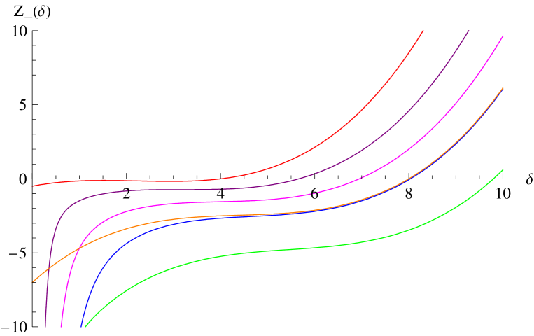
Figure 4: Level crossing of the modes $Z_{-}(\delta)$ from negative to positive values

In anticipation of the general results for the $\eta$–invariant of the Lifshitz operator on Berger spheres, we examine the spectral asymmetry between positive and negative eigen–values in the special cases $\delta=1$ and $\delta=0$. This computation can be done by elementary means and can be used for comparison with the more general formulae that will be derived next. Since there is no spectral asymmetry for $\delta=1$, $\eta_{\mathbb{D}}$ vanishes in this case, as $\eta_{\rm D}$ also does. For $\delta=0$ the finite eigen–values (4.30) are equally distributed to positive and negative values and the same thing applies to all other eigen–values $Z_{\pm}$ that tend to $\pm\infty$. In this case, however, there is an excess of positive modes provided by $Z_{0}$. They have multiplicity $2p$ and depend upon $p$ as $p^{3}$ up to an overall constant $1/(8\delta^{3})$. Although this normalization constant is infinite at $\delta=0$, the $\eta$–invariant does not depend upon it, since $\eta_{\mathbb{D}}$ is inert to uniform rescaling of the spectrum. We immediately find $\eta_{\mathbb{D}}(s)=2\zeta(3s-1)$, and, therefore, $\eta_{\mathbb{D}}=\eta_{\mathbb{D}}(s=0)=2\zeta(-1)=-1/6$. The final result is identical to the $\eta$–invariant of the Dirac operator for $\delta=0$ although in that case the spectrum depends linearly upon $p$ and, thus, $\eta_{{\rm D}}(s)=2\zeta(s-1)$ (see the relevant footnote in Appendix D.3); setting $s=0$ yields the same answer $2\zeta(-1)$ for both operators.

These preliminary results make us suspect that $\eta_{\mathbb{D}}=\eta_{{\rm D}}$ holds for all values of $\delta$ and not only for $0$ and $1$. We will confirm this relation by direct calculation and also explain its occurrence in the context of Atiyah–Patodi–Singer theory that was outlined before.

4.3 Computation of the $\eta$–invariant

In analogy with the Dirac operator discussed in Appendix D.3, we employ the spectral Riemann zeta–function and define the regularized difference between positive and negative eigen–values of the Lifshitz operator by the general formula

$$\eta_{\mathbb{D}}(s)=\sum_{{\rm eigenvalues}}({\rm sign}~{}Z)~{}|Z|^{-s}$$ (4.33)

excluding zero modes. Then, the $\eta$–invariant of the three–dimensional Lifshitz operator is naturally defined by appropriated analytic continuation at $s=0$, as $\eta_{\mathbb{D}}=\eta_{\mathbb{D}}(s=0)$, accounting for its spectral asymmetry.

First, we consider Berger spheres with $\delta<4$ so that $Z_{0}$ and $Z_{+}$ are all positive definite and $Z_{-}$ are all negative. Then, up to uniform rescaling of the spectrum that does not affect the final result for $\eta_{\mathbb{D}}$ (recall that when the spectrum scales uniformly the $\eta$–invariant remains the same because it is evaluated at $s=0$), we have

$$\eta_{\mathbb{D}}(s) = \sum_{p,q>0}(p+q)\left(\left({\delta^{2}\over 2}+X\right)\Big{[}\left({\delta^{2}\over 2}+X\right)^{2}+{\delta^{2}\over 2}(\delta^{2}-4)\Big{]}\right)^{-s}-$$ (4.34)

$$\sum_{p,q>0}(p+q)\left(\left(-{\delta^{2}\over 2}+X\right)\Big{[}\left(-{\delta^{2}\over 2}+X\right)^{2}+{\delta^{2}\over 2}(\delta^{2}-4)\Big{]}\right)^{-s}+$$

$$\sum_{p>0}2p\left(\left({\delta^{2}\over 2}+p\right)\Big{[}\left({\delta^{2}\over 2}+p\right)^{2}+{\delta^{2}\over 2}(\delta^{2}-4)\Big{]}\right)^{-s}$$

setting $X=\sqrt{4\delta^{2}pq+(p-q)^{2}}$ for notational convenience. The first line refers to the contribution of $Z_{+}$, the second to $Z_{-}$ and the third to $Z_{0}$. We will compute the individual sums by expanding all fractions in powers of $\delta$ (up to the appropriate order) and then set $s=0$. The steps we follow are analogous to those outlined in Appendix D.3 for $\eta_{\rm D}$, but, of course, the intermediate expressions are much more involved now.

The contribution of the modes $Z_{0}(\delta)$ is the easiest to evaluate. Using the power series expansion

$$\left(\left({\delta^{2}\over 2}+p\right)\Big{[}\left({\delta^{2}\over 2}+p\right)^{2}+{\delta^{2}\over 2}(\delta^{2}-4)\Big{]}\right)^{-s}=$$

$${1\over p^{3s}}\Big{[}1+{s\delta^{2}\over 2}\left({4\over p^{2}}-{3\over p}\right)+{s(9s-1)\delta^{4}\over 8p^{2}}+\cdots\Big{]}$$ (4.35)

we find that the last term in (4.34) assumes the following expansion in terms of Riemann zeta–functions,

$$\tilde{I}_{0}(s)=2\zeta(3s-1)+s\delta^{2}\left(4\zeta(3s+1)-3\zeta(3s)\right)+{s(9s-1)\delta^{4}\over 4}\zeta(3s+1)+\cdots~{}.$$ (4.36)

The terms that are omitted vanish at $s=0$ since they contain the factor $s\zeta(3s+n)$ with integer $n\geq 2$ and $\zeta(s)$ is absolutely convergent for ${\rm Re}s>1$; they include a term of the form $\delta^{4}/p^{3}$ in (4.35) as well as all terms of order $\delta^{6}$ and higher which come multiplied with $1/p^{n+1}$ with $n\geq 2$. Then, taking into account that $\zeta(-1)=-1/12$, $\zeta(0)=-1/2$ and that $\zeta(s)$ has a simple pole at $s=1$ with residue $1$ (and, thus, $3s\zeta(3s+1)$ equals $1$ at $s=0$), we obtain

$$\tilde{I}_{0}(0)=-{1\over 6}+{4\delta^{2}\over 3}-{\delta^{4}\over 12}~{}.$$ (4.37)

The contribution of the modes $Z_{\pm}(\delta)$ to the $\eta$–invariant is more difficult to extract because of the double sums that are involved. Again, we expand the fractions in power series of $\delta$

$$\left(\left(\pm{\delta^{2}\over 2}+X\right)\Big{[}\left(\pm{\delta^{2}\over 2}+X\right)^{2}+{\delta^{2}\over 2}(\delta^{2}-4)\Big{]}\right)^{-s}={1\over X^{3s}}\Big{[}1+{s\delta^{2}\over 2}\left(\pm{3\over X}+{4\over X^{2}}\right)+$$

$$~{}~{}~{}~{}~{}~{}~{}~{}~{}~{}~{}~{}~{}~{}~{}{s\delta^{4}\over 8}\left({9s-1\over X^{2}}\mp{8(3s+2)\over X^{3}}\right)\mp{3s(s-1)(3s+2)\delta^{6}\over 16X^{3}}+\cdots\Big{]}$$ (4.38)

omitting all terms of the form $1/X^{n+2}$ with $n\geq 2$ that do not contribute to the final result when $s=0$, as will be seen shortly. Then, the first two sums in the general expression (4.34) for $\eta_{\mathbb{D}}(s)$, which we denote respectively by $\tilde{I}_{\pm}(s)$, are expanded as follows,

$$\tilde{I}_{+}(s)-\tilde{I}_{-}(s)=-3s\delta^{2}f\left({3s+1\over 2}\right)-{s(3s+2)\delta^{4}\over 8}\left(16+3(s-1)\delta^{2}\right)f\left({3s+3\over 2}\right)+\cdots~{},$$ (4.39)

when they are combined together, setting for convenience

$$f(s)=\sum_{p,q>0}{p+q\over[4\delta^{2}pq+(p-q)^{2}]^{s}}~{}.$$ (4.40)

The function $f(s)$ also arises in the computation of the $\eta$–invariant of the Dirac operator. It is absolutely convergent on the complex $s$–plane for ${\rm Re}s>3/2$, which justifies the suppression of the higher order terms in the power series expansion (all such terms are multiplied with $s$ and vanish at $s=0$). We also recall from Appendix D.3 that $f(s)$ has simple poles at $s=1/2$ and $s=3/2$ with residues given by equation (D.38). These are the values of $(3s/2)f((3s+1)/2)$ and $(3s/2)f((3s+3)/2)$ at $s=0$ and they are equal to $(\delta^{2}-1)/6$ and $1/(2\delta^{2})$ respectively. Taking these into account, we obtain

$$\tilde{I}_{+}(0)-\tilde{I}_{-}(0)=-\delta^{2}-{\delta^{4}\over 12}~{}.$$ (4.41)

The final result for the $\eta$–invariant of the Lifshitz operator on Berger spheres with $\delta<4$ is identical to the result for the Dirac operator, i.e.,

$$\eta_{\mathbb{D}}=-{1\over 6}(\delta^{2}-1)^{2}~{}.$$ (4.42)

This is not surprising in retrospect because the axial anomaly is identical in both cases including the overall normalization constant. Then, by the Atiyah–Patodi–Singer index theorem, the gravitational Chern–Simons action should be related to the $\eta$–invariant of the Lifshitz operator exactly as the Chern–Simons action is related to $\eta$–invariant of the Dirac operator by equation (D.45). From this point of view, the computation of $\eta_{\mathbb{D}}$ provides an alternative derivation/verification of the axial anomaly for Lifshitz fermions without path integral methods. Hence our interest in pursuing this calculation to the end. It can also be seen here that there are more terms contributing to $\eta_{\mathbb{D}}(s)$, compared to $\eta_{\rm D}(s)$, but they are weighted with different factors. The two expressions are clearly different when $s\neq 0$ (for comparison see the corresponding steps taken in Appendix D.3 for the Dirac operator). Nevertheless, the individual terms add up to produce the same final result at $s=0$, as in the path integral computation of the local form of the axial anomaly.

Next, we consider Berger spheres with $\delta\geq 4$. In analogy with the Dirac operator discussed in Appendix D, let us denote by

$${\cal C}(\delta_{\rm c})=\{(p,q)\in\mathbb{N}^{2};~{}~{}\delta_{\rm c}^{2}=2\sqrt{4pq\delta_{\rm c}^{2}+(p-q)^{2}}\}$$ (4.43)

the set of all positive integers $(p,q)$ associated to zero modes of the Lifshitz operator at each one of the special values $\delta_{\rm c}<\delta$. Since the multiplicity of the zero modes at $\delta_{\rm c}$ is $p+q$ for each $(p,q)$, the quantity

$$S(\delta)=\sum_{\delta_{\rm c}<\delta}\Big{[}\sum_{(p,q)\in{\cal C}(\delta_{\rm c})}(p+q)\Big{]}$$ (4.44)

provides the total number of modes that cross from negative to positive values as $\delta$ varies from $\delta<4$ to any given value $\delta\geq 4$. Taking into account the multiplicity of eigen–values, it follows that $S(\delta)$ is an even integer number. Thus, for $\delta\geq 4$, the $\eta$–invariant of the Dirac operator for Berger spheres is shifted by twice the number of these modes and equals

$$\eta_{\mathbb{D}}=-{1\over 6}(\delta^{2}-1)^{2}+2S(\delta)~{}.$$ (4.45)

$S(\delta)$ is the same number for the Dirac and Lifshitz operators, since level crossing occurs at the same values of $\delta$ and the mode multiplicities are also the same. $S(\delta)$ simply vanishes when $\delta<4$. Thus, we have

$$\eta_{\mathbb{D}}=\eta_{{\rm D}}$$ (4.46)

as advertised above. This formula is actually valid for all $0\leq\delta<\infty$, including the special values $\delta_{\rm c}$, where zero modes appear, and it will be used in the following.

4.4 Chiral symmetry breaking by instantons

We apply the index theorem to the Dirac–Lifshitz operator defined on Hořava–Lifshitz instanton backgrounds with $SU(2)\times U(1)$ isometry. Our treatment is quite general, with no reference to the details of the particular gravitational solutions, in order to identify the sector of the theory that leads to chiral symmetry breaking. As will be seen in the following only the gross qualitative features of the geometry matter for the analytic derivation of the index formula.

Using the Euclidean four–dimensional metric on $M_{4}\simeq\mathbb{R}\times S^{3}$ written in terms of the left–invariant one–forms $\sigma^{I}$ of $SU(2)$ with coefficients $\gamma_{1}=\gamma_{2}\equiv\gamma$,

$$ds^{2}=dt^{2}+\gamma(t)(\sigma^{1})^{2}+\gamma(t)(\sigma^{2})^{2}+\gamma_{3}(t)(\sigma^{3})^{2}~{},$$ (4.47)

we introduce the orthonormal coframe $e^{a}$ of vierbeins given by the one–forms

$$e^{0}=dt~{},~{}~{}~{}~{}~{}e^{1}=\sqrt{\gamma}~{}\sigma^{1}~{},~{}~{}~{}~{}~{}e^{2}=\sqrt{\gamma}~{}\sigma^{2}~{},~{}~{}~{}~{}~{}e^{3}=\sqrt{\gamma_{3}}~{}\sigma^{3}$$ (4.48)

and obtain the corresponding connection one–forms computed by $de^{a}+{\omega^{a}}_{b}\wedge e^{b}=0$,

$${\omega^{0}}_{1}=-{1\over 2\gamma}{d\gamma\over dt}~{}e^{1}~{},~{}~{}~{}~{}~{}{\omega^{0}}_{2}=-{1\over 2\gamma}{d\gamma\over dt}~{}e^{2}~{},~{}~{}~{}~{}~{}{\omega^{0}}_{3}=-{1\over 2\gamma_{3}}{d\gamma_{3}\over dt}~{}e^{3}~{},$$

$${\omega^{2}}_{3}=-{\sqrt{\gamma_{3}}\over 2\gamma}~{}e^{1}~{},~{}~{}~{}~{}~{}~{}{\omega^{3}}_{1}=-{\sqrt{\gamma_{3}}\over 2\gamma}~{}e^{2}~{},~{}~{}~{}~{}~{}~{}{\omega^{1}}_{2}=-{2\gamma-\gamma_{3}\over 2\gamma\sqrt{\gamma_{3}}}~{}e^{3}~{}.$$ (4.49)

Then, the curvature two–forms computed by ${R^{a}}_{b}=d{\omega^{a}}_{b}+{\omega^{a}}_{c}\wedge{\omega^{c}}_{b}$ turn out to be

$${R^{0}}_{1}=-{1\over\sqrt{\gamma}}\left({d^{2}\sqrt{\gamma}\over dt^{2}}\right)e^{0}\wedge e^{1}-{1\over 4\sqrt{\gamma_{3}}}{d\over dt}\left({\gamma_{3}\over\gamma}\right)e^{2}\wedge e^{3}~{},$$ (4.50)

$${R^{0}}_{2}=-{1\over\sqrt{\gamma}}\left({d^{2}\sqrt{\gamma}\over dt^{2}}\right)e^{0}\wedge e^{2}-{1\over 4\sqrt{\gamma_{3}}}{d\over dt}\left({\gamma_{3}\over\gamma}\right)e^{3}\wedge e^{1}~{},$$ (4.51)

$${R^{0}}_{3}=-{1\over\sqrt{\gamma_{3}}}\left({d^{2}\sqrt{\gamma_{3}}\over dt^{2}}\right)e^{0}\wedge e^{3}+{1\over 2\sqrt{\gamma_{3}}}{d\over dt}\left({\gamma_{3}\over\gamma}\right)e^{1}\wedge e^{2}~{},$$ (4.52)

$${R^{2}}_{3}=-{1\over 2\sqrt{\gamma}}\left({d\over dt}\sqrt{{\gamma_{3}\over\gamma}}\right)e^{0}\wedge e^{1}+{1\over 4\gamma\gamma_{3}}\left({\gamma_{3}^{2}\over\gamma}-{d\gamma\over dt}{d\gamma_{3}\over dt}\right)e^{2}\wedge e^{3}~{},$$ (4.53)

$${R^{3}}_{1}=-{1\over 2\sqrt{\gamma}}\left({d\over dt}\sqrt{{\gamma_{3}\over\gamma}}\right)e^{0}\wedge e^{2}+{1\over 4\gamma\gamma_{3}}\left({\gamma_{3}^{2}\over\gamma}-{d\gamma\over dt}{d\gamma_{3}\over dt}\right)e^{3}\wedge e^{1}~{},$$ (4.54)

$${R^{1}}_{2}={1\over 2\sqrt{\gamma_{3}}}{d\over dt}\left({\gamma_{3}\over\gamma}\right)e^{0}\wedge e^{3}-{1\over 4\gamma^{2}}\left(3\gamma_{3}-4\gamma+\left({d\gamma\over dt}\right)^{2}\right)e^{1}\wedge e^{2}$$ (4.55)

and after some calculation the topological density takes the form of a total derivative term, without using any equations of motion,

$${\rm Tr}(R\wedge R)={d\over dt}~{}\Big{[}~{}{1\over 2}\gamma_{3}\left({d\over dt}{\rm log}{\gamma_{3}\over\gamma}\right)^{2}+\left({\gamma_{3}\over\gamma}-1\right)^{2}\Big{]}~{}dt\wedge\sigma^{1}\wedge\sigma^{2}\wedge\sigma^{3}.$$ (4.56)

We also introduce a variant of the four–dimensional metric that has the cross–product form

$$ds_{(0)}^{2}=dt^{2}+\gamma(t_{0})(\sigma^{1})^{2}+\gamma(t_{0})(\sigma^{2})^{2}+\gamma_{3}(t_{0})(\sigma^{3})^{2}~{},$$ (4.57)

using a fixed parameter $t_{0}$ instead of $t$ in the metric components. It serves as reference frame for the computations in the vicinity of $t=t_{0}$. Since the connection one–forms of the cross–product metric have components ${\omega^{0}}_{i}=0$ and ${\omega^{i}}_{j}$ are the same as above with $t$ simply replaced by $t_{0}$, we infer that the second fundamental form $\theta=\omega-\omega_{0}$ has the following non–vanishing components at $t=t_{0}$,

$${\theta^{0}}_{1}=-{d\sqrt{\gamma}\over dt}|_{t=t_{0}}~{}\sigma^{1}~{},~{}~{}~{}~{}~{}~{}{\theta^{0}}_{2}=-{d\sqrt{\gamma}\over dt}|_{t=t_{0}}~{}\sigma^{2}~{},~{}~{}~{}~{}~{}~{}{\theta^{0}}_{3}=-{d\sqrt{\gamma_{3}}\over dt}|_{t=t_{0}}~{}\sigma^{3}~{}.$$ (4.58)

Then, ${\rm Tr}(\theta\wedge R)$ at any given slice $t=t_{0}$ is given by

$${\rm Tr}(\theta\wedge R)|_{t=t_{0}}={1\over 2}\gamma\left({d\over dt}{\rm log}{\gamma_{3}\over\gamma}\right){d\over dt}\left({\gamma_{3}\over\gamma}\right)|_{t=t_{0}}~{}\sigma^{1}\wedge\sigma^{2}\wedge\sigma^{3}~{}.$$ (4.59)

Applying the Atiyah–Patodi–Singer index theorem (4.5) to the fermion operator ${\cal D}$ (it can be either $D$ or $\mathbb{D}$) we obtain

$${\rm Ind}({\cal D}) = -{1\over 12}~{}\Big{[}~{}{1\over 2}\gamma_{3}\left({d\over dt}{\rm log}{\gamma_{3}\over\gamma}\right)^{2}+\left({\gamma_{3}\over\gamma}-1\right)^{2}\Big{]}_{t=-\infty}^{t=+\infty}+$$ (4.60)

$${1\over 24}\Big{[}~{}\gamma\left({d\over dt}{\rm log}{\gamma_{3}\over\gamma}\right){d\over dt}\left({\gamma_{3}\over\gamma}\right)\Big{]}_{t=-\infty}^{t=+\infty}-{1\over 2}\Big{[}\eta_{\cal D}\Big{]}_{t=-\infty}^{t=+\infty}$$

after performing the integral in the time variable $t$ and the angular coordinates of $S^{3}$, using the volume element $\sigma^{1}\wedge\sigma^{2}\wedge\sigma^{2}={\rm sin}\theta~{}d\theta\wedge d\varphi\wedge d\psi$, which yields a factor of $16\pi^{2}$. This result is quite general, as it stands, because it does not depend on the specific form of the metric coefficients $\gamma(t)$ and $\gamma_{3}(t)$ for intermediate times, but it relies on their existence as $t$ varies from $-\infty$ to $+\infty$.

Furthermore, we observe that the time derivative terms cancel against each other without reference to any field equations, and, thus, equation (4.60) simplifies to

$${\rm Ind}({\cal D})=-{1\over 12}~{}\Big{[}\left({\gamma_{3}\over\gamma}-1\right)^{2}\Big{]}_{t=-\infty}^{t=+\infty}-{1\over 2}\Big{[}\eta_{\cal D}\Big{]}_{t=-\infty}^{t=+\infty}~{}.$$ (4.61)

The only information needed for computing the index are the boundary values of the metric coefficients, whereas the boundary values of their time derivatives are irrelevant. Thus, this formula is equally valid for the instantons of Hořava–Lifshitz gravity that interpolate between any two fixed points of the Ricci–Cotton flow with $\delta=1$ and $0<\delta\neq 1$ as well as for the instantons that extend all the way to the fully squashed sphere with $\delta=0$. Setting $\gamma_{3}/\gamma=\delta^{2}$, as we did before, and using the general expression for the $\eta$–invariant on Berger spheres, $\eta_{\cal D}=-(\delta^{2}-1)^{2}/6+2S(\delta)$, we arrive at the final expression

$${\rm Ind}({\cal D})=-\Delta S$$ (4.62)

given by the number of level crossings (including their multiplicities) that have occurred on the spatial slices, via deformation of $\delta$, in the entire history of time (for the definition of $S(\delta)$ see equation (4.44) or (D.47)). This is precisely what was expected by the spectral flow argument. Instantons and anti–instantons will have opposite signs of $\Delta S$, if it is not zero, since they are mutually related by $t\rightarrow-t$. It is also obvious now that the index vanishes on all instanton backgrounds whose end–points have non–negative sectional Ricci scalar curvature.

The only instantons that can give rise to level crossing, and, thus, to non–vanishing index occur in the unimodular version of Hořava–Lifshitz gravity with superspace parameter $\lambda=1/3$. They are eternal solutions of the normalized Ricci–Cotton flow whose end–points are not constrained to have the same Ricci scalar curvature. When, in particular, the Chern–Simons parameter $\omega$ is negative (for a given choice of orientation on $S^{3}$), there are flow lines that interpolate between the totally isotropic configuration and a Berger metric with anisotropy parameter

$$\delta^{2}\equiv a^{3}=\left(-{\omega L\over 3\kappa_{\rm w}^{2}}\right)^{3/2}~{}.$$ (4.63)

Recall from section 3.3 (to which we refer for the notation) that such chiral instantons are associated to the tunneling of an effective point–particle between the red bullet vacua of the potential well shown in Fig.2c and Fig.2d; as such, they correspond to continuous deformations of the round sphere to configurations with $\delta<1$ and $\delta>1$, respectively.

The necessary and sufficient condition to have non–vanishing index is provided by $\delta>4$, which singles out Fig.2d with the left red bullet pushed sufficiently far away from the origin. This, in turn, amounts to the following inequality among the various parameters of the theory,

$$-{\omega\over\kappa_{\rm w}^{2}}>24\left({\pi^{2}\over{\rm Vol}(S^{3})}\right)^{1/3}.$$ (4.64)

Here, we have expressed the characteristic length scale (size) $L$ of space in terms of the volume of $S^{3}$ which equals to $2\pi^{2}L^{3}$ and it remains constant in time. Then, the index is given by the total number of modes that changed sign as $\delta$ was varying from $1$ to $a^{3/2}$ and equals

$${\rm Ind}({\cal D})=\pm S(a^{3/2})$$ (4.65)

with plus or minus signs referring to the way that the cylinder $\mathbb{R}\times S^{3}$ is transversed (backward or forward in Euclidean time). This is in agreement with the spectral flow interpretation of the index of the spin complex.

In more physical terms, a non–vanishing index implies that the axial charge associated to the (anomalous) conservation law of the axial current $J_{5}^{\mu}$,

$$Q_{5}=\int_{\Sigma_{3}}d^{3}x\sqrt{{\rm det}g}~{}J_{5}^{0}(t,x)~{},$$ (4.66)

is not necessarily conserved but it rather changes as

$$\Delta Q_{5}={\rm Ind}({\cal D})$$ (4.67)

in all processes mediated by the corresponding gravitational instanton backgrounds and it leads to lepton and baryon number non–conservation. The index is an integer number (this is consistent with the fact that $M_{4}$ admits spin structure), which can become arbitrarily large when the parameter $a$ is sufficiently large. In terms of the inequality (4.64), it implies that Hořava–Lifshitz gravity can exhibit chiral symmetry breaking when the relative coupling of the Cotton term ($\sim\kappa_{\rm w}/\omega$) is sufficiently small. Said differently, chiral symmetry breaking becomes possible when there is a lower bound on the volume of space for fixed couplings $\kappa_{\rm w}$ and $\omega$,

$${\rm Vol}(S^{3})>13824\pi^{2}\left(-{\kappa_{\rm w}^{2}\over\omega}\right)^{3}.$$ (4.68)

A Lifshitz universe that exhibits a bounce [67, 68, 69] may help to realize this novel possibility in practice. We intend to study the implications of this scenario elsewhere in more detail.

Another interesting question is the behavior of inequality (4.68) for chiral symmetry breaking under the renormalization group equations of topologically massive gravity. The one–loop beta functions for the three dimensional Newton coupling $\kappa_{\rm w}^{2}$ and the cosmological constant $\Lambda$ have been computed explicitly in the recent paper [70], where it was also found that the Chern–Simons coupling $\omega$ does not change with the energy scale. One may try to recast these results into a form that is directly applicable to the unimodular variant of topologically massive gravity, in which $\Lambda$ assumes the role of an integration constant and the volume of three–space appears as a running coupling, and inquire whether both sides of the inequality (4.68) are renormalization group invariant (at least to one–loop level). It seems that the answer is negative. A weaker (and perhaps more appropriate) question that can be posed in this context is whether the inequality (4.68) is not overturned by the renormalization group flow once it is satisfied at a given energy scale; and if so, what will be the deeper meaning of this? We are primarily interested in studying this question in the vicinity of a non–trivial fixed point, which is UV attractive in all directions and has negative $\Lambda$, but there are still some issues left open in the analysis given in [70] that prevent us from drawing definite conclusions at this moment. Intertwining our results with renormalization group ideas and exploring their meaning in the four–dimensional theory of Hořava–Lifshitz gravity are some important problems to which we also hope to return elsewhere.

4.5 Topological invariants of the instantons

The index of the Dirac–Lifshitz operator on our gravitational instanton backgrounds is not a topological invariant of space–time. This is mere reflection of the fact that the dimension of the space of harmonic spinors on $S^{3}$ is not bounded by the topology. It only depends on the geometry and it can grow without bound for metrics with very negative Ricci scalar curvature. Thus, to complete our discussion, we will compute explicitly the topological numbers of the instanton spaces, namely their signature and Euler numbers, using the Atiyah–Patodi–Singer theorem for the Hirzebruch and de Rham complexes, respectively. They both turn out to be zero, as expected by the cylindrical form of $M_{4}$ (but see also the exact arguments below).

Hirzebruch signature complex: The signature of a Riemannian four–manifold with boundaries is closely related to the formula for the index of the fermion operator. It reads [19]

$$\tau(M_{4})=-{1\over 24\pi^{2}}\int_{M_{4}}{\rm Tr}(R\wedge R)+{1\over 24\pi^{2}}\int_{\partial M_{4}}{\rm Tr}(\theta\wedge R)-\eta_{\rm S}(\partial M_{4})~{}.$$ (4.69)

The first two terms are identical to those appearing in (4.5) for ${\rm Ind}({\cal D})$, but they are now multiplied with $1/24\pi^{2}$ that differs from $1/192\pi^{2}$ by a factor of $8$ (this is also consistent with the fact that a compact four–dimensional spin manifold without boundaries has signature that is an integer multiple of $8$). Thus, their particular form is known from before (see equations (4.56) and (4.59)). The last term is the associated $\eta$–invariant for the signature complex, which has been computed by Hitchin on Berger spheres [71] and takes the following form,

$$\eta_{\rm S}(\delta)=-{2\over 3}(\delta^{2}-1)^{2}$$ (4.70)

for all values of the anisotropy parameter $\delta$. Since it is also $8$ times larger than $\eta_{\cal D}/2=-(\delta^{2}-1)^{2}/12$, without counting the effect of level crossing, as it does not occur here, we find immediately that $\tau(M_{4})=0$.

Euler–de Rham complex: The Euler number of a Riemannian four–manifold with boundaries is given by

$$\chi(M_{4})={1\over 32\pi^{2}}\int_{M_{4}}\epsilon_{abcd}~{}{R^{a}}_{b}\wedge{R^{c}}_{d}-{1\over 16\pi^{2}}\int_{\partial M_{4}}\epsilon_{abcd}\left({\theta^{a}}_{b}\wedge{R^{c}}_{d}-{2\over 3}{\theta^{a}}_{b}\wedge{\theta^{c}}_{e}\wedge{\theta^{e}}_{d}\right).$$ (4.71)

The bulk term is the integral of the Gauss–Bonnet topological density and the boundary term is the integral of the corresponding Chern–Simons secondary class which is required for well definiteness. In this case there is no analogue of the $\eta$–invariant boundary term. Explicit computation shows that all our gravitational instanton backgrounds obey the following relation,

$${1\over 2}\epsilon_{abcd}~{}{R^{a}}_{b}\wedge{R^{c}}_{d}=\epsilon_{abcd}~{}dt\wedge{d\over dt}\left({\theta^{a}}_{b}\wedge{R^{c}}_{d}-{2\over 3}{\theta^{a}}_{b}\wedge{\theta^{c}}_{e}\wedge{\theta^{e}}_{d}\right)=$$ (4.72)

$${d\over dt}~{}\Big{[}~{}{1\over 2\gamma\sqrt{\gamma_{3}}}\left(\left({d\gamma\over dt}\right)^{2}-4\gamma+3\gamma_{3}\right)\left({d\gamma_{3}\over dt}\right)-{(\sqrt{\gamma_{3}})^{3}\over\gamma^{2}}\left({d\gamma\over dt}\right)\Big{]}~{}dt\wedge\sigma^{1}\wedge\sigma^{2}\wedge\sigma^{3},$$

and, therefore, we easily obtain that $\chi(M_{4})=0$. This relation follows from the particular form of the four–dimensional metric $ds^{2}=dt^{2}+\gamma(t)(\sigma^{1})^{2}+\gamma(t)(\sigma^{2})^{2}+\gamma_{3}(t)(\sigma^{3})^{2}$ without using any equations of motion.

Another way to view these results is to think of $M_{4}\simeq\mathbb{R}\times S^{3}$ as being topologically equivalent to a compact manifold $M_{\rm c}\simeq S^{4}$ with two points removed, say the "north" and the "south" poles. This is best seen by considering the canonical de Sitter metric on $S^{4}$ with radius $L$ and $r$ running from $0$ to $\infty$,

$$ds^{2}={1\over(1+(r/2L)^{2})^{2}}\Big{[}~{}dr^{2}+4r^{2}\left((\sigma^{1})^{2}+(\sigma^{1})^{2}+(\sigma^{1})^{2}\right)\Big{]}~{}.$$ (4.73)

Passing to the proper coordinate $t$ given by the change of variables ${\rm tan}(t/2L)=r/2L$, the metric takes the form

$$ds^{2}=dt^{2}+{\rm sin}^{2}\left({t\over L}\right)\left((\sigma^{1})^{2}+(\sigma^{1})^{2}+(\sigma^{1})^{2}\right)$$ (4.74)

with $t$ running from $0$ to $\pi L$. It resembles the form of the four–dimensional metrics that we have been considering all along having homogeneous and isotropic slices with $\gamma_{1}=\gamma_{2}=\gamma_{3}={\rm sin}^{2}(t/L)$. In this frame, $S^{4}$ is described as $S^{1}$ fibration over $S^{3}$. At the two poles which are located at $t=0$ and $\pi L$, respectively, the three–dimensional slices shrink to a point. Then, removing the two poles yields a compact space with boundaries that has the topology of $\mathbb{R}\times S^{3}$. Next, using the following general relations $\tau(M_{4})=\tau(M_{\rm c})$ and $\chi(M_{4})=\chi(M_{\rm c})-2$, and knowing, in particular, that $\tau(S^{4})=0$ and $\chi(S^{4})=2$, we obtain immediately that $\tau(M_{4})=0=\chi(M_{4})$.

It is now appropriate to compare these results to the topological invariants of instanton solutions of Einstein gravity, focusing, in particular, to the Taub–NUT and Eguchi–Hanson spaces. These metrics take exactly the same form in proper time as the instantons of Hořava–Lifshitz gravity, and, therefore, one may (erroneously) think that their signature and Euler numbers also vanish. Here, we focus to the topological aspects of these spaces (their analytic properties are discussed in the next section to which we refer for details) and explain in brief how the presence of removable singularities affects the computation of $\chi$ and $\tau$. Such singularities are not present in the instanton metrics of Hořava–Lifshitz gravity, by construction, and, naturally both $\chi$ and $\tau$ vanish there.

The removable singularities that arise at one end of the instanton solutions of Einstein gravity form the fixed point set of a Killing vector field. Then, one has to employ the Lefschetz fixed–point theorem, which is a special case of the more general $G$–index theorem, to account for the presence of the fixed points in the computation of the Euler number (see, for instance, [29] for a rather elementary account). According to this theorem, an isolated fixed point (nut) adds one unit to the Euler number of the manifold and a surface of fixed points that form an invariant $S^{2}$ submanifold (bolt) adds to it two units. As a result, the Euler number of Taub–NUT space is $1$ and that of Eguchi–Hanson space is $2$. The computation of the signature requires some additional ingredients in the case of Eguchi–Hanson space: the $\eta$-invariant of the signature complex (4.70) should be made equivariant with respect to a discrete $\mathbb{Z}_{2}$ symmetry that identifies antipodal points on $S^{3}$ (see, for instance, [71]) and integration over $S^{3}$ yields a factor of $8\pi^{2}$ instead of $16\pi^{2}$. Taking these into account one finds that the signature of Eguchi–Hanson space is $\pm 1$ (the sign refers to the choice of instanton or anti–instanton metric), whereas the signature of Taub–NUT space vanishes. In either case we have $\chi(M_{4})=|\tau(M_{4})|+1$, as required on general grounds for this class of Einstein spaces.

5 Comparison to relativistic theories

This section is devoted to instanton solutions of Einstein gravity and the associated index formulae for the Dirac operator. It will make more transparent the issues we addressed earlier but in a more familiar context.

The index of the Dirac operator $D$ in the background of a four–dimensional metric on a manifold $M_{4}$ with boundary $\partial M_{4}$ takes the same form (4.5) as for the Lifshitz operator, according to Atiyah–Patodi–Singer index theorem [19], where $\eta_{\rm D}$ is the $\eta$–invariant of the three–dimensional Dirac operator at the boundary, which is discussed extensively in Appendix D. ${\rm Ind}(D)$ counts the difference in the number of normalizable positive and negative chirality spinors obeying the appropriate boundary conditions, as usual. Our main objective is to compute the index of the Dirac operator in the background of Taub–NUT [21] and Eguchi–Hanson [22] gravitational instanton metrics so that direct comparison can be made to the results derived in the non–relativistic case. Our exposition is somewhat extensive containing all relevant details and it includes a relatively new (alternative) derivation of the index in the case of Eguchi–Hanson space.

5.1 Gravitational instantons with $SU(2)\times U(1)$ isometry

The Taub–NUT and Eguchi–Hanson metrics provide the only complete and regular gravitational instanton solutions of Einstein gravity with $SU(2)\times U(1)$ group of isometries. They also admit an effective point particle description in the context of mixmaster dynamics [60] that parallels the description of $SU(2)\times U(1)$ instantons of Hořava–Lifshitz gravity.

Recall that the potential of general relativity is minus the Ricci scalar curvature of the spatial slices $\Sigma_{3}$ in the ADM formulation of the theory on $\mathbb{R}\times\Sigma_{3}$ [44]. Using the Bianchi IX ansatz, we find that the gravitational action with metric coefficients (3.30) takes the following form in proper time (with $N(t)=1$),

$$S_{\rm eff.}={6\pi^{2}\over\kappa^{2}}\int dt~{}e^{3\Omega}~{}\Big{[}\left({d\beta\over dt}\right)^{2}-4\left({d\Omega\over dt}\right)^{2}-{16\over 3}e^{-2\Omega}\left(e^{-4\beta}-4e^{-\beta}\right)\Big{]}~{},$$ (5.1)

setting for convenience $\kappa^{2}=32\pi G$ and

$$\beta={\rm log}x~{},~{}~{}~{}~{}~{}~{}\Omega={\rm log}L~{}.$$ (5.2)

Note that the superspace metric is not positive definite for Einstein gravity, since one has to take $\lambda=1$, [49], and this is reflected in the negative kinetic energy of the volume modulus found in the effective action. Because of this difference, the instantons of Einstein gravity admit a slightly different description (compared to the instantons of Hořava–Lifshitz theory), which is not directly based on Euclidean action bounds. Now the action can in principle be made arbitrarily negative because of the indefiniteness of the DeWitt metric associated to the conformal factor. Yet, the Euclidean action of Einstein instantons is finite and it is given by a boundary term, since the bulk term vanishes. Also, the instantons of Einstein gravity have self–dual Riemann curvature tensor, whereas in Hořava–Lifshitz theory self–duality is not present.

Fig.5 is a plot of the effective potential $V(\beta)$ appearing in the action (5.1) as function of the anisotropy parameter $\beta$ with fixed $\Omega$.

Figure 5: Effective potential for $SU(2)\times U(1)$ mixmaster dynamics in Einstein gravity

In this case, however, the volume of space changes with time and $V(\beta)$ scales appropriately. The plot is closely related to the one shown in Fig.3 for $R(x)$, since $V=-R$, but the potential is now expressed as function of $\beta$ rather than $x$. It should also be compared to the form of the potential in Hořava–Lifshitz gravity. All these differences will be explained next from a particular point of view.

Following [18], we invert the potential $V(\beta)$ and represent an $SU(2)\times U(1)$ instanton by a point particle which rolls from the top of the hill located at $\beta=0$ towards the plateau that is reached asymptotically as $\beta\rightarrow+\infty$. But the potential also varies with time through its scaling factor, thus adjusting continuously the height difference in the course of the motion. More importantly, the two end–points of the particle trajectory have $\Omega=\pm\infty$. The top of the hill will correspond to a removable nut singularity in space–time if $\Omega=-\infty$ and to a Euclidean (or conical infinity) if $\Omega=+\infty$. Likewise, the plateau reached at the other end of the motion will correspond to a removable bolt singularity in space–time if $\Omega=-\infty$ and to a Taubian infinity if $\Omega=+\infty$. As a matter of fact, the self–dual Taub–NUT metric corresponds to a trajectory which starts with zero velocity at the top of the hill as $\Omega=-\infty$ and reaches the plateau at infinity as $\Omega=+\infty$. On the other hand, the Eguchi–Hanson instanton corresponds to a trajectory that starts from the plateau at infinity as $\Omega=-\infty$ and reaches the top of the hill as $\Omega=+\infty$. These are the only two possible instanton solutions of Einstein gravity with $SU(2)\times U(1)$ isometry that yield complete non–singular manifolds. In both these cases, the proper time variable $t$ extends from a finite value (say $0$) to $+\infty$ since there is a nut or a bolt forming at $t=0$ and space–time ends there. The anti–instantons follow by letting $t\rightarrow-t$.

This qualitative picture can be made precise by writing down the first order equations that $\beta$ and $\Omega$ satisfy in time. They are gradient flow equations derived from a superpotential which is the Hamilton–Jacobi functional of general relativity computed for Bianchi IX metrics. In our case, the potential takes the form

$${16\over 3}e^{-2\Omega}\left(e^{-4\beta}-4e^{-\beta}\right)=e^{-6\Omega}\Big{[}\left({\partial{\cal W}\over\partial\beta}\right)^{2}-{1\over 4}\left({\partial{\cal W}\over\partial\Omega}\right)^{2}\Big{]}$$ (5.3)

and the first order equations satisfied by the instantons are

$${d\beta\over dt}=\pm e^{-3\Omega}~{}{\partial{\cal W}\over\partial\beta}~{},~{}~{}~{}~{}~{}4{d\Omega\over dt}=\mp e^{-3\Omega}~{}{\partial{\cal W}\over\partial\Omega}~{}.$$ (5.4)

Note, however, that ${\cal W}$ is not uniquely determined because of the indefiniteness of the DeWitt metric. There are two possible choices of superpotential given by

$${\cal W}_{\rm TN}={4\over 3}~{}e^{2\Omega}\left(e^{-2\beta}-4e^{-\beta/2}\right)~{}~{}~{}~{}~{}~{}~{}{\rm or}~{}~{}~{}~{}{\cal W}_{\rm EH}={4\over 3}~{}e^{2\Omega}\left(e^{-2\beta}+2e^{\beta}\right),$$ (5.5)

which correspond to the celebrated Taub–NUT and Eguchi–Hanson instantons, respectively. In the first case, ${\rm exp}(-2\Omega+2\beta)-{\rm exp}(-2\Omega+\beta/2)=1/(16m^{2})$ is a first integral of the system (5.4) and the integration constant $m$ is called nut parameter. In the second case, the integral is provided by ${\rm exp}(4\Omega+2\beta)-{\rm exp}(4\Omega-\beta)=a^{4}$ with $a$ being the modulus of Eguchi–Hanson metric. These integrals allow to determine the metric of gravitational instantons in closed form.

It can be easily verified that the first order equations (5.4) solve the second order equations of motion following from the action (5.1) upon analytic continuation in time. The relative minus sign between $(\partial{\cal W}/\partial\beta)^{2}$ and $(\partial{\cal W}/\partial\Omega)^{2}$ in the potential is also attributed to the indefiniteness of the DeWitt metric. The plus or minus signs appearing in the defining relations (5.4) refer to the instanton or anti–instanton configurations, which are related to each other by time reversal. These equations also follow from the self–duality relations by integrating once in time and making the appropriate choice of integration constants (we refer the reader to the original work [18] for these technical details). It so happens that the first order equations for the metric coefficients of the self–dual Taub–NUT space are identical to the Ricci flow equations on $S^{3}$ with metric (3.28) provided that $\gamma_{i}$ are traded with $\gamma_{i}^{2}$. There is no analogous interpretation of the equations that determine the Eguchi–Hanson metric.

The Euclidean point particle action for these trajectories is evaluated by completing the squares and using equation (5.4). We obtain

$$S_{\rm instanton}=\pm{12\pi^{2}\over\kappa^{2}}\int dt\left({\partial{\cal W}\over\partial\beta}{d\beta\over dt}+{\partial{\cal W}\over\partial\Omega}{d\Omega\over dt}\right)=\pm{12\pi^{2}\over\kappa^{2}}\int dt~{}{d{\cal W}\over dt}=\pm{12\pi^{2}\over\kappa^{2}}\Delta{\cal W}~{},$$ (5.6)

which is solely determined by the difference of ${\cal W}$ at the end points of proper time, $t=0$ and $\pm\infty$. As such, it resembles the form of the action for Hořava–Lifshitz instantons. However, ${\cal W}$ blows up in the asymptotic region of both instanton solutions (Taubian or conical infinity). This can be easily seen by employing the first integrals and evaluating ${\cal W}$ at $t=\pm\infty$. At the other end of the instanton, which corresponds to a removable singularity (nut or bolt) reached at $t=0$, ${\cal W}$ is finite. Thus, $S_{\rm instanton}$, as evaluated above, turns out to be infinite and looks problematic. To remedy the situation one has to subtract the infinite contribution of the flat space metric which serves as reference frame in the calculations.

Notice in this respect that the integral of the mean curvature of any given slice $\Sigma_{3}$ is the derivative of its volume, which, in turn yields the following relation using the first order equations (5.4),

$$\int_{\Sigma_{3}}d^{3}x\sqrt{{\rm det}g}~{}K={1\over 2}\int_{\Sigma_{3}}d^{3}x\sqrt{{\rm det}g}~{}g^{ij}{d\over dt}g_{ij}={d\over dt}{\rm Vol}(\Sigma_{3})=2\pi^{2}{d\over dt}e^{3\Omega}=\mp 3\pi^{2}{\cal W}~{}.$$ (5.7)

The mean curvature is the trace of the extrinsic curvature, $K=g^{ij}K_{ij}$, with $2K_{ij}=dg_{ij}/dt$ since we have made the choice of lapse and shift functions $N=1$ and $N_{i}=0$. The volume of space is ${\rm Vol}(\Sigma_{3})=2\pi^{2}L^{3}$ with $L={\rm exp}\Omega$, and, finally, we have $\partial{\cal W}/\partial\Omega=2{\cal W}$ due to the particular dependence of ${\cal W}$ upon $\Omega$ for both Taub–NUT and Eguchi–Hanson spaces. Based on this observation, we recast the Euclidean instanton action (5.6) in the form

$$S_{\rm instanton}=-{4\over\kappa^{2}}\int_{\partial M_{4}}d^{3}x\sqrt{{\rm det}g}~{}K~{}.$$ (5.8)

To make the action finite one simply has to subtract the contribution of a reference round sphere with volume $16\pi^{2}t^{3}$ at both ends of space–time which we write as

$$S_{\rm instanton}^{\prime}=-{4\over\kappa^{2}}\int_{\partial M_{4}}d^{3}x\sqrt{{\rm det}g}~{}(K-K_{0})~{}.$$ (5.9)

The integral of $K-K_{0}$ over $\partial M_{4}$ is precisely the so called Gibbons–Hawking boundary term and it is rewarding to derive it here in the canonical ADM formalism by a different line of arguments. Taking this into account, the regulated instanton action of the Eguchi–Hanson metric turns out to be zero and the difference in the normalization of $S_{\rm eff.}$ (being $8\pi^{2}$ instead of $16\pi^{2}$) becomes irrelevant. The regulated action of Taub–NUT instanton is not zero but finite.

Recall for completeness that in the conventional approach to the problem one adds the Gibbons–Hawking boundary term to the bulk Einstein–Hilbert action [72] (but see also [73]). This is provided by the difference between the trace of the second fundamental form of the boundary in a given metric, $K$, and its value in the flat space metric, $K_{0}$. More precisely, we have the Euclidean action (setting $\kappa^{2}=32\pi G$, as before)

$$S_{{\rm gravity}}=-{2\over\kappa^{2}}\int_{M_{4}}d^{4}x\sqrt{{\rm det}G}~{}R[G]-{4\over\kappa^{2}}\int_{\partial M_{4}}d^{3}x\sqrt{{\rm det}g}~{}(K-K_{0})~{}.$$ (5.10)

This does not affect the classical equations of motion but it makes the variational problem well–posed in the presence of boundaries. Then, the Euclidean action of the instanton metrics is provided by the Gibbons–Hawking boundary term alone, since the bulk term vanishes, and it is finite, as required on general grounds.

In summary, the instantons of Einstein gravity with $SU(2)\times U(1)$ isometry resemble the instantons of Hořava–Lifshitz gravity that interpolate between the round and a fully squashed sphere. The volume of their spherical slices is modulated with time. In the non–relativistic case the extrinsic curvature vanishes at the end–points of space–time, since these are the fixed points of the Ricci–Cotton flow, and the Gibbons–Hawking term becomes obsolete. Nevertheless, it will be interesting to investigate the form of the boundary terms in Hořava–Lifshitz gravity in more general situations.

5.2 Index of Dirac operator for Taub–NUT metric

The Taub–NUT metric is conveniently written in terms of a radial coordinate $r\in[m,\infty)$ ($m$ is the nut parameter) as

$$ds_{\rm TN}^{2}={r+m\over r-m}dr^{2}+(r^{2}-m^{2})\Big{[}(\sigma^{1})^{2}+(\sigma^{2})^{2}+{4m^{2}\over(r+m)^{2}}(\sigma^{3})^{2}\Big{]}~{}.$$ (5.11)

The end–points of $r$ determine the two boundaries of Taub–NUT space: the removable nut singularity and the asymptotic infinity. Proper time can be alternatively used, setting

$$\pm t=\int_{m}^{r}dx\sqrt{{x+m\over x-m}}=m~{}{\rm arcosh}~{}{r\over m}+\sqrt{r^{2}-m^{2}}~{},$$ (5.12)

and it runs from $0$ to $\pm\infty$ (the sign depends on whether one imposes self–duality or anti–self–duality condition on the Riemann tensor). As for the three Euler angles that are used to represent $\sigma^{i}$, they range as $0\leq\theta\leq\pi$, $0\leq\varphi\leq 2\pi$, $0\leq\psi\leq 4\pi$, and, therefore, the slices that arise at fixed $r$ have the topology of $S^{3}$ ($\psi$ is extended to the double covering of the rotation group $SO(3)$). Thus, integrating the volume form $\sigma^{1}\wedge\sigma^{2}\wedge\sigma^{3}={\rm sin}\theta~{}d\theta\wedge d\varphi\wedge d\psi$ yields a factor $16\pi^{2}$.

The computation of the index of the Dirac operator $D$ on the Taub–NUT space relies on the general formula that was obtained in section 4 without reference to any equations of motion for the background geometry. Using equations (4.56) and (4.59), we have, in particular,

$${\rm Ind}(D)=-{1\over 12}~{}\Big{[}\left({\gamma_{3}\over\gamma}-1\right)^{2}\Big{]}_{r=m}^{r=+\infty}-{1\over 2}\Big{[}\eta_{\rm D}\Big{]}_{r=m}^{r=+\infty}~{}.$$ (5.13)

The derivation of equations (4.56) and (4.59) was done before using the proper (Euclidean) time $t$, but it can also be done using the radial coordinate $r$. The only difference is that the end–points of the instanton are now located at $r=m$ and $r=\infty$ (equivalently at $t=0$ and $t=\infty$) as shown above.

Here, the slices arising at fixed $r$ are Berger spheres with anisotropy parameter

$${\gamma_{3}\over\gamma}=\delta^{2}={4m^{2}\over(r+m)^{2}}$$ (5.14)

and the $\eta$–invariant takes the following form, according to formula (D.42),

$$\eta_{\rm D}|_{r}=-{(r+3m)^{2}(r-m)^{2}\over 6(r+m)^{4}}~{}.$$ (5.15)

Note that $\eta_{\rm D}|_{r=m}=0$, since the nut is conformally related to an $S^{3}$ endowed with the constant curvature metric (i.e., $\delta=1$). We also note that $\eta_{\rm D}|_{r=\infty}=-1/6$, since the Taubian infinity is conformally related to the fully squashed $S^{3}$ (i.e., $\delta=0$). These special cases are discussed in detail in Appendix D and they provide the two extreme values of $\delta$ in Taub–NUT space.

We have, in particular, $\delta\leq 1$ so that the spherical slices have positive Ricci scalar curvature for all $r\geq m$. Thus, there is no level crossing from negative to positive eigen–values of the three–dimensional Dirac operator as the slices are deforming geometrically by varying $r$ and the index vanishes. This is also apparent from equation (5.13). Thus, there is no chiral symmetry breaking induced by this gravitational instanton background reconfirming the results that were originally obtained in the literature [23, 24] long time ago. The Hirzebruch signature of Taub–NUT space is eight times the index of the Dirac operator – there are no caveats in this case – and it vanishes, as noted before.

5.3 Index of Dirac operator for Eguchi–Hanson metric

Another example is provided by the Eguchi–Hanson metric which is conveniently written using a radial coordinate $r\in[a,\infty)$ as

$$ds_{\rm EH}^{2}={dr^{2}\over 1-a^{4}/r^{4}}+{r^{2}\over 4}~{}\Big{[}(\sigma^{1})^{2}+(\sigma^{2})^{2}+\left(1-{a^{4}\over r^{4}}\right)(\sigma^{3})^{2}\Big{]}~{}.$$ (5.16)

The end–points of $r$ determine the two boundaries of Eguchi–Hanson space: the removable bolt singularity and the asymptotic locally Euclidean infinity. Proper time can also be used in this case, setting

$$\pm t={}_{2}F_{1}\left(-{1\over 4},~{}{1\over 2};~{}{3\over 4};~{}{a^{4}\over r^{4}}\right)r-a\sqrt{\pi}~{}{\Gamma(3/4)\over\Gamma(1/4)}~{},$$ (5.17)

which is given in terms of the hypergeometric function ${}_{2}F_{1}$ and runs from $0$ to $\pm\infty$, as for the Taub–NUT space. However, the three Euler angles range differently here, as $0\leq\theta\leq\pi$, $0\leq\varphi\leq 2\pi$, $0\leq\psi\leq 2\pi$, and, therefore, they cover only once the rotation group $SO(3)$ ($SO(3)\simeq SU(2)/\mathbb{Z}_{2}$). Letting $\psi$ range up to $2\pi$ instead of $4\pi$ is necessary to remove the bolt singularity from the space–time metric. Then, in this case, the slices that arise at fixed $r$ have the topology of the real projective space $\mathbb{R}P^{3}\simeq S^{3}/\mathbb{Z}_{2}$ and angular integration yields a factor $8\pi^{2}$ instead of $16\pi^{2}$.

Repeating the steps that were taken before, we find that the index of the Dirac operator for the Eguchi–Hanson space takes the form

$${\rm Ind}(D)=-{1\over 24}~{}\Big{[}\left({\gamma_{3}\over\gamma}-1\right)^{2}\Big{]}_{r=a}^{r=+\infty}-{1\over 2}\Big{[}\eta_{\rm D}\Big{]}_{r=a}^{r=+\infty}~{}.$$ (5.18)

The numerical factor of the first term is $1/24$ instead of $1/12$ that was encountered before because of the difference in the angular integration. The slices at constant $r$ are Berger spheres with anisotropy parameter

$${\gamma_{3}\over\gamma}=\delta^{2}=1-{a^{4}\over r^{4}}~{},$$ (5.19)

which varies monotonically from $0$ to $1$ as $r$ runs from $r=a$ to $\infty$.

The $\eta$–invariant of the three–dimensional Dirac operator at any given slice is more tricky to find as it is now defined on $\mathbb{R}P^{3}$. One has to use the spectrum of the Dirac operator on Berger spheres given in Appendix D and implement the appropriate projection by $\mathbb{Z}_{2}$ while computing $\eta_{\rm D}$. $\mathbb{R}P^{3}$ has two inequivalent spin structures provided by the embedding of $\mathbb{Z}_{2}$ into $SU(2)$. For the canonical spin structure, the spectrum of eigen–values and their multiplicities are given by equations (D.21) and (D.22) with $\zeta_{\pm}$ restricted to pairs of positive integers quantum numbers $(p,q)$ with $p+q$ even and $\zeta_{0}$ restricted to even positive integers $p$. This is so because the states $|j,m>$ used in Appendix D.1 to solve the eigen–value problem flip sign under rotations by $2\pi$ when $j$ assumes half–integer values, i.e., when $2j+1$ is even (the canonical choice). For the other spin structure, the eigen–values $\zeta_{\pm}$ are restricted to pairs of positive integers $(p,q)$ with $p+q$ odd and $\zeta_{0}$ are restricted to odd positive integers $p$ so that $2j+1$ is odd. Overall, the spectrum of the Dirac operator on $S^{3}$ consists of the disjoint union of the spectra on $\mathbb{R}P^{3}$ associated to the two inequivalent spin structures (further details as well as generalizations to lens spaces can be found in [40]).

Using the canonical spin structure on $\mathbb{R}P^{3}$, we can easily compute $\eta_{\rm D}$ from first principles at the end points of the Eguchi–Hanson instanton (there is no need to know the exact equivariant expression for $\eta_{\rm D}$ for generic values of the anisotropy parameter $\delta$). At one end, $r=a$, $\mathbb{R}P^{3}$ is fully collapsed to a two–sphere (it is the removable bolt singularity of the instanton) and $\delta=0$. At the other end, $r=\infty$, the space becomes asymptotically locally Euclidean and $\delta=1$. The results differ from $\eta$ computed at the two end points of Taub–NUT space (for which $\delta=0$ and $1$) because of the $\mathbb{Z}_{2}$ moding that affects the spectral asymmetry.

First, we consider the case $\delta=0$. Only the eigen–values $\zeta_{\pm}$ with quantum numbers $p=q\equiv n\in\mathbb{N}$ tend to finite values and yield the spectrum $\pm n$ of the Dirac operator on $S^{2}$ (see the special cases discussed in Appendix D.1). They are the limiting finite eigen–values on $\mathbb{R}P^{3}$ endowed with the canonical spin structure, since $p+q=2n$ is even. The other eigen–values $\zeta_{\pm}$ tend $\pm\infty$. All these eigen–values are equally distributed showing no asymmetry. The remaining eigen–values $\zeta_{0}$ with even quantum numbers $p\in 2\mathbb{N}$ also become infinite at $\delta=0$. These are the relevant ones here as they provide the excess modes on the fully squashed $\mathbb{R}P^{3}$ endowed with the canonical spin structure. Thus, the spectral asymmetry is determined by computing their contribution to the $\eta$–invariant,

$$\eta_{\rm D}(s)|_{r=a}=\sum_{p~{}{\rm even}}{2p\over p^{s}}=2\sum_{n=1}^{\infty}{1\over(2n)^{s-1}}=2^{2-s}\zeta(s-1)~{},$$ (5.20)

which is expressed in terms of the Riemann zeta–function $\zeta(s)$. Setting $s=0$, we obtain the $\eta$–invariant on the fully squashed $\mathbb{R}P^{3}$

$$\eta_{\rm D}|_{r=a}=4\zeta(-1)=-{1\over 3}~{}.$$ (5.21)

This limiting case also shows why the second spin structure on $\mathbb{R}P^{3}$ should be excluded from the discussion. All eigen–values $\zeta_{\pm}$ and $\zeta_{0}$ associated to it tend to $\pm\infty$ at $\delta=0$ leaving no finite modes behind to account for the spectrum of the Dirac operator on $S^{2}$. This is not surprising in retrospect as $S^{2}$ admits only one spin structure that follows from the canonical spin structure on $\mathbb{R}P^{3}$; it also explains the choice of spin structure that was made on the slices of Eguchi–Hanson metric for all other values of $\delta$ that connect continuously to $0$.

Next, we consider the case $\delta=1$. The spectrum turns out to be $\pm(2n\pm 1)/4$ with multiplicities $n(n\pm 1)$ for all even positive integers $n$ (this follows easily by projecting the results found in Appendix D.1 to $\mathbb{R}P^{3}$ endowed with the canonical spin structure and the canonical round metric). This projection creates an asymmetry in the spectrum compared to the round $S^{3}$. The allowed eigen–values are now restricted to the subset $\cdots,-11/4,-7/4,-3/4,~{}5/4,~{}9/4,~{}13/4,\cdots$ instead of the more extended list of eigen–values $\cdots,-7/4,-5/4,-3/4,~{}3/4,~{}5/4,~{}7/4,\cdots$ that arise without the projection. Then, taking into account the multiplicities of these eigen–values, we obtain the corresponding spectral Riemann zeta–function

$$\eta_{\rm D}(s)|_{r=\infty}=\sum_{n~{}{\rm even}}{n(n+1)\over(2n+1)^{s}}-\sum_{n~{}{\rm even}}{n(n-1)\over(2n-1)^{s}}={1\over 4}\left(\beta(s-2)-\beta(s)\right)$$ (5.22)

where $\beta(s)$ is the so called Dirichlet (or Catalan) beta function, which is defined by the following infinite sum over all integers $n\geq 0$

$$\beta(s)=\sum_{n=0}^{\infty}{(-1)^{n}\over(2n+1)^{s}}~{}.$$ (5.23)

Then, the $\eta$–invariant at infinity follows by setting $s=0$ and it is found to be

$$\eta_{\rm D}|_{r=\infty}={1\over 4}\left(\beta(-2)-\beta(0)\right)={1\over 8}\left(E_{2}-E_{0}\right)=-{1\over 4}~{},$$ (5.24)

where $\beta(-k)=E_{k}/2$ are given by the Euler numbers $E_{k}$ for all integers $k\geq 0$; we have, in particular, $E_{0}=1=-E_{2}$.

Combining these results, we find that the index of the Dirac operator for the Eguchi–Hanson gravitational instanton background is zero. This follows from (5.18), term by term, as

$${\rm Ind}(D)=-{a^{8}\over 24r^{8}}\Big{|}_{r=a}^{r=\infty}-{1\over 2}\left(-{1\over 4}+{1\over 3}\right)={1\over 24}-{1\over 24}=0~{}.$$ (5.25)

Thus, chiral symmetry breaking is not allowed to occur in this case either, reconfirming the results derived in the literature [28] (but see also the review [29]).

An alternative derivation of the $\eta$–invariant on $\mathbb{R}P^{3}$ endowed with the canonical metric is provided in the literature by employing the $G$–index theorem (for a physicists description see, for instance, [29] and references therein). This method was originally used in [28] to compute the index of the Dirac operator on Eguchi–Hanson space (but see also [26] for the computation of boundary terms in all A–D–E gravitational instanton backgrounds by similar methods). Our derivation here is different, as it relies on spectral methods, and we have included it since it is not discussed that way elsewhere to the best of our knowledge.

5.4 Miscellaneous remarks

The index of the four–dimensional Dirac operator on gravitational instanton backgrounds $M_{4}$ with boundaries ought to be zero as simple consequence of Lichnerowicz’s theorem [17]. Using $(i\gamma^{\mu}D_{\mu})^{2}=-D_{\mu}D^{\mu}$, which is the specialization of formula (B.9) to four–metrics with zero Ricci scalar curvature, one immediately sees that the zero modes of the Dirac operator should necessarily be covariantly constant spinors. Such solutions exist in general, but they can not be normalizable on spaces that extend to infinity. Thus, the index theorem that counts the difference between the positive and negative chirality normalizable zero modes (with respect to the Atiyah–Patodi–Singer boundary conditions) vanishes, as noted in [18]. On the other hand, if $M_{4}$ is compact without boundaries, there exist covariantly constant spinors and the index is non–zero; in particular, one finds that there are two covariantly constant modes of one helicity and no modes of the opposite helicity on $K3$. Normalizability of the zero modes is not an issue in the latter case because of the compactness of space.

The calculations presented in this section provide a complementary viewpoint based on the ADM decomposition of the four–metric that is most appropriate for comparison with Lifshitz theories (there is no simple analogue of Lichnerowicz’s formula for the Dirac–Lifshitz operator that can lead to similar arguments for the index). In the relativistic case things work out in such a way so that the three–dimensional sectional Ricci scalar curvature on $\Sigma_{3}$ remains positive definite as one transverses $M_{4}$ from one end to the other ($0\leq\delta\leq 1$ in both examples consider above). Then, by Lichnerowicz’s formula, which is now applied to the three–dimensional Dirac operator, there can be no zero modes (harmonic spinors) on $\Sigma_{3}$. This, in turn, implies the absence of level crossing under the spectral flow induced by the deformation of the three–metric along the radial direction $r$ and the index of the four–dimensional Dirac operator vanishes, as required on general grounds, but through the application of a different argument akin to the canonical ADM formalism.

A novel possibility arises when the Taub–NUT space is taken to another region $-m<r<m$. In this case, one has to flip the overall sign of the metric to maintain Euclidean signature while going beyond the coordinate singularity $r=m$. Then, the anisotropy parameter $\delta=2m/(r+m)$ is allowed to become arbitrarily large as $r$ comes closer to the curvature singularity located at $r=-m$. In fact, the Ricci scalar curvature of the spherical slices becomes zero at $r=0$ and then turns negative. Harmonic spinors first arise at $r=-m/2$, where $\delta=4$, and level crossing becomes possible for all $-m<r<-m/2$ according to the analysis given in Appendix D. This possibility was recognized in literature quite early [24]. It seems interesting as it allows for non–vanishing index of the Dirac operator. The computation proceeds as for $r>m$ with the difference that the $\eta$–invariant has to be replaced with the more general formula (D.48). Thus, by spectral flow, the index equals to the number of modes that have crossed zero, $S(\delta)$. There is a problem, however, in that the space can not be truncated to any given value of $r$ other than $r=-m$ for otherwise the metric will be incomplete. This is also seen pictorially by considering the point particle interpretation of the gravitational instanton in the effective potential shown in Fig.5. As $r$ varies from $m$ to $-m$, the shape modulus $\beta$ varies from $0$ to $-\infty$. Then, the point particle rolls down the infinitely deep cliff of the inverted potential $-V(\beta)$ and there is no way to stop it before hitting the curvature singularity. In this case, the singularity is inevitable for otherwise the metric will be incomplete. Thus, formally, the index of the Dirac operator in this region of Taub–NUT space is infinite. This example illustrates the fact that the index of the Dirac operator is always zero in Einstein gravity provided that no curvature singularities are present in the geometry. Certain variations of this theme have also been considered in the physics and mathematics literature in recent years (see, for instance, [74, 75]).

Finally, we note that the results obtained for Lifshitz fermions resemble more the behavior of relativistic Rarita–Schwinger spin $3/2$ fields coupled to gravity rather than spin $1/2$ fermions. In that case, the axial current also exhibits an anomaly which is given by ${\rm Tr}(R\wedge R)$, since it is a total derivative term, but its coefficient differs by a factor of $-21$ compared to the spin $1/2$ anomalous term [76, 77, 78]; consistency of the Rarita–Schwinger equations of motion also requires that the metric background should be Ricci flat, which is certainly true for all instanton solutions of Einstein gravity. Then, the integrated form of the anomaly for a relativistic spin $3/2$ field reads

$$I_{3/2}={7\over 64\pi^{2}}\int_{M_{4}}{\rm Tr}(R\wedge R)-{7\over 64\pi^{2}}\int_{\partial M_{4}}{\rm Tr}(\theta\wedge R)-{1\over 2}\eta_{3/2}(\partial M_{4})~{},$$ (5.26)

using the corresponding $\eta$–invariant at the boundary of space–time, and it provides the index of the Rarita–Schwinger operator on $M_{4}$. Explicit computations have shown that $I_{3/2}$ equals $2\tau$ (twice the Hirzebruch signature of $M_{4}$) on all asymptotically locally Euclidean gravitational instanton backgrounds of Einstein gravity [27, 28, 26, 79] (but see also [29] for an overview). This follows by applying the $G$–index theorem to these special spaces and not by computing $\eta_{3/2}$ directly by spectral methods (this computation has not been carried out in the literature to the best of our knowledge). For instance, one finds $I_{3/2}=2$ for the Eguchi–Hanson space. As a result, chiral symmetry breaking can be induced by gravitational instanton effects in supergravity, which contains spin $3/2$ fields, and it may give rise to helicity changing amplitudes. These results should be contrasted to the index of the Dirac operator that vanishes on all gravitational instanton backgrounds with boundaries; only on $K3$, which is the unique compact gravitational instanton without boundary, one obtains a non–vanishing result $I_{1/2}=\tau/8=-2$, whereas $I_{3/2}=-21I_{1/2}=42$, as required by the local form of the anomalies.

It will be interesting to consider the non–relativistic analogue of Rarita–Schwinger fields in Hořava–Lifshitz gravity, examine the structure of its quantum anomalies, and also compare them to (super)gravity. More generally, one may consider higher spin fermion fields and compute their anomalies. Let $\Delta_{\pm}(M)$ be the $\pm$ chirality bundles on the four–dimensional space–time $M$ and let $S^{r}\Delta_{\pm}(M)$ denote their $r$–fold symmetric products. Then, following [76, 79] (but see also [29]), we introduce the general spin elliptic complexes $D_{m/2,~{}n/2}~{}:\Delta_{m/2,~{}n/2}(M)\rightarrow\Delta_{n/2,~{}m/2}(M)$, where $\Delta_{m/2,~{}n/2}(M)=S^{m}\Delta_{+}(M)\otimes S^{n}\Delta_{-}(M)$ and find that their index is related to the spin $1/2$ index by

$$I_{m/2,~{}n/2}(M) = {1\over 30}[n(n+2)(3n^{2}+6n-14)-m(m+2)(3m^{2}+6m-14)]\cdot$$ (5.27)

$$~{}~{}~{}~{}~{}~{}(m+1)(n+1)I_{1/2}(M)~{}.$$

It is natural to expect that this general relation extends to non–relativistic theories too, since $I_{1/2}\equiv I_{1/2,~{}0}$ is the same for both Dirac and Lifshitz fermions.

6 Conclusions and discussion

We have established the universal form of the axial anomaly for massless fermions coupled to background gauge and gravitational fields in four space–time dimensions. The result is identical for Lifshitz fermions with anisotropic scaling $z=3$ as it is for Dirac fermions for which $z=1$. In either case, the gauge field contribution to the anomaly is proportional to ${\rm Tr}(F\wedge F)$ and the gravitational contribution is proportional to ${\rm Tr}(R\wedge R)$. This result is not surprising in retrospect, since the anomaly obstructs the axial current conservation law and, as such, it should be expressed by a topological density that is locally written as total divergence. The overall normalization of the anomaly also turned out to be the same for both Lifshitz and Dirac fermions, as it was verified explicitly by detailed computation based on Fujikawa’s path integral method. This was also explained on general mathematical grounds based on the integrated form of the gravitational anomaly while showing that the $\eta$–invariant of the three–dimensional Dirac and Lifshitz operators, which are closely related to the value of the Chern–Simons action, are in fact equal to each other. Thus, the index of the Dirac–Lifshitz operator coincides with the index of the relativistic Dirac operator. The index is non–zero on space–times of the form $\mathbb{R}\times\Sigma_{3}$ provided that the three–dimensional slices $\Sigma_{3}$ can become negatively curved to allow for level crossing. These results are of general value and they may be used in various applications in future work.

Let us further remark that the computation of the anomaly can be extended to more general situations, where the fermionic Lifshitz operator is modified by a relevant term of the form $M^{2}\gamma^{i}D_{i}$. This additional term coincides with the spatial part of the conventional Dirac operator and influences the transition of the fermion system from the $z=3$ UV fixed point to the $z=1$ Dirac fermion theory (coupled to the same background). The anomaly is not affected by the flow, since it is attributed to IR rather than UV effects, which explains the origin of our results. Furthermore, we note in this context that we have chosen the fermions to be spinors under the spatial rotation group, since in the IR we want to flow to ordinary Dirac fermions.

Among other issues that have been raised in the main text, the most pressing one is the derivation of the gravitational anomaly of Lifshitz fermions by methods of supersymmetric quantum mechanics that are analogous to the relativistic case [10]. This will provide a more efficient and systematic way to compute the anomaly and may also lead to new developments in the area of non–relativistic supersymmetric field theories. A closely related problem, which is connected to our computation of the $\eta$–invariant of the three–dimensional Lifshitz operator, is the derivation of the effective action induced by massless fermions in three dimensions. It is well known that the Chern–Simons action is induced by fermions coupled to an external gauge field [80] and this generalizes naturally to the case of a gravitational background field in three dimensions [81], in agreement with general index–theoretic expectations. It was also pointed out in [82] that the results generalize to higher odd dimensional spaces by showing, in particular, that the imaginary part of the effective action is identified with $\eta_{\rm D}$ (up to a factor of $\pi/2$). Similar arguments apply to the spin $3/2$ fields that appear in supergravity. Since we have shown that $\eta_{\mathbb{D}}=\eta_{\rm D}$, it is natural to rephrase our result by saying that the parity violating part of the effective action induced by $z=3$ Lifshitz fermions in the background of external fields in three dimensions is also given by the Chern–Simons action (with the same overall normalization) after integration of the fermions. It will be interesting to provide a diagrammatic computation of the three–dimensional effective action in this case (as for the axial anomaly in four dimensions) in order to obtain an independent field theoretic verification of this statement. Similar inquiries can be made about spin $3/2$ fields in non–relativistic theories of gravity, closing the general circle of investigations that have been put forward in this paper.

We have subsequently coupled Lifshitz fermions to $(3+1)$–dimensional Hořava–Lifshitz gravity and studied the role of axial anomaly in the background of instanton solutions. Particular attention was paid to instantons with $SU(2)$ isometry group, since there is complete classification and there are explicit forms available for their metrics. These instanton backgrounds provide the simplest (yet non–trivial) examples of more general solutions and they also have analogues in Einstein gravity to which direct comparison can be made. The main difference with ordinary instantons is their chiral nature which is inherited from the parity non–invariance of three–dimensional topologically massive gravity. The integrated form of the anomaly on such backgrounds, including all boundary effects, provides the index of the fermion operator, which can be used to study chiral symmetry breaking induced by instantons in gravitational theories. In particular, it was found that the index can become non–zero on certain instanton backgrounds of a unimodular phase of Hořava–Lifshitz gravity provided that the coupling of the Cotton tensor term exceeds a critical value. The result was derived by spectral flow methods and it relies heavily on the existence of harmonic spinors on sufficiently deformed three–spheres, which are the leaves of space–time foliation. Otherwise, the geometry of the background does not allow for bound states of the four–dimensional fermion operator, since the index is zero, exactly as in the case of instanton solutions of ordinary Einstein gravity with boundaries. Then, in the unimodular phase of Hořava–Lifshitz gravity, it is possible to violate chiral symmetry by non–perturbative instanton effects, provided that the volume of space exhibits a lower bound that it is determined by the ratio of the Ricci to Cotton tensor couplings raised to the third power. This, in turn, can lead to baryon and lepton number violation processes in the deep ultra–violet regime of the theory. It is a rather striking phenomenon that differentiates Hořava–Lifshitz gravity from ordinary Einstein gravity once more. Certainly, further investigation is required in order to establish this result in general, beyond the class of instantons with $SU(2)$ symmetry, and investigate its phenomenological and cosmological consequences.

A variant of this theme can be put forward by considering spherical slices of the form $S^{3}/\Gamma$, instead of $S^{3}$ itself, where $\Gamma$ is a finite subgroup of $SO(4)$ acting freely on $S^{3}$; these include lens spaces and certain other generalizations by crystallographic groups and they can arise as prime factors in the decomposition of more general compact three–manifolds. First of all, it will be interesting to consider the normalized Ricci–Cotton flow on such spaces and establish an analogue of Hamilton’s space–form theorem (the latter states that if $g(0)$ is a metric of positive Ricci curvature on a three–manifold $\Sigma_{3}$, then the volume–normalized Ricci flow exists for all time and converges to the round metric on $S^{3}/\Gamma$ for appropriately chosen $\Gamma\subset SO(4)$ [83], but see also [84] for a more pedestrian account of this and more recent results on the subject). It will also be interesting to consider eternal solutions of the flow equations that will provide the instantons of Hořava–Lifshitz gravity in this more general set up. Such generalized configurations, if they exist, will qualify as non–relativistic analogues of the general class of asymptotically locally Euclidean instantons of Einstein gravity that were proposed by Hitchin [85] and constructed by Kronheimer [86]. These metrics, however, do not admit any isometries, in general, and the same thing should be expected to happen here. Application of the index theorem in these backgrounds will then require an equivariant generalization of the $\eta$–invariant based on the spectrum of the Dirac operator on lens spaces [40] (and generalizations thereof), as for the Eguchi–Hanson metric in Einstein gravity where $\Sigma_{3}\simeq S^{3}/\mathbb{Z}_{2}$ (see, for instance, [87] for an up to date exposition of this subject with several references to the mathematics literature). The task seems formidable.

The use of spherical spaces $S^{3}/\Gamma$ in the canonical $(3+1)$–dimensional formulation of Einstein gravity is quite standard by now and it is often associated to the concept of geons. Thus, what we are proposing here is to consider the non–relativistic analogue of geons in the context of Hořava–Lifshitz gravity. Such configurations are rather exotic in that they admit asymptotically trivial diffeomorphisms which are not deformable to the identity and they can act non–trivially on the quantum state space (for example, they can give rise to states with half–integral angular momentum); we refer the interested reader to the papers [88, 89] for further details. The homotopy groups of the diffeomorphism group of these spaces are directly related to the homotopy group of their isometries, noting, in particular, that $\pi_{0}[{\rm Diff}(S^{3}/\Gamma)]\simeq\pi_{0}[N(\Gamma)/\Gamma]$, where $N(\Gamma)$ is the normalizer of $\Gamma$ (the isometries of $S^{3}/\Gamma$ are those elements $h\in SO(4)$ for which the image of an orbit of $\Gamma$ is another orbit of $\Gamma$, i.e., when $h$ is in the normalizer $N(\Gamma)$ of $\Gamma$ defined by $h\Gamma h^{-1}=\Gamma$). The disconnected components of the diffeomorphism group have been calculated and tabulated in [89] for all different type of compact spherical spaces. The large diffeomorphisms of $\Sigma_{3}$ can lift to the foliation preserving diffeomorphisms of $\mathbb{R}\times\Sigma_{3}$. It will be interesting to study their implications, if any, to the gravitational anomalies in $3+1$ space–time dimensions and understand if Weyl fermions can be consistently coupled to geometry in the quantum theory. We have not yet delved into the details of all these generalizations, but we hope to return elsewhere and report some results on the fate of chiral symmetry breaking and its variants on geonic backgrounds.

Another interesting generalization that is left open to future work is the local form of the axial anomaly in $2d+2$ space–time dimensions for Lifshitz fermions with anisotropic scaling $z=2n+1$. In this case, the Dirac–Lifshitz operator is naturally defined, modulo factor ordering ambiguities, as $i\gamma^{\mu}\mathbb{D}_{\mu}=i\gamma^{0}D_{0}+i\gamma^{i}(\nabla^{2})^{n}D_{i}$ for all integer values of $n$ (ordinary Dirac fermions correspond to $n=0$). It is practically useful to consider only the values $n=0,~{}1,~{}2,~{}\cdots,d$ focusing, in particular, to the "maximal" case $n=d$. Then, in this case, it is natural to expect that the axial anomaly will be the same as for Dirac fermions coupled to background gauge and metric fields (see, for instance, [10] for the relevant results in relativistic higher dimensional field theories). One should be able to explicitly verify this statement by path integral methods or even more easily by developing alternative computational methods based on supersymmetric quantum mechanics, which unfortunately are lacking at the moment. Coupling the Fermi theory to Hořava–Lifshitz gravity will then allow to compute the index of the fermion operator on the corresponding instanton backgrounds (yet to be found) using the spectral theory of the Dirac operator on odd dimensional spheres. We refer the interested reader to the second reference in [40], which proves the existence of metrics admitting harmonic spinors in dimensions $2d+1=3~{}{\rm mod}~{}4$, thus generalizing Hitchin’s results for three–dimensional Berger spheres [39]; curiously, these more general results single out $2d+2=4k$ space–time dimensions which also have prominent role in relativistic theories and for which the index can be non–vanishing. Higher dimensional analogues of Hořava–Lifshitz gravity together with the associated instanton solutions have not been studied so far in the literature, but an interesting case should be made in $2d+2$ dimensions with anisotropic scaling $z=2d+1$ (c.f. $n=d$). We hope to return to these generalizations elsewhere.

Persistent boundary effects in gravitational theories arise when the spatial slices $\Sigma$ have boundaries, as in the case of gauge theories with background monopole charge. Appropriate boundary terms should be added to the action, following the canonical treatment described in [90, 91] for $3+1$ Einstein gravity. Carrying the analysis over to Hořava–Lifshitz gravity should be rather straightforward and would make our analysis of the Euclidean action bounds applicable to more general situations. Then, the computation of the index would require the open space generalization of the index theorem developed in [65].

Another open question is the fate of Weyl symmetry upon quantization. It primarily concerns the anisotropic Weyl invariant phase of Hořava–Lifshitz gravity, which is thought to govern the deep ultra–violate regime of the theory, but this should break as one flows to the infra–red by suitable running of the parameter $\lambda$ away from the special value $1/3$. Although this issue remains largely unexplored in the literature, it is of central importance for future developments in the subject. It also relates to chiral symmetry violation by gravitational instanton effects, since this possibility seems to arise only in the unimodular phase of the theory (this is a weaker form of Weyl invariant phase that also arises at $\lambda=1/3$). A simpler question concerns the Weyl anomalies of matter fields in the background of gravity, such as scalar, fermion and vector fields, which provide the quantum obstruction to the tracelessness of their energy–momentum tensor. The Weyl anomaly only arises in even dimensions, like the axial anomaly, and it has been exhaustively analyzed for relativistic field theories (for an overview and history of the subject see, for instance, [92] and references therein). The form of this anomaly remains largely unexplored for non–relativistic field theories, apart from the case of conformally coupled Lifshitz scalars that provide the simplest example of anisotropic Weyl invariant models at the classical level [93] (but see also [94]); even in this simple case there are some questions that still remain unanswered and call for further work. One should also be able to compute the Weyl anomaly for other fields, such as Lifshitz fermions, and compare the results to the relativistic theories. The coupling of the fields to geometry should be made conformal, as in [93]. In general, there is no a priori reason to expect that the coefficients of the anomalous terms will stay the same (in this respect the computation of the axial anomaly is much cleaner because its form is protected by topology). Finally, the breaking of Weyl symmetry in the gravitational sector should be addressed by appropriate methods.

At this end, it also seems appropriate to view our results as being part of a more general relation between non–relativistic fermions in condensed matter physics systems and Dirac fermions in relativistic field theories, as they exhibit similar behavior. Other important examples of this kind (though seemingly unrelated at first sight to the problems we have considered here) include fermion number fractionization in polyacetylene (see, for instance, [95] and references therein) and more recently in graphene [96], which are all accounted by the presence of fermion zero modes in non–trivial backgrounds. We should delve deeper into these problems and understand the fundamental reasons for this interplay. Definitely, Lifshitz type systems provide an interesting class of models to further this endeavor.

Appendix A Dirac matrices and their trace identities

Recall that the Dirac gamma–matrices in the flat four–dimensional Euclidean space $\mathbb{R}^{4}$ with metric $\delta_{\mu\nu}$ satisfy the anti–commutation relations

$$[\gamma^{\mu},~{}\gamma^{\nu}]_{+}=2\delta^{\mu\nu}~{},$$ (A.1)

which follow from their Lorentzian counterpart by analytic continuation $t\rightarrow it$ and $\gamma^{0}\rightarrow i\gamma^{0}$. Then, the chiral representation of the Dirac algebra is provided by the $4\times 4$ Hermitian matrices

$$\gamma^{0}=\left(\begin{array}[]{ccc}0&&\mathbb{1}\\ &&\\ \mathbb{1}&&0\end{array}\right),~{}~{}~{}~{}~{}~{}\gamma^{i}=\left(\begin{array}[]{ccc}0&&-i\sigma_{i}\\ &&\\ i\sigma_{i}&&0\end{array}\right),$$ (A.2)

using the Pauli matrices

$$\sigma_{1}=\left(\begin{array}[]{ccc}0&&1\\ &&\\ 1&&0\end{array}\right),~{}~{}~{}~{}~{}\sigma_{2}=\left(\begin{array}[]{ccc}0&&-i\\ &&\\ i&&0\end{array}\right),~{}~{}~{}~{}~{}\sigma_{3}=\left(\begin{array}[]{ccc}1&&0\\ &&\\ 0&&-1\end{array}\right)$$ (A.3)

and $\gamma_{5}=-\gamma^{0}\gamma^{1}\gamma^{2}\gamma^{3}$ is represented by the Hermitian matrix

$$\gamma_{5}=\left(\begin{array}[]{ccc}\mathbb{1}&&0\\ &&\\ 0&&-\mathbb{1}\end{array}\right)$$ (A.4)

that anti–commutes with all $\gamma^{\mu}$ and squares to $\mathbb{1}$.

The trace of any product of odd number of gamma–matrices vanishes identically. Furthermore, we have

$${\rm Tr}\gamma_{5}=0={\rm Tr}(\gamma_{5}\gamma^{\mu}\gamma^{\nu})~{},$$ (A.5)

whereas

$${\rm Tr}(\gamma_{5}\gamma^{\mu}\gamma^{\nu}\gamma^{\kappa}\gamma^{\lambda})=-4\epsilon^{\mu\nu\kappa\lambda}$$ (A.6)

written in terms of the fully anti–symmetric Levi–Civita symbol with $\epsilon^{0123}=1$. We also have ${\rm Tr}\left(\gamma^{\mu}\gamma^{\nu}\right)=4\delta^{\mu\nu}$ and the useful relation

$$\gamma^{\mu}\gamma^{\nu}\gamma^{\kappa}=\delta^{\mu\nu}\gamma^{\kappa}-\delta^{\mu\kappa}\gamma^{\nu}+\delta^{\nu\kappa}\gamma^{\mu}+{\epsilon^{\mu\nu\kappa}}_{\lambda}\gamma^{\lambda}\gamma_{5}$$ (A.7)

from which we obtain the following trace identity among gamma–matrices,

$${\rm Tr}(\gamma^{\mu}\gamma^{\nu}\gamma^{\kappa}\gamma^{\lambda})=4(\delta^{\mu\nu}\delta^{\kappa\lambda}-\delta^{\mu\kappa}\delta^{\nu\lambda}+\delta^{\mu\lambda}\delta^{\nu\kappa})$$ (A.8)

and, consequently, the identity

$${\rm Tr}(\gamma_{5}\gamma^{\mu}\gamma^{\nu}\gamma^{\kappa}\gamma^{\lambda}\gamma^{\rho}\gamma^{\sigma})=-4\Big{[}\delta^{\mu\nu}\epsilon^{\kappa\lambda\rho\sigma}-\delta^{\mu\kappa}\epsilon^{\nu\lambda\rho\sigma}+\delta^{\nu\kappa}\epsilon^{\mu\lambda\rho\sigma}+$$

$$~{}~{}~{}~{}~{}~{}~{}~{}~{}~{}~{}~{}~{}~{}~{}~{}~{}~{}~{}~{}~{}~{}~{}~{}\delta^{\lambda\rho}\epsilon^{\mu\nu\kappa\sigma}-\delta^{\lambda\sigma}\epsilon^{\mu\nu\kappa\rho}+\delta^{\rho\sigma}\epsilon^{\mu\nu\kappa\lambda}\Big{]}~{}.$$ (A.9)

Finally, the trace of $\gamma_{5}$ with the product of eight gamma–matrices reduces to a sum of traces of $\gamma_{5}$ with the product of six gamma–matrices giving, in particular, the trace identity

$${\rm Tr}\left(\gamma_{5}~{}{1\over 2}[\gamma^{a^{\prime}},~{}\gamma^{b^{\prime}}]{1\over 2}[\gamma_{a},~{}\gamma_{b}]{1\over 2}[\gamma^{c^{\prime}},~{}\gamma^{d^{\prime}}]{1\over 2}[\gamma_{c},~{}\gamma_{d}]\right)={3\over 2}{\epsilon_{a}}^{a^{\prime}b^{\prime}c^{\prime}}(\delta_{c}^{d^{\prime}}\delta_{bd}-\delta_{d}^{d^{\prime}}\delta_{bc})+$$

$${3\over 2}{\epsilon_{c}}^{a^{\prime}c^{\prime}d^{\prime}}(\delta_{a}^{b^{\prime}}\delta_{bd}-\delta_{b}^{b^{\prime}}\delta_{ad})+{3\over 2}{\epsilon_{a}}^{a^{\prime}b^{\prime}d^{\prime}}(\delta_{d}^{c^{\prime}}\delta_{bc}-\delta_{c}^{c^{\prime}}\delta_{bd})+{3\over 2}{\epsilon_{c}}^{b^{\prime}c^{\prime}d^{\prime}}(\delta_{b}^{a^{\prime}}\delta_{ad}-\delta_{a}^{a^{\prime}}\delta_{bd})+$$

$${3\over 2}{\epsilon_{b}}^{a^{\prime}b^{\prime}c^{\prime}}(\delta_{d}^{d^{\prime}}\delta_{ac}-\delta_{c}^{d^{\prime}}\delta_{ad})+{3\over 2}{\epsilon_{d}}^{a^{\prime}c^{\prime}d^{\prime}}(\delta_{b}^{b^{\prime}}\delta_{ac}-\delta_{a}^{b^{\prime}}\delta_{bc})+{3\over 2}{\epsilon_{b}}^{a^{\prime}b^{\prime}d^{\prime}}(\delta_{c}^{c^{\prime}}\delta_{ad}-\delta_{d}^{c^{\prime}}\delta_{ac})+$$

$${3\over 2}{\epsilon_{d}}^{b^{\prime}c^{\prime}d^{\prime}}(\delta_{a}^{a^{\prime}}\delta_{bc}-\delta_{b}^{a^{\prime}}\delta_{ac})+{3\over 2}{\epsilon_{bd}}^{a^{\prime}b^{\prime}}(\delta_{a}^{c^{\prime}}\delta_{c}^{d^{\prime}}-\delta_{c}^{c^{\prime}}\delta_{a}^{d^{\prime}})+{3\over 2}{\epsilon_{bd}}^{c^{\prime}d^{\prime}}(\delta_{a}^{a^{\prime}}\delta_{c}^{b^{\prime}}-\delta_{c}^{a^{\prime}}\delta_{a}^{b^{\prime}})+$$

$${3\over 2}{\epsilon_{ac}}^{a^{\prime}b^{\prime}}(\delta_{b}^{c^{\prime}}\delta_{d}^{d^{\prime}}-\delta_{d}^{c^{\prime}}\delta_{b}^{d^{\prime}})+{3\over 2}{\epsilon_{ac}}^{c^{\prime}d^{\prime}}(\delta_{b}^{a^{\prime}}\delta_{d}^{b^{\prime}}-\delta_{d}^{a^{\prime}}\delta_{b}^{b^{\prime}})+{3\over 2}{\epsilon_{bc}}^{a^{\prime}b^{\prime}}(\delta_{d}^{c^{\prime}}\delta_{a}^{d^{\prime}}-\delta_{a}^{c^{\prime}}\delta_{d}^{d^{\prime}})+$$

$${3\over 2}{\epsilon_{ad}}^{c^{\prime}d^{\prime}}(\delta_{c}^{a^{\prime}}\delta_{b}^{b^{\prime}}-\delta_{b}^{a^{\prime}}\delta_{c}^{b^{\prime}})+{3\over 2}{\epsilon_{bc}}^{c^{\prime}d^{\prime}}(\delta_{d}^{a^{\prime}}\delta_{a}^{b^{\prime}}-\delta_{a}^{a^{\prime}}\delta_{d}^{b^{\prime}})+{3\over 2}{\epsilon_{ad}}^{a^{\prime}b^{\prime}}(\delta_{c}^{c^{\prime}}\delta_{b}^{d^{\prime}}-\delta_{b}^{c^{\prime}}\delta_{c}^{d^{\prime}})+$$

$$4{\epsilon_{ab}}^{a^{\prime}b^{\prime}}(\delta_{c}^{c^{\prime}}\delta_{d}^{d^{\prime}}-\delta_{d}^{c^{\prime}}\delta_{c}^{d^{\prime}})+4{\epsilon_{cd}}^{c^{\prime}d^{\prime}}(\delta_{a}^{a^{\prime}}\delta_{b}^{b^{\prime}}-\delta_{b}^{a^{\prime}}\delta_{a}^{b^{\prime}})+{\epsilon_{ac}}^{a^{\prime}c^{\prime}}\delta_{b}^{b^{\prime}}\delta_{d}^{d^{\prime}}+{\epsilon_{bd}}^{b^{\prime}d^{\prime}}\delta_{a}^{a^{\prime}}\delta_{c}^{c^{\prime}}+$$

$${\epsilon_{ad}}^{a^{\prime}d^{\prime}}\delta_{b}^{b^{\prime}}\delta_{c}^{c^{\prime}}+{\epsilon_{bc}}^{b^{\prime}c^{\prime}}\delta_{a}^{a^{\prime}}\delta_{d}^{d^{\prime}}+{\epsilon_{ac}}^{b^{\prime}d^{\prime}}\delta_{b}^{a^{\prime}}\delta_{d}^{c^{\prime}}+{\epsilon_{bd}}^{a^{\prime}c^{\prime}}\delta_{a}^{b^{\prime}}\delta_{c}^{d^{\prime}}+{\epsilon_{ad}}^{b^{\prime}c^{\prime}}\delta_{b}^{a^{\prime}}\delta_{c}^{d^{\prime}}+$$

$${\epsilon_{bc}}^{a^{\prime}d^{\prime}}\delta_{a}^{b^{\prime}}\delta_{d}^{c^{\prime}}-{\epsilon_{ac}}^{b^{\prime}c^{\prime}}\delta_{b}^{a^{\prime}}\delta_{d}^{d^{\prime}}-{\epsilon_{ac}}^{a^{\prime}d^{\prime}}\delta_{b}^{b^{\prime}}\delta_{d}^{c^{\prime}}-{\epsilon_{bd}}^{b^{\prime}c^{\prime}}\delta_{a}^{a^{\prime}}\delta_{c}^{d^{\prime}}-{\epsilon_{bd}}^{a^{\prime}d^{\prime}}\delta_{a}^{b^{\prime}}\delta_{c}^{c^{\prime}}-$$

$${\epsilon_{ad}}^{b^{\prime}d^{\prime}}\delta_{b}^{a^{\prime}}\delta_{c}^{c^{\prime}}-{\epsilon_{bc}}^{b^{\prime}d^{\prime}}\delta_{a}^{a^{\prime}}\delta_{d}^{c^{\prime}}-{\epsilon_{ad}}^{a^{\prime}c^{\prime}}\delta_{b}^{b^{\prime}}\delta_{c}^{d^{\prime}}-{\epsilon_{bc}}^{a^{\prime}c^{\prime}}\delta_{a}^{b^{\prime}}\delta_{d}^{d^{\prime}}$$ (A.10)

This expression is manifestly invariant with respect to the simultaneous exchange of indices $a\leftrightarrow c$, $b\leftrightarrow d$ and $a^{\prime}\leftrightarrow c^{\prime}$, $b^{\prime}\leftrightarrow d^{\prime}$. It is written directly in a form that will be used in the computations presented in section 2.3, where the gamma–matrices are labeled by flat (tangent) Euclidean space–time indices, as for $\mathbb{R}^{4}$. The expression given by (A.10) has been put into final form using the relation

$${\epsilon^{abc}}_{d}\epsilon^{a^{\prime}b^{\prime}c^{\prime}d}=\delta^{aa^{\prime}}(\delta^{bb^{\prime}}\delta^{cc^{\prime}}-\delta^{bc^{\prime}}\delta^{cb^{\prime}})-\delta^{ab^{\prime}}(\delta^{ba^{\prime}}\delta^{cc^{\prime}}-\delta^{bc^{\prime}}\delta^{ca^{\prime}})+\delta^{ac^{\prime}}(\delta^{ba^{\prime}}\delta^{cb^{\prime}}-\delta^{bb^{\prime}}\delta^{ca^{\prime}})~{}.$$ (A.11)

These are the trace identities that will be needed for the computation of the axial anomalies of fermions coupled to background gauge and metric fields.

Appendix B Some geometrical apparatus

We review some disperse geometrical notions and formulae that are relevant for the coupling of fermions to background metric fields and the computation of the axial anomaly in the presence of gravity. It also sets the notation used in the text.

B.1 Spin connection and Lichnerowicz formula

The coupling of fermions to a background metric field $G_{\mu\nu}$ is achieved using Cartan’s formalism (see, for instance, [29]). To set up the notation, we introduce vierbeins ${e^{a}}_{\mu}$ as $G_{\mu\nu}=\delta_{ab}{e^{a}}_{\mu}{e^{b}}_{\nu}$, where $\delta_{ab}$ provides the flat tangent space–time metric in the Euclidean domain. We also introduce the inverse vierbeins ${E_{a}}^{\mu}$ as $G^{\mu\nu}=\delta^{ab}{E_{a}}^{\mu}{E_{b}}^{\nu}$, which satisfy the relations ${E_{a}}^{\mu}=\delta_{ab}G^{\mu\nu}{e^{b}}_{\nu}$ and ${E_{a}}^{\mu}{e^{b}}_{\mu}=\delta_{a}^{b}$. The components of the spin connection ${\omega^{ab}}_{\mu}$ are

$${\omega^{a}}_{b\mu}={e^{a}}_{\nu}\left(\partial_{\mu}{E_{b}}^{\nu}+\Gamma_{\mu\lambda}^{\nu}{E_{b}}^{\lambda}\right)=-{E_{b}}^{\nu}\left(\partial_{\mu}{e^{a}}_{\nu}-\Gamma_{\mu\nu}^{\lambda}{e^{a}}_{\lambda}\right)$$ (B.1)

so that $\hat{\nabla}_{\mu}{e^{a}}_{\nu}\equiv\nabla_{\mu}{e^{a}}_{\nu}+{\omega^{a}}_{b\mu}{e^{b}}_{\nu}=\partial_{\mu}{e^{a}}_{\nu}-\Gamma_{\mu\nu}^{\lambda}{e^{a}}_{\lambda}+{\omega^{a}}_{b\mu}{e^{b}}_{\nu}=0$. Cartan’s equations (in the case of no torsion) provide the components of Riemann curvature tensor as

$$\partial_{\mu}{\omega^{ab}}_{\nu}-\partial_{\nu}{\omega^{ab}}_{\mu}+{\omega^{a}}_{c\mu}{\omega^{cb}}_{\nu}-{\omega^{a}}_{c\nu}{\omega^{cb}}_{\mu}={R^{ab}}_{\mu\nu}\equiv{e^{a}}_{\kappa}{e^{b}}_{\lambda}{R^{\kappa\lambda}}_{\mu\nu}~{}.$$ (B.2)

The Dirac operator $i\gamma^{\mu}D_{\mu}$ coupled to the metric is defined using the gamma-matrices

$$\gamma^{\mu}=\gamma^{a}{E_{a}}^{\mu}~{},~{}~{}~{}~{}~{}~{}[\gamma^{a},~{}\gamma^{b}]_{+}=2\delta_{ab}~{},$$ (B.3)

which are expressed in terms of their tangent space–time counter–parts $\gamma^{a}$ and the covariant derivative operator acting on spinors

$$D_{\mu}=\partial_{\mu}+{1\over 8}[\gamma_{a},~{}\gamma_{b}]{\omega_{\mu}}^{ab}~{},$$ (B.4)

which is defined through the spin connection. Then, we have

$$[D_{\mu},~{}D_{\nu}]={1\over 8}[\gamma_{a},~{}\gamma_{b}]{R^{ab}}_{\mu\nu}$$ (B.5)

in accordance to the fact that the metric analogue of the gauge field is provided by $(i/8)[\gamma_{a},~{}\gamma_{b}]{\omega_{\mu}}^{ab}$ in the spinorial representation of the tangent space–time rotation group and its field strength is the Riemann curvature. More generally we define

$$D_{\mu}=\nabla_{\mu}+{1\over 8}[\gamma_{a},~{}\gamma_{b}]{\omega_{\mu}}^{ab}$$ (B.6)

with the Christoffel affinity included, which also satisfies equation (B.5) and has the property that $[D_{\mu},~{}\gamma^{\nu}]=\gamma^{a}\hat{\nabla}_{\mu}{E_{a}}^{\nu}=0$.

Using (B.6), we also have the following relation for the square of the Dirac operator,

$$(i\gamma^{\mu}D_{\mu})^{2}=-D_{\mu}D^{\mu}-{1\over 32}[\gamma_{a},~{}\gamma_{b}]~{}[\gamma_{c},~{}\gamma_{d}]~{}R^{abcd}~{}.$$ (B.7)

Contracting $\gamma_{a}\gamma_{b}\gamma_{c}\gamma_{d}$ with the identity $R^{abcd}+R^{acdb}+R^{adbc}=0$, it follows that

$$[\gamma_{a},~{}\gamma_{b}]~{}[\gamma_{c},~{}\gamma_{d}]~{}R^{abcd}=4\gamma_{a}\gamma_{b}\gamma_{c}\gamma_{d}~{}R^{abcd}=-8\gamma_{a}\gamma_{b}~{}R^{ab}=-8R~{},$$ (B.8)

which is solely expressed in terms of the scalar Ricci curvature. Then, one arrives at the celebrated Lichnerowicz formula for the square of the Dirac operator written in terms of the Laplacian operator acting on spinors, [17],

$$(i\gamma^{\mu}D_{\mu})^{2}=-D_{\mu}D^{\mu}+{1\over 4}R~{}.$$ (B.9)

$D^{2}$ is often called Bochner Laplacian to distinguish it from the Laplace–Beltrami operator $\nabla^{2}$ acting on scalars.

B.2 Geodesic interval and Synge–DeWitt tensors

Another item that is needed for the computations (in Appendix C and in the main text) is the geodesic interval [41], which is defined as one half the square of the distance along the geodesic between any two points $x$ and $x^{\prime}$,

$$\sigma(x,x^{\prime})={1\over 2}\left(\int_{x}^{x^{\prime}}ds\right)^{2}.$$ (B.10)

This notion also appeared in the literature under the name "world function" (in Synge’s textbook [42]) and plays important role in the theory of Green’s functions on Riemannian manifolds with metric $G_{\mu\nu}$, including manifolds of indefinite metric [43].

The geodesic interval is a symmetric function $\sigma(x,x^{\prime})$ of $x$ and $x^{\prime}$ that transforms as biscalar, i.e., as a scalar separately at $x$ and $x^{\prime}$. It satisfies the differential equation

$$\sigma(x,x^{\prime})={1\over 2}(\nabla_{\mu}\sigma)(\nabla^{\mu}\sigma)={1\over 2}(\nabla_{\mu}^{\prime}\sigma)(\nabla^{\prime\mu}\sigma)$$ (B.11)

with boundary conditions

$$\sigma(x,x)=0~{},~{}~{}~{}~{}~{}~{}\lim_{x\rightarrow x^{\prime}}\nabla_{\mu}\sigma(x,x^{\prime})=0=\lim_{x\rightarrow x^{\prime}}\nabla_{\mu}^{\prime}\sigma(x,x^{\prime})$$ (B.12)

and it obeys the important relation

$$\lim_{x\rightarrow x^{\prime}}\nabla_{\mu}\nabla_{\nu}\sigma(x,x^{\prime})=-\lim_{x\rightarrow x^{\prime}}\nabla_{\mu}\nabla_{\nu}^{\prime}\sigma(x,x^{\prime})=G_{\mu\nu}~{}.$$ (B.13)

As such, it provides a natural generalization of $\sigma(x,x^{\prime})=(x-x^{\prime})^{2}/2$ from flat to curved space. In a general Riemannian manifold $\sigma(x,x^{\prime})$ is not single–valued, except when $x$ and $x^{\prime}$ are sufficiently close to each other.

The geodesic interval $\sigma$ is a $C^{\infty}$ function that can be defined through the first order non–linear equation (B.11). This has the interpretation of the Hamilton–Jacobi equation of a mechanical system whose evolution is described by the geodesic equation on a given manifold. It allows to express the invariant delta–function on a Riemannian manifold (used in the computation of Green’s functions) as

$${1\over\sqrt{{\rm det}G}}\delta(x-x^{\prime})={1\over\sqrt{{\rm det}G}}\int{d^{4}k\over(2\pi)^{4}}e^{ik_{\mu}\nabla^{\mu}\sigma(x,x^{\prime})}~{},$$ (B.14)

which, in turn, shows that ${\rm exp}(ik_{\mu}\nabla^{\mu}\sigma(x,x^{\prime}))$ provide the analogue of plane waves in curved space. In flat Euclidean space, we have $\nabla^{\mu}\sigma(x,x^{\prime})=x^{\mu}-x^{\prime\mu}$ and one recovers the ordinary plane waves, which depend linearly on the Cartesian coordinates in the exponent. In general, $\sigma$ can not be determined in closed form, but in the physical applications it is sufficient to know its expansion as $x$ and $x^{\prime}$ come close to each other.

The coincidence limit $x\rightarrow x^{\prime}$ of succussive covariant derivatives of the geodesic interval, viz. $\nabla_{\mu}\nabla_{\nu}\cdots\nabla_{\kappa}\sigma$, are called Synge–DeWitt tensors and they are of the utmost importance in computing asymptotic expansions of Green functions of partial differential operators. They are also very important for the computation of the gravitational contribution to the axial anomaly. Adopting the short–hand notation

$$[\nabla_{\mu}\nabla_{\nu}\cdots\nabla_{\kappa}\sigma]=\lim_{x\rightarrow x^{\prime}}\nabla_{\mu}\nabla_{\nu}\cdots\nabla_{\kappa}\sigma(x,x^{\prime})~{},$$ (B.15)

which is commonly used in the literature, we immediately have following results for the lowest rank Synge–DeWitt tensors, restating (B.12) and (B.13),

$$[\sigma]=0~{},~{}~{}~{}~{}~{}~{}[\nabla_{\mu}\sigma]=0~{},~{}~{}~{}~{}~{}~{}[\nabla_{\mu}\nabla_{\nu}\sigma]=G_{\mu\nu}~{}.$$ (B.16)

For the purposes of the present work we also need the third and fourth rank tensors, which turn out to be (in the absence of torsion)

$$[\nabla_{\mu}\nabla_{\nu}\nabla_{\kappa}\sigma]=0$$ (B.17)

and

$$[\nabla_{\mu}\nabla_{\nu}\nabla_{\kappa}\nabla_{\lambda}\sigma]={1\over 3}\left(R_{\mu\kappa\lambda\nu}+R_{\mu\lambda\kappa\nu}\right)$$ (B.18)

written in terms of the Riemann curvature tensor. All higher rank Synge–DeWitt tensors involve products and derivatives of the curvature tensor but their expressions are quite cumbersome to present here (the sixth rank tensor involves about forty different terms and the situation becomes increasingly more complex for tensors of even higher rank); fortunately, we do not need to go beyond rank four.

The computations are based on equation (B.11) by taking successive derivatives and applying the Ricci and Bianchi identities as many times as necessary, depending on the rank of the tensor. In this fashion one obtains recursive relations for the Synge–DeWitt tensors that can be iterated starting from the basic ones (B.16).

For example, differentiating (B.11) three times yields

$$\nabla_{\mu}\nabla_{\nu}\nabla_{\kappa}\sigma = (\nabla_{\mu}\nabla_{\nu}\nabla^{\lambda}\sigma)(\nabla_{\kappa}\nabla_{\lambda}\sigma)+(\nabla_{\nu}\nabla^{\lambda}\sigma)(\nabla_{\mu}\nabla_{\kappa}\nabla_{\lambda}\sigma)+$$ (B.19)

$$(\nabla_{\mu}\nabla^{\lambda}\sigma)(\nabla_{\nu}\nabla_{\kappa}\nabla_{\lambda}\sigma)+(\nabla^{\lambda}\sigma)(\nabla_{\mu}\nabla_{\nu}\nabla_{\kappa}\nabla_{\lambda}\sigma)$$

that results into the following equation (term–by–term) in the coincidence limit,

$$[\nabla_{\mu}\nabla_{\nu}\nabla_{\kappa}\sigma]=[\nabla_{\mu}\nabla_{\nu}\nabla_{\kappa}\sigma]+[\nabla_{\mu}\nabla_{\kappa}\nabla_{\nu}\sigma]+[\nabla_{\nu}\nabla_{\kappa}\nabla_{\mu}\sigma]~{}.$$ (B.20)

Simple rearrangement yields the equivalent expression

$$-2[\nabla_{\mu}\nabla_{\nu}\nabla_{\kappa}\sigma] = \left([\nabla_{\mu}\nabla_{\kappa}\nabla_{\nu}\sigma]-[\nabla_{\mu}\nabla_{\nu}\nabla_{\kappa}\sigma]\right)+\left([\nabla_{\nu}\nabla_{\kappa}\nabla_{\mu}\sigma]-[\nabla_{\nu}\nabla_{\mu}\nabla_{\kappa}\sigma]\right)+$$ (B.21)

$$\left([\nabla_{\nu}\nabla_{\mu}\nabla_{\kappa}\sigma]-[\nabla_{\mu}\nabla_{\nu}\nabla_{\kappa}\sigma]\right).$$

The first pair of terms on the right–hand side gives zero because $\sigma$ is a scalar function of $x$ and $[\nabla_{\kappa},~{}\nabla_{\nu}]\sigma=0$. The second pair of terms also gives zero because $[\nabla_{\kappa},~{}\nabla_{\mu}]\sigma=0$. Finally, the third pair of terms equal $[[\nabla_{\nu},~{}\nabla_{\mu}](\nabla_{\kappa}\sigma)]=[{R^{\lambda}}_{\kappa\mu\nu}(\nabla_{\lambda}\sigma)]$ and vanishes because $[\nabla_{\lambda}\sigma]=0$. This proves the relation (B.17). The proof of relation (B.18) proceeds along similar lines, but it is more lengthy to present it here in detail (note, however, that our sign convention for the Riemann curvature tensor is opposite to the one used in [41]).

We also refer the interested reader to the textbook [97] (see, in particular, chapter 8) for a comprehensive account of the recursive calculations of Synge–DeWitt tensors and their use in the asymptotic expansion of Green’s functions on curved space–time.

Appendix C Axial anomalies for relativistic fermions

In this appendix we summarize the computation of the axial anomaly for a massless Dirac fermion coupled to a background gauge and metric field, using the elegant method of Fujikawa [5, 6] in Euclidean space. Thus, we will consider the regularized quantity

$$A(t,x) = \lim_{M\rightarrow\infty}\Big{[}\sum_{n}\varphi_{n}^{\dagger}(t,x)\gamma_{5}~{}e^{-(\lambda_{n}/M)^{2}}\varphi_{n}(t,x)\Big{]}$$ (C.1)

$$= \lim_{M\rightarrow\infty}\Big{[}\sum_{n}\varphi_{n}^{\dagger}(t,x)\gamma_{5}~{}e^{-(i\gamma^{\mu}D_{\mu}/M)^{2}}\varphi_{n}(t,x)\Big{]}$$

defined in terms of the eigen–values and orthonormal eigen–functions of the interacting Dirac operator, $(i\gamma^{\mu}D_{\mu})\varphi_{n}=\lambda_{n}\varphi_{n}$, and evaluate it. The axial anomaly simply reads $\nabla_{\mu}J_{5}^{\mu}=2A$. An alternative (closely related) method of computing the anomaly is provided by the point–split method of the fermion bilinear in the axial current (see, for instance, [9] and references therein).

Our purpose is to set up the notation and present the main formulae and tricks needed for the computation of the gauge and gravitational contributions to the axial anomaly. It also simplifies the presentation in the main text of the paper without making detours. Then, the intermediate steps and results of the relativistic theory can be easily compared to the corresponding contributions received by the divergence of the axial current in the non–relativistic theory of Lifshitz fermions with anisotropic scaling $z=3$ in four space–time dimensions.

C.1 Gauge field contribution to the anomaly

Minimal coupling to an Abelian or non–Abelian gauge field $A_{\mu}$ in flat space–time amounts to considering the covariant derivative $D_{\mu}=\partial_{\mu}-iA_{\mu}$ so that $[D_{\mu},~{}D_{\nu}]=-iF_{\mu\nu}$ is expressed in terms of the corresponding field strength. Then, we have the following relation,

$$(i\gamma^{\mu}D_{\mu})^{2}=-D_{\mu}D^{\mu}+{i\over 4}[\gamma^{\mu},~{}\gamma^{\nu}]~{}F_{\mu\nu}~{}.$$ (C.2)

To evaluate the anomaly it is convenient to use the eigen–values and functions of the free Dirac operator $i\gamma^{\mu}\partial_{\mu}$, which are plane waves. This will enable to extract the gauge field dependence of $A(t,x)$ using a basis that has no gauge field dependence by itself. Then, in terms of this basis, the primitive form of the local anomaly takes the form

$$A(t,x)=\lim_{M\rightarrow\infty}{\rm Tr}\int{d^{4}k\over(2\pi)^{4}}~{}\gamma_{5}~{}e^{-ik_{\mu}x^{\mu}}e^{-(i\gamma^{\mu}D_{\mu}/M)^{2}}e^{ik_{\mu}x^{\mu}}$$ (C.3)

taking the trace on anything available on the right–hand side. Combining this with relation (C.2) yields immediately

$$\lim_{M\rightarrow\infty}{\rm Tr}\int{d^{4}k\over(2\pi)^{4}}~{}\gamma_{5}~{}{\rm exp}\Big{[}{1\over M^{2}}\left((D_{\mu}+ik_{\mu})(D^{\mu}+ik^{\mu})-{i\over 4}[\gamma^{\mu},~{}\gamma^{\nu}]F_{\mu\nu}\right)\Big{]}=$$

$$\lim_{M\rightarrow\infty}M^{4}~{}{\rm Tr}\int{d^{4}k\over(2\pi)^{4}}~{}e^{-k_{\mu}k^{\mu}}\gamma_{5}~{}{\rm exp}\left({1\over M^{2}}D_{\mu}D^{\mu}+{2i\over M}k_{\mu}D^{\mu}-{i\over 4M^{2}}[\gamma^{\mu},~{}\gamma^{\nu}]F_{\mu\nu}\right).$$

In the last step $k_{\mu}$ has been rescaled to $Mk_{\mu}$.

It is now clear, by expanding the exponential in power series of $1/M$, that only terms up to order $1/M^{4}$ will survive in the limit $M\rightarrow\infty$. Furthermore, by the trace identities of the Dirac gamma–matrices with $\gamma_{5}$, a non–vanishing contribution requires having at least four such gamma–matrices and, therefore, the only term that survives at the end is

$$A(t,x)={1\over 2!}\int{d^{4}k\over(2\pi)^{4}}~{}e^{-k_{\mu}k^{\mu}}{\rm Tr}\left(\gamma_{5}~{}{i\over 4}[\gamma^{\mu},~{}\gamma^{\nu}]~{}{i\over 4}[\gamma^{\kappa},~{}\gamma^{\lambda}]F_{\mu\nu}F_{\kappa\lambda}\right).$$ (C.4)

Recall at this point the identity ${\rm Tr}(\gamma_{5}\gamma^{\mu}\gamma^{\nu}\gamma^{\kappa}\gamma^{\lambda})=-4\epsilon^{\mu\nu\kappa\lambda}$ for Euclidean gamma–matrices, which takes care of their trace. Also, the integral over the Euclidean space momenta $k$ is easily performed and yields immediately

$$\int{d^{4}k\over(2\pi)^{4}}~{}e^{-k_{\mu}k^{\mu}}={2\pi^{2}\over(2\pi)^{4}}\int_{0}^{\infty}dk~{}k^{3}e^{-k^{2}}={1\over 16\pi^{2}}$$ (C.5)

using spherical coordinates and ${\rm vol}(S^{3})=2\pi^{2}$ for the unit sphere.

Putting all together, the final result for the gauge field contribution to the axial anomaly, which equals $2A$, is

$$\partial_{\mu}J_{5}^{\mu}=-{1\over 16\pi^{2}}\epsilon^{\mu\nu\kappa\lambda}{\rm Tr}(F_{\mu\nu}F_{\kappa\lambda})\equiv-{1\over 8\pi^{2}}{\rm Tr}(F\wedge F)~{}.$$ (C.6)

C.2 Metric field contribution to the anomaly

Next, we summarize the computation of the gravitational contribution to the axial anomaly for Dirac fermions, following [5, 6]. The primitive form of the anomaly is

$$A(t,x) = \lim_{M\rightarrow\infty}\sum_{n}\varphi_{n}^{\dagger}(t,x)\gamma_{5}~{}e^{-(i\gamma^{\mu}D_{\mu}/M)^{2}}\varphi_{n}(t,x)$$ (C.7)

$$= \lim_{M\rightarrow\infty}\lim_{x\rightarrow x^{\prime}}{\rm Tr}\int{d^{4}k\over(2\pi)^{4}}~{}\gamma_{5}~{}e^{-(i\gamma^{\mu}D_{\mu}/M)^{2}}e^{ik_{\mu}\nabla^{\mu}\sigma(x,x^{\prime})}$$

by passing to the plane wave analogue basis that naturally involves the geodesic interval. Here, the derivatives of the Dirac operator are taken with respect to $x$ (and not $x^{\prime}$), whereas the limit $x\rightarrow x^{\prime}$ should be taken after computing the action of the operators on ${\rm exp}(ik_{\mu}\nabla^{\mu}\sigma(x,x^{\prime}))$. Then, taking into account Lichnerowicz’s formula (B.9), we obtain the following intermediate result for $A(t,x)$,

$$\lim_{M\rightarrow\infty}\lim_{x\rightarrow x^{\prime}}{\rm Tr}\int{d^{4}k\over(2\pi)^{4}}~{}e^{ik_{\mu}\nabla^{\mu}\sigma(x,x^{\prime})}~{}\gamma_{5}~{}{\rm exp}\Big{[}{1\over M^{2}}\left((D_{\mu}+i\Delta_{\mu})(D^{\mu}+i\Delta^{\mu})-{1\over 4}R\right)\Big{]}=$$

$$\lim_{M\rightarrow\infty}M^{4}~{}{\rm Tr}\int{d^{4}k\over(2\pi)^{4}}~{}e^{-k_{\mu}k^{\mu}}\gamma_{5}~{}{\rm exp}\left({1\over M^{2}}D_{\mu}D^{\mu}+{2i\over M}k_{\mu}D^{\mu}-{1\over 4M^{2}}R\right).$$ (C.8)

The first line follows by acting with the operator $(i\gamma^{\mu}D_{\mu})^{2}$, in which case $D_{\mu}$ is simply replaced by $D_{\mu}+i\Delta_{\mu}$ with $\Delta_{\mu}(x,x^{\prime})=k_{\nu}\nabla_{\mu}\nabla^{\nu}\sigma(x,x^{\prime})$ (the curved space analogue of $D_{\mu}+ik_{\mu}$), whereas the second line follows by taking the limit $x\rightarrow x^{\prime}$, in which case $\Delta_{\mu}(x,x^{\prime})$ is replaced by $k_{\mu}$ thanks to relation (B.13) for the rank two Synge–DeWitt tensor, and by rescaling $k_{\mu}$ to $Mk_{\mu}$. Although the rank three Synge–DeWitt tensor (B.17) vanishes, so that $[\nabla^{\mu}\Delta_{\mu}]=0$, all higher rank tensors do not vanish and can in principle give non–zero contribution in the coincidence limit $x\rightarrow x^{\prime}$. Careful treatment of the problem show that none of these additional terms have sufficient number of gamma matrices to survive under the trace, and, therefore, we make no error by taking the coincidence limit right from the beginning, as shown above.

The rest of the computation proceeds as in the gauge field case by expanding the exponential in power series of $1/M$ and taking the limit $M\rightarrow\infty$. The only difference is that the curvature term in the exponential contains no gamma–matrices and so the non–vanishing contribution to the trace comes from a different combination of terms of order $1/M^{4}$. Dropping all lower order terms, which have zero trace, and all higher order terms, which vanish identically as $M\rightarrow\infty$, we obtain the following contribution to the axial anomaly,

$$A(t,x) = {\rm Tr}\int{d^{4}k\over(2\pi)^{4}}~{}e^{-k_{\mu}k^{\mu}}\gamma_{5}\left({1\over 2}(D^{2})^{2}+{2\over 3}k_{\mu}k_{\nu}k_{\kappa}k_{\lambda}D^{\mu}D^{\nu}D^{\kappa}D^{\lambda}\right.$$ (C.9)

$$\left.-{2\over 3}k_{\mu}k_{\nu}\left(D^{2}D^{\mu}D^{\nu}+D^{\mu}D^{2}D^{\nu}+D^{\mu}D^{\nu}D^{2}\right)\right),$$

setting here for convenience $D^{2}=D_{\mu}D^{\mu}$.

The integrals over the Euclidean space momenta $k$ are easily performed by introducing a unit vector with components $\hat{k}_{\mu}$, so that $k_{\mu}=k\hat{k}_{\mu}$ with $k_{\mu}k^{\mu}=k^{2}$. Alternatively, we may choose to work with tangent space–time indices $\hat{k}_{\mu}={e^{a}}_{\mu}\hat{k}_{a}$, since $k_{\mu}k^{\mu}=k_{a}k^{a}$, and note the identities

$$\int{d^{4}k\over(2\pi)^{4}}~{}e^{-k^{2}}~{}k^{2}~{}\hat{k}_{a}\hat{k}_{b}={1\over 4}\delta_{ab}{2\pi^{2}\over(2\pi)^{4}}\int_{0}^{\infty}dk~{}k^{5}e^{-k^{2}}={1\over 32\pi^{2}}\delta_{ab}$$ (C.10)

and

$$\int{d^{4}k\over(2\pi)^{4}}~{}e^{-k^{2}}~{}k^{4}~{}\hat{k}_{a}\hat{k}_{b}\hat{k}_{c}\hat{k}_{d}={1\over 64\pi^{2}}\left(\delta_{ab}\delta_{cd}+\delta_{ac}\delta_{bd}+\delta_{ad}\delta_{bc}\right),$$ (C.11)

which are manifestly symmetric in all permutations of the indices. These integrals are evaluated using spherical coordinates in the space of four–momenta, choosing $\hat{k}_{1}={\rm sin}\theta{\rm sin}\phi{\rm sin}\psi$, $\hat{k}_{2}={\rm sin}\theta{\rm sin}\phi{\rm cos}\psi$, $\hat{k}_{3}={\rm sin}\theta{\rm cos}\phi$ and $\hat{k}_{4}={\rm cos}\theta$ in terms of the corresponding angular variables that range as $0\leq\theta\leq\pi$, $0\leq\phi\leq\pi$ and $0\leq\psi\leq 2\pi$. The integration measure over the Euler angles in momentum space is ${\rm sin}^{2}\theta{\rm sin}\phi d\theta d\phi d\psi$ so that the volume of the unit sphere is ${\rm vol}(S^{3})=2\pi^{2}$. Taking these results together with the integral (C.5), one finds that equation (C.9) yields in steps

$$A(t,x) = {1\over 96\pi^{2}}{\rm Tr}\left(\gamma_{5}(D_{\mu}D_{\nu}D^{\mu}D^{\nu}-D_{\mu}D^{2}D^{\mu})\right)$$ (C.12)

$$= {1\over 192\pi^{2}}{\rm Tr}\left(\gamma_{5}[D_{\mu},~{}D_{\nu}][D^{\mu},~{}D^{\nu}]\right)$$

$$= {1\over 64\cdot 192\pi^{2}}{\rm Tr}\left(\gamma_{5}~{}[\gamma_{a},~{}\gamma_{b}]~{}[\gamma_{c},~{}\gamma_{d}]\right){R^{ab}}_{\mu\nu}R^{cd\mu\nu}$$

$$= -{1\over 768\pi^{2}}\epsilon_{abcd}{R^{ab}}_{\mu\nu}R^{cd\mu\nu}~{},$$

using ${\rm Tr}(\gamma_{5}\gamma_{a}\gamma_{b}\gamma_{c}\gamma_{d})=-4\epsilon_{abcd}$ for the tangent space–time indices. We may pass to the fully covariant totally anti–symmetric symbol defined as $\epsilon_{\mu\nu\kappa\lambda}={e^{a}}_{\mu}{e^{b}}_{\nu}{e^{c}}_{\kappa}{e^{d}}_{\lambda}\epsilon_{abcd}$.

Thus, the final result for the metric field contribution to the axial anomaly, which equals $2A$, is

$$\nabla_{\mu}J_{5}^{\mu}=-{1\over 384\pi^{2}}\epsilon^{\mu\nu\kappa\lambda}{R^{\rho\sigma}}_{\mu\nu}R_{\rho\sigma\kappa\lambda}\equiv-{1\over 192\pi^{2}}{\rm Tr}(R\wedge R)$$ (C.13)

written in terms of the corresponding Ricci curvature two–form.

Here and in the main text $\epsilon^{\mu\nu\kappa\lambda}$ is defined as $\epsilon^{0123}=1/\sqrt{{\rm det}G}$ and $\epsilon_{0123}=\sqrt{{\rm det}G}$, unless stated otherwise.

Appendix D Dirac operator on Berger spheres

In this appendix we consider the Dirac operator defined on three–dimensional spheres $S^{3}$ that are endowed with $SU(2)$ homogeneous metrics. Following [39] (but see also [40]), we solve the eigen–value problem of $i\gamma^{i}D_{i}$ ($i=1,2,3$) acting on two–component spinors,

$$i\gamma^{i}D_{i}\Psi(x)=\zeta~{}\Psi(x)~{};~{}~{}~{}~{}~{}~{}\Psi(x)=\left(\begin{array}[]{c}\psi_{1}\\ \\ \psi_{2}\\ \end{array}\right),$$ (D.1)

in the special case of Berger spheres that exhibit an additional $U(1)$ isometry. This provides a tractable example where all computations can be carried out to the end and the results are relevant for evaluating the integrated form of the axial anomaly on gravitational instanton backgrounds with $SU(2)\times U(1)$ isometry group. Along the way, we point out the limitations to compute the spectrum in closed form for totally anisotropic geometries on $S^{3}$.

It turns out that there can be zero modes (often called harmonic spinors [17]) whose number depends on the metric on $S^{3}$ and can grow without bound. This should be contrasted to results for the space of harmonic spinors on a two–dimensional compact Riemann surface of genus $g$. In that case, the number of zero modes can not grow very large as it is bounded by the topological invariant $g+1$; also, on a Riemann surface there are several inequivalent spin structures, whereas in the case we are considering here there is only one spin structure. The presence of harmonic spinors allows for level crossing under the spectral flow and it is reflected in the $\eta$–invariant of the Dirac operator. All these problems will be examined in detail in the following.

D.1 Spectrum of Dirac operator

Let us consider the Bianchi IX class of three–dimensional metrics, as in section 3.3,

$$ds^{2}=\gamma_{1}(\sigma^{1})^{2}+\gamma_{2}(\sigma^{2})^{2}+\gamma_{3}(\sigma^{3})^{2}~{},$$ (D.2)

using the left–invariant one–forms $\sigma^{I}$ of the group $SU(2)$ that satisfy the relations

$$d\sigma^{I}+{1\over 2}{\epsilon^{I}}_{JK}\sigma^{J}\wedge\sigma^{K}=0$$ (D.3)

and coefficients $\gamma_{1}$, $\gamma_{2}$, $\gamma_{3}$ that are, in general, unequal. There is a dual basis of vector fields $f_{I}$ associated to $\sigma^{I}$ with $<f_{I},\sigma^{J}>=\delta_{I}^{J}$ that satisfy the commutation relations

$$[f_{I},~{}f_{J}]=-{\epsilon_{IJ}}^{K}f_{K}$$ (D.4)

and represent the Killing vector fields of this particular class of geometries. Both $\sigma^{I}$ and $f_{I}$ can be written in terms of three angular coordinates $x^{i}=(\theta,\varphi,\psi)$, but the explicit expressions will not be needed here.

We also introduce the orthonormal coframe $e^{I}=\sqrt{\gamma_{I}}~{}\sigma^{I}$ associated to the dreibeins ${e^{I}}_{i}$ with $e^{I}={e^{I}}_{i}dx^{i}$ and the orthonormal frame $E_{I}=f_{I}/\sqrt{\gamma_{I}}$ associated to the inverse dreibeins ${E_{I}}^{i}$ with $E_{I}={E_{I}}^{i}\partial_{i}$, which allow us to define the Dirac operator on $S^{3}$ as

$$i\gamma^{i}D_{i}=i\gamma^{I}{E_{I}}^{i}\left(\partial_{i}+{1\over 8}[\gamma_{J},~{}\gamma_{K}]{\omega^{JK}}_{i}\right).$$ (D.5)

The formulae are identical with those found in Appendix B1. The only difference is that the space–time index $\mu$ is now replaced by the space index $i$ and the Dirac matrices $\gamma^{a}$ are now replaced $\gamma^{I}$; the latter satisfy the anti–commutation relations $[\gamma^{I},~{}\gamma^{J}]=2\delta^{IJ}$ (since $I$ and $J$ are tangent space indices) and they should be identified with the Pauli matrices (A.3) as $\gamma^{1}=\sigma_{1}$, $\gamma^{2}=-\sigma_{2}$ and $\gamma^{3}=\sigma_{3}$ (the Pauli matrices should not be confused with the one–forms $\sigma^{I}$ of $SU(2)$ used above). Then, $\epsilon_{IJK}[\gamma^{I},~{}\gamma^{J}]/8$ provide the spinorial representation of the Lie algebra generators $f_{I}$ in (D.4).

Explicit calculation shows that the connection one–forms of Bianchi IX metrics are

$${\omega^{1}}_{2} = {1\over 2\sqrt{\gamma_{1}\gamma_{2}\gamma_{3}}}(-\gamma_{1}-\gamma_{2}+\gamma_{3})e^{3}~{},$$ (D.6)

$${\omega^{1}}_{3} = {1\over 2\sqrt{\gamma_{1}\gamma_{2}\gamma_{3}}}(\gamma_{1}-\gamma_{2}+\gamma_{3})e^{2}~{},$$ (D.7)

$${\omega^{2}}_{3} = {1\over 2\sqrt{\gamma_{1}\gamma_{2}\gamma_{3}}}(\gamma_{1}-\gamma_{2}-\gamma_{3})e^{2}~{}.$$ (D.8)

Using the fact that the square of the Pauli matrices is the identity matrix, it follows that the spin connection term of the Dirac equation (D.5) equals to

$${i\over 8}\gamma^{I}{E_{I}}^{i}[\gamma_{J},~{}\gamma_{K}]{\omega^{JK}}_{i}={1\over 4\sqrt{\gamma_{1}\gamma_{2}\gamma_{3}}}(\gamma_{1}+\gamma_{2}+\gamma_{3})\mathbb{1}~{}.$$ (D.9)

Then, the Dirac operator for all homogeneous metrics on $S^{3}$ is the following first order differential operator written in terms of the three vector fields $f_{I}$,

$$i\gamma^{i}D_{i}=\left(\begin{array}[]{ccc}if_{3}/\sqrt{\gamma_{3}}&&if_{1}/\sqrt{\gamma_{1}}-f_{2}/\sqrt{\gamma_{2}}\\ &&\\ if_{1}/\sqrt{\gamma_{1}}+f_{2}/\sqrt{\gamma_{2}}&&-if_{3}/\sqrt{\gamma_{3}}\end{array}\right)+{1\over 4\sqrt{\gamma_{1}\gamma_{2}\gamma_{3}}}(\gamma_{1}+\gamma_{2}+\gamma_{3})~{}.$$ (D.10)

The eigen–values of this operator can only be found explicitly when there is an additional $U(1)$ isometry associated to axially symmetric geometries. Letting any two coefficients of the metric become equal, say $\gamma_{1}=\gamma_{2}\equiv\gamma$ (all other choices are mutually related by a $\mathbb{Z}_{3}$ permutation symmetry of the three principal axes of $S^{3}$), we obtain

$$ds^{2}=\gamma\Big{[}(\sigma^{1})^{2}+(\sigma^{2})^{2}+\delta^{2}(\sigma^{3})^{2}\Big{]}~{},$$ (D.11)

where $\delta^{2}=\gamma_{3}/\gamma$ measures the degree of anisotropy of the associated Berger sphere. Since the Dirac operator scales uniformly as $\sqrt{\gamma}$, we may drop the conformal factor $\gamma$ and only consider the Dirac operator on $S^{3}$ with line element $(\sigma^{1})^{2}+(\sigma^{2})^{2}+\delta^{2}(\sigma^{3})^{2}$,

$$i\gamma^{i}D_{i}=\left(\begin{array}[]{ccc}if_{3}/\delta&&if_{1}-f_{2}\\ &&\\ if_{1}+f_{2}&&-if_{3}/\delta\end{array}\right)+{1\over 4\delta}(\delta^{2}+2)~{}.$$ (D.12)

The following simple but very important observation allows to determine the spectrum of the Dirac operator (D.12) on Berger spheres. Writing $i\gamma^{i}D_{i}={\cal Q}+(\delta^{2}+2)/4\delta$ and setting $f_{\pm}=if_{1}\mp f_{2}$, we note that the operator ${\cal Q}^{2}+{\cal Q}/\delta$ takes the diagonal form

$${\cal Q}^{2}+{1\over\delta}{\cal Q}=\left(\begin{array}[]{ccc}f_{+}f_{-}-(f_{3}^{2}-if_{3})/\delta^{2}&&0\\ &&\\ 0&&f_{-}f_{+}-(f_{3}^{2}+if_{3})/\delta^{2}\end{array}\right)$$ (D.13)

after making essential use of the Lie algebra commutation relations (D.4). The eigen–value problem of the resulting second order operators

$${\cal F}_{\pm}=f_{\pm}f_{\mp}-{1\over\delta^{2}}(f_{3}^{2}\mp if_{3})$$ (D.14)

can be easily solved by noting that they commute with the Laplace operator $\Delta$ acting on functions on the Berger sphere (actually, $2\Delta={\cal F}_{+}+{\cal F}_{-}$). As such, they all have a common system of eigen–states provided by the appropriate representation of $SU(2)$ associated to $f_{i}$. If we were using unitary irreducible representations of $SU(2)$ with definite spin $j=0,1/2,1,3/2,\cdots$, the action of the generators on the base states $\{|j,m>;~{}-j\leq m\leq j\}$ would be $f_{\pm}f_{\mp}|j,m>=(j\pm m)(j\mp m+1)|j,m>$ and $f_{3}|j,m>=im|j,m>$, giving

$${\cal F}_{\pm}|j,m>=\Big{[}(j\pm m)(j\mp m+1)+{1\over\delta^{2}}m(m\mp 1)\Big{]}~{}|j,m>~{}.$$ (D.15)

However, one has to be slightly more careful in applying group theoretical methods here as the appropriate representation is not irreducible.

The problem at hand is closely related to the determination of the energy levels and eigen–states of a three–dimensional rigid rotor with Hamiltonian

$$H={1\over 2I_{1}}L_{1}^{2}+{1\over 2I_{2}}L_{2}^{2}+{1\over 2I_{3}}L_{3}^{2}$$ (D.16)

in the special case that the moments of inertia are $I_{1}=I_{2}\neq I_{3}$. We simply have to set $f_{I}=iL_{I}$ to turn (D.4) into the commutation relations of the quantum angular momenta operators (with Planck’s constant normalized to $1$). But there is an important difference between the two problems related to the representations of the $SU(2)$ symmetry group. The angular momenta $L_{I}$ are differential operators of two angular variables $(\theta,\varphi)$ that parametrize $S^{2}$ in a spherical coordinate system in $\mathbb{R}^{3}$. As a result, the eigen–states of the rigid rotor are spherical harmonics provided by $|j,m>$ with integer quantum number $j=0,1,2,\cdots$. Setting $I_{1}=I_{2}\equiv I$, we find the energy eigen–values $[j(j+1)-m^{2}]/2I+m^{2}/2I_{3}$ which appear with multiplicity $1$ if $m=0$ and multiplicity $2$ if $m\neq 0$. On the other hand, the Killing vector fields $f_{I}$ are differential operators of three angular variables $(\theta,\varphi,\psi)$ that parametrize $S^{3}$, and, as such, they are the generators of $SU(2)$ in the regular representation. Fourier analysis on $SU(2)$ decomposes the regular representation into direct sum of unitary irreducible representations with all $j=0,1/2,1,3/2,\cdots$ including half–integer ones. Furthermore, each irreducible components appears with multiplicity equal to its dimension $2j+1$ (see, for instance, [98] and in particular p.57–60). This, in turn, determines the multiplicity of eigen–values of the Laplace operator $\Delta$, and, hence, of the operators ${\cal F}_{\pm}$ which commute with it on Berger spheres. The resulting spectrum and multiplicities differ from those of rigid rotor despite of the similarities.

Returning back to expression (D.13), we find that the eigen–values $z$ of the operator ${\cal Q}$ must satisfy the quadratic equation

$$z^{2}+{z\over\delta}=(j\pm m)(j\mp m+1)+{1\over\delta^{2}}m(m\mp 1)$$ (D.17)

for all $j=0,1/2,1,3/2,\cdots$. Since the two sign options are mutually related by sending $m$ to $-m$, we may choose the lower sign (without loss of generality) and obtain the eigen–values of ${\cal Q}$

$$z={1\over 2\delta}\left(-1\pm\sqrt{4\delta^{2}(j-m)(j+m+1)+(2m+1)^{2}}\right)$$ (D.18)

that appear with multiplicity $2j+1$. Both sign options are admissible in (D.18) as long as $j\neq m$, in which case both components of the eigen–spinor $\Psi(x)$ are non–zero. The choice $j=m$ is special and requires separate investigation. In this case, the eigen–value problem for ${\cal Q}$ is solved directly as

$${\cal Q}\left(\begin{array}[]{c}|j,-j>\\ \\ 0\\ \end{array}\right)={j\over\delta}\left(\begin{array}[]{c}|j,-j>\\ \\ 0\\ \end{array}\right)$$ (D.19)

Comparison with (D.18) shows that only the upper sign yields the correct eigen–value $z=j/\delta$. Likewise, one finds

$${\cal Q}\left(\begin{array}[]{c}0\\ \\ |j,j>\\ \end{array}\right)={j\over\delta}\left(\begin{array}[]{c}0\\ \\ |j,j>\\ \end{array}\right)$$ (D.20)

showing that the eigen–value $z=j/\delta$ arises with multiplicity $2(2j+1)$.

Setting $p=j+m+1$ and $q=j-m$, we find that the spectrum of the Dirac operator (D.12) on Berger spheres is given by

$$\zeta_{\pm}={\delta\over 4}\pm{1\over 2\delta}\sqrt{4\delta^{2}pq+(p-q)^{2}}~{};~{}~{}~{}~{}~{}~{}(p,q)\in\mathbb{N}$$ (D.21)

as long as $q\neq 0$. The multiplicity of these eigen–values is $p+q=2j+1$ for each pair $(p,q)$. The additional eigen–values arising for $q=0$ are

$$\zeta_{0}={\delta\over 4}+{p\over 2\delta}~{};~{}~{}~{}~{}~{}~{}p\in\mathbb{N}$$ (D.22)

and their multiplicity is $2p=2(2j+1)$. Thus, the complete spectrum of the Dirac operator is provided by $\zeta_{\pm}$ and $\zeta_{0}$ forming a two–dimensional state lattice labeled by the quantum numbers $(p,q)$. The eigen–values $\zeta_{+}$ and $\zeta_{0}$ are positive definite, whereas $\zeta_{-}$ can also become zero or negative by tuning the parameters. Finally, we note that the eigen–values $\zeta_{\pm}$ simplify for $p=q$ as they depend linearly on $\delta$, i.e., $\zeta_{\pm}=\delta/4\pm p$.

Special cases: Three special cases arise from the general discussion that are worth noting. They reduce the general problem to simpler ones that are better known in the literature and can be used for comparison and consistency checks. These special cases are also important for understanding the behavior of the eigen–values under spectral flow as $\delta$ varies from $0$ to $\infty$.

First, we consider $\delta=1$ that corresponds to the homogeneous and isotropic constant curvature metric on $S^{3}$. It can be easily seen by little combinatorics that the spectrum of the Dirac operator becomes

$$\delta=1:~{}~{}~{}~{}~{}~{}\zeta=\pm{1\over 4}(2n+1)~{},~{}~{}~{}~{}n\in\mathbb{N}~{}~{}~{}{\rm with}~{}{\rm multiplicity}~{}~{}n(n+1)~{}.$$ (D.23)

In this case the eigen–values are equally distributed to positive and negative values and there is no spectral asymmetry in the problem.

Next, we consider $\delta=0$ that corresponds to a fully squashed three–sphere along its third principal axis. The resulting configuration is non–singular as it exhibits no curvature singularity. It can be related to a two–dimensional sphere endowed with constant curvature metric. Then, the eigen–values $\zeta_{0}$ become infinite and the same is true for $\zeta_{\pm}$, which tend to $\pm\infty$, respectively, as long as $p\neq q$. Finite spectrum arises only when $p=q\equiv n$ and it is given by

$$\delta=0:~{}~{}~{}~{}~{}~{}\zeta=\pm n~{},~{}~{}~{}~{}n\in\mathbb{N}~{}~{}~{}{\rm with}~{}{\rm multiplicity}~{}~{}2n~{}.$$ (D.24)

This is the spectrum of the Dirac operator for the round $S^{2}$ which is equally distributed to positive and negative values and shows no spectral asymmetry. However, there is spectral asymmetry in the three–dimensional problem, because $\zeta_{0}$ provide the excess of positive eigen–values that become infinite as $S^{3}$ collapses to $S^{2}$ (it explains later why the $\eta$–invariant of the three–dimensional Dirac operator does not vanish for $\delta=0$).

Finally, we consider the limiting case $\delta\rightarrow\infty$ that yields a singular metric on $S^{3}$ as the sphere becomes infinitely stretched along its third principal axis. Then, all eigen–values become infinite exhibiting a universal behavior,

$$\delta\rightarrow\infty:~{}~{}~{}~{}~{}~{}\zeta\simeq{\delta\over 4}~{}~{}~{}~{}{\rm with}~{}{\rm infinite}~{}{\rm multiplicity}~{}.$$ (D.25)

D.2 Harmonic spinors and level crossing

Harmonic spinors are normalizable zero modes of the Dirac operator. They appear when $\zeta_{-}=0$, i.e., when there are positive integer solutions $(p,q)$ to the equation

$$\delta^{2}=2\sqrt{4pq\delta^{2}+(p-q)^{2}}~{}.$$ (D.26)

Thus, a necessary condition for the existence of harmonic spinors is the following bound for the anisotropy parameter $\delta$ of Berger spheres,

$$\delta\geq 4~{},$$ (D.27)

in which case the metric becomes sufficiently stretched to allow for negative curvature. This is in accord to Lichnerowich’s formula (B.9) for the square of the Dirac operator, which now takes the form $(i\gamma^{i}D_{i})^{2}=-D_{i}D^{i}+R/4$. It tells us that if the Ricci scalar curvature $R$ is positive definite the Dirac operator will not admit zero modes. Zero curvature is also excluded in this case, as it corresponds to the special value $\delta=2$ that falls well below the bound (D.27) for the existence of harmonic spinors.

Note that the harmonic spinors and their multiplicities are invariant under rescaling of the metric on $S^{3}$. They have clear geometrical interpretation but no topological origin. Thus, for each pair of positive integers $(p,q)$ that solve equation (D.26) there is an associated zero mode with multiplicity $p+q$. The simplest ones arise for $p=q$ in which case $\delta=4p$. For $p=q=1$, in particular, we have $\delta=4$ and the space of harmonic spinors has dimension $2$. More generally, for $\delta=4p$ the dimension of the space of harmonic spinors is at least $2p$. An example that exhibits two different solutions arises for $\delta=260$ in which case $p=q=65$ and $p=528$, $q=8$ are both admissible choices and the multiplicity of zero modes turns out to be $2\cdot 65+2\cdot(528+8)=1202$ in total (noting that $p=8$, $q=528$ has also to be counted). Conversely, the values of $\delta$ that allow for harmonic spinors are provided by $8pq+2\sqrt{16p^{2}q^{2}+(p-q)^{2}}$ for each pair of integers $(p,q)$, without restriction, and they are generally irrational numbers in the interval $[4,\infty)$.

The possibility to have zero modes implies level crossing under the spectral flow, which is very important for the integrated form of the axial anomaly. Let us examine how the spectrum of the Dirac operator changes as $\delta$ varies. Note that the eigen–values $\zeta_{+}$ and $\zeta_{0}$ given by (D.21) and (D.22), respectively, are always positive irrespective of $\delta$. On the other hand, $\zeta_{-}$ are all negative for $\delta<4$, but for $\delta\geq 4$ some become positive or zero. The first level crossing occurs when the anisotropy parameter passes the critical value $\delta=4$. More level crossings occur when $\delta$ becomes bigger and bigger. As soon as an eigen–value crosses zero, it will stay positive for all higher values of $\delta$ and never cross back to negative values, according to the general formulae. Eventually, as $\delta\rightarrow\infty$, all eigen–values turn positive leaving no negative ones behind.

Fig.6 provides the spectral flow of the eigen–values $\zeta_{-}$ as functions of $\delta$ for the lowest values of the positive integers $p$ and $q$. Obviously, all eigen–values depend linearly upon $\delta$ whenever $p=q$; these lines pass from the values $-1,-2,\dots$ when $\delta=0$ (they are the negative eigen–values of the Dirac operator on $S^{2}$), whereas all other spectral lines are pushed to infinite as $S^{3}$ collapses to $S^{2}$. Here, we plot the results for $(p,q)=(1,1)$, $(1,2)$, $(1,3)$, $(2,2)$, $(1,4)$ and $(2,3)$ for which level crossing occurs at $\delta=4$, $5.67$, $6.95$, $8$, $8.03$ and $9.80$, respectively, where harmonic spinors make their appearance. Similar plots arise for all higher values of $(p,q)$. Obviously, the lines $(p,q)$ and $(q,p)$ are identical. Note that all curves reach asymptotically the slope line $\zeta=\delta/4$ thanks to the universal behavior (D.25) as $\delta\rightarrow\infty$. We have omitted from the figure the spectral flow of the eigen–values $\zeta_{+}$ and $\zeta_{0}$ as they never cross zero, and, hence, they are uninteresting for our purposes.

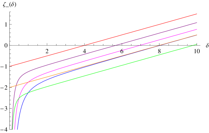
Figure 6: Level crossing of the modes $\zeta_{-}(\delta)$ from negative to positive values

D.3 The $\eta$–invariant

The results for the spectrum can been used to compute the $\eta$–invariant of the Dirac operator on Berger spheres. This invariance measures the asymmetry between the number of positive and negative modes in the spectrum, and, as such, it vanishes when $\delta=1$. This is seen by computing the $\eta$–invariant in closed form. The result is very important for evaluating the index of the Dirac operator on gravitational instanton backgrounds by the Atiyah–Patodi–Singer index theorem [19] (see also [13, 20]).

First, we examine the case $\delta<4$ which is the simplest as it does not involve level crossing. There are infinitely many positive modes $\zeta_{+}$ and $\zeta_{0}$ and infinitely many negative modes $\zeta_{-}$. Considering the difference of the spectral Riemann zeta–function between the positive and negative eigen–values, excluding zero modes,

$$\eta_{{\rm D}}(s)=\sum_{{\rm eigenvalues}}({\rm sign}~{}\zeta)~{}|\zeta|^{-s}~{},$$ (D.28)

allows to define the $\eta$–invariant of the Dirac operator by appropriate analytic continuation at $s=0$ as

$$\eta_{{\rm D}}=\eta_{{\rm D}}(0)~{}.$$ (D.29)

The $\eta$–invariant is ill–defined without the zeta–function regularization as it is the difference of two infinite numbers. Note that under rescaling of the metric the spectrum of the Dirac operator scales uniformly but $\eta_{{\rm D}}$ remains invariant since it is evaluated at $s=0$.

Then, taking into account the multiplicities of the various eigen–values, we have explicitly that

$$\eta_{{\rm D}}(s)=\sum_{p,q>0}(p+q)\Big{[}\left({\delta^{2}\over 2}+X\right)^{-s}-\left(-{\delta^{2}\over 2}+X\right)^{-s}\Big{]}+\sum_{p>0}2p\left({\delta^{2}\over 2}+p\right)^{-s}$$ (D.30)

setting

$$X=\sqrt{4\delta^{2}pq+(p-q)^{2}}$$ (D.31)

for notational convenience. The first term refers to the contribution of $\zeta_{+}$, the second to $\zeta_{-}$ and the third to $\zeta_{0}$. The first two terms are a bit tricky to evaluate, whereas the third one is more straightforward. We will present the essential tricks and details since they are also needed in the main text to evaluate more complicated sums.

The computations are most easily done by expanding all terms in power series of $\delta$. For the last one we have

$$\left({\delta^{2}\over 2}+p\right)^{-s}={1\over p^{s}}\left(1-{s\delta^{2}\over 2p}+{s(s+1)\delta^{4}\over 8p^{2}}+\cdots\right)$$ (D.32)

that yields the following expansion in terms of Riemann zeta–functions,

$$I_{0}(s)=\sum_{p>0}2p\left({\delta^{2}\over 2}+p\right)^{-s}=2\zeta(s-1)-\delta^{2}s\zeta(s)+{1\over 4}\delta^{4}s(s+1)\zeta(s+1)+\cdots~{}.$$ (D.33)

The higher order terms are irrelevant because they vanish at $s=0$ and they are omitted (they contain the factor $s\zeta(s+n)$ for all integers $n\geq 2$). Since $\zeta(-1)=-1/12$, $\zeta(0)=-1/2$ and $s\zeta(s+1)$ equals $1$ at $s=0$, we obtain immediately

$$I_{0}(0)=-{1\over 6}+{\delta^{4}\over 4}~{}.$$ (D.34)

Next, we consider the power series expansion

$$\left(\pm{\delta^{2}\over 2}+X\right)^{-s}={1\over X^{s}}\left(1\mp{s\delta^{2}\over 2X}+{s(s+1)\delta^{4}\over 8X^{2}}\mp{s(s+1)(s+2)\delta^{6}\over 48X^{3}}+\cdots\right)$$ (D.35)

that yields

$$I_{+}(s)-I_{-}(s)=\sum_{p,q>0}(p+q)\Big{[}\left({\delta^{2}\over 2}+X\right)^{-s}-\left(-{\delta^{2}\over 2}+X\right)^{-s}\Big{]}$$

$$~{}~{}~{}~{}~{}~{}~{}~{}=-\delta^{2}sf\left({s+1\over 2}\right)-{1\over 24}\delta^{6}s(s+1)(s+2)f\left({s+3\over 2}\right)+\cdots~{},$$ (D.36)

where

$$f(s)=\sum_{p,q>0}{p+q\over X^{2s}}=\sum_{p,q>0}{p+q\over[4\delta^{2}pq+(p-q)^{2}]^{s}}~{}.$$ (D.37)

The function $f(s)$ converges absolutely for ${\rm Re}s>3/2$ on the complex $s$–plane, and, therefore, the omitted terms in (D.36) are irrelevant as they vanish at $s=0$. Furthermore, the meromorphic continuation of $f(s)$ to the entire complex plane has only simple poles whose residues at $s=1/2$ and $s=3/2$ turn out to be

$${\rm res}f(s)|_{s=1/2}={\delta^{2}-1\over 6}~{},~{}~{}~{}~{}~{}~{}{\rm res}f(s)|_{s=3/2}={1\over 2\delta^{2}}~{}.$$ (D.38)

They provide the values of $(s/2)f((s+1)/2)$ and $(s/2)f((s+3)/2)$ at $s=0$. All other terms appearing in the expression (D.36) vanish at $s=0$, and, thus, we obtain

$$I_{+}(0)-I_{-}(0)={\delta^{2}\over 3}-{5\delta^{4}\over 12}~{}.$$ (D.39)

The mathematical properties of $f(s)$ can be studied using the Euler–Maclaurin summation formula that converts infinite sums into integrals – in this case of two variables (see, for instance, [99]).

There is no point in presenting the technical details of the residue formulae since they are somewhat involved. We refer the interested reader to the comprehensive report [100] for the relevant computations as well as certain generalizations to higher dimensional Berger spheres. We only note here that when $\delta=1$ the computation of the residues can be done by elementary methods. In this case $f(s)$ simplifies and it is expressed in terms of Riemann’s zeta–function as follows,

$$f(s)=\sum_{p,q>0}{1\over(p+q)^{2s-1}}=\zeta(2s-2)-\zeta(2s-1)~{}.$$ (D.41)

Then, it can be easily seen that $f(1/2)=\zeta(-1)-\zeta(0)=5/12$ is finite, and, hence, there is no pole, i.e., the residue at $s=1/2$ vanishes. Evaluating $f(3/2)=\zeta(1)-\zeta(2)$ shows that there a simple pole at $s=3/2$ given by the pole of $\zeta(2s+1)$ at $s=0$ whose residue is $1/2$ (it is convenient to compare $f(s+3/2)$ with $\zeta(2s+1)$ at $s=0$). These results agree with the general formulae (D.38) for $\delta=1$.

Finally, putting all these together, we add up the individual terms $I_{0}(0)+I_{+}(0)-I_{-}(0)$ and arrive at the following result for the $\eta$–invariant of the Dirac operator on Berger spheres with anisotropy parameter $\delta<4$, as in [39],

$$\eta_{{\rm D}}=-{1\over 6}(\delta^{2}-1)^{2}~{}.$$ (D.42)

It can be readily seen that $\eta_{{\rm D}}$ vanishes for the isotropic metric $\delta=1$, as expected. Also, in the fully squashed limit $\delta=0$, $\eta_{{\rm D}}=-1/6$ counting the asymmetry of positive and negative modes that become infinite (the finite eigen–values are equally distributed to positive and negative values).

At this point, it is instructive to compare the $\eta$–invariant with the gravitational Chern–Simons action [51]

$$W_{\rm CS}={1\over 2}\int_{\Sigma_{3}}{\rm Tr}\left(\omega\wedge d\omega+{2\over 3}\omega\wedge\omega\wedge\omega\right)$$ (D.43)

evaluated for the class of homogeneous metric on $S^{3}$. Using the Bianchi IX form of the metric (D.2) and the expressions for the connection one–forms ${\omega^{I}}_{J}$ derived earlier, we find (up to a sign convention that depends on the orientation of $S^{3}$)

$$W_{\rm CS}=16\pi^{2}\Big{[}1+{1\over 2\gamma_{1}\gamma_{2}\gamma_{3}}(\gamma_{1}+\gamma_{2}-\gamma_{3})(\gamma_{1}-\gamma_{2}+\gamma_{3})(\gamma_{1}-\gamma_{2}-\gamma_{3})\Big{]}~{}.$$ (D.44)

The result is scale invariant, as required on general grounds. Then, choosing $\gamma_{1}=\gamma_{2}=1$ and $\gamma_{3}=\delta^{2}$, we obtain immediately

$${1\over 48\pi^{2}}W_{\rm CS}({\rm Berger})={1\over 6}(\delta^{4}-2\delta^{2}+2)=-\eta_{{\rm D}}+{1\over 6}$$ (D.45)

that relates $W_{\rm CS}$ and $\eta_{{\rm D}}$ for Berger spheres. This is a special case of a more general relation among the Chern–Simons action and the $\eta$–invariant found in the context of the Atiyah–Patodi–Singer theory [19] (for a compact three–manifold without boundaries it suffices to consider a spin four–manifold bounded by it, extend the product metric near the boundary and integrate the Pontrjagin form relative to this metric).

Next, we examine the case $\delta>4$ that involves level crossing. Every time an eigenvalue $\zeta_{-}$ crosses from negative to positive values, $\eta_{{\rm D}}$ jumps by $2$ to $\eta_{{\rm D}}+2$, since the spectral asymmetry, as calculated for $\delta<4$, changes by $2$. Let us denote by

$${\cal C}(\delta_{\rm c})=\{(p,q)\in\mathbb{N}^{2};~{}~{}\delta_{\rm c}^{2}=2\sqrt{4pq\delta_{\rm c}^{2}+(p-q)^{2}}\}$$ (D.46)

the set of positive integers $(p,q)$ that account for harmonic spinors at each one of the special values $\delta_{\rm c}<\delta$. This set has at least two elements associated to the two harmonic spinors at $\delta_{\rm c}=4$. Since the zero modes at $\delta_{\rm c}$ have multiplicity $p+q$, the quantity

$$S(\delta)=\sum_{\delta_{\rm c}<\delta}\Big{[}\sum_{(p,q)\in{\cal C}(\delta_{\rm c})}(p+q)\Big{]}$$ (D.47)

provides the total number of modes that crossed from negative to positive values as $\delta$ was varying from $\delta<4$ to any given value $\delta>4$. Thus, for $\delta>4$, the $\eta$–invariant of the Dirac operator for Berger spheres is shifted by twice the number of these modes and equals

$$\eta_{{\rm D}}=-{1\over 6}(\delta^{2}-1)^{2}+2S(\delta)$$ (D.48)

provided that $\delta$ does not assume the special values (D.26).

On the other hand, if $\delta$ is tuned to any one of the values (D.26), including $\delta=4$, the corresponding zero modes have to be removed from the spectrum while computing the sum $\eta_{{\rm D}}(s)$. We also have to add $1$ for each one of these modes (i.e., shift $\eta_{{\rm D}}$ by the dimension of the space of harmonic spinors arising at those values of $\delta$), and, consequently, the net effect is zero. Thus, there is no change of $\eta_{{\rm D}}$ in this case. Changes can only occur when there is level crossing.

Summarizing, the formula (D.48) for the $\eta$–invariant is the most general one and it is valid for all values of the anisotropy parameter $\delta$ of Berger spheres. The result is finite for all finite values of $\delta$ and it only becomes infinite in the extreme limit $\delta\rightarrow\infty$ where the geometry becomes singular. In the latter case there are no negative modes left behind and the spectral asymmetry is infinite, as expected.

References

- [1] J.S. Bell and R. Jackiw, “A PCAC puzzle: in the –model", Nuovo Cimento (1969) 47.
- [2] S.L. Adler, “Axial–vector vertex in spinor electrodynamics", Phys. Rev. (1969) 2426.
- [3] R. Jackiw, “Axial anomaly", Int. J. Mod. Phys. (2010) 659.
- [4] W.A. Bardeen and A.R. White eds., Symposium on Anomalies, Geometry and Topology, World Scientific, Singapore, 1986.
- [5] K. Fujikawa, “Path–integral measure for gauge–invariant fermion theories", Phys. Rev. Lett. (1979) 1195; “Path integral for gauge theories with fermions", Phys. Rev. (1980) 2848; Erratum–ibid. (1980) 1499.
- [6] K. Fujikawa and H, Suzuki, Path Integrals and Quantum Anomalies, Oxford University Press, Oxford, 2004.
- [7] R. Delbourgo and A. Salam, “The gravitational correction to PCAC", Phys. Lett. (1972) 381.
- [8] T. Eguchi and P.G.O. Freund, “Quantum gravity and world topology", Phys. Rev. Lett. (1976) 1251.
- [9] N.K. Nielsen, H. Römer and B. Schroer, “Classical anomalies and local version of the Atiyah–Singer theorem", Phys. Lett. (1977) 445; “Anomalous currents in curved space", Nucl. Phys. (1978) 475.
- [10] L. Alvarez–Gaumé and E. Witten, “Gravitational anomalies", Nucl. Phys. (1983) 269.
- [11] G. ’t Hooft, “Symmetry breaking through Bell–Jackiw anomalies", Phys. Rev. Lett. (1976) 8; “Computation of the quantum effects due to a four–dimensional pseudoparticle", Phys. Rev. (1976) 3432; Erratum–ibid. (1978) 2199.
- [12] M.F. Ayiyah and I.M. Singer, “Index of elliptic operators", Ann. Math. (1968) 485; ibid. (1968) 531; ibid. (1968) 546; ibid. (1971) 119; ibid. (1971) 139.
- [13] P.B. Gilkey, Invariance Theory, the Heat Equation, and the Atiyah–Singer Index Theorem, Studies in Advanced Mathematics, second edition, CRC Press, Boca Raton, 1995.
- [14] N. Berline, E. Getzler and M. Vergne, Heat Kernels and Dirac Operators, Springer–Verlag, Berlin, 2004.
- [15] N. Hitchin, “Compact four–dimensional Einstein manifolds", J. Diff. Geom. (1974) 435.
- [16] S.T. Yau, “On Calabi’s conjecture and some new results on algebraic geometry", Proc. Nat. Acad. Sci. USA (1977) 1798.
- [17] A. Lichnerowicz, “Spineurs harmoniques", C.R. Acad. Sci. (1963) 7.
- [18] G.W. Gibbons and C.N. Pope, “The positive action conjecture and asymptotically Euclidean metrics in quantum gravity", Commun. Math. Phys. (1979) 267.
- [19] M.F. Atiyah, V.K. Patodi and I.M. Singer, “Spectral asymmetry and Riemannian geometry", Proc. Camb. Philos. Soc. (1975) 43; ibid. (1975) 405; ibid. (1976) 71.
- [20] R. Melrose, The Atiyah–Padoti–Singer Index Theorem, A.K. Peters Ltd, Wellesley, 1993.
- [21] S.W. Hawking, “Gravitational instantons", Phys. Lett. (1977) 81.
- [22] T. Eguchi and A.J. Hanson, “Asymptotically flat self–dual solutions to Euclidean gravity", Phys. Lett. (1978) 249.
- [23] H. Römer and B. Schroer, “Fractional winding numbers and surface effects", Phys. Lett. (1977) 182.
- [24] T. Eguchi, P.B. Gilkey and A.J. Hanson, “Topological invariants and absence of an axial anomaly for a Euclidean Taub–NUT (Newman–Unti–Tamburino) metric", Phys. Rev. (1978) 423.
- [25] C.N. Pope, “Axial–vector anomalies and the index theorem in charged Schwarzschild and Taub–NUT spaces", Nucl. Phys. (1978) 432.
- [26] G.W. Gibbons, C.N. Pope and H. Römer, “Index theorem boundary terms for gravitational instantons", Nucl. Phys. (1979) 377.
- [27] S.W. Hawking and C.N. Pope, “Symmetry breaking by instantons in supergravity", Nucl. Phys. (1978) 381.
- [28] A.J. Hanson and H. Römer, “Gravitational instanton contribution to spin axial anomaly", Phys. Lett. (1978) 58.
- [29] T. Eguchi, P.B. Gilkey and A.J. Hanson, “Gravitation, gauge theories and differential geometry", Phys. Rept. (1980) 213.
- [30] P. Hořava, “Membranes at quantum criticality", JHEP (2009) 020 [arXiv:0812.4287[hep–th]].
- [31] P. Hořava, “Quantum gravity at a Lifshitz point", Phys. Rev. (2009) 084008 [arXiv:0901.3775[hep–th]].
- [32] D. Blas, O. Pujolas and S. Sibiryakov, “Models of non–relativistic quantum gravity: The good, the bad and the healthy", preprint [arXiv:1007.3503 [hep–th]].
- [33] T. Sotiriou, “Hořava–Lifshitz gravity: a status report", J. Phys. Conf. Ser. (2011) 012034 [arXiv:1010.3218[hep–th]].
- [34] M. Henneaux, A. Kleinschmidt and G. Lucena Gomez, “A dynamical inconsistency of Hořava gravity", Phys. Rev. (2010) 064002 [arXiv:0912.0399[hep–th]].
- [35] P. Hořava and C.M. Melby–Thompson, “General covariance in quantum gravity at a Lifshitz point", Phys. Rev. (2010) 064027 [arXiv:1007.2410[hep–th]]; P. Hořava, “General covariance in gravity at a Lifshitz point", preprint [arXiv:1101.1081[hep–th]].
- [36] A. Dhar, G. Mandal and S.R. Wadia, “Asymptotically free four–fermi theory in 4 dimensions at the Lifshitz–like fixed point", Phys. Rev. (2009) 105018 [arXiv:0905.2928[hep–th]].
- [37] P. Hořava, “Quantum criticality and Yang–Mills gauge theory", Phys. Lett. (2010) 172 [arXiv:0811.2217[hep–th]].
- [38] I. Bakas, F. Bourliot, D. Lüst and M. Petropoulos, “Geometric flows in Hořava–Lifshitz gravity", JHEP (2010) 131 [arXiv:1002.0062[hep–th]]; I. Bakas, “Gradient flows and instantons at a Lifshitz point", J. Phys. Conf. Ser. (2011) 012004 [arXiv:1009.6173[hep–th]].
- [39] N.J. Hitchin, “Harmonic spinors", Adv. Math. (1974) 1.
- [40] C. Bär, “The Dirac operator on homogeneous spaces and its spectrum on 3–dimensional lens spaces", Arch. Math. (1992) 65; “Metrics with harmonic spinors", Geom. Funct. Anal. (1996) 899.
- [41] B.S. DeWitt, “Dynamical Theory of Groups and Fields" in Relativity, Groups and Topology, eds. C. DeWitt and B. DeWitt, Gordon and Breach, New York, 1965; “Quantum theory of gravity. III. Applications of the covariant theory", Phys. Rev. (1967) 1239.
- [42] J.L. Synge, Relativity: The General Theory, North Holland, Amsterdam, 1960.
- [43] J. Hadamard, Lectures on Cauchy’s Problem in Linear Partial Differential Equations, Yale University Press, New Haven, 1923.
- [44] C.W. Misner, K.S. Thorne and J.A. Wheeler, Gravitation, Freeman, San Francisco, 1973.
- [45] C.R. Hagen, “Scale and conformal transformations in Galilean–covariant field theory", Phys. Rev. (1972) 377.
- [46] J. Schwinger, “On gauge invariance and vacuum polarization", Phys. Rev. (1951) 664.
- [47] C. Itzykson and J.–B. Zuber, Quantum Field Theory, McGraw–Hill, New York, 1980.
- [48] W. Xue, “Non–relativistic supersymmetry", preprint [arXiv:1008.5102[hep–th]].
- [49] B.S. DeWitt, “Quantum theory of gravity. I. The canonical theory", Phys. Rev. (1967) 1113.
- [50] S. Deser, R. Jackiw and S. Templeton, “Three-Dimensional Massive Gauge Theories", Phys. Rev. Lett. (1982) 975; “Topologically massive gauge theories", Annals Phys. (1982) 372; Erratum–ibid. (1988) 406.
- [51] S.S. Chern and J. Simons, “Characteristic forms and geometric invariants", Ann. Math. (1974) 48.
- [52] J.H. Horne and E. Witten, “Conformal gravity in three dimensions as a gauge theory", Phys. Rev. Lett. (1989) 501.
- [53] H.D. Cao, B. Chow, S.–C. Chu and S.–T. Yau eds., Collected Papers on Ricci Flow, Series in Geometry and Physics, International Press, Somerville, 2003.
- [54] P. Topping, Lectures on the Ricci Flow, London Mathematical Society Lecture Note Series, Cambridge University Press, Cambridge, 2006.
- [55] B. Chow, P. Lu and L. Ni, Hamilton’s Ricci Flow, Graduate Texts in Mathematics, American Mathematical Society, Science Press, Providence, 2006.
- [56] A.U.O. Kisisel, O. Sarioglu and B. Tekin, “Cotton flow", Class. Quant. Grav. (2008) 165019 [arXiv:0803.1603[hep–th]].
- [57] M.–I. Park, “Hořava gravity and gravitons at a conformal point", preprint [arXiv:0910.5117[hep–th]].
- [58] R. Jackiw, “A nonrelativistic chiral soliton in one dimension", J. Nonlin. Math. Phys. (1997) 261 [arXiv:hep–th/9611185].
- [59] L. Griguolo and D. Seminara, “Chiral solitons from dimensional reduction of Chern–Simons gauged non–linear Schrödinger equation: classical and quantum aspects", Nucl. Phys. (1998) 467 [arXiv:hep–th/9709075].
- [60] C.W. Misner, “Mixmaster universe", Phys. Rev. Lett. (1969) 1071; “Quantum cosmology 1", Phys. Rev. (1969) 1319.
- [61] I. Bakas, F. Bourliot, D. Lüst and M. Petropoulos, “Mixmaster universe in Hořava–Lifshitz gravity", Class. Quant. Grav. (2010) 045013 [arXiv:0911.2665 [hep-th]].
- [62] J. Isenberg and M. Jackson, “Ricci flow of locally homogeneous geometries on closed manifolds", J. Diff. Geom. (1992) 723.
- [63] R. Jackiw, “Quantum meaning of classical field theory", Rev. Mod. Phys. (1977) 681.
- [64] R. Rajaraman, Solitons and Instantons, North Holland, Amsterdam, 1987.
- [65] C. Callias, “Axial anomalies and index theorems on open spaces", Commun. Math. Phys. (1978) 213; R. Bott and R. Seeley, “Some remarks on the paper of Callias", Commun. Math. Phys. (1978) 235.
- [66] V. Rubakov, Classical Theory of Gauge Fields, Princeton University Press, Princeton, 2002.
- [67] G. Calcagni, “Cosmology of the Lifshitz universe", JHEP (2009) 112 [arXiv:0904.0829[hep–th]].
- [68] E. Kiritsis and G. Kofinas, “Hořava–Lifshitz cosmology", Nucl. Phys. (2009) 467 [arXiv:0904.1334[hep–th]].
- [69] R. Brandenberger, “Matter bounce in Hořava–Lifshitz cosmology", Phys. Rev. (2009) 043516 [arXiv:0904.2835[hep–th]].
- [70] R. Percacci and E. Sezgin, “One loop beta functions in topologically massive gravity", Class. Quant. Grav. (2010) 155009 [arXiv:1002.2640[hep–th]].
- [71] N.J. Hitchin, “Einstein metrics and the eta–invariant", Bolletino U.M.I. (7) Suppl. Fasc. 2 (1997) 95.
- [72] G.W. Gibbons and S.W. Hawking, “Action integrals and partition functions in quantum gravity", Phys. Rev. (1977) 2752.
- [73] J. York, “Role of conformal three–geometry in the dynamics of gravitation", Phys. Rev. Lett. (1972) 1082.
- [74] I.I. Cotaescu, S. Moroianu and M. Visinescu, “Quantum anomalies for generalized Euclidean Taub–NUT metrics", J. Phys. (2005) 7005; S. Moroianu and M. Visinescu, “–index of the Dirac operator of generalized Euclidean Taub–NUT metrics", preprint [arXiv:math–ph/0511025].
- [75] A. Moroianu and S. Moroianu, “The Dirac operator on generalized Taub–NUT spaces", preprint [arXiv:1003.5364[math.DG]].
- [76] S.M. Christensen and M.J. Duff, “Axial and conformal anomalies for arbitrary spin in gravity and supergravity", Phys. Lett. (1978) 571; “New gravitational index theorems and super theorems", Nucl. Phys. (1979) 301.
- [77] M.T. Grisaru, H. Römer, N.K. Nielsen and P. van Nieuwenhuisen, “Approaches to the gravitational spin– axial anomaly", Nucl. Phys. (1978) 477.
- [78] M.J. Perry, “Anomalies in supergravity", Nucl. Phys. (1978) 114.
- [79] H. Römer, “Axial anomaly and boundary terms for spinor fields", Phys. Lett. (1979) 172.
- [80] A.N. Redlich, “Parity violation and gauge non–invariance of the effective gauge field action in three dimensions", Phys. Rev. (1984) 2366.
- [81] I. Vuorio, “Parity violation and the effective gravitational action in three dimensions", Phys. Lett. (1986) 176.
- [82] L. Alvarez–Gaumé, S. Della Pietra and G. Moore, “Anomalies and odd dimensions", Annals Phys. (1985) 288.
- [83] R.S. Hamilton, “Three manifolds of positive Ricci curvature", J. Diff. Geom. (1982) 255.
- [84] J. Milnor, “Towards the Poincaré conjecture and the classification of –manifolds", Notices of Amer. Math. Soc. (2003) 1226; M.T. Anderson, “Geometrization of –manifolds via the Ricci flow", Notices of Amer. Math. Soc. (2004) 184.
- [85] N. Hitchin, “Polygons and gravitons", Math. Proc. Camb. Phil. Soc. (1979) 465.
- [86] P.B. Kronheimer, “The construction of ALE spaces as hyper–Kähler quotients", J. Diff. Geom. (1989) 665.
- [87] S. Goette, “Computations and applications of invariants", preprint [arXiv:1011.4766[math.DG]].
- [88] J.L. Friedman and R. Sorkin, “Spin from gravity", Phys. Rev. Lett. (1980) 1100.
- [89] J.L. Friedman and D.M. Witt, “Internal symmetry groups of quantum geons", Phys. Lett. (1983) 324.
- [90] T. Regge and C. Teitelboim, “Role of surface integrals in the Hamiltonian formulation of general relativity", Annals Phys. (1974) 286.
- [91] S.W. Hawking and G.T. Horowitz, “The gravitational Hamiltonian, action, entropy and surface terms", Class. Quant. Grav. (1996) 1487 [arXiv:gr–qc/9501014].
- [92] M.J. Duff, “Twenty years of the Weyl anomaly", Class. Quant. Grav. (1994) 1387 [arXiv:hep–th/9308075].
- [93] I. Adam, I.V. Melnikov and S. Theisen, “A non–relativistic Weyl anomaly", JHEP (2009) 130 [arXiv:0907.2156[hep–th]].
- [94] A. Davody, “Weyl anomaly in non–relativistic CFTs", Phys. Lett. (2010) 341 [arXiv:0909.3705[hep–th]].
- [95] R. Jackiw and J.R. Schrieffer, “Solitons with fermion number in condensed matter and relativistic field theories", Nucl. Phys. [FS3] (1981) 253.
- [96] R. Jackiw and S.–Y. Pi, “Chiral gauge theory for graphene", Phys. Rev. Lett. (2007) 266402 [arXiv:cond–mat/0701760].
- [97] S.A. Fulling, Aspects of Quantum Field Theory in Curved Space–Time, Cambridge University Press, Cambridge, 1989.
- [98] M. Carmeli, Group Theory and General Relativity, McGraw–Hill, New York, 1977.
- [99] G. Tenenbaum, Introduction to Analytic and Probabilistic Number Theory, Cambridge University Press, Cambridge, 1996.
- [100] M Habel and M. Peter, “The eta invariant of Berger spheres and hypergeometric identities", preprint, Mathematisches Institut, Albert–Ludwigs–Universität, 2002.