Two-state Bose-Hubbard model
in the hard-core boson limit

Abstract

Phase transition into the phase with Bose-Einstein (BE) condensate in the two-band Bose-Hubbard model with the particle hopping in the excited band only is investigated. Instability connected with such a transition (which appears at excitation energies $\delta<\lvert t_{0}^{\prime}\rvert$, where $\lvert t_{0}^{\prime}\rvert$ is the particle hopping parameter) is considered. The re-entrant behaviour of spinodales is revealed in the hard-core boson limit in the region of positive values of chemical potential. It is found that the order of the phase transition undergoes a change in this case and becomes the first one; the re-entrant transition into the normal phase does not take place in reality. First order phase transitions also exist at negative values of $\delta$ (under the condition $\delta>\delta_{\mathrm{crit}}\approx-0.12\lvert t_{0}^{\prime}\rvert$). At $\mu<0$ the phase transition mostly remains to be of the second order. The behaviour of the BE-condensate order parameter is analyzed, the $(\Theta,\mu)$ and $(\lvert t_{0}^{\prime}\rvert,\mu)$ phase diagrams are built and localizations of tricritical points are established. The conditions are found at which the separation on the normal phase and the phase with the BE condensate takes place.

Key words: Bose-Hubbard model, hard-core bosons, Bose-Einstein condensation, excited band

PACS: 03.75.Hh, 03.75.Lm, 64.70.Tg, 71.35.Lk, 37.10.Jk, 67.85.-d

1 Introduction

During the recent years Bose-Hubbard model (BHM) is proved to be a valuable tool in the theory of systems of strongly correlated particles. The model achieves a wide recognition due to a successful description of thermodynamics and dynamics of ultracold Bose atoms in optical lattices where a phase transition to the phase with the Bose-Einstein (BE) condensate (so-called Mott insulator (MI) – superfluid state (SF) transition) occurs at very low temperatures. Experimental evidence of BE condensation in optical lattices was found for the first time in works [1, 2] while theoretical predictions of such an effect were given earlier [3]. Starting from the 90-ies of the past century, a series of papers were devoted to the theory of this phenomenon. Among the first key articles on the subject one should mention the work [4] where BHM was studied in the mean field approximation. The calculated therein phase diagrams demonstrate that in the simplest case (i.e., hopping of Bose particles in the presence of a single-site Hubbard repulsion) the MI-SF transition is of the second order. Moreover, it is supposed that particles reside in the ground state of local potential wells in the lattice. Forthcoming theoretical investigations in this field were performed with the use of various techniques, e.g., the random phase approximation (RPA) in the Green function method [5, 6], a strong-coupling perturbation theory [7, 8], the dynamical mean field theory (Bose-DMFT) [9, 10] as well as quantum Monte-Carlo calculations [11, 12] and other numerical methods.

The Bose-Hubbard model is also intensively used for a theoretical description of a wide range of phenomena: quantum delocalization of hydrogen atoms adsorbed on the surface of transition metals [13, 14], quantum diffusion of light particles on the surface or in the bulk [15, 16], thermodynamics of the impurity ion intercalation into semiconductors [17, 18].

In the last mentioned applications, there is usually a restriction on the position occupation number ($n_{i}\leqslant 1$), which corresponds to the limit of an infinite Hubbard repulsion for the considered model. Such a model of hard-core ions (where particles are described by the Pauli statistics) is also known as the fundamental one for the investigation of a wide range of problems, e.g., superconductivity due to a local electron pairing [19] or ionic hopping in ionic (superionic) conductors [20, 21].

The study of a quantum delocalization or diffusion reveals an important role of excited vibrational states of particles (ions) in localized (interstitial) positions with a much higher probability of ion hopping between them [15, 22, 23]. A similar issue of a possible BE condensation in the excited bands in optical lattices is also considered but the condition of their sufficient occupation due to the optical pumping (see, e.g. [24]) is imposed. An orbital degeneration of the excited $p$-state is accompanied by anisotropy of hopping parameters and causes the appearance of variously polarized bands in the one-particle spectrum. Such bands correspond by convention to different sorts (so-called ‘‘flavours’’) of bosons and their number correlates with the lattice dimensionality. In the framework of the necessary generalization of the Bose-Hubbard model, a possibility of the MI-SF transition to the phase with BE condensate in the pumping-induced quasi-equilibrium long-living state of the system has been established [25].

In the equilibrium case, the issue of BE condensation involving the excited states in the framework of ordinary Bose-Hubbard model was not considered in practice. The exception is the system of spin-1 bosons [26, 27] where a hyperfine splitting gives rise to multiplets of local states resulting in closely-spaced excited levels. As demonstrated in [28, 29], the MI-SF phase transition could be of the first order when a single-site spin interaction is of the ‘‘antiferromagnetic’’ type. A similar change of the phase transition order also takes place for multicomponent Bose systems in the optical lattices [30].

In the present work we consider an equilibrium thermodynamics of the Bose-Hubbard model taking into account only one nondegenerated excited state on the lattice site besides the ground one. On the one hand, such a model corresponds to 1D or strongly anisotropic (quasi-1D) optical lattice, and on the other hand, it is close to a situation that is characteristic of a system of light particles adsorbed on the metal surface. For example, the excited states of hydrogen atoms on the Ni(111) surface are sufficiently distant [22] so only the lowest one could be taken into account. We shall investigate a condition of instability of a normal state of the Bose system with respect to BE condensation considering a criterion of divergence of the susceptibility ($\chi\sim\langle\langle c_{l}|c_{p}^{+}\rangle\rangle_{\omega}|_{q=0,\omega=0}$) characterizing the system response with respect to the field related to a spontaneous creation or annihilation of particles. We shall also study the behaviour of the order parameter $\langle c_{0}\rangle$ ($\langle c_{0}^{+}\rangle$) as well as the grand canonical potential in the region of the MI-SF transition and shall build relevant phase diagrams. Special attention will be paid to a change of the phase transition order and localization of tricritical points at different values of excitation energy, particle hopping parameter and temperature.

We shall limit ourselves to the hard-core boson (HCB) limit where a limitation on occupation numbers is present: no more than one particle per site regardless of the state (excited or ground) occupied by it. Thus, the single-site problem is a three-level one (contrary to the two-level ordinary HCB case). For this reason, it is convenient to use the formalism of Hubbard operators [31] (standard basis operators [32]).

2 Two-state Bose-Hubbard model in RPA: normal phase

The Bose-Hubbard model is used for description of the system of Bose particles which are located in a periodic field and can reside in lattice sites. Taking into account only the ground and the first excited vibrational levels in the potential well on the site, one can express the model Hamiltonian as:

$$\hat{H} =(\varepsilon-\mu)\sum_{i}b_{i}^{+}b_{i}+(\varepsilon^{\prime}-\mu)\sum_{i}c_{i}^{+}c_{i}+\frac{U_{b}}{2}\sum_{i}n_{i}^{b}(n_{i}^{b}-1)+\frac{U_{c}}{2}\sum_{i}n_{i}^{c}(n_{i}^{c}-1)+U_{bc}\sum_{i}n_{i}^{b}n_{i}^{c}$$

$$\quad+\sum_{ij}t_{ij}^{b}b_{i}^{+}b_{j}+\sum_{ij}t_{ij}^{c}c_{i}^{+}c_{j}+\sum_{ij}t_{ij}^{bc}(b_{i}^{+}c_{j}+c_{i}^{+}b_{j}),$$ (2.1)

where $b_{i}$ and $b_{i}^{+}$ ($c_{i}$ and $c_{i}^{+}$) are Bose operators of annihilation and creation of particles in the ground (excited) state, $\varepsilon$ and $\varepsilon^{\prime}$ are respective energies of state and $\mu$ is the chemical potential of particles. Such a Hamiltonian includes the single-site Hubbard repulsions with energies $U_{b}$, $U_{c}$ and $U_{bc}$ as well as the particle hopping between ground ($t^{b}$), excited ($t^{c}$) and different ($t^{bc}$) states. Hereinafter we assume $U_{b}=U_{c}=U_{bc}$ for simplicity.

Let us define a single-site basis $|n_{i}^{b},n_{i}^{c}\rangle\equiv|i;n_{i}^{b},n_{i}^{c}\rangle$ (which is formed by particle occupation numbers in the ground and in the excited states, i.e., eigenvalues of operators $n_{i}^{b}=b_{i}^{+}b_{i}$ and $n_{i}^{c}=c_{i}^{+}c_{i}$) as well as introduce Hubbard operators (standard basis operators)

$$X_{i}^{n,m;n^{\prime},m^{\prime}}\equiv|i;n,m\rangle\langle i;n^{\prime},m^{\prime}|.$$ (2.2)

Annihilation and creation Bose operators may be written as

$$b_{i} =\sum_{n}\sum_{m}\sqrt{n+1}\,X_{i}^{n,m;n+1,m}, b_{i}^{+} =\sum_{n}\sum_{m}\sqrt{n+1}\,X_{i}^{n+1,m;n,m};$$

$$c_{i} =\sum_{n}\sum_{m}\sqrt{m+1}\,X_{i}^{n,m;n,m+1}, c_{i}^{+} =\sum_{n}\sum_{m}\sqrt{m+1}\,X_{i}^{n,m+1;n,m}.$$ (2.3)

Corresponding occupation numbers look as follows

$$n_{i}^{b} =\sum_{n}\sum_{m}nX_{i}^{n,m;n,m}, n_{i}^{c} =\sum_{n}\sum_{m}mX_{i}^{n,m;n,m},$$ (2.4)

where summation indices $n,m=0,\dotsc,\infty$ in both (2.3) and (2.4) formulae.

In the $X$-operator representation, the single-site part of Hamiltonian (2.1) can be written as

$$\hat{H}_{0} =\sum_{i}\sum_{n}\sum_{m}\lambda_{nm}X_{i}^{n,m;n,m},$$ (2.5)

where

$$\lambda_{nm} =n(\varepsilon-\mu)+m(\varepsilon^{\prime}-\mu)+\frac{U}{2}(n+m)(n+m-1).$$ (2.6)

Terms describing an inter-site transfer in Hamiltonian (2.1) are transformed in a similar way.

Our primary goal is to calculate the two-time temperature boson Green’s functions $\langle\langle b|b^{+}\rangle\rangle$ and $\langle\langle c|c^{+}\rangle\rangle$, which describe an excitation spectrum and make it possible to investigate the conditions of the system’s instability with respect to the spontaneous symmetry breaking and the appearance of a BE condensate. As follows from definitions (2.3)

$$\langle\langle b_{l}|b_{p}^{+}\rangle\rangle_{\omega} =\sum_{nm}\sum_{rs}\sqrt{n+1}\,\sqrt{r+1}\,\langle\langle X_{l}^{n,m;n+1,m}|X_{p}^{r+1,s;r,s}\rangle\rangle_{\omega}\,,$$

$$\langle\langle c_{l}|c_{p}^{+}\rangle\rangle_{\omega} =\sum_{nm}\sum_{rs}\sqrt{m+1}\,\sqrt{s+1}\,\langle\langle X_{l}^{n,m;n,m+1}|X_{p}^{r,s+1;r,s}\rangle\rangle_{\omega}\,.$$ (2.7)

We will use the equation-of-motion method for the evaluation of $X$-operator Green’s functions. For the first one, from relations (2.7) one could write

$$\hbar\omega\langle\langle X_{l}^{n,m;n+1,m}|X_{p}^{r+1,s;r,s}\rangle\rangle_{\omega} =\frac{\hbar}{2\pi}\langle X_{l}^{n,m;n,m}-X_{l}^{n+1,m;n+1,m}\rangle\delta_{lp}\delta_{nr}\delta_{ms}$$

$$\quad+\langle\langle[X_{l}^{n,m;n+1,m},\hat{H}]|X_{p}^{r+1,s;r,s}\rangle\rangle_{\omega}\,.$$ (2.8)

Let us write the commutators

$$[X_{l}^{n,m;n+1,m},\hat{H}_{0}] =(\lambda_{n+1,m}-\lambda_{n,m})X_{l}^{n,m;n+1,m},$$ (2.9)

$$[X_{l}^{n,m;n+1,m},b_{i}^{+}] =\delta_{li}\sqrt{n+1}\left(X_{l}^{n,m;n,m}-X_{l}^{n+1,m;n+1,m}\right),$$ (2.10a)

$$[X_{l}^{n,m;n+1,m},b_{i}] =\delta_{li}\left(\sqrt{n+2}\,X_{l}^{n,m;n+2,m}-\sqrt{n}\,X_{l}^{n-1,m;n+1,m}\right),$$ (2.10b)

$$[X_{l}^{n,m;n+1,m},c_{i}^{+}] =\delta_{li}\left(\sqrt{m}\,X_{l}^{n,m;n+1,m-1}-\sqrt{m+1}\,X_{l}^{n,m+1;n+1,m}\right),$$ (2.10c)

$$[X_{l}^{n,m;n+1,m},c_{i}] =\delta_{li}\left(\sqrt{m+1}\,X_{l}^{n,m;n+1,m+1}-\sqrt{m}\,X_{l}^{n,m-1;n+1,m}\right).$$ (2.10d)

The latter are originated from the commutation of an initial $X$-operator with the inter-site transfer terms of the Hamiltonian, thus producing the higher-order Green’s functions

$$\langle\langle X_{l}^{\dotsm}b_{j}|X_{p}^{r+1,s;r,s}\rangle\rangle_{\omega}\,,\quad\langle\langle X_{l}^{\dotsm}b_{j}^{+}|X_{p}^{r+1,s;r,s}\rangle\rangle_{\omega}\,,\dotsc,$$ (2.11)

where $X_{l}^{\dotsm}$ stands for operators on the right-hand side of expressions (2.10a)–(2.10d).

Decoupling of functions (2.11) in the random phase approximation (RPA) is performed in the following way:

$$\langle\langle X_{l}^{\dotsm}b_{j}|X_{p}^{r+1,s;r,s}\rangle\rangle_{\omega}\approx\langle X_{l}^{\dotsm}\rangle\langle\langle b_{j}|X_{p}^{r+1,s;r,s}\rangle\rangle_{\omega}+\langle b_{j}\rangle\langle\langle X_{l}^{\dotsm}|X_{p}^{r+1,s;r,s}\rangle\rangle_{\omega}\,.$$ (2.12)

In the case of the normal phase (which will be studied herein) $\langle b_{j}\rangle=\langle b_{j}^{+}\rangle=0$. Thus, retaining only the averages $\langle X_{l}^{\dotsm}\rangle$ of diagonal $X$-operators we have

$$[X_{l}^{n,m;n+1,m},\hat{H}]\approx\Delta_{nm}X_{l}^{n,m;n+1,m}+\sqrt{n+1}\,Q_{nm}\sum_{j}t_{lj}b_{j}+\sqrt{n+1}\,Q_{nm}\sum_{j}t_{lj}^{\prime\prime}c_{j}$$ (2.13)

and equation (2.8) can be rewritten as

$$\langle\langle X_{l}^{n,m;n+1,m}|X_{p}^{r+1,s;r,s}\rangle\rangle_{\omega}=\frac{\hbar}{2\pi}\delta_{lp}\delta_{nr}\delta_{ms}\frac{Q_{nm}}{\hbar\omega-\Delta_{nm}}\\ +\frac{\sqrt{n+1}\,Q_{nm}}{\hbar\omega-\Delta_{nm}}\sum_{j}t_{lj}\langle\langle b_{j}|X_{p}^{r+1,s;r,s}\rangle\rangle_{\omega}+\frac{\sqrt{n+1}\,Q_{nm}}{\hbar\omega-\Delta_{nm}}\sum_{j}t_{lj}^{\prime\prime}\langle\langle c_{j}|X_{p}^{r+1,s;r,s}\rangle\rangle_{\omega}\,.$$ (2.14)

The following notations are introduced

$$Q_{nm}=\langle X_{l}^{n,m;n,m}-X_{l}^{n+1,m;n+1,m}\rangle,\qquad\Delta_{nm}=\lambda_{n+1,m}-\lambda_{n,m}\,,$$ (2.15)

for the occupation difference of adjacent levels and the related transition energies when the number of Bose particles in the ground state (with the energy $\varepsilon$) on the site increases by one.

Proceeding from $X$-operators in equation (2.14) to the Bose operators $b$ and $b^{+}$ according to definition (2.3) we obtain

$$\langle\langle b_{l}|b_{p}^{+}\rangle\rangle_{\omega}=\frac{\hbar}{2\pi}\delta_{lp}g_{0}(\omega)+g_{0}(\omega)\biggl{(}\sum_{j}t_{lj}\langle\langle b_{j}|b_{p}^{+}\rangle\rangle_{\omega}+\sum_{j}t_{lj}^{\prime\prime}\langle\langle c_{j}|b_{p}^{+}\rangle\rangle_{\omega}\biggr{)},$$ (2.16)

where the function

$$g_{0}(\omega)=\sum_{nm}\frac{Q_{nm}}{\hbar\omega-\Delta_{nm}}(n+1)$$ (2.17)

has the meaning of the unperturbed Green’s function for bosons residing in the single-site ground state.

Equations of motion for ‘‘mixed’’ Green’s functions $\langle\langle c|b^{+}\rangle\rangle$ are obtained in the way similar to the above described scheme. Using decoupling (2.12) one can write

$$[X_{l}^{n,m;n,m+1},\hat{H}]\approx\Delta_{nm}^{\prime}X_{l}^{n,m;n,m+1}+\sqrt{m+1}\,Q_{nm}^{\prime}\sum_{j}t_{lj}^{\prime\prime}b_{j}+\sqrt{m+1}\,Q_{nm}^{\prime}\sum_{j}t_{lj}^{\prime}c_{j}\,,$$ (2.18)

which results in the equation

$$\langle\langle c_{l}|b_{p}^{+}\rangle\rangle_{\omega}=g_{0}^{\prime}(\omega)\biggl{(}\sum_{j}t_{lj}^{\prime\prime}\langle\langle b_{j}|b_{p}^{+}\rangle\rangle_{\omega}+\sum_{j}t_{lj}^{\prime}\langle\langle c_{j}|b_{p}^{+}\rangle\rangle_{\omega}\biggr{)}.$$ (2.19)

Here, similarly to (2.15) and (2.17)

$$Q_{nm}^{\prime}=\langle X_{l}^{n,m;n,m}-X_{l}^{n,m+1;n,m+1}\rangle,\quad\Delta_{nm}^{\prime}=\lambda_{n,m+1}-\lambda_{n,m}\,,\quad g_{0}^{\prime}(\omega)=\sum_{nm}\frac{Q_{nm}^{\prime}}{\hbar\omega-\Delta_{nm}^{\prime}}(m+1),$$ (2.20)

and the function $g_{0}^{\prime}(\omega)$ is the unperturbed Green’s function for bosons residing in the excited state.

By means of the Fourier transform

$$\langle\langle b_{l}|b_{p}^{+}\rangle\rangle_{\omega}=\frac{1}{N}\sum_{q}\mathrm{e}^{\mathrm{i}\mathbf{q}(\mathbf{R}_{l}-\mathbf{R}_{p})}\langle\langle b|b^{+}\rangle\rangle_{q,\omega}\,,$$ (2.21)

one can proceed to the momentum representation obtaining a system of equations

$$\langle\langle b|b^{+}\rangle\rangle_{q,\omega} =\frac{\hbar}{2\pi}g_{0}(\omega)+g_{0}(\omega)t_{q}\langle\langle b|b^{+}\rangle\rangle_{q,\omega}+g_{0}(\omega)t_{q}^{\prime\prime}\langle\langle c|b^{+}\rangle\rangle_{q,\omega}\,,$$

$$\langle\langle c|b^{+}\rangle\rangle_{q,\omega} =g_{0}^{\prime}(\omega)t_{q}^{\prime\prime}\langle\langle b|b^{+}\rangle\rangle_{q,\omega}+g_{0}^{\prime}(\omega)t_{q}^{\prime}\langle\langle c|b^{+}\rangle\rangle_{q,\omega}\,,$$ (2.22)

where $t_{q}$ , $t_{q}^{\prime}$ and $t_{q}^{\prime\prime}$ stand for the Fourier transforms of hopping parameters.

A pair of equations for other Green’s functions are obtained in a similar way

$$\langle\langle b|c^{+}\rangle\rangle_{q,\omega} =g_{0}(\omega)t_{q}\langle\langle b|c^{+}\rangle\rangle_{q,\omega}+g_{0}(\omega)t_{q}^{\prime\prime}\langle\langle c|c^{+}\rangle\rangle_{q,\omega}\,,$$

$$\langle\langle c|c^{+}\rangle\rangle_{q,\omega} =\frac{\hbar}{2\pi}g_{0}^{\prime}(\omega)+g_{0}^{\prime}(\omega)t_{q}^{\prime\prime}\langle\langle b|c^{+}\rangle\rangle_{q,\omega}+g_{0}^{\prime}(\omega)t_{q}^{\prime}\langle\langle c|c^{+}\rangle\rangle_{q,\omega}\,.$$ (2.23)

Solutions of equations (2.22) and (2.23) are as follows:

$$\langle\langle b|b^{+}\rangle\rangle_{q,\omega} =\frac{\hbar}{2\pi}\frac{1}{D_{q}(\omega)}g_{0}(\omega)(1-g_{0}^{\prime}(\omega)t_{q}^{\prime}),$$

$$\langle\langle c|c^{+}\rangle\rangle_{q,\omega} =\frac{\hbar}{2\pi}\frac{1}{D_{q}(\omega)}g_{0}^{\prime}(\omega)(1-g_{0}^{\prime}(\omega)t_{q}),$$

$$\langle\langle c|b^{+}\rangle\rangle_{q,\omega} =\frac{\hbar}{2\pi}\frac{1}{D_{q}(\omega)}g_{0}(\omega)g_{0}^{\prime}(\omega)t_{q}^{\prime\prime}=\langle\langle b|c^{+}\rangle\rangle_{q,\omega}\,,$$ (2.24)

where

$$D_{q}(\omega)=1-g_{0}(\omega)t_{q}-g_{0}^{\prime}(\omega)t_{q}^{\prime}+g_{0}(\omega)g_{0}^{\prime}(\omega)\left[t_{q}t_{q}^{\prime}-(t_{q}^{\prime\prime})^{2}\right].$$ (2.25)

The equation $D_{q}(\omega)=0$ gives the excitation spectrum which is obtained here in the RPA. On the other hand, the divergence of boson Green’s functions (2.24) at the zero values of wave vector and frequency is the criterion of instability with respect to BE condensation [5, 33], thus giving the following condition

$$D_{q=0}(\omega=0)=0,$$ (2.26)

which can be rewritten in the explicit form

$$1-g_{0}(\omega)t_{q}-g_{0}^{\prime}(\omega)t_{q}^{\prime}+g_{0}(\omega)g_{0}^{\prime}(\omega)\left[t_{q}t_{q}^{\prime}-(t_{q}^{\prime\prime})^{2}\right]=0,$$ (2.27)

where

$$g_{0}(0)=-\sum_{nm}\frac{Q_{nm}}{(n+m)U-\mu}(n+1),\quad g_{0}^{\prime}(0)=-\sum_{nm}\frac{Q_{nm}^{\prime}}{(n+m)U+\delta-\mu}(m+1),$$ (2.28)

and $\delta=\varepsilon^{\prime}-\varepsilon$ is the excitation energy.

We should point out that divergence of the $\langle\langle b|b^{+}\rangle\rangle_{0,0}$ function correlates with the appearance of the BE condensate in the ground state while at the divergence of the $\langle\langle c|c^{+}\rangle\rangle_{0,0}$ function, BE condensation takes place in the excited state. In general, both condensates appear simultaneously except the case $t_{q}^{\prime\prime}=0$ (e.g. due to symmetry reasons) where these effects become independent and only the one type of condensate arises in the instability point.

Equation (2.27), mutually relating the chemical potential, hopping parameters and temperature, allows us to construct spinodal surfaces (or lines) in the above mentioned coordinates and to find the temperature of the phase transition to the phase with BE condensate (so-called SF phase) where such a transition is of the second order. Below, this problem (especially the issue of the phase transition order) will be investigated more in detail.

3 NO phase instability in HCB limit

Let us consider now a simple special case of the HCB limit when occupation numbers in the $|n,m\rangle$ state are restricted by a condition $n+m\leqslant 1$. In the framework of the model, it formally means $U\to\infty$.

In this case, the model becomes a three-level one with the local energies

$$\lambda_{00}=0,\qquad\lambda_{01}=\delta-\mu,\qquad\lambda_{10}=-\mu$$ (3.1)

and the following transition energies

$$\Delta_{00}=-\mu,\qquad\Delta_{00}^{\prime}=\delta-\mu.$$ (3.2)

Thus, equation (2.27) can be rewritten in the form

$$1-\frac{Q_{00}}{\mu}t_{0}-\frac{Q_{00}^{\prime}}{\mu-\delta}t_{0}^{\prime}+\frac{Q_{00}Q_{00}^{\prime}}{\mu(\mu-\delta)}\left[t_{0}t_{0}^{\prime}-(t_{0}^{\prime\prime})^{2}\right]=0,$$ (3.3)

where

$$Q_{00}=\frac{1-\mathrm{e}^{\beta\mu}}{1+\mathrm{e}^{\beta\mu}+\mathrm{e}^{\beta(\mu-\delta)}},\qquad Q_{00}^{\prime}=\frac{1-\mathrm{e}^{\beta(\mu-\delta)}}{1+\mathrm{e}^{\beta\mu}+\mathrm{e}^{\beta(\mu-\delta)}}$$ (3.4)

in the zero approximation with respect to hopping.

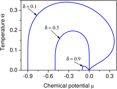
Figure 1: Lines of the NO phase instability (spinodals) with respect to the appearance of BE condensate in the $(\Theta,\mu)$ plane in the HCB limit at various excitation energies ($t_{0}=0$, $\lvert t_{0}^{\prime}\rvert=1$, $t_{0}^{\prime\prime}=0$).

We take into account (according to estimations made in [15, 25]) that boson wave functions in adjacent potential wells overlap in greater extent in the excited states compared to the ground ones. Accordingly, we shall put here $t_{0}=0$. For a centrosymmetric lattice and in the case of different parity of wave functions of ground and excited states we have also $t_{0}^{\prime\prime}=0$. Finally, we follow a usual convention of the BH model for optical lattices taking $t_{0}^{\prime}<0$. In this way equation (3.3) can be reduced to

$$\frac{\lvert t_{0}^{\prime}\rvert}{\delta-\mu}\frac{1-\mathrm{e}^{\beta(\mu-\delta)}}{1+\mathrm{e}^{\beta\mu}+\mathrm{e}^{\beta(\mu-\delta)}}=1.$$ (3.5)

Its solutions determine the stability region boundaries of the normal (NO) phase. Respective lines of spinodals are numerically calculated and presented in figure 1 (here and below the energy quantities are given in units of $\lvert t_{0}^{\prime}\rvert$).

As illustrated in figure 1, at $\delta<\lvert t_{0}^{\prime}\rvert$ spinodals surround an asymmetric area in the $(\Theta,\mu)$ plane which is located between the points $\mu=\delta-\lvert t_{0}^{\prime}\rvert$ and $\mu=0$ of the abscissa axis. In this region, the NO phase is unstable; this is connected with the appearance of BE condensate. At $\delta<\lvert t_{0}^{\prime}\rvert/2$ and $\mu>0$ the backward path of spinodal is observed and a lower temperature of the NO phase instability appears, thus suggesting a possibility of the SF phase existence in the intermediate temperature range (so-called ‘‘re-entrant transition’’). However, as will be shown further, in the mentioned region a real thermodynamic behaviour is even more complicated. The order of the NO-SF transition can change to the first one and the SF-phase remains stable up to the zero temperature.

4 Phase diagrams in MFA

For a more detailed treatment of the NO-SF transition issue, let us study the thermodynamics of the considered system in the HCB limit, thus reducing the problem to a three-state model with the Hamiltonian

$$\hat{H}=\sum_{ip}\lambda_{p}X_{i}^{pp}+\sum_{ij}t_{ij}X_{i}^{10}X_{j}^{01}+\sum_{ij}t_{ij}^{\prime}X_{i}^{20}X_{j}^{02}+\sum_{ij}t_{ij}^{\prime\prime}(X_{i}^{10}X_{j}^{02}+X_{i}^{20}X_{j}^{01}),$$ (4.1)

where the shorthand notations are used

$$|0\rangle\equiv|00\rangle,\;|1\rangle\equiv|10\rangle,\;|2\rangle\equiv|01\rangle;\qquad\lambda_{0}=\lambda_{00},\;\lambda_{1}=\lambda_{10},\;\lambda_{2}=\lambda_{01}\,.$$ (4.2)

Possibility of BE condensation will be studied in the MFA. Average values of creation (annihilation) operators for Bose particles in the ground or excited local state

$$\eta=\langle X_{i}^{10}\rangle=\langle X_{i}^{01}\rangle\;(\equiv\langle b_{i}\rangle),\qquad\xi=\langle X_{i}^{20}\rangle=\langle X_{i}^{02}\rangle\;(\equiv\langle c_{i}\rangle)$$ (4.3)

play the role of order parameters for the SF-phase. Hence, the mean-field Hamiltonian is as follows:

$$\hat{H}_{\mathrm{MF}} =-N(t_{0}\eta^{2}+t_{0}^{\prime}\xi^{2}+2t_{0}^{\prime\prime}\eta\xi)+\sum_{ip}\lambda_{p}X_{i}^{pp}$$

$$\quad+\sum_{i}\left[t_{0}\eta(X_{i}^{10}+X_{i}^{01})+t_{0}^{\prime}\xi(X_{i}^{20}+X_{i}^{02})+t_{0}^{\prime\prime}\xi(X_{i}^{10}+X_{i}^{01})+t_{0}^{\prime\prime}\eta(X_{i}^{20}+X_{i}^{02})\right].$$ (4.4)

Self-consistency equations for parameters $\eta$ and $\xi$

$$\eta=Z^{-1}\operatorname{Sp}[X_{i}^{10}\exp(-\beta\hat{H}_{\mathrm{MF}})],\qquad\xi=Z^{-1}\operatorname{Sp}[X_{i}^{20}\exp(-\beta\hat{H}_{\mathrm{MF}})]$$ (4.5)

are equivalent to the condition of minimum of the grand canonical potential $\Omega=-\Theta\ln Z$, where $Z=\operatorname{Sp}\exp(-\beta\hat{H}_{\mathrm{MF}})$.

Limiting our consideration to the case of particle hopping only through excited states ($t_{0}^{\prime}\neq 0$, $t_{0}=t_{0}^{\prime\prime}=0$) we can diagonalize Hamiltonian (4.4) by a rotation transformation

$$\left(\begin{array}[]{l}|0\rangle\\ |1\rangle\\ |2\rangle\end{array}\right)=\left(\begin{array}[]{ccc}\cos\vartheta&0&-\sin\vartheta\\ 0&1&0\\ \sin\vartheta&0&\cos\vartheta\end{array}\right)\left(\begin{array}[]{l}|\tilde{0}\rangle\\ |\tilde{1}\rangle\\ |\tilde{2}\rangle\end{array}\right),$$ (4.6)

where

$$\cos 2\vartheta=\frac{\lambda_{2}-\lambda_{0}}{\sqrt{(\lambda_{2}-\lambda_{0})^{2}+4(t_{0}^{\prime}\xi)^{2}}},\qquad\sin 2\vartheta=\frac{2\lvert t_{0}^{\prime}\rvert\xi}{\sqrt{(\lambda_{2}-\lambda_{0})^{2}+4(t_{0}^{\prime}\xi)^{2}}}$$ (4.7)

and $\lambda_{2}-\lambda_{0}=\delta-\mu$. In terms of operators $\widetilde{X}^{rs}=|\tilde{r}\rangle\langle\tilde{s}|$

$$\hat{H}_{\mathrm{MF}}=N\lvert t_{0}^{\prime}\rvert\xi^{2}+\sum_{ip}\tilde{\lambda}_{p}\widetilde{X}_{i}^{pp}.$$ (4.8)

New energies of single-site states are

$$\tilde{\lambda}_{0,2}=\frac{\delta-\mu}{2}\mp\sqrt{\left(\frac{\delta-\mu}{2}\right)^{2}+(t_{0}^{\prime}\xi)^{2}},\qquad\tilde{\lambda}_{1}=-\mu.$$ (4.9)

In the new basis

$$X_{i}^{02}+X_{i}^{20}=-(\widetilde{X}_{i}^{22}-\widetilde{X}_{i}^{00})\sin 2\vartheta+(\widetilde{X}_{i}^{20}-\widetilde{X}_{i}^{02})\cos 2\vartheta,$$ (4.10)

which yields after averaging

$$\xi=\frac{1}{2}\langle\widetilde{X}_{i}^{00}-\widetilde{X}_{i}^{22}\rangle\sin 2\vartheta.$$ (4.11)

Taking into account that $\langle\widetilde{X}^{pp}\rangle=Z^{-1}\exp(-\beta\tilde{\lambda}_{p})$, $Z=\sum_{p}\exp(-\beta\tilde{\lambda}_{p})$ we come to the equation for

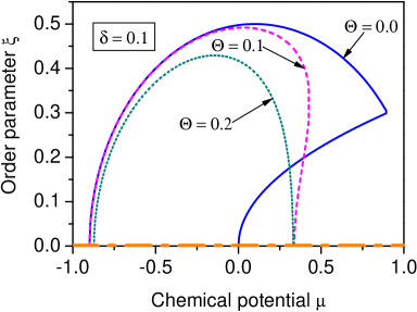
Figure 2: Dependences of the order parameter $\xi$ on the chemical potential $\mu$ for the reduced three-level (HCB) model at various temperatures indicating the possibility of the first order phase transition at low enough temperatures ($\delta=0.1$, $\lvert t_{0}^{\prime}\rvert=1$).

the order parameter $\xi$:

$$\xi=\frac{1}{Z}\,\frac{\lvert t_{0}^{\prime}\rvert\xi}{\sqrt{(\delta-\mu)^{2}+4(t_{0}^{\prime}\xi)^{2}}}\left(\mathrm{e}^{-\beta\tilde{\lambda}_{0}}-\mathrm{e}^{-\beta\tilde{\lambda}_{2}}\right).$$ (4.12)

Solution $\xi=0$ corresponds to the NO phase. A nonzero solution describing the BE condensate is obtained from the equation

$$\frac{1}{Z}\,\frac{\lvert t_{0}^{\prime}\rvert}{\sqrt{(\delta-\mu)^{2}+4(t_{0}^{\prime}\xi)^{2}}}\left(\mathrm{e}^{-\beta\tilde{\lambda}_{0}}-\mathrm{e}^{-\beta\tilde{\lambda}_{2}}\right)=1.$$ (4.13)

In the limit $\xi\to 0$ this equation determines the line where the order parameter for the SF phase tends to zero. One can readily see that it coincides with spinodal equation (3.5) thus defining the line of the second order NO-SF phase transition (when just the transition of such an order takes place).

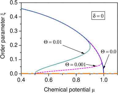
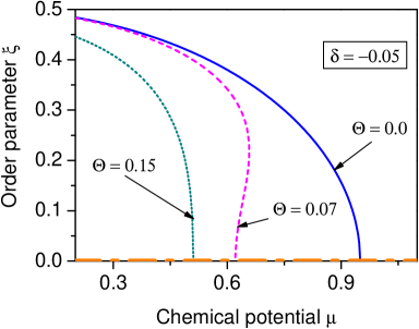
Figure 3: Low-temperature behaviour of the order parameter $\xi$ for the reduced three-level (HCB) model at zero and negative excitation energies $\delta$ and various temperatures ($\lvert t_{0}^{\prime}\rvert=1$).

Numerical solutions of equation (4.13) make it possible to study the behavior of the order parameter $\xi$ depending on chemical potential $\mu$ at various temperatures as illustrated in figure 2. In the main, at negative values of chemical potential the parameter $\xi$ changes smoothly and the phase transition to the SF phase is of the second order. But at $\mu\gtrsim 0$ and low enough temperatures, the $\xi(\mu)$ dependence has an S-like bend. In this case, the first order phase transition with an abrupt change of the parameter $\xi$ takes place. This phase transition occurs at a certain value of the chemical potential which could be calculated using the Maxwell rule or considering the minimum of the grand canonical potential $\Omega(\mu)$ as a function of the chemical potential (see below). Obviously, the point of $\xi$ nullification does not anymore correspond here to the phase transition.

Similar behaviour of the parameter $\xi$ holds even at zero excitation energy ($\delta=0$) where the first order phase transition remains for nonzero temperatures whereas at $T=0$ its order changes to the second one (figure 3). At negative values of $\delta$ (which corresponds to inversion of $\varepsilon$ and $\varepsilon^{\prime}$ levels and to hopping between ground states) the second order of the transition is preserved in the low-temperature region close to $T=0$ transforming to the first order transition at the temperature increase and recovering henceforth (figure 3).

Figure 4: Lines of the NO-SF phase transition in the $(\Theta,\mu)$ plane at various excitation energies $\delta$ ($\lvert t_{0}^{\prime}\rvert=1$).

Figure 5: An illustration of discrepancy between the spinodal curve and the real line of the first order phase transition for $\delta=0.01$ ($\lvert t_{0}^{\prime}\rvert=1$).

Figure 6: Appearance of two tricritical points at zero and negative values of excitation energy $\delta$ ($\lvert t_{0}^{\prime}\rvert=1$).

Figure 7: Lines of the NO-SF phase transition in the $(\lvert t_{0}^{\prime}\rvert,\mu)$ plane at various temperatures $\Theta$ (energy quantities are given in units of $\delta$).

Changes in the NO-SF phase transition order and localization of the corresponding tricritical points are depicted in figure 5, where phase diagrams are given for various values of the excitation energy $\delta$. At temperatures lower than tricritical, spinodal lines and phase transition curves come apart as one can see comparing figures 1 and 5. At small values of $\delta$, the discrepancy is quite significant (figure 5). In the case of $\delta<0$, two critical points appear at a certain distance; the latter tends to zero at $\delta=\delta_{\mathrm{crit}}\approx-0.12\lvert t_{0}^{\prime}\rvert$ and the first order phase transitions at a further increase of $\delta$ (figure 7) is suppressed.

Phase diagrams in the $(\lvert t_{0}^{\prime}\rvert,\mu)$ plane at various temperatures for $\delta>0$ are depicted in figure 7 with indication of tricritical points. In distinction to the standard two-level HCB model [34] (where the SF phase transition is of the second order) the diagrams are asymmetric. In the limit $T\to 0$ for $\mu>0$ the first order transition occurs at $\mu=(\sqrt{\delta}-\sqrt{\lvert t_{0}^{\prime}\rvert})^{2}$ (see the next section) whereas for $\mu<0$ they are of the second order on the line $\mu=\delta-\lvert t_{0}^{\prime}\rvert$.

5 Phase separation at fixed boson concentration

Let us consider now the thermodynamics of the model at a fixed concentration of Bose particles. We will utilize a connection between the concentration and the chemical potential of bosons which can be established using its definition in such a form

$$n \equiv\langle n_{i}^{b}+n_{i}^{c}\rangle=\langle X_{i}^{11}+X_{i}^{22}\rangle$$ (5.1)

or basing on the relationship

$$n =-\frac{\partial(\Omega/N)}{\partial\mu}\,.$$ (5.2)

In the first case similarly to equality (4.10) one can obtain a relation

$$X_{i}^{11}+X_{i}^{22}=\widetilde{X}_{i}^{11}+\widetilde{X}_{i}^{00}\sin^{2}\vartheta+\widetilde{X}_{i}^{22}\cos^{2}\vartheta+(\widetilde{X}_{i}^{02}+\widetilde{X}_{i}^{20})\sin\vartheta\cos\vartheta$$ (5.3)

which results in

$$n =\langle\widetilde{X}_{i}^{11}\rangle+\langle\widetilde{X}_{i}^{00}\rangle\sin^{2}\vartheta+\langle\widetilde{X}_{i}^{22}\rangle\cos^{2}\vartheta=$$

$$=\frac{1}{Z}\left\{\mathrm{e}^{-\beta\tilde{\lambda}_{1}}+\left[\frac{1}{2}-\frac{\delta-\mu}{2\sqrt{(\delta-\mu)^{2}+4(t_{0}^{\prime}\xi)^{2}}}\right]\mathrm{e}^{-\beta\tilde{\lambda}_{0}}+\left[\frac{1}{2}+\frac{\delta-\mu}{2\sqrt{(\delta-\mu)^{2}+4(t_{0}^{\prime}\xi)^{2}}}\right]\mathrm{e}^{-\beta\tilde{\lambda}_{2}}\right\}.$$ (5.4)

In the second case, taking into account that

$$\Omega/N=\lvert t_{0}^{\prime}\rvert\xi^{2}-\Theta\ln Z,\qquad Z=\mathrm{e}^{\beta\mu}+\mathrm{e}^{-\beta(\delta-\mu)/2}\cosh\beta\sqrt{\bigl{(}\textstyle\frac{\delta-\mu}{2}\bigr{)}^{2}+(t_{0}^{\prime}\xi)^{2}}$$ (5.5)

and differentiating with respect to $\mu$, one can come to the same expression as (5.4).

There are different relationships between $n$ and $\mu$ in NO and SF phases; in the last case, a nonzero value of $\xi$ (a solution of equation (4.13)) should be substituted into expression (5.4). Order parameter $\xi$ has a jump at the first order phase transition, so a stepwise change of concentration $n$ takes place. In the $n=\mathrm{const}$ regime (at the value of $n$ in the region of step) it means a phase separation into two phases with different concentrations: the NO phase ($\xi=0$ and a larger concentration of bosons) and the SF phase ($\xi\neq 0$ and their smaller concentration).

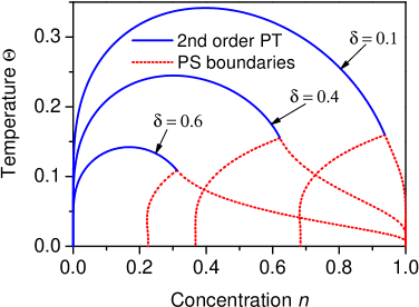
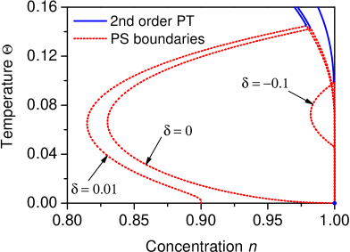
Figure 8: Lines of the NO-SF phase transition and the phase separation region in the $(\Theta,n)$ plane at various excitation energies $\delta$ including the case of small, zero and negative values of $\delta$ ($\lvert t_{0}^{\prime}\rvert=1$).

The above described situation is illustrated in figure 8, where the numerically calculated $(\Theta,n)$ phase diagrams are presented. At $\delta>0$, phase separation region spans up to tricritical temperatures. When $\delta$ goes to zero and finally reverses its sign, the shape of the separation region changes in a peculiar way moving off abscissa axis (figure 8). Now the phase separation begins at nonzero temperatures and vanishes at $\delta<\delta_{\mathrm{crit}}$; the line of the second order phase transition remains only. At the further increase of $\lvert\delta\rvert$ (in the $\mu<0$ region) the $(\Theta,n)$ diagram becomes more and more symmetric, approaching by its shape the diagram known for the usual HCB model [35] (see also [36]).

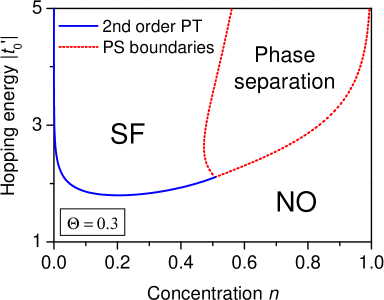
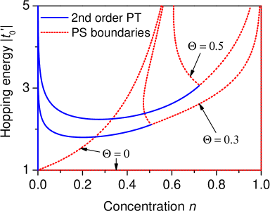
Figure 9: Phase diagram with the indication of possible phases (above) and lines of the NO-SF phase transition in the $(\lvert t_{0}^{\prime}\rvert,\mu)$ plane at various temperatures $\Theta$ (energy quantities are given in units of $\delta$).

Phase diagrams in the $(\lvert t_{0}^{\prime}\rvert,n)$ coordinates are given in figure 9 where the regions of NO, SF and separated phases are shown at various temperatures.

The case of the zero temperature can be studied more in detail in a pure analytic way. In this limit there are three branches of order parameter $\xi$ as a function of the chemical potential (see figure 2):

$$(1) \colon\xi=\frac{1}{2\lvert t_{0}^{\prime}\rvert}\sqrt{\lvert t_{0}^{\prime}\rvert^{2}-(\mu-\delta)^{2}},$$

$$(2) \colon\xi=\sqrt{\mu\delta}/\lvert t_{0}^{\prime}\rvert,$$

$$(3) \colon\xi=0.$$ (5.6)

After elimination of $\xi$ parameter, one can obtain the grand canonical potential $\Omega$ as follows:

$$(1) \colon\Omega/N=\frac{(\mu-\delta+\lvert t_{0}^{\prime}\rvert)^{2}}{4\lvert t_{0}^{\prime}\rvert},$$

$$(2) \colon\Omega/N=(\delta/\lvert t_{0}^{\prime}\rvert-1)\mu,$$

$$(3) \colon\Omega/N=\begin{cases}0,&\mu<0,\\ -\mu,&\mu>0.\end{cases}$$ (5.7)

Differentiating expressions (5.7) with respect to $\mu$ we have

$$(1) \colon n=\frac{1}{2}+\frac{\mu-\delta}{2\lvert t_{0}^{\prime}\rvert},$$

$$(2) \colon n=1-\delta/\lvert t_{0}^{\prime}\rvert,$$

$$(3) \colon n=\begin{cases}0,&\mu<0,\\ 1,&\mu>0.\end{cases}$$ (5.8)

At the first order phase transition from the SF phase to the NO phase, the order parameter $\xi$ jumps from branch (1) to branch (3). This occurs at the $\mu=\mu^{*}\equiv(\sqrt{\lvert t_{0}^{\prime}\rvert}-\sqrt{\delta})^{2}$ value given by equality of respective grand canonical potentials $\Omega_{(1)}=\Omega_{(3)}$. Then boson system separates into SF and NO phases with concentrations of bosons:

$$n_{\mathrm{SF}} =\frac{1}{2}+\frac{\mu^{*}-\delta}{2\lvert t_{0}^{\prime}\rvert},$$

$$n_{\mathrm{NO}} =1.$$ (5.9)

6 Discussion and conclusions

As was shown in this work, the transition to the SF phase (the phase with BE condensate) in the Bose-Hubbard model with two local states (the ground and excited ones) on the lattice site can be of the first order in the case, when the particle hopping takes place only in the excited band. Calculations and estimates for optical lattices give evidence of significant distinction between hopping parameters $t_{0}$ and $t_{1}$ in the ground and excited bands, respectively. It follows from estimates [25] that $t_{1}/t_{0}\approx 30-50$ depending on depth $V_{0}$ of local potential wells (one can produce effect on $V_{0}$ changing the intensity of laser beams which create an optical lattice). Similar results are obtained in the studies of quantum delocalization of the adsorbed hydrogen atoms. One can see from calculations [22, 23] of energy spectrum of the H-atom subsystem on the nickel surface that the ground-state band has a negligible bandwidth. At the same time, for excited bands, the bandwidth varies in the range from 15 to 45 meV (depending on the excited state symmetry and on the crystallographic orientation of metal surface), being mostly of the order of half the corresponding excitation energy $\Delta\varepsilon_{\alpha}=\varepsilon_{\alpha}-\varepsilon_{0}$ . There are, however, the cases of strong delocalization (e.g. H on the Ni(110) surface) where the excited bands overlap, and the width of the lowest one is of the same order as $\Delta\varepsilon_{\alpha}$ [22].

The values of hopping parameters greatly increase at the decrease of $V_{0}$; the distance between the local energy levels becomes smaller in this case (see [37, 38]). It is one of the possible ways of changing the relation between the hopping parameters and excitation energy ($\lvert t_{0}^{\prime}\rvert$ and $\delta$ in our model). Another possibility (discussed in [39]) is connected with an essential reduction of the energy gap between local $s$- and $p$-levels due to sufficiently strong interspecies Feshbach resonance in the presence of Fermi atoms added to the Bose system in optical lattice.

Along with investigation of BE condensation in the excited band (or bands $p_{x},p_{y}$ ($p_{x},p_{y},p_{z}$) in two- (three-) dimensional case) on condition that certain concentration of Bose-atoms has been created in the band by optical pumping [25, 38], an attempt was made in [40] to study the effect of excited bands on the physics of BE condensation in the lowest ($s$-) band (when the $s$-band hopping is taken into account). The case of finite values of the one-site interaction $U$ was considered. The possibility of the re-entrant behaviour of the MI-SF transition was claimed. However, the order of phase transition was not investigated; the consideration was restricted to the case of zero temperature. As we show in this work, re-entrant type dependence on $T$ or $\mu$ takes place only for spinodals and the return to the initial MI phase from the SF phase could be possible only in the case of the second order phase transitions. In reality, the order of phase transition changes to the first order in this region. In the HCB limit (no more than one particle per lattice site), it takes place mainly at positive values of chemical potential of particles; at $\mu<0$, the transition remains, for the most part, of the second order. The region of existence of SF phase is restricted, as a whole, to the interval $-\lvert t_{0}^{\prime}\rvert<\mu<\lvert t_{0}^{\prime}\rvert$, while excitation energy should obey the inequality $\delta<\lvert t_{0}^{\prime}\rvert$. We have constructed the corresponding phase diagrams and established localization of tricritical points, where the order of phase transition changes. The separation on SF and NO phases at the fixed particle concentration is investigated; the conditions of the appearance of phase-separated state are analyzed.

It should be mentioned that phase diagrams in figures 2–9 are close by their shape to the diagrams obtained in the framework of Bose-Hubbard model for Bose atoms with spin $S=1$ in optical lattices [29]. The excited levels are formed in that case by the higher spin single-site states and corresponding interactions of the ‘‘ferromagnetic’’ or ‘‘antiferromagnetic’’ type (the Hund-rule-like splitting), while the hopping parameter is taken the same for all bands. The similarity of the mentioned diagrams points out to the fact that the role of the excited states in the change of the phase transition order in going to the phase with the BE condensate is the same in both cases. Distinction, however, consists in another genesis of the single-site spectrum. In our model, in the limiting case of HCB there are no effects connected with the level splitting due to interaction; the excited single-particle states are taken by us into account instead.

The consideration developed in this work can be extended to the systems with the close or degenerate excited local levels. Generalization of the model by adding inter-site interactions is also important. It could even make it possible to take into consideration other phases (density-modulated or supersolid) besides NO and SF ones.

We finally emphasize that the hopping parameter $t_{ij}^{\prime}$ in the excited band can be positive; in particular, this concerns the $p$-bands [39]. In such a situation, the condensation takes place into states with wave vector $\vec{Q}$ on the boundary of the Brillouin zone, while the order parameters $\langle c_{Q}\rangle$, $\langle c_{Q}^{+}\rangle$ describe the modulated condensate. Since $t_{Q}^{\prime}=-t_{0}^{\prime}$ , the results obtained in this work are also valid (with $\lvert t_{Q}^{\prime}\rvert$ in place of $\lvert t_{0}^{\prime}\rvert$) in that case.