Deuteration as an evolutionary tracer in massive-star formation

Abstract

Context. Theory predicts, and observations confirm, that the column density ratio of a molecule containing D to its counterpart containing H can be used as an evolutionary tracer in the low-mass star formation process.

Aims. Since it remains unclear if the high-mass star formation process is a scaled-up version of the low-mass one, we investigated whether the relation between deuteration and evolution can be applied to the high-mass regime.

Methods. With the IRAM-30m telescope, we observed rotational transitions of N₂D⁺ and N₂H⁺ and derived the deuterated fraction in 27 cores within massive star-forming regions understood to represent different evolutionary stages of the massive-star formation process.

Results. Our results clearly indicate that the abundance of N₂D⁺ is higher at the pre–stellar/cluster stage, then drops during the formation of the protostellar object(s) as in the low-mass regime, remaining relatively constant during the ultra-compact HII region phase. The objects with the highest fractional abundance of N₂D⁺ are starless cores with properties very similar to typical pre–stellar cores of lower mass. The abundance of N₂D⁺ is lower in objects with higher gas temperatures as in the low-mass case but does not seem to depend on gas turbulence.

Conclusions. Our results indicate that the N₂D⁺-to-N₂H⁺ column density ratio can be used as an evolutionary indicator both in low- and high-mass star formation, and that the physical conditions that influence the abundance of deuterated species likely evolve similarly along the processes that lead to the formation of both low- and high-mass stars.

1 Introduction

The study of deuterated molecules is an extremely useful probe of the physical conditions in star-forming regions. Deuterated species are readily produced in molecular environments characterised by low temperatures ($T\leq 20$ K) and CO depletion (Millar et al. 1989). These physical/chemical properties are commonly observed in low-mass pre–stellar cores (starless cores on the verge of forming stars), where the deuterated fraction (hereafter $D_{\rm frac}$) of non-depleted molecules, defined as the column density ratio of one species containing deuterium to its counterpart containing hydrogen, is orders of magnitude larger than the [D/H] interstellar abundance (of the order of $\sim 10^{-5}$, Oliveira et al. 2003). Caselli (2002a) found a theoretical relation between $D_{\rm frac}$ and the core evolution in the low-mass case. This relation predicts that $D_{\rm frac}$ increases when the starless core evolves towards the onset of gravitational collapse because, as the core density profile becomes more and more centrally peaked, freeze-out of CO increases in the core centre and hence the abundance of deuterated molecules is greatly enhanced. When the young stellar object formed at the core centre begins to heat its surroundings, the CO evaporated from dust grains starts to destroy the deuterated species and $D_{\rm frac}$ decreases. Observations of both starless cores and cores with already formed protostars confirm the theoretical predictions in the low-mass regime: the pre–stellar cores closest to gravitational collapse have the highest $D_{\rm frac}$ (Crapsi et al. 2005), while $D_{\rm frac}$ is lower in cores associated with Class 0/I protostars, and the coldest (i.e. the youngest) objects possess the largest $D_{\rm frac}$, again in agreement with the predictions of chemical models (Emprechtinger et al. 2009, Friesen et al. 2010). On the basis of these results, $D_{\rm frac}$ can be considered as an evolutionary tracer of the low-mass star formation process before and after the formation of the protostellar object.

Can this result be applied to the high-mass regime? This question is difficult to answer because the massive-star formation process is still not well-understood: large distances ($\geq 1$ kpc), high extinction and clustered environments make observations of the process challenging (Beuther et al 2007a, Zinnecker & Yorke 2007). Observationally, the study of Pillai et al. (2007), performed with the Effelsberg and IRAM-30m telescopes, measured high values of $D_{\rm frac}$ ($\sim 0.2$) from deuterated ammonia in infrared dark clouds, which are understood to represent the earliest stages of massive star and stellar cluster formation. In more evolved objects, from IRAM-30m observations, Fontani et al. (2006) measured smaller values of $D_{\rm frac}$ ($\sim 10^{-2}$) from the ratio N₂D⁺/N₂H⁺, which are nevertheless much larger than the D/H interstellar abundance. Despite these efforts, no systematic study of the [D/H] ratio across all stages of high-mass star formation has yet been carried out.

In this letter, we present the first study of the relation between deuterated fraction and evolution in a statistically significant sample of cores embedded in high-mass star forming regions spanning a wide range of evolutionary stages, from high-mass starless core candidates (HMSCs) to high-mass protostellar objects (HMPOs) and ultracompact (UC) HII regions (for a definition of these stages see e.g. Beuther et al 2007a). This goal was achieved by observing rotational transitions of N₂H⁺ and N₂D⁺ with the IRAM-30m telescope. We chose these species because N₂D⁺ can be formed from N₂H⁺ only in the gas phase, tracing cold and dense regions more precisely than deuterated NH₃, which can also be formed on dust grains (e.g. Aikawa et al. 2005) and then evaporates by heating from nearby active star-formation. Even though the observations are obtained with low angular resolution, the objects observed in the survey were carefully selected to limit as much as possible any emission arising from adjacent objects.

2 Source selection and observations

The source list is in Table A-1, where we give the source coordinates, the distance, the bolometric luminosity, and the reference papers. We observed 27 molecular cores divided into: ten HMSCs, ten HMPOs, and seven UC HII regions. The source coordinates were centred towards either (interferometric) infrared/millimeter/centimeter continuum peaks or high-density gas tracer peaks (NH₃ with VLA, N₂H⁺ with CARMA or PdBI) identified in images with angular resolutions comparable to or better than 6″, either from the literature or from observations not yet published. In general, we rejected objects whose emission peaks were separated by less than $\sim 8$^′′ from another peak of a dense molecular gas tracer. This selection criterion was adopted to avoid or limit as much as possible the presence of multiple cores within the IRAM-30m beam(s). The evolutionary stage of each source was established based on a collection of evidence: HMSCs are massive cores embedded in infrared dark-clouds or other massive star forming regions not associated with indicators of ongoing star formation (embedded infrared sources, outflows, masers); HMPOs are associated with interferometric powerful outflows, and/or infrared sources, and/or faint ($S_{\nu}$ at 3.6 cm $<1$mJy) radio continuum emission likely tracing a radio-jet; and UC HIIs must be associated with a stronger radio-continuum ($S_{\nu}$ at 3.6 cm $\geq$ 1 mJy) that probably traces gas photoionised by a young massive star. We did not include evolved HII regions that have already dissipated the associated molecular core. We also limited the sample to sources at distances of less than $\sim 5$ kpc. We stress that the three categories must be regarded with caution because it can be difficult to determine the relative evolutionary stage. This caveat applies especially to HMPOs and UC HII regions, whose evolutionary distinction is not always a clear cut (see e.g. Beuther et al. 2007a). Among the HMSCs, three sources (AFGL5142- EC, 05358-mm3, and I22134-G) have been defined as ”warm” in Table A-1: we explain the peculiarity of these sources in Sect. 3. The observations of the 27 cores listed in Table A-1 were carried out with the IRAM-30m telescope in two main observing runs (February 2 to 4, June 19 to 21, 2010), and several additional hours allocated during three Herapool weeks (December 2009, January 2010, and November 2010). We observed the N₂H⁺ (3–2), N₂H⁺ (1–0), and N₂D⁺ (2–1) transitions. The main observational parameters of these lines are given in Table A-2. The observations were made in wobbler–switching mode. Pointing was checked every hour. The data were calibrated with the chopper wheel technique (see Kutner & Ulich 1981), with a calibration uncertainty of $\sim 20-30\%$. The spectra were obtained in antenna temperature units, $T_{\rm A}^{*}$, and then converted to main beam brightness temperature, $T_{\rm MB}$, via the relation $T_{\rm A}^{*}=T_{\rm MB}\,\eta_{\rm MB}$, where $\eta_{\rm MB}=B_{\rm eff}/F_{\rm eff}$ is 0.74 for N₂D⁺ (2–1), 0.53 for N₂H⁺ (3–2) and 0.88 for N₂H⁺ (1–0) lines, respectively. All observed transitions possess hyperfine structure. To take this into account, we fitted the lines using METHOD HFS of the CLASS program, which is part of the GILDAS software developed at the IRAM and the Observatoire de Grenoble. This method assumes that all the hyperfine components have the same excitation temperature and width, and that their separation is fixed to the laboratory value. The method also provides an estimate of the optical depth of the line, based on the intensity ratio of the different hyperfine components. For the faintest N₂D⁺ lines, for which the hfs method gives poor results, the lines were fitted assuming a Gaussian shape.

3 Results and discussion: is deuteration an evolutionary indicator of massive star formation?

The spectra of N₂D⁺ (2–1) and N₂H⁺ (3–2) for all sources detected in N₂D⁺ are shown in Figures B-1 – B-6. We detected N₂H⁺ (3–2) emission in all sources. We also found a remarkably high detection rate in the N₂D⁺ (2–1) line: 100$\%$ in HMSCs, 64$\%$ in HMPOs, and 100$\%$ in UC HII regions. Such a high detection rate indicates that deuterated gas is present at every stage of the massive star and star cluster formation process, even in the surroundings of UC HII regions where the gas is expected to be hotter and more chemically evolved. Even though for 12 sources we also observed the N₂H⁺ (1–0) transition, we always computed the column density of N₂H⁺ and the deuterated fraction from the (3–2) line given its smaller telescope beam, to limit the contribution of nearby sources as much as possible. An overall presentation of the data obtained, and a deeper analysis of all physical parameters, will be given in a forthcoming paper. We derived the N₂H⁺ and N₂D⁺ column densities, $N({\rm N_{2}H^{+}})$ and $N({\rm N_{2}D^{+}})$, from the line integrated intensity following the method described in the appendix of Caselli et al. (2002b). Thanks to the selection criteria for our sources, for which interferometric maps of dense gas are available for most of the regions, a first estimate of the filling factor could be computed. However, because maps of the two transitions used to derive $D_{\rm frac}$  have not yet been performed (except for I22134-VLA1), the source size was determined from interferometric measurements of NH₃(2,2). This assumption seems reasonable because this line traces gas with physical conditions similar to those of N₂H⁺ (3–2) and N₂D⁺ (2–1). To take into account the possible effects of the evolutionary stage on the source size, we also computed an average diameter for each evolutionary group. This turns out to be: 6.5″ for HMSCs, 4.1″ for HMPOs, and 5.5″ for UC HIIs (Busquet 2010, Busquet et al. 2011, Sánchez-Monge 2011, Palau et al. 2007, 2010). We stress that these angular diameters are consistent with the (few) N₂H⁺ and N₂D⁺ interferometric observations published to date (e.g. see the case of IRAS 05345+3157, Fontani et al. 2008). The N₂H⁺ and N₂D⁺ column densities, their ratio ($D_{\rm frac}$), as well as the line parameters used in the derivation of the column densities, are listed in Table A-3.

The method assumes a constant excitation temperature, $T_{\rm ex}$. For the N₂H⁺ lines, $T_{\rm ex}$ was derived directly from the parameters given by the hyperfine fitting procedure corrected for the filling factor (see the CLASS user manual for details: http://iram.fr/IRAMFR/GILDAS/doc/html/class-html/class.html). The procedure, however, cannot provide good estimates for optically thin transitions or transitions with opacity ($\tau$) not well-constrained (e.g. with relative uncertainty larger than $30\%$). For these, we were obliged to assume a value for $T_{\rm ex}$ (for details, see the notes of Table A-3). For the N₂D⁺ (2–1) lines we were unable to derive $T_{\rm ex}$ from the fitting procedure for almost all sources because $\tau$ is either too small or too uncertain. In 3 cases only was the optical depth of the N₂D⁺ (2–1) transition well-determined, and so is $T_{\rm ex}$: in two of these objects we found a close agreement between the estimates derived from the N₂D⁺ (2–1) and the N₂H⁺ (3–2) transitions. Therefore, the N₂D⁺ column density of each source was computed assuming the same $T_{\rm ex}$ as for N₂H⁺. Since N₂D⁺ (2–1) and N₂H⁺ (3–2) have similar critical densities and we measure similar $T_{\rm ex}$ for both transitions, the two lines approximately trace similar material, so that computing $D_{\rm frac}$ using them is a reasonable approach. The N₂H⁺ column densities are on average of the order of $10^{13-14}$ cm^-2, and the N₂D⁺ column densities are of order $10^{12-13}$ cm^-2. Both values are consistent with similar observations towards massive star forming regions (e.g. Fontani et al. 2006). The measured $T_{\rm ex}$ corrected for filling factor are between $\sim 7$ and $\sim 50$ K and agree, on average, with the kinetic temperatures measured from ammonia, except for the colder HMSCs for which they are a factor of $\sim 2$ lower.

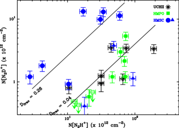
Figure 1: N₂D⁺ column density versus N₂H⁺ column density. Blue symbols correspond to HMSCs (triangles: ”warm” cores, see text); green squares show HMPOs (open squares are upper limits); black asterisks correspond to UC HII regions. The two lines indicate the average values of $D_{\rm frac}$ for the HMSC group (i.e. 0.26) and that of both the HMPO and UC HII groups (i.e. 0.04).

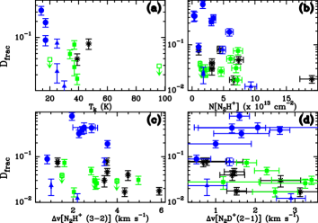
Figure 2: Deuterated fraction, $D_{\rm frac}$= $N$(N₂D⁺)$/N$(N₂H⁺), as a function of several parameters: kinetic temperature (a), N(N₂H⁺) (b), N₂H⁺ (3–2) line width (c) and N₂D⁺ (2–1) line width (d). The symbols have the same meaning as in Fig. 1. For some sources, the errorbars are not visible because they are smaller than the symbol size. In panel (a), only the sources with temperature derived from VLA ammonia observations are plotted.

The deuterated fraction for the three evolutionary groups is shown in Fig. 1, where we plot $N$(N₂D⁺) against $N$(N₂H⁺). There is a statistically significant separation between the HMSC group, which has the highest average $D_{\rm frac}$ (mean value $\sim 0.26$, $\sigma=0.22$), and the HMPOs and UC HII groups, which have similar average deuterated fraction: mean $D_{\rm frac}$$=0.037$ ($\sigma=0.017$) for HMPOs, and mean $D_{\rm frac}$= 0.044 ($\sigma=0.024$) for UC HII regions. Both are about an order of magnitude smaller than that associated with HMSCs. A closer inspection of the data using the Kolmogorov-Smirnov statistical test shows that the separation in $D_{\rm frac}$ between the HMSC group and that including both HMPOs and UC HII regions is indeed statistically significant: the test shows that the probability of the distributions being the same is very low ($P\sim 0.004$). This is strong evidence that the two groups differ statistically. Therefore, massive cores without stars have larger abundances of N₂D⁺ than cores with already formed massive (proto-)stars or proto-clusters. The abundance of N₂D⁺, however, seems to remain constant, within the uncertainties, after the formation of the protostellar object until the UC HII region phase. That $D_{\rm frac}$ is of the order of $\sim 0.2-0.3$, on average, in HMSCs, and then drops by an order of magnitude after the onset of star formation, indicates that the physical conditions acting on the abundance of deuterated species (i.e. density and temperature) evolve similarly along both the low- and high-mass star formation processes (see e.g. Crapsi et al. 2005 and Emprechtinger et al. 2009).

Another interesting aspect emerging from Fig. 1 is that the three HMSCs defined as ”warm” in Table A-1 (AFGL5142-EC, 05358-mm3, and I22134-G, marked as triangles in the figure) have $D_{\rm frac}$ almost an order of magnitude smaller than the others. These differ from the rest of the sub-sample of HMSCs because they have temperatures $T_{\rm k}$ $>20$ K (see Table A-3 and panel (a) in Fig. 2). High angular resolution studies indicate that they could be externally heated (Zhang et al. 2002, Busquet 2010, Sánchez-Monge 2011), so that they are likely to be perturbed by nearby star formation and we expect their properties to be different from those of the other, more quiescent cores. An anticorrelation between $D_{\rm frac}$ and the distance to heating sources such as embedded protostars was found in the cluster-forming Ophiuchus-B clump by Friesen et al (2010). Our study tends to confirm the Friesen et al.’s finding, even though the poor statistics does not allow us to drive firm conclusions. We also point out that the four cores selected from the Butler & Tan (2009) work (G034-G2, G034-F1, G034-F2, G028-C1) have the highest values of all measured $D_{\rm frac}$ and lie in infrared-dark regions, away from active star formation. These four cores are hence very similar to the prototype low-mass ’pre-stellar cores’ (e.g. L1544, L694–2, see Crapsi et al. 2005) and we propose that these are good ’massive pre–stellar core’ candidates.

In Fig. 2, we plot $D_{\rm frac}$ as a function of several parameters: the kinetic temperature, the N₂H⁺ column density, and the line widths derived from both N₂H⁺ and N₂D⁺. To search for possible (anti-)correlations between these parameters, we performed two statistical tests: the Kendall’s $\tau$ and the Spearman’s $\rho$ rank correlation tests . For $T_{\rm k}$, the tests were applied to all sources in our survey with gas temperature derived from VLA interferometric ammonia observations (see Table A-3). As it can be inferred from panel (a) of Fig. 2, $D_{\rm frac}$ and $T_{\rm k}$ are slightly anti-correlated ($\tau=-0.38$, $\rho$= $-0.50$), and $D_{\rm frac}$ is also anti-correlated with the N₂H⁺ column density ($\tau=-0.43$, $\rho$= $-0.60$, panel (b) in Fig. 2). We also find a very faint anticorrelation between $D_{\rm frac}$ and the N₂H⁺ line width ($\tau=-0.17$, $\rho=-0.23$) and between $D_{\rm frac}$ and the N₂D⁺ line width ($\tau=-0.25$, $\rho=-0.35$) (panels (c) and (d) in in Fig. 2, respectively). In particular, this latter is difficult to trust being affected by large uncertainties in the N₂D⁺ line widths. Emprechtinger et al. (2009) suggested that in low-mass star forming cores the deuteration is higher in colder and more quiescent cores, according to the predictions of theoretical models. A similar trend was found also in a small sample of seven massive star-forming clumps by Fontani et al. (2006) including both HMPOs and UC HII regions but not HMSCs. That the warmer sources have lower $D_{\rm frac}$ is not surprising and can be explained by the CO freeze-out and the chemical reactions leading to the enhancement of deuterium abundance being strongly depressed when the temperature increases (Caselli et al. 2008). The lack of correlation between deuterated fraction and line widths tells us that the deuterium fractionation process is independent of the gas turbulence. This result agrees with high-angular resolution observations of cluster-forming regions (Fontani et al.  2009, Busquet et al. 2010), but given the large uncertainties (especially on the N₂D⁺ line widths), the conclusions must be interpreted with caution. We speculate that the anticorrelation between $D_{\rm frac}$ and $N$(N₂H⁺) could indicate that, assuming that $D_{\rm frac}$ decreases in the protostellar phase, the N₂H⁺ column density increases during the younger and most embedded period of the protostellar phase, as suggested by Busquet (2010) for a different sample of sources.

In summary, our findings indicate that the physical conditions acting on the abundance of deuterated species (i.e. density and temperature) evolve similarly during both the low- and high-mass star formation process. To confirm this, several questions however need to be answered: in HMSCs, do the N₂D⁺ and N₂H⁺ emission peak at dust emission peak as in low-mass pre–stellar cores? What is the nature of the N₂D⁺ emission in evolved objects (HMPOs and UC HII regions)? Is the emission extended or fragmented into several condensations (as found in the few massive star forming regions observed with interferometers)? To answer these questions, higher angular resolution observations are necessary. On the theoretical side, we also need to investigate this proposed evolutionary sequence using astrochemical models.

Acknowledgments. We are grateful to the IRAM-30m telescope staff for their help during the observations. Many thanks to the anonymous Referee for his/her comments that significantly improved the work. FF has received funding from the European Community’s Seventh Framework Programme (FP7/2007–2013) under grant agreement No. 229517. AP, AS-M and GB are supported by the Spanish MICINN grant AYA2008-06189-C03 (co-funded with FEDER funds). AP is supported by JAEDoc CSIC fellowship co-funded with the European Social Fund. GB is funded by the Italian Space Agency (ASI) with contract ASI-I/005/07/1. MA acknowledges support from the Swiss National Science Foundation (grants PP002-110504 and PP00P2-130188)

Appendix A: Tables

Table A-1 contains the list of the observed sources selected as explained in Sect. 2 of the main body text, and give some information extracted from the literature about the star forming regions in which the sources lie. Table A-2 presents the observed transitions and some main technical observational parameters. Table A-3 shows the results of the fitting procedure to the N₂D⁺ (2–1) and N₂H⁺ (3–2) lines (see Sect. 2 of the main body text) of all sources, and the physical parameters derived from these results, namely the N₂H⁺ and N₂D⁺ column densities and their ratio, $D_{\rm frac}$. Other parameters discussed in Sect. 3 of the main body text are also listed.

Table A-1: list of the observed sources. Col. 4 shows the velocity at which we centred the spectra, corresponding to the systemic velocity. Cols. 5 and 6 give the source distance and bolometric luminosity (respectively) of the associated star forming region. This latter is a very rough first approximation of the core luminosity because it is based on infrared measurements having poor angular resolution. We adopt as source names those used in the reference papers listed in Col. 7.

source	RA(J2000)	Dec(J2000)	$V_{\rm LSR}$	$d$	$L_{\rm bol}$	Ref.
	h m s	$o$ $\prime$ $\prime\prime$	km s-1	kpc	$L_{\odot}$
HMSC
I00117-MM2	00:14:26.3	+64:28:28	$-36.3$	1.8	$10^{3.1}$	(1)
AFGL5142-EC	05:30:48.7	+33:47:53	$-3.9$	1.8	$10^{3.6}$	(2)
05358-mm3	05:39:12.5	+35:45:55	$-17.6$	1.8	$10^{3.8}$	(3,11)
G034-G2(MM2)	18:56:50.0	+01:23:08	$+43.6$	2.9	$10^{1.6}$	(4)
G034-F1(MM8)	18:53:19.1	+01:26:53	$+57.7$	3.7	$10^{1.9}$	(4)
G034-F2(MM7)	18:53:16.5	+01:26:10	$+57.7$	3.7	–	(4)
G028-C1(MM9)	18:42:46.9	$-$04:04:08	$+78.3$	5.0	–	(4)
I20293-WC	20:31:10.7	+40:03:28	$+6.3$	2.0	$10^{3.6}$	(5,6)
I22134-G	22:15:10.5	+58:48:59	$-18.3$	2.6	$10^{4.1}$	(7)
I22134-B	22:15:05.8	+58:48:59	$-18.3$	2.6	$10^{4.1}$	(7)
HMPO
I00117-MM1	00:14:26.1	+64:28:44	$-36.3$	1.8	$10^{3.1}$	(1)
I04579-VLA1	05:01:39.9	+47:07:21	$-17.0$	2.5	$10^{3.6}$	(8)
AFGL5142-MM	05:30:48.0	+33:47:54	$-3.9$	1.8	$10^{3.6}$	(2)
05358-mm1	05:39:13.1	+35:45:51	$-17.6$	1.8	$10^{3.8}$	(3)
18089–1732	18:11:51.4	$-$17:31:28	$+32.7$	3.6	$10^{4.5}$	(9)
18517+0437	18:54:14.2	+04:41:41	$+43.7$	2.9	$10^{4.1}$	(10)
G75-core	20:21:44.0	+37:26:38	$+0.2$	3.8	$10^{4.8}$	(11,12)
I20293-MM1	20:31:12.8	+40:03:23	$+6.3$	2.0	$10^{3.6}$	(5)
I21307	21:32:30.6	+51:02:16	$-46.7$	3.2	$10^{3.6}$	(13)
I23385	23:40:54.5	+61:10:28	$-50.5$	4.9	$10^{4.2}$	(14)
UC HII
G5.89–0.39	18:00:30.5	$-$24:04:01	$+9.0$	1.28	$10^{5.1}$	(15,16)
I19035-VLA1	19:06:01.5	+06:46:35	$+32.4$	2.2	$10^{3.9}$	(11)
19410+2336	19:43:11.4	+23:44:06	$+22.4$	2.1	$10^{4.0}$	(17)
ON1	20:10:09.1	+31:31:36	$+12.0$	2.5	$10^{4.3}$	(18,19)
I22134-VLA1	22:15:09.2	+58:49:08	$-18.3$	2.6	$10^{4.1}$	(11)
23033+5951	23:05:24.6	+60:08:09	$-53.0$	3.5	$10^{4.0}$	(17)
NGC7538-IRS9	23:14:01.8	+61:27:20	$-57.0$	2.8	$10^{4.6}$	(8)

Table A-2: Observed transitions and technical parameters

molecular	frequency	HPBW	$\Delta v$	Bandwidth
transition	(GHz)	(′′)	(km s-1)	(km s-1)
N2H+ (1$-$0)	93.17376	26	$0.126$	$230$
N2H+ (3$-$2)	279.51186	9	$0.042$	$77$
N2D+ (2$-$1)	154.21718	16	$0.076$	$139$

Table A-3: Observational and derived line parameters: Cols. 2–6 list integrated intensity over all the hyperfine components ($\int T_{\rm MB}{\rm d}v$), peak velocity ($V_{\rm LSR}$), full width at half maximum (FWHM) corrected for hyperfine splitting, opacity ($\tau$) and excitation temperature ($T_{\rm ex}$), from N₂H⁺ (3–2); Cols. 7, 8 and 9 list $\int T_{\rm MB}{\rm d}v$, $V_{\rm LSR}$ and FWHM for the N₂D⁺ (2–1) lines. In cols 10 and 11 we give the N₂H⁺ and N₂D⁺ column densities, respectively, and their ratio ($D_{\rm frac}$) is given in Col. 12. Col. 13 shows the kinetic temperature ($T_{\rm k}$) measured from ammonia observations. Uncertainties are given in parentheses.

		N2H+ (3–2)						N2D+ (2–1)
	source	$\int T_{\rm MB}{\rm d}v$	$V_{\rm LSR}$	FWHM	$\tau$	$T_{\rm ex}$		$\int T_{\rm MB}{\rm d}v$	$V_{\rm LSR}$	FWHM	N(N2H+)	N(N2D+)	$D_{\rm frac}$	$T_{\rm k}$
		(K km s-1)	(km s-1)	(km s-1)		(K)		(K km s-1)	(km s-1)	(km s-1)	($\times 10^{13}$ cm-2)	($\times 10^{12}$ cm-2)		(K)
HMSCs	I00117-MM2	2.9(0.1)	–50.51(0.01)	2.27(0.04)	$<$0.1	7		0.48(0.02)	–50(1)	1.65(0.7)	3.1(0.3)	10(1)	0.32(0.06)	14
	AFGL5142-EC	20.7(0.1)	–17.21(0.01)	3.42(0.01)	0.51(0.01)	44.1(0.1)		0.48(0.03)	–17.73(0.04)	1.35(0.1)	4.8(0.5)	3.8(0.6)	0.08(0.01)	25
	05358-mm3	43.0(0.1)	–30.34(0.01)	2.200(0.003)	5(2)	34(4)		0.16(0.02)	–30.5(0.2)	2.9(0.4)	9.3(0.9)	1.1(0.3)	0.012(0.003)	30
	G034-G2(MM2)	2.0(0.1)	27.2(0.02)	1.950(0.003)	1.51(0.01)	7.57(0.03)		0.76(0.03)	26.80(0.08)	1.6(0.3)	1.7(0.2)	13(2)	0.7(0.2)	$-$
	G034-F1(MM8)	1.65(0.05)	43.3(0.1)	2.84(0.3)	$<$0.1	16		0.25(0.03)	42.7(0.2)	1.4(0.9)	0.42(0.04)	1.8(0.3)	0.43(0.09)	$-$
	G034-F2(MM7)	1.08(0.08)	43.1(0.2)	2.5(0.5)	–	16		0.17(0.03)	42(4)	2.0(1.5)	0.28(0.03)	1.2(0.3)	0.4(0.1)	$-$
	G028-C1(MM9)	2.4(0.1)	65.32(0.03)	2.4(0.2)	3(1)	6.4(0.4)		0.50(0.03)	65.10(0.08)	2.6(0.3)	3.4(0.3)	13(2)	0.38(0.07)	17
	I20293-WC	9.4(0.1)	–7.510(0.008)	3.560(0.003)	$<$0.1	8.5		0.82(0.03)	–7.7(0.3)	1.0(0.9)	5.9(0.6)	11(2)	0.19(0.3)	17
	I22134-G	6.9(0.1)	–33.20(0.01)	1.01(0.02)	3.3(0.2)	15.9(0.3)		0.06(0.01)	–34.7(0.2)	0.8(0.5)	1.8(0.2)	0.4(0.2)	0.023(0.009)	25
	I22134-B	2.4(0.1)	–33.3(0.04)	0.83(0.03)	2.3(0.3)	10.4(0.4)		0.09(0.02)	–33.8(0.06)	0.5(0.4)	1.0(0.1)	0.9(0.2)	0.09(0.02)	17
HMPOs	I00117-MM1	5.5(0.1)	–50.89(0.01)	1.50(0.04)	2.4(0.3)	19.3(0.4)		$\leq 0.07$	–	$--$	1.26(0.1)	$\leq 0.5$	$\leq 0.04$	20
	I04579-VLA1	1.23(0.02)	–32.51(0.06)	1.8(0.2)	$<$0.1	74	–	$\leq 0.14$		$--$	0.4(0.05)	$\leq 1.5$	$\leq 0.4$	74
	AFGL5142-MM	27.2(0.1)	–17.470(0.004)	2.820(0.006)	3.4(0.1)	39.24(0.01)		0.40(0.02)	–17.7(0.1)	2.3(0.3)	6.1(0.6)	3.0(0.5)	0.049(0.009)	34
	05358-mm1	30.3(0.1)	–30.588(0.003)	2.040(0.003)	5(1)	46(2)		0.15(0.02)	–30.7(0.3)	2.5(0.6)	7.2(0.7)	1.2(0.2)	0.017(0.004)	39
	18089–1732	31.4(0.2)	17.40(0.004)	4.960(0.001)	$<$0.1	38		0.29(0.03)	18.3(0.6)	3(1)	7.0(0.7)	2.2(0.3)	0.031(0.006)	38
	18517+0437	19.2(0.1)	29.44(0.03)	3.08(0.01)	$<$0.1	47		0.15(0.02)	29.2(0.5)	3(1)	4.6(0.5)	1.2(0.2)	0.026(0.006)	$-$
	G75-core	6.5(0.1)	–14.99(0.02)	3.99(0.04)	$<$0.1	96		$\leq 0.05$	–	$--$	2.4(0.2)	$\leq 0.69$	$\leq 0.029$	96
	I20293-MM1	29.6(0.1)	–8.31(0.02)	1.610(0.002)	6.4(0.1)	50.1(0.1)		0.64(0.03)	–9.31(0.08)	1.8(0.3)	7.3(0.7)	5.4(0.8)	0.07(0.01)	37
	I21307	6.5(0.1)	–61.29(0.02)	2.98(0.05)	$<$0.1	21		$\leq 0.06$	–	$--$	1.5(0.1)	$\leq 0.4$	$\leq 0.03$	21
	I23385	9.41(0.08)	–64.88(0.01)	3.02(0.03)	$<$0.1	37		0.08(0.05)	–63(3)	1.2(0.9)	2.1(0.2)	0.6(0.1)	0.028(0.009)	37
UC HII	G5.89–0.39	84.1(0.3)	–5.820(0.003)	5.900(0.009)	$<$0.1	20		0.50(0.03)	–7.4(0.1)	1.5(0.3)	19(2)	3.4(0.5)	0.018(0.003)	$-$
	I19035-VLA1	13.7(0.2)	17.62(0.01)	4.49(0.03)	$<$0.1	19.0(0.2)		0.18(0.03)	17.5(0.1)	1.4(0.3)	3.2(0.3)	1.3(0.3)	0.04(0.01)	39
	19410+2336	33.3(0.1)	7.90(0.005)	3.550(0.001)	$<$0.1	21		0.52(0.05)	7.5(0.08)	1.5(0.3)	7.4(0.7)	3.5(0.5)	0.047(0.009)	21
	ON1	30.9(0.2)	–2.421(0.001)	4.340(0.001)	$<$0.1	26		0.17(0.05)	–3.3(0.9)	3.13(1.65)	6.6(0.7)	1.1(0.2)	0.017(0.004)	26
	I22134-VLA1	2.5(0.08)	–33.11(0.01)	1.30(0.06)	1.9(0.4)	10.6(0.5)		0.08(0.01)	–34.2(0.4)	0.7(1.0)	1.0(0.1)	0.8(0.2)	0.08(0.02)	47
	23033+5951	19.6(0.1)	–67.72(0.03)	3.530(0.002)	$<$0.1	25		0.52(0.02)	–68.2(0.5)	0.8(0.5)	4.4(0.4)	3.5(0.5)	0.08(0.02)	25
	NGC7538-IRS9	13.9(0.1)	–71.814(0.006)	3.42(0.03)	$<$0.1	20		0.14(0.02)	–72(2)	2.6(0.5)	3.2(0.3)	0.9(0.2)	0.030(0.008)	$-$

Appendix B: Spectra

In this appendix, all spectra of N₂D⁺ (2–1) and N₂H⁺ (3–2) transitions, for the sources detected in both transitions, are shown.

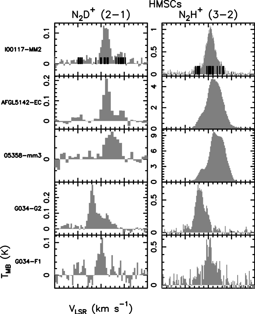
Figure B-1: Spectra of N₂D⁺ (2–1) and N₂H⁺ (3–2) obtained towards the sources classified as HMSCs. For each spectrum, the velocity interval shown is $\pm 10$ km s^-1 from the systemic velocity listed in Table A-1. The y-axis is in main beam brightness temperature units. In the spectra of I00117-MM2, the vertical bars show the position of the hyperfine components.

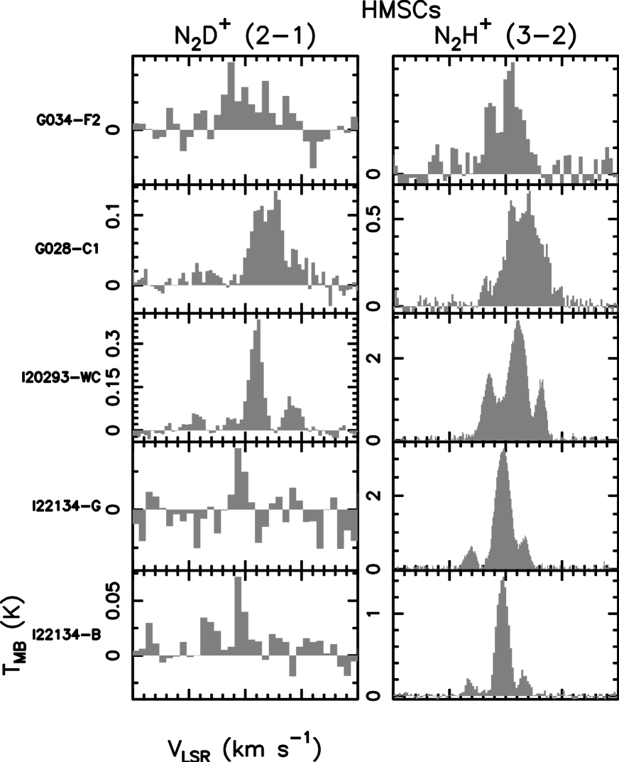
Figure B-2: Fig. B-1 continued.

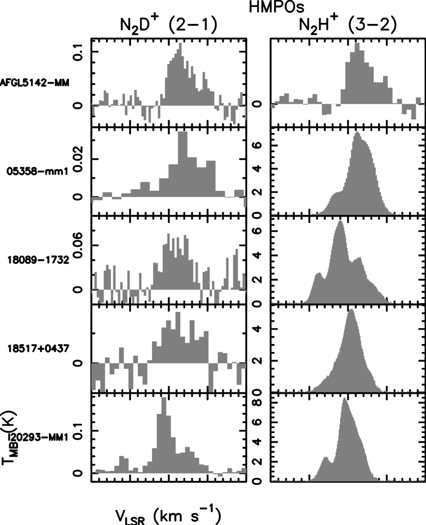
Figure B-3: Same as Fig B-1 for HMPOs.

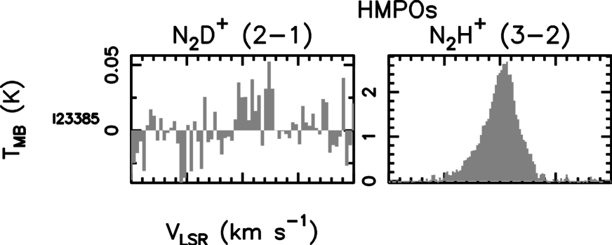
Figure B-4: Fig. B-3 continued.

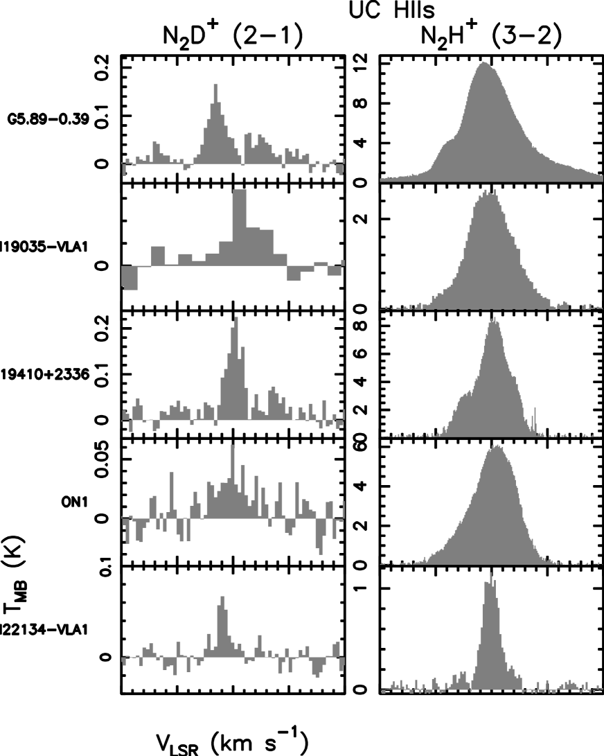
Figure B-5: Same as Fig. B-1 for UC HII regions.

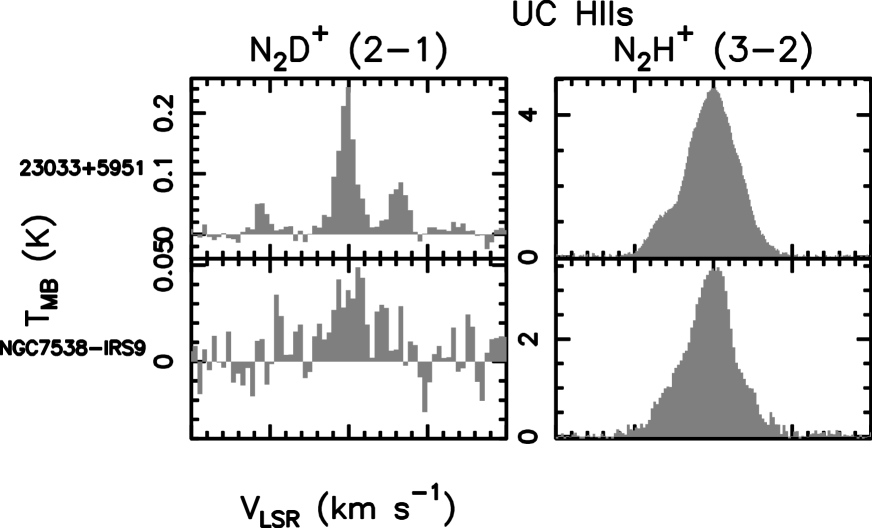
Figure B-6: Fig. B-5 continued.

References

- Aikawa et al. (2005) Aikawa, Y., Herbst, E., Roberts, H., Caselli, P. 2005, ApJ, 620, 330
- Ando et al. (2011) Ando, K., Nagayama, T., Omodaka, T. et al. 2011, accepted for publication in PASJ, arXiv:1012.5715
- Beuther et al. (2007a) Beuther, H., Churchwell, E.B., McKee, C.F., Tan, J.C. 2007, PPV, B. Reipurth, D. Jewitt, and K. Keil (eds.), University of Arizona Press, Tucson, p. 165
- Beuther et al. (2007b) Beuther, H., Leurini, S., Schilke, P. et al. 2007, A&A, 466, 1065
- Beuther et al. (2004) Beuther, H., Hunter, T.R., Zhang, Q. et al. 2004, ApJ, 616, L23
- Beuther et al. (2002) Beuther, H., Walsh, A., Schilke, P. et al. 2002, A&A, 390, 289
- Busquet et al. (2011) Busquet, G., Estalella, R., Zhang et al. 2011, A&A, 525, A141
- Busquet (2010) Busquet, G. 2010, PhD Thesis, University of Barcelona
- Busquet et al. (2010) Busquet, G., Palau, A., Estalella, R. et al. 2010, A&A, 517, L6
- Butler & Tan (2009) Butler, M.J. &Tan, J.C. 2009, ApJ, 696, 484
- Caselli et al. (2008) Caselli, P., Vastel, C., Ceccarelli, C. et al. 2008, A&A, 492, 703
- Caselli (2002a) Caselli, P. 2002a, P&SS, 50, 1133
- Caselli et al. (2002b) Caselli, P., Walmsley C.M., Zucconi, A. et al. 2002a, ApJ, 565, 331
- Caselli et al. (2002c) Caselli, P., Walmsley C.M., Zucconi, A. et al. 2002b, ApJ, 565, 344
- Chen et al. (2010) Chen, H.-R., Liu, S.-Y., Su, Y.-N., Zhang, Q. 2010, ApJ, 713, L50
- Crapsi et al. (2005) Crapsi, A., Caselli, P., Walmsley, C.M., et al. 2005, ApJ, 619, 379
- Emprechtinger et al. (2009) Emprechtinger, M., Caselli, P., Volgenau, N.H., Stutzki, J., Wiedner, M.C. 2009, A&A, 493, 89
- Fontani et al. (2009) Fontani, F., Zhang, Q., Caselli, P., Bourke, T.L. 2009, A&A, 499, 233
- Fontani et al. (2006) Fontani, F., Caselli, P., Crapsi, A. et al. 2006, A&A, 460, 709
- Fontani et al. (2004a) Fontani, F., Cesaroni, R., Testi, L. et al. 2004a, A&A, 424, 179
- Fontani et al. (2004b) Fontani, F., Cesaroni, R., Testi, L. et al. 2004b, A&A, 414, 299
- Foster et al. (2009) Foster, J.B., Rosolowsky, E.W., Kauffmann, J. 2009, ApJ, 696, 298
- Friesen et al. (2010) Friesen, R.K., Di Francesco, J., Myers, O.C. 2010, ApJ, 718, 666
- Ginsburg et al. (2009) Ginsburg, A.G., Bally, J., Yan, C.-H., Williams, J.P. 2009, ApJ, 707, 310
- Hunter et al. (2008) Hunter, T.R., Brogan, C.L., Indebetouw, R., Cyganowski, C. 2008, ApJ, 680, 1271
- Jijina et al. (1999) Jijina, J., Myers, P.C., Adams, F.C. 1999, ApJS, 125, 161
- Kutner & Ulich (1981) Kutner, M.L. & Ulich, B.L. 1981, ApJ, 250, 341
- Millar et al. (1989) Millar, T.J., Bennett, A., Herbst, E. 1989, ApJ, 340, 906
- Molinari et al. (1996) Molinari, S., Brand, J., Cesaroni, R., Palla, F. 1996, A&A, 308, 573
- Motogi et al. (2011) Motogi, K., Sorai, K., Habe, A. et al. 2011, accepted for publication in PASJ, arXiv:1012.4248
- Nagayama et al. (2011) Nagayama, T., Omodaka, T., Nakagawa, A. et al. 2011, accepted for publication in PASJ, arXiv:1012.5711
- Oliveira et al. (2003) Oliveira, C.M., Hébrard, G., Howk, J.C. et al. 2003, ApJ, 587, 235
- Pagani et al. (2007) Pagani, L., Bacmann, A., Cabrit, S., Vastel, S. 2007, A&A, 467, 179
- Palau et al. (2010) Palau, A., Sánchez-Monge, Á., Busquet, G. et al. 2010, A&A, 510, 5
- Palau et al. (2007) Palau, A., Estalella, R., Girart, J.M. et al. 2007, A&A, 465, 219
- Pillai et al. (2007) Pillai, T., Wyrowski, F.; Hatchell, J.; Gibb, A. G.; Thompson, M. A. 2007, A&A, 467, 207
- Pillai et al. (2006) Pillai, T., Wyrowski, F., Carey, S.J., Menten, K.M. 2006, A&A, 450, 569
- Rathborne et al. (2010) Rathborne, J.M., Jackson, J.M., Chambers, E.T. et al. 2010, ApJ, 715, 310
- Sánchez-Monge (2011) Sánchez-Monge, Á. 2011, PhD Thesis, University of Barcelona
- Sánchez-Monge et al. (2008) Sánchez-Monge, Á., Palau, A., Estalella, R., Beltrán, M.T., Girart, J.M. 2008, A&A, 485, 497
- Schnee & Carpenter (2009) Schnee, S. & Carpenter, J. 2009, ApJ, 698, 1456
- Sridharan et al. (2002) Sridharan, T.K., Beuther, H., Saito, M., Wyrowski, F., Schilke, P. 2005, ApJL, 634, 57
- Su et al. (2009) Su, Y.-N., Liu, S.-Y., Lim, J. 2009, ApJ, 698, 1981
- Tiné et al. (2004) Tafalla, M., Myers, P.C., Caselli, P., Walmsley, C.M. 2004, A&A, 416, 191
- Zhang et al. (2002) Zhang, Q., Hunter, T.R., Sridharan, T.K.; Ho, P.T.P. 2002, ApJ, 566, 982
- Zinnecker & Yorke (2007) Zinnecker, H. & Yorke, H.W. 2007, ARA&A, 45, 481