E, B, $\mu$, T Phase Structure of the D3/D7 Holographic Dual

Abstract

The large $N$ ${\cal N}$=4 gauge theory with quenched ${\cal N}$=2 quark matter displays chiral symmetry breaking in the presence of a magnetic field. We previously studied the temperature and chemical potential phase structure of this theory in the grand canonical ensemble - here we, in addition, include the effect of an electric field which acts to counter chiral symmetry breaking by disassociating mesons. We compute using the gravity dual based on the D3/probe-D7 brane system. The theory displays two transition at one of which chiral symmetry is restored. At the other transition density switches on, the mesons of the theory become unstable and a current forms, making it a conductor-insulator transition. Through the temperature, electric field, chemical potential volume (at fixed magnetic field parallel to the electric field) these transitions can coincide or separate at critical points, and be first order or second order. We map out this full phase structure which provides varied computable examples relevant to strongly coupled gauge theories and potentially condensed matter systems.

1 Introduction and summary

Holographic techniques Malda ; Witten:1998qj ; Gubser:1998bc have begun to allow us to study the phase structure of strongly coupled gauge theories. Such studies are potentially of interest for QCD, more exotic gauge theories and even to condensed matter systems. Although it is somewhat hard to dial a particular gauge theory, we instead work in tractable models that lie close to ${\cal N}=4$ Super Yang-Mills theory and hope that these gauge theories show similar behaviours to realistic cases.

A simple model to study is the large $N$ ${\cal N}=2$ gauge theory made from ${\cal N}=4$ SYM plus a small number of quark hypermultiplets Karch ; Polchinski ; Bertolini:2001qa ; Mateos ; Erdmenger:2007cm . In the limit $N_{f}\ll N$ quark loops are quenched which on the gravity side implies that one can study probe D7 (or D5) branes in the AdS background of $N$ D3 branes. In the presence of a magnetic field ($B$) the theory dynamically generates a quark condensate that breaks a chiral $U(1)$ global symmetry Johnson1 . This dynamics may be relevant to condensed matter systems Evans2 ; Jensen ; Evans3 but one can also study it as a loose analogue of QCD-like gauge theories Evans1 . Of course in those theories the running coupling generates a scale and the chiral symmetry breaking, but the hard magnetic field can be thought of as the analogue of the scale $\Lambda_{QCD}$ which breaks the conformal symmetry and “allows” the strong dynamics to generate a condensate ($c$).

In Evans1 we computed the phase diagram for the theory with massless quarks, in a magnetic field, in the temperature chemical potential plane ($T$-$\mu$ plane) which we show in Fig 1(a). It has considerable structure. Whilst the magnetic field favours chiral symmetry breaking the temperature Babington and chemical potential Myers1 favour the chirally symmetric phase. This tension leads to interesting phase structure. There are three phases - the high $T$, $\mu$ phase with the symmetry restored ($\chi$S), finite density ($d\neq 0$) and no stable mesonic states; an intermediate phase in which chiral symmetry is broken ($\chi$SB), finite density ($d\neq 0$), but mesons are still unstable; and finally a low $T$, $\mu$ phase with broken chiral symmetry ($\chi$SB), no density ($d=0$) and stable mesons. On the gravity side these phases are described by a flat D7 embedding, an embedding that spikes on to the black hole horizon, and a solution that lies outside the horizon (See the insets in Fig 1(a) for schematic plots.). These phases are linked by transition lines that are in places first order (blue lines) and in places second order (red lines) - critical points link these behaviours. Time dependent aspects of these transitions have also been studied in Evans4 ; Grosse:2007ty ; Guralnik:2011xz ; Evans5 .

In this paper we wish to study how robust the phase structure is to changes of parameters. In particular we will introduce the additional parameter of an electric field ($E$) parallel to the magnetic field. Note this case is simpler than when the $E$ and $B$ fields are perpendicular because no Hall current forms. We do allow for the induced current in the direction of the electric field. The effect on the theory of an electric field has been studied previously for probe branes in Andy1 ; Hall ; Erdmenger1 ; Veselin1 ; Andy2 ; Mas ; Andy3 . Although the electric field continuously acts on the quarks an equilibrium configuration is nevertheless reached where energy is being dissipated to the bulk ${\cal N}=4$ plasma. The quarks and anti-quarks have opposite charge when interacting with the electric field so the field tends to loosen the binding in mesonic bound states and, if it is strong enough, to disassociate the mesons. With an electric field present in the theory a singular shell develops in the gravity description. If the D7 brane passes through this shell its action becomes imaginary and in order to keep the action real one must turn on the appropriate electric current ($J$). The singular shell plays the role of an effective horizon for world volume meson fluctuations KST . If the probe brane touches the singular shell one expects that fluctuations of the brane there must be in-falling and the spectrum will resemble a quasi-normal mode spectrum describing mesons that have a complex mass. In other words the electric field has acted to disassociate the meson in a similar fashion to how temperature melts the mesons Peeters:2006iu .

The field theory phase structure is determined holographically by comparison of the classical bulk field configurations. In this paper, we introduce three bulk fields $L(\rho)$ (embedding scalar), $A_{t}(\rho)$ (gauge field), and $A_{x}(\rho)$ (gauge field) in the D7 brane world volume with given background parameters ($E,B,T$). By fixing the asymptotic values of fields in the UV (large $\rho$) as ($L\rightarrow m$ (quark mass), $A_{t}\rightarrow\mu$ (chemical potential), $A_{x}\rightarrow 0$), we look for the sub-leading behaviors of fields at large $\rho$: $c$ (condensate), $d$ (density), and $J$ (current), which are determined by the bulk DBI dynamics. Therefore, our problem is classifying the phases by three quantities $(c,d,J)$ in the 5D space ($T,B,E,m,\mu$). It turns out that, because of a scaling symmetry, we can scale all variables by $B$, which reduces our phase space to 4D. Since we are interested in spontaneous chiral symmetry breaking, we will choose $m=0$. Our phase space becomes 3D ($T,\mu,E$) and we will classify this space by 8 possible states consisting of the three order parameters ($c,d,J$) being “on or off”. Among them, only in the $c\neq 0,d=J=0$ phase are stable mesons allowed. $T,\mu,E$ tend to turn off $c$ ($c=0$) and turn on $d,J$ ($d,J\neq 0$), and so oppose $B$. Due to these competitions between $E,T,\mu$ and $B$ a rich phase structure is constructed.

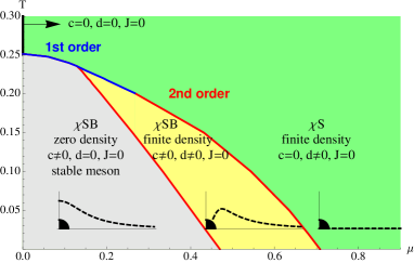
(a) $T$-$\mu$ phase diagram. The inset diagrams are representative probe brane embeddings (dotted lines), where a black disk represents a black hole.

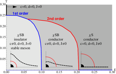
(b) $T$-$E$ phase diagram. The inset diagrams are representative probe brane embeddings (dotted lines), where a red arc represents a singular shell.

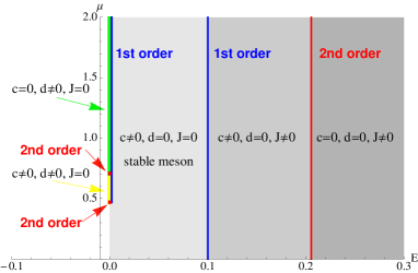
(c) $\mu$-$E$ phase diagram. The $\mu$($E$) axis agrees with the $\mu$($E$) axis of Fig 1(a)(1(b)) and are shown by the same color. Thus embeddings are the same as 1(a) and 1(b) without the black hole.

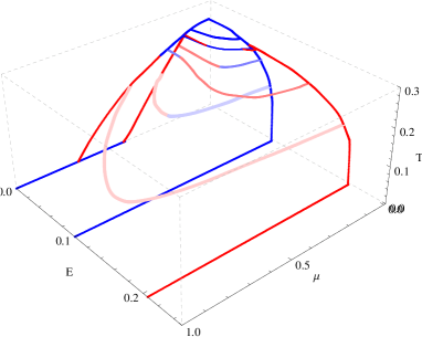
(d) $E$-$\mu$-$T$ phase diagram. The curves show the phase boundaries at fixed $T$ ($T=0$, $0.15$, $0.21$, $0.232$, $0.24$ from the bottom). See Fig 7 for more detail.

Figure 1: The phase diagrams of the massless ${\cal N}=2$ gauge theory with a magnetic field. First order transitions are shown in blue, second order transitions in red. The temperature is controlled by the parameter $T$, chemical potential by $\mu$ and electric field by $E$.

One of our main results here is that three phases (corresponding to three embedding types) are also present in the $T,E$ plane as we summarize in Fig 1(b). With a large (small) electric field, the theory becomes a conductor (insulator) and is in $\chi$S ($\chi$SB) phase. At an intermediate electric field, the system is a chiral symmetry broken conductor. Note that the orders of the phase transitions and the positions and presence of the critical points vary relative to the $T,\mu$ case (Fig 1(a)).

Interestingly, the $\mu$-$E$ phase diagram (Fig 1(c)) shows a very different structure from the $T$-$\mu$ or the $T$-$E$ phase diagram. At zero temperature and finite $E$ and $B$ field, the contribution to the action from the density is canceled by the contribution from the induced current, which is a function of density. Consequently the free energy of the system is independent of density, which was pointed out in Erdmenger1 in the zero $B$ field case. Thus the system is essentially a zero density system and the phase diagram is independent of the chemical potential. At first this may seem at odds with Fig 1(a) since the $\mu$ axis has structure present. In fact there is a first order transition at $T=0$ between the $\mu$ axis and the rest of the $E,\mu$ plane. There are two limits approaching the $\mu$-axis: (1) $E=0$ and then $T\rightarrow 0$ (2) $T=0$ and then $E\rightarrow 0$. These two limits are different and only the former is a continuous limit to the $\mu$-axis.

Indeed by computing the phase structure through the entire $T,\mu,E$ volume (e.g. computing the $\mu$-$E$ diagram at various fixed $T$) we show the smooth evolution through that volume connecting the three surface planes. There are interesting movements of the critical points and phase boundaries. These results are summarized in Fig 1(d) which we discuss in much more detail in section 6. We also see the development of the first order transition between the $E$-$\mu$ plane and the $\mu$-axis as $T\rightarrow 0$. Two of the missing states from Fig 1(a)-1(c), ($c\neq 0,d\neq 0,J\neq 0$) and ($c=0,d\neq 0,J\neq 0$) from among the 8 possible states, are found in the 3D bulk of Fig 1(d).

These models with their varied behaviours in the $B,T,\mu,E$ volume can hopefully serve as exemplars, or templates from which to find exemplars, for different phase structures in physical theories.

2 The holographic description

The ${\cal N}$=4 gauge theory at finite temperature has a holographic description in terms of an AdS₅ black hole geometry (with $N$ D3 branes at its core)Malda ; Witten:1998qj ; Gubser:1998bc . The geometry is

$$ds^{2}=\frac{r^{2}}{R^{2}}(-fdt^{2}+d\vec{x}^{2})+\frac{R^{2}}{r^{2}f}dr^{2}+R^{2}d\Omega_{5}^{2}\ ,$$ (1)

where $R^{4}=4\pi g_{s}N\alpha^{{}^{\prime}2}$ and

$$f:=1-\frac{r_{H}^{4}}{r^{4}}\ ,\qquad r_{H}:=\pi R^{2}T_{\mathrm{FT}}\ .$$ (2)

Here $r_{H}$ is the position of the black hole horizon which is linearly related to the dual field theory temperature $T_{\mathrm{FT}}$.

We will find it useful to make the coordinate transformation

$$\frac{dr^{2}}{r^{2}f}\equiv\frac{dw^{2}}{w^{2}}\ \Longrightarrow\ \sqrt{2}w:=\sqrt{r^{2}+\sqrt{r^{4}-r_{H}^{4}}}\ ,$$ (3)

with $\sqrt{2}w_{H}=r_{H}$. This change makes the presence of a flat 6-plane perpendicular to the horizon manifest. We will then write the coordinates in that plane as $\rho$ and $L$ according to

$$w=\sqrt{\rho^{2}+L^{2}}\ ,\quad\rho:=w\sin\theta\ .\quad L:=w\cos\theta\ ,$$ (4)

The metric is then

$$ds^{2}=\frac{w^{2}}{R^{2}}(-g_{t}dt^{2}+g_{x}d\vec{x}^{2})+\frac{R^{2}}{w^{2}}(d\rho^{2}+\rho^{2}d\Omega_{3}^{2}+dL^{2}+L^{2}d\Omega_{1}^{2})\ ,$$ (5)

where

$$g_{t}:=\frac{(w^{4}-w_{H}^{4})^{2}}{w^{4}(w^{4}+w_{H}^{4})}\ ,\qquad g_{x}:=\frac{w^{4}+w_{H}^{4}}{w^{4}}\ .$$ (6)

Quenched ($N_{f}\ll N$) ${\cal N}$=2 quark superfields can be included in the ${\cal N}$=4 gauge theory through probe D7 branes in the geometryKarch ; Polchinski ; Bertolini:2001qa ; Mateos . The D3-D7 strings are the quarks. D7-D7 strings holographically describe mesonic operators and their sources. The D7 probe can be described by its DBI action

$$S_{DBI}=-T_{D7}\int d^{8}\xi\sqrt{-{\rm det}(P[G]_{ab}+2\pi\alpha^{\prime}F_{ab})}\ ,$$ (7)

where $P[G]_{ab}$ is the pullback of the metric and $F_{ab}$ is the gauge field living on the D7 world volume. We will use $F_{ab}$ to introduce a constant magnetic field (eg $F_{12}=-F_{21}=B/(2\pi\alpha^{\prime})$) Johnson1 , a chemical potential associated with baryon number $A_{t}(\rho)\neq 0$ Myers1 ; Kim and our crucial extra ingredient here an electric field parallel to the magnetic field ($F_{03}=-F_{30}=E/(2\pi\alpha^{\prime})$)Andy1 ; Hall ; Erdmenger1 ; Veselin1 . We will also allow for the possibility that the electric field induces a current in the $z$-direction by including $A_{z}$.

We embed the D7 brane in the $t$, $\vec{x}$, $\rho$ and $\Omega_{3}$ directions of the metric but to allow all possible embeddings must include a profile $L(\rho)$ at constant $\Omega_{1}$. The full DBI action we will consider is then

$$S=\int d\xi^{8}\mbox{${\cal L}$}(\rho)=\left(\int_{S^{3}}\epsilon_{3}\int dtd\vec{x}\right)\int d\rho\ \mbox{${\cal L}$}(\rho)\ ,$$ (8)

where $\epsilon_{3}$ is a volume form on the 3-sphere. Here

$${\cal L} := -\mbox{${\cal N}$}\rho^{3}\left(1-\frac{w_{H}^{4}}{w^{4}}\right)\sqrt{\left(\left(1+\frac{w_{H}^{4}}{w^{4}}\right)^{2}+\frac{R^{4}}{w^{4}}B^{2}\right)}$$

$$\times\sqrt{\left(\left(1-\frac{E^{2}R^{4}w^{4}}{(w^{4}-w_{H}^{4})^{2}}\right)(1+L^{\prime 2})-\frac{w^{4}(w^{4}+w_{H}^{4})}{(w^{4}-w_{H}^{4})^{2}}(2\pi\alpha^{\prime}A_{t}^{\prime})^{2}+\frac{w^{4}}{w^{4}+w_{H}^{4}}(2\pi\alpha^{\prime}A_{z}^{\prime})^{2}\right)}\ ,$$

and $\mbox{${\cal N}$}:=N_{f}T_{D7}$. At large $\rho$, for fixed $E$ and $B$, the fields behave as

$$L\sim m+{c\over\rho^{2}}+...,\hskip 14.22636ptA_{t}\sim\mu+{d\over\rho^{2}}+...,\hskip 14.22636ptA_{z}\sim{J\over\rho^{2}}\ ,$$ (10)

where $m$ is the quark mass, $c$ the quark condensate, $\mu$ the chemical potential, $d$ the quark density and $J$ the current. Since the action is independent of $A_{t}$ and $A_{z}$, there are conserved quantities $d$ $\left(:=\frac{\delta S}{\delta F_{\rho t}}\right)$ and $J$ $\left(:=\frac{\delta S}{\delta F_{\rho z}}\right)$. These relations can be inverted to express $A_{t}^{\prime}$ and $A_{z}^{\prime}$ in terms of $d$ and $J$ as

$$2\pi\alpha^{\prime}A_{t}^{\prime}=\frac{d}{2\pi\alpha^{\prime}\mbox{${\cal N}$}}\frac{w^{4}-w_{H}^{4}}{w^{4}+w_{H}^{4}}Q\ ,\qquad 2\pi\alpha^{\prime}A_{z}^{\prime}=\frac{J}{2\pi\alpha^{\prime}\mbox{${\cal N}$}}\frac{w^{4}+w_{H}^{4}}{w^{4}-w_{H}^{4}}Q\ ,$$ (11)

$$Q:=\sqrt{\frac{\left(1-E^{2}R^{4}\frac{w^{4}}{(w^{4}-w_{H}^{4})^{2}}\right)(1+L^{\prime 2})}{\left(\frac{d}{2\pi\alpha^{\prime}\mbox{${\cal N}$}}\right)^{2}\frac{w^{4}}{(w^{4}+w_{H}^{4})}-\left(\frac{J}{2\pi\alpha^{\prime}\mbox{${\cal N}$}}\right)^{2}\frac{w^{4}(w^{4}+w_{H}^{4})}{(w^{4}-w_{H}^{4})^{2}}+\left(\frac{B^{2}R^{4}}{w^{4}}+\left(1+\frac{w_{H}^{4}}{w^{4}}\right)^{2}\right)\rho^{6}}}\ .$$

This is used to express the Legendre transformed action in terms of $d$ and $J$:

$$S_{LT} = S-\int d\xi^{8}F_{\rho t}\frac{\delta S}{\delta F_{\rho t}}-\int d\xi^{8}F_{\rho z}\frac{\delta S}{\delta F_{\rho z}}$$ (12)

$$= \left(\int_{S^{3}}\epsilon_{3}\int dtd\vec{x}\right)\int d\rho\ {\mbox{${\cal L}$}_{LT}}(\rho)\ ,$$

where

$$\mbox{${\cal L}$}_{LT} := -\mbox{${\cal N}$}\frac{(w^{4}-w_{H}^{4})}{w^{4}}\sqrt{K(1+L^{\prime 2})}\ ,$$ (13)

$$K := \left(1-\frac{E^{2}R^{4}w^{4}}{(w^{4}-w_{H}^{4})^{2}}\right)\left[\left(\frac{w^{4}+w_{H}^{4}}{w^{4}}\right)^{2}\rho^{6}+\frac{R^{4}B^{2}}{w^{4}}\rho^{6}\right.$$ (14)

$$\left.\hskip 28.45274pt+\frac{w^{4}}{(w^{4}+w_{H}^{4})}\frac{d^{2}}{(N_{f}T_{D7}2\pi\alpha^{\prime})^{2}}-\frac{w^{4}(w^{4}+w_{H}^{4})}{(w^{4}-w_{H}^{4})^{2}}\frac{J^{2}}{(N_{f}T_{D7}2\pi\alpha^{\prime})^{2}}\right]\ .$$

Note that the first factor of $K$ changes sign at $w_{s}$,

$$w_{s}=\sqrt{\frac{ER^{2}}{2}+\frac{\sqrt{E^{2}R^{4}+4w_{H}^{4}}}{2}}\ ,$$ (15)

which defines a singular shell with a radius $w_{s}$. At zero temperature ($w_{H}=0$) the singular shell forms at $\sqrt{E}R$, and at zero $E$, it merges into the horizon $w_{s}=w_{H}$. Note that the singular shell does not depend on density. In order to make the action regular, the second term of $K$ should change sign at the singular shell. This condition determines the current $J$ and conductivity $\sigma$ by Ohm’s law:

$$J=\sigma E\ ,$$ (16)

$$\sigma:=\mbox{${\cal N}$}(2\pi\alpha^{\prime})R^{2}\sqrt{\frac{w_{s}^{4}}{(w_{s}^{4}+w_{H}^{4})^{2}}\frac{d^{2}}{N^{2}(2\pi\alpha^{\prime})^{2}}+\left[\frac{R^{4}}{w_{s}^{4}(w_{s}^{4}+w_{H}^{4})}B^{2}+\frac{(w_{s}^{4}+w_{H}^{4})}{w_{s}^{8}}\right]\rho_{s}^{6}}\ ,$$

where $\rho_{s}$ is the $\rho$ coordinate where an embedding touches the singular shell. This is still a function of quark mass $m$ after all other parameters are fixed. Inspite of the way we write (16) the current is non linear in $E$ since $w_{s}$ and $\rho_{s}$ are functions of $E$. $\sigma$ has two contributions. The first term is from net charge carrier density, $d$, and the second term is from pair produced virtual charges. Interestingly, the conductivity by pair produced charges are enhanced by $B$. The more general conductivity for arbitrarily angled constant $E$ and $B$ was obtained in Hall ; Andy3 in a different coordinate system. By plugging (16) into (13) and rescaling we have a dimensionless Lagrangian $\widetilde{\mbox{${\cal L}$}}_{LT}$:

$$\widetilde{\mbox{${\cal L}$}}_{LT}:=-\frac{\mbox{${\cal L}$}_{LT}}{R^{4}B^{2}\mbox{${\cal N}$}}=\frac{(w^{4}-T^{4})}{w^{4}}\sqrt{\widetilde{K}(1+L^{\prime 2})}\ ,$$ (17)

$$\widetilde{K}:=\left(1-\frac{E^{2}w^{4}}{(w^{4}-T^{4})^{2}}\right)\left[\left(\frac{w^{4}+T^{4}}{w^{4}}\right)^{2}\rho^{6}+\frac{1}{w^{4}}\rho^{6}+d^{2}\frac{w^{4}}{(w^{4}+T^{4})}\right.$$

$$\left.\hskip 28.45274pt-E^{2}\frac{w^{4}(w^{4}+T^{4})(w_{s}^{4}+(w_{s}^{4}+T^{4})^{2})}{(w^{4}-T^{4})^{2}(w_{s}^{4}+T^{4})w_{s}^{8}}\rho_{s}^{6}-d^{2}E^{2}\frac{w^{4}(w^{4}+T^{4})w_{s}^{4}}{(w^{4}-T^{4})^{2}(T^{4}+w_{s}^{4})^{2}}\right]\ ,$$ (18)

where we rescaled

$$(\omega,L,\rho)\rightarrow R\sqrt{B}\ (\omega,L,\rho)\ ,\quad(d,J)\rightarrow(R\sqrt{B})^{3}\mbox{${\cal N}$}2\pi\alpha^{\prime}\ (d,J)\ ,\quad E\rightarrow BE\ ,$$ (19)

and define $T\equiv w_{H}$ for notational clarity. The Lagrangian $\widetilde{\mbox{${\cal L}$}}_{LT}$ will be our starting point for the numerical analysis in the following sections.

The chemical potential is obtained by integrating $A_{t}^{\prime}$ (11) from the horizon to the boundary

$$\mu=\int_{\rho_{H}}^{\infty}d\frac{w^{4}-T^{4}}{w^{4}+T^{4}}\sqrt{\frac{\left(1-E^{2}\frac{w^{4}}{(w^{4}-T^{4})^{2}}\right)(1+L^{\prime 2})}{d^{2}\frac{w^{4}}{(w^{4}+T^{4})}-J^{2}\frac{w^{4}(w^{4}+T^{4})}{(w^{4}-T^{4})^{2}}+\left(\frac{1}{w^{4}}+\left(1+\frac{T^{4}}{w^{4}}\right)^{2}\right)\rho^{6}}}\ ,$$ (20)

where $A_{t}(\rho_{H})=0$.

In the following sections we will present our results on various aspects of the phase structure of this theory. Until the final section we will concentrate on the case of massless quarks where the $U(1)$ symmetry in the $d\Omega_{1}$ direction is a good UV symmetry of the theory. Also here and below we will express all our dimensionful parameters in units of the magnetic field $B$ to the appropriate power (see (19)) - in other words we will use the magnetic field as the intrinsic scale in the theory.

3 $B$, $T$, $\mu$ Phase Diagram

In this section we review previous results Evans1 on the theory without an electric field present. The influence of $B$, $\mu$ and $T$ on the D7 embedding can be understood qualitatively as follows. With none of these terms present the embedding of the ${\cal N}=2$ theory for massless quarks is just flat, $L(\rho)=0$ - $c$ is zero and there is no quark condensate generated to break the $U(1)$ symmetry.

Temperature is represented by an attractive black hole at small $\rho$ and also favours a flat embedding. The presence of density $d$ leads to solutions that spike to the origin (or on to the black hole horizon with temperature present) - the spike can be thought of as strings linking the D3 and D7 branes and represent the density of quarks explicitly. Note that at finite chemical potential there can also be solutions with $A_{t}=\mu$ and $d=0$ - the action for such solutions is independent of $\mu$ and hence so are the embeddings.

Non-trivial embeddings are generated by the $B$ field. We can see from (2) that the last square root term grows if the embedding approaches $w=0$ when there is a $B$ field. The embeddings tend to curve off axis to avoid the origin leading to a non-zero quark condensate $c$ and spontaneous breaking of the $U(1)$ symmetry.

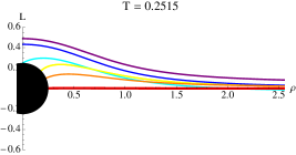
(a) The D7 brane embeddings

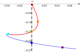
(b) $m$- $c$ diagrams

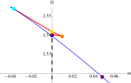
(c) the Free energies

Figure 2: Exemplary plots in the presence of a magnetic field at finite chemical potential and with temperature $T=0.2156$. (Parameters are scaled by $B$.)

The interesting phase structure of the theory is generated by the competition between the $B$ field wanting to break the $U(1)$ symmetry and $d$ and $T$ which seek to restore it. As an example we show in Fig 2(a) solutions of the Euler-lagrange equations for the embedding for a case with $\sqrt{B}>T>\mu$ - the red embedding is flat and preserves the symmetry, the yellow embedding spikes on to the horizon and the dark blue embedding breaks the $U(1)$ symmetry and has $d=0$. The full phase diagram is generated by competition between these three types of embeddings.

To decide which of the embeddings represents the true vacuum one may compute the free energy $\Omega=-S$ evaluated on the solutions. This plot is shown on the right hand side of Fig 2(c). Here we see that we have chosen a transition point where the red and dark blue curves are degenerate - for larger $T$ the flat embedding is preferred. Here this transition is associated with chiral symmetry restoration ($c$ changes from non-zero to zero) and melting of the mesonic degrees of freedom (the brane moves from off the horizon to on it). It is a first order transition.

The transition’s presence and position in parameter space can also be seen from the middle plot in Fig 2(b). Here we plot the condensate $c$ against the quark mass $m$. To obtain this plot we must find solutions for the embeddings that lie off axis as $\rho\rightarrow\infty$ such as the green and orange curves shown. We can see the presence of the three solutions discussed at $m=0$ in the middle plot. To see there is a phase transition at this point we can use a Maxwell construction. The quark mass and condensate are conjugate variables and therefore the area between the $c$ axis and the curve represents the free energy difference between two points on the curve. At this point the two segments of the curve generate equal area and the first order transition between the red and blue points is predicted.

In Evans1 we fleshed out in this way the full phase diagram of the theory which we show in Fig 1(a). We quickly present the results here since the analysis is a subset of the work in section 6 below. In the bottom left segment the symmetry breaking, black hole avoiding embedding is the vacuum; in the central section a spike embedding is preferred; and to the right the symmetry preserving flat embedding is the vacuum. The low $T,\mu$ phase has chiral symmetry breaking, no density and stable meson states; the central regime chiral symmetry breaking, finite density and melted mesons; in the high $T,\mu$ phase the symmetry is restored and the mesons melted at finite density. The order of the transitions is marked as well and each transition has periods where it is first and second order, linked by critical points.

4 $B$, $T$, $E$ Phase Diagram

The rich structure of the $B,\mu,T$ phase diagram leads one to ask how generic it is? The main goal of this paper is to introduce an additional parameter that favours chiral symmetry preservation to see how sensitive the phase diagram is to a change of parameter. We will use electric field ($E$) as that new parameter.

4.1 $B$, $E$ at zero temperature

As a first example lets consider the system with $E$ and $B$ but no $T$ or $\mu$. The Legendre transformed Lagrangian is

$$\widetilde{\mbox{${\cal L}$}}_{LT}=\sqrt{(1+L^{\prime 2})}\sqrt{\left(1-\frac{E^{2}}{w^{4}}\right)\left[\rho^{6}+\frac{\rho^{6}}{w^{4}}-J^{2}\right]}\ .$$ (21)

As has been discussed in (15) and (16), there is a singular shell at $w_{s}=\sqrt{E}$ and the current is given by

$$J=E\frac{\sqrt{1+w_{s}^{4}}\rho_{s}^{3}}{w_{s}^{4}}=\sqrt{(1+E^{2})E\cos^{6}\theta_{s}}\ .$$ (22)

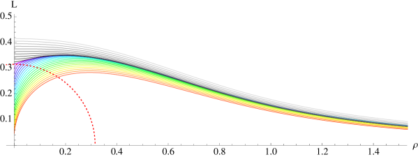
(a) Embeddings ending on and off the singular shell ($E=0.1,m=0$).

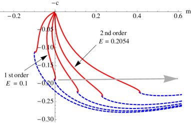
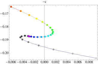
(b) The condensate, $c$ vs mass, $m$ for given $E$ values. Curves shift to left as $E$ decreases. The red (blue) part corresponds to the embedding touching (missing) the singular shell. The inset on the right is a zoom-in around the first order phase transition. The colored points correspond to the colored embeddings in Fig 3(a).

Figure 3: Embeddings and $c$-$m$ diagram at finite $E$ parallel to finite $B$, but no density and temperature.

One can therefore find the embeddings that end on the singular shell by shooting out (in) from the singular shell with $J$ determined by the point on the shell one is shooting from. We then seek amongst such solutions for those that satisfy $L\rightarrow 0$ ($m\rightarrow 0$) as $\rho\rightarrow\infty$ to find the massless (mass $m$) embeddings. Generically we again find three types of solutions - (1) embeddings that curve off axis and reach $\rho=0$ missing the singular shell (when $E\ll B$); (2) embeddings that curve off axis and pass through the singular shell (when $E\sim B$); (3) the flat embedding $L=0$. The schematic plots of these three cases are shown in the inset of Fig 1(b), where the black disk should be ignored at zero $T$. In Fig 3(a) we show some sample numerical embeddings ending on (2) and off (1) the singular shell.

All non-flat embeddings that pass through the singular shell have a conical singularity at $\rho=0$, whose precise interpretation is unclear and discussed in Erdmenger1 ; Veselin1 . The conical singularity is most likely a reflection of the energy being injected by the electric field being sunk into the gauge background through stringy physics representing the quark interactions with the ${\cal N}=4$ Yang-Mills fields.

The Fig 3(b) shows the condensate, $c$, vs mass, $m$, plot for given $E$s. One point ($c$,$m$) in the plot corresponds to one embedding since it gives a complete initial condition for the embedding equation (a second order differential equation). For example, the colored points in the inset of Fig 3(b) correspond to the embedding in Fig 3(a) of the same color.

From Fig 3(b) we can determine the phase structure as follows.

For a larger $E$ (relative to $B$), the $c$-$m$ curves tend to be pushed to the right. So if we focus on $m=0$ case, the only available point at large $E$ is $(m,c)=(0,0)$, which corresponds to the flat embedding. The flat embedding preserves the $U(1)$ chiral symmetry, so the system is chiral symmetric ($\chi$S). Since the flat embedding necessarily crosses the singular shell, there is no stable meson but there is a current (22) with $\theta_{s}=0$: $J=\sqrt{(1+E^{2})E}$, which is the maximal current for a given $E$. i.e. The system is a conductor.

As $E$ is lowered the $c$-$m$ curve shifts to the left. At $E\sim 0.2054$ a new solution for $m=0$ appears, whose $c$ is finite and the ground state corresponds to this new solution. This is a second order transition because the second solution for $c$ at $m=0$ moves smoothly away from the $c=0$ embedding. Because of the finite $c$, the embedding is curved and breaks the $U(1)$ symmetry, so the system is in a chiral symmetry broken ($\chi$SB) phase. However the embedding still passes through the singular shell, so it is a conductor with no stable meson.

Finally, around $E\sim 0.1$ the small ‘S’ shape structure connecting the red part (singular shell touching embedding) and blue part (a singular shell missing Minkowski embedding), meets the $m=0$ line, which is zoomed in, in the inset of Fig 3(b). It shows a typical first order phase transition structure and by a Maxwell construction we can pin down the transition point. So as $E$ decreases, the green point should move to the gray point with a discontinuous condensate jump (see the zoomed in inset). The blue part (or the gray points in the inset) corresponds to the Minkowski embedding and the system is a $\chi$SB insulator with stable mesons.

One would like to match this picture to a computation of the free energy. Naively it seems one should just compute the original action (before Legendre transforming) evaluated on these solutions. However, there is a subtle point related to the conical singularity of the embedding at $\rho=0$ and also a $\log$ divergence of $A_{x}$ Andy1 ; Andy2 ; Andy3 at the horizon. Thus we need to add some boundary term to take care of the singularity at $\rho=0$ or at the horizon. This boundary term will also contribute to the free energy so must be taken into account.

However, this surface term does not change the equation of motion. Furthermore, as far as the embedding dynamics is concerned, the singular shell position has the same singular structure as a black hole horizon and the embedding outside a singular shell is independent of the ones inside the shell. So the $c$-$m$ plots, based on the classical embedding outside the shell, are valid regardless of the additional boundary terms at the IR boundary.

These solutions correctly show us the maxima and minima of the free energy as a function of $E$. The discussion above is the only consistent picture with the $c$-$m$ plots so we can be confident of its validity. For this reason in what follows we will focus on the $c$-$m$ plots (and also when chemical potential is present we will track the quark density) to determine the phase structure. A similar philosophy was used in  Erdmenger1 ; Veselin1 .

However, it would be interesting to identify the correct boundary term and compute the consistent free energy graph for our $c$-$m$ plot (we have not been able to so far). To identify it, in principle, one should start with the time-dependent back-reacted system, since the singularities are related to time-dependent energy loss of the system and its effect on the background adjoint matters. However one may also be able to introduce an “effective” boundary term. Our $c$-$m$ diagram would be a good guide to figure out the correct boundary term and free energy or could even be used as a rule to determine it, since sometimes thermodynamic consistency plays a complementary role in AdS/CFT applications.

4.2 $B$, $E$ at finite temperature

We can now extend our analysis to include temperature straight forwardly. From (17) with $d=0$

$$\widetilde{\mbox{${\cal L}$}}_{LT}=\frac{(w^{4}-T^{4})}{w^{4}}\sqrt{\widetilde{K}(1+L^{\prime 2})},$$

$$\widetilde{K}=\left(1-\frac{E^{2}w^{4}}{(w^{4}-T^{4})^{2}}\right)\left[\left(\frac{w^{4}+T^{4}}{w^{4}}\right)^{2}\rho^{6}+\frac{1}{w^{4}}\rho^{6}-J^{2}\frac{w^{4}(w^{4}+T^{4})}{(w^{4}-T^{4})^{2}}\right]\ ,$$ (23)

and

$$w_{s}=\sqrt{\frac{E}{2}+\frac{\sqrt{E^{2}+4T^{4}}}{2}}\ ,\qquad J=E\sqrt{\frac{w_{s}^{4}+(w_{s}^{4}+T^{4})^{2}}{(w_{s}^{4}+T^{4})w_{s}^{8}}}\rho_{s}^{3}\ .$$ (24)

It is apparent that even with non-zero $T$ there remains a singular shell - it always lies outside $T$ for any $T$ (15). Requiring regularity of the onshell action allows us to fix the current $J$ (16). If the embedding does not touch the singular shell $\rho_{s}=0$, then there is no current.

We shoot out to obtain the embeddings as a function of $E$ and $T$ at fixed $B$. The process is laborious - we plot the evolution of the $c$-$m$ plot on fixed $T$ trajectories as we did at T=0 in the previous section. There are three types of $c$-$m$ plot. At low temperature, it is similar to Fig 3(b). At high temperature two qualitatively different structures appear as shown in Fig 4. As the temperature increases, the $T$ effect dominates the $E$ effect, which is visualized in the $c$-$m$ diagram as follows. The curve near $(m,c)=(0,0)$ is curved to the left (Fig 3(b)) at low $T$ but curved to the right (Fig 4(a)) at high $T$ (similarly to Fig 2), showing competition between $E$ and $T$. Both are an attractive effect from the embedding dynamic’s point of view, but the $T$ driven 1st order attraction is so strong that the $E$ driven 2nd order smooth attractive effect cannot be realized. At very high $T$ the repulsive effect of $B$ is completely suppressed and the only allowed embedding is a flat one (Fig 4(b)).

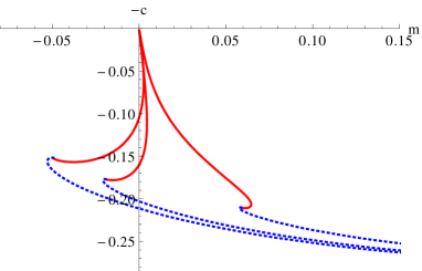
(a) $T=0.24$. $E=0.0001,0.049,0.1$ from left.

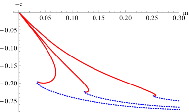
(b) $T=0.30$. $E=0.0001,0.100,0.180$ from left.

Figure 4: $c$-$m$ diagram at finite $E$ parallel to finite $B$ at finite (high) temperature.

The resulting phase diagram is Fig 1(b). For $T\lesssim 0.233$, three regions, as at zero $T$, exist: as $E$ increases, the phases changes from a $\chi$SB insulator (stable meson) phase to a $\chi$SB conductor at a first order transition. There is then a second order transition to a $\chi$S conductor. Above $T\sim 0.233$ the intermediate region $\chi$SB and conductor phase disappears and the chiral symmetry restoration and insulator-conductor transition happen at the same time. It is a first order transition and exists in the temperature range $0.233\lesssim T\lesssim 0.25$. Finally for higher temperatures $T\gtrsim 0.25$, the system becomes a chiral symmetric conductor for any finite $E$.

There are distinct features of the phase diagram though from the $T,\mu$ phase diagram in Fig 1(a). The insulator-conductor transition is first order along its whole length. At finite mass and zero magnetic field, this insulator-conductor transition was also shown to be first order in Veselin1 ; Erdmenger1 . The chiral symmetry restoration phase transition is second order along all its length from the critical point where it joins the insulator-conductor transition. The ability to reproduce different phase structures is interesting and potentially useful if one wanted to use these models as effective descriptions of more complex gauge theories or condensed matter systems.

5 $B$, $\mu$, $E$ at zero temperature

We now turn to the $E,\mu$ plane at fixed B and zero $T$ where the behaviour appears somewhat different from those of the planes so far discussed.

From (17) with $T=0$

$$\widetilde{\mbox{${\cal L}$}}_{LT}=\sqrt{(1+L^{\prime 2})}\sqrt{\left(1-\frac{E^{2}}{w^{4}}\right)\left[\rho^{6}+\frac{\rho^{6}}{w^{4}}+d^{2}-J^{2}\right]}\ ,$$ (25)

and

$$J=\frac{\sqrt{d^{2}w_{s}^{4}+(1+w_{s}^{4})\rho_{s}^{6}}}{w_{s}^{2}}=\sqrt{d^{2}+(1+E^{2})E\cos^{6}\theta_{s}}\ ,$$ (26)

where $w_{s}=\sqrt{E}$. Note that this formula for $J$ is only valid for finite $E$, because the current $J$ is introduced to make a sign change when $\left(1-\frac{E^{2}}{w^{4}}\right)$ changes sign. If $E=0$ we wouldn’t have any reason to introduce $J$.

If we now substitute $J$ back into $\widetilde{\mbox{${\cal L}$}}_{LT}$ then the $d$ dependence explicitly vanishes, as also observed in Erdmenger1 for the zero $B$ case.

$$\widetilde{\mbox{${\cal L}$}}_{LT}=\sqrt{(1+L^{\prime 2})}\sqrt{\left(1-\frac{E^{2}}{w^{4}}\right)\left[\rho^{6}+\frac{\rho^{6}}{w^{4}}-(1+E^{2})E\cos^{6}\theta_{s}\right]}\ .$$

It is the same action as (21), but the physics could still be different because at finite density the boundary condition for the embedding is different from zero density. Furthermore the current (26) looks different from the $d=0$ case (22) through its $d$ dependence (explicitly and implicitly through $\theta_{s}$). However, at zero temperature and finite $E$, it turns out that the density is always zero, which can be shown as follows. From (11) or (20), at zero $T$,

$$A_{t}^{\prime}=d\sqrt{\frac{(w^{4}-E^{2})(1+L^{\prime 2})}{d^{2}w^{4}+\left[-d^{2}-\left(1+\frac{1}{w_{s}^{4}}\right)\rho_{s}^{6}\right]_{E\neq 0}w^{4}+(1+w^{4})\rho^{6}}}\ ,$$ (27)

where $w=\sqrt{L^{2}+\rho^{2}}$ and the square bracket is the current which must be zero at $E=0$. So, for non-zero $E$, the density cancels in the denominator. Let us first consider a fixed non-zero $E$ and the flat embedding and take the limit $\rho\rightarrow 0$.

$$A_{t}^{\prime}\sim\frac{d}{E+1/E}\frac{1}{\rho^{2}}\ .$$ (28)

Thus $\mu\sim d$ $\times$ a $d$-independent integral that diverges near $\rho=0$. There is, therefore, no way to get a finite $\mu$ from a finite $d$. The only available density is exactly zero and if density is zero we shouldn’t use the relation (27). Any constant $A_{t}$ is an available solution so any constant $\mu$ is allowed.

To confirm this analysis, we numerically evaluate density at small temperatures for four sample points, $(E,\mu)=(3,10),(0.3,10),(3,1),(0.3,1)$, in Fig 5. The density indeed vanishes as $T$ goes to zero. Turning on larger chemical potential does not change the tendency: a $10$ times larger chemical potential vanishes $10$ times faster (compare $\mu=10$ and $\mu=1$). Electric field does not affect this much: $E=3$ and $E=0.3$ at $\mu=1$ are indistinguishable in Fig 5. Thus we find that vanishing density at $T=0$ is consistent with the limit $T\rightarrow 0$.

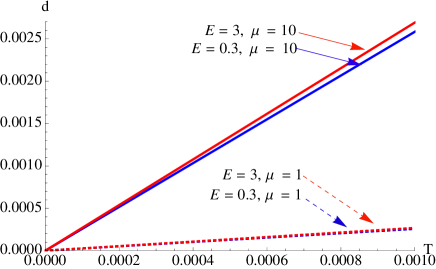
Figure 5: $d$ vs $T$ for four points $(E,\mu)=(3,10),(0.3,10),(3,1),(0.3,1)$. $d\rightarrow 0$ as $T\rightarrow 0$.

Given this argument it is worth checking how nontrivial results come from the same expression on the $\mu$ axis in Fig 1(a), where $T=E=0$. Let us consider $E=0$ not $E\rightarrow 0$.

$$A_{t}^{\prime}=d\sqrt{\frac{w^{4}(1+L^{\prime 2})}{d^{2}w^{4}+(1+w^{4})\rho^{6}}}\ .$$ (29)

For a flat embedding and near $\rho=0$

$$A_{t}^{\prime}\sim 1-\frac{\rho^{2}}{2d^{2}}\ ,$$ (30)

We learn that $\mu\sim d$ $\times$ a $d$-dependent regular integral. So here there is a non-trivial $\mu,d$ relation. We should be careful with the $d\rightarrow 0$ limit. Then the $d$-dependent integral diverges as $d$ gets smaller. However it turns out that it is less divergent than $1/d$ so we get $\mu=0$ as expected. If we consider the spiky embedding then the singular integral will fall as $\sim 1/d$ due to the divergence in $L^{\prime}$. Here we can have a nonzero chemical potential when $d\rightarrow 0$. This occurs at the first transition point (from the solution lying outide the singular shell to the spiky embedding) shown on the $\mu$ axis (zero $T$) in fig 1(a).

Notice that the $T=E=0$ theory and the $T=0$, $E\rightarrow 0$ limit are distinct. The $T=0$, $E,\mu$ plane for any finite $E$ has zero density. However, the strict $E=0$ axis does have density present for the spike and flat embeddings - we show this with the yellow and green lines respectively on the $E=0$ axis in Fig 1(c). Since there is a jump in the density off the $E=0$ axis at $T=0$ there is formally a first order transition with increasing $E$, which is expressed by the blue line near $E=0$ in Fig 1(c). (note the transitions on the $E=0$ axis are second order though - two red dots in Fig 1(c)). In the next section we will approach the $T=0$ plane from positive $T$ to confirm this picture.

The surprising aspect of this result is that, at zero $T$, and with even an infinitessimal $E$ present, density is not generated no matter how large the chemical potential $\mu$ is. Therefore the flat, chirally symmetric configuration is not favoured for very large $\mu$ when a small $E$ is present.

These conclusions are certainly correct within the DBI analysis presented here. If the reader wishes to seek additional physics that might generate density at $T=0,E\neq 0$ and more simply connect the phases at zero and infinitessimal $E$, then one might be able to do that through additional boundary terms at the origin (this is where singular behaviour also enters in the $\mu,d$ relation). Presumably at this point the physics associated with the sink of the energy being injected by the $E$ field should be better understood. Equally the DBI action may not be valid for this system due to a divergent gauge field near the origin KST . Resolving this issue is beyond our DBI analysis here.

6 The Full $B$, $T$, $E$, $\mu$ Phase Structure

Our final task is to complete the phase structure analysis by extending it to the full $E,\mu,T$ volume at fixed $B$. The number of embeddings that must be analyzed on any fixed plane through this space is already large so we restrict ourselves to looking at some representative slices that will be sufficient to reveal the structures present.

In particular we will study fixed $T$ slices and draw the phase structure in the $E,\mu$ plane. The embedding equations are now given by the full forms of (17). To determine the presence and nature of a transition it is sufficient to track any operator of the theory. We have found it easiest on these planes to plot the density $d$ against the chemical potential $\mu$. i.e. we use $d$ as our order parameter.

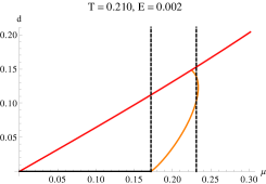
(a) 2nd $\rightarrow$ 1st order

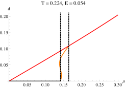
(b) 1st $\rightarrow$ 2nd order

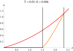
(c) 2nd $\rightarrow$ 2nd order

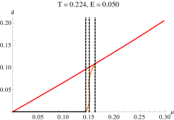
(d) 2nd $\rightarrow$ 1st $\rightarrow$ 2nd order

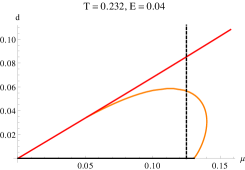
(e) 1st order

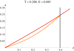
(f) 2nd order

Figure 6: Representative $\mu$-$d$ plots. The black line on the $\mu$ axis corresponds to a embedding that misses the singular shell; the orange curve to a spike embedding that ends on the singular shell; and the red curve to a flat embedding. The transition points are shown by the vertical dotted lines. Subcaptions are the order of transition as $\mu$ increases.

In Fig 6 we show sample plots from which each of a first and second order transition can be identified. There are in total six types of $d$-$\mu$ plots. In each of the figures the black line on the $\mu$ axis corresponds to a chiral symmetry breaking embedding that misses the singular shell; the orange curve to a spike embedding that ends on the singular shell; and the red curve to a flat embedding. It can be seen from the plots whether each transition between embeddings is smooth and hence second order, or whether there is an ‘S’ shaped structure so that one expects a first order transition. The transition points are shown by the vertical dotted lines. We have used these techniques on constant $E$ lines on each constant $T$ plane to determine the transition places and orders. Fig 7 is constructed from sequences of $d$-$\mu$ plots (Fig 6). For example, Fig 7 shows the following evolution of the $d$-$\mu$ plot as $E$ increases.

$$\mathrm{Fig}\ \ref{FixedT} : \qquad\qquad\mathrm{Fig}\ \ref{dmu}$$

$$(a) : \quad(a)\rightarrow(e)\rightarrow(b)\rightarrow(f)$$

$$(b) : \quad(a)\rightarrow(d)\rightarrow(b)\rightarrow(f)$$

$$(c) : \quad(a)\rightarrow(c)\rightarrow(d)\rightarrow(b)\rightarrow(f)$$

$$(d) : \quad(a)\rightarrow(c)\rightarrow(b)\rightarrow(f)$$

$$(e),(f) : \quad(c)\rightarrow(b)\rightarrow(f)$$ (31)

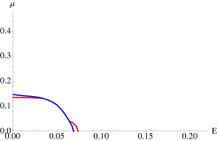
(a) $T=0.232$

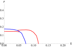
(b) $T=0.224$

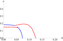
(c) $T=0.222$

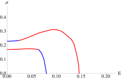
(d) $T=0.210$

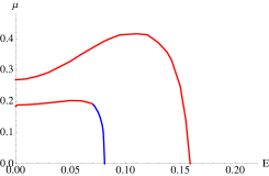
(e) $T=0.200$

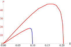
(f) $T=0.003$ (Notice that the scale of $\mu$ is $100$ times larger)

Figure 7: Phase diagrams in the $\mu-E$ plane at various values of temprature showing the phase structure. The solid blue lines are first order transitions, the red lines are second order.

In Fig 7 we show six slices through the volume at varying $T$. Starting at high temperature the theory lives in the chirally symmetric phase with unstable mesons and the material is a conductor. As the temperature falls to $T\simeq 0.25$ the first order transition to the chiral symmetry breaking, stable meson, insulator regime begins to appear in the $\mu$-$E$ plane around $\mu=E=0$. That transition then expands away from the origin and remains briefly first order.

Our plot for $T=0.232$ shows the first interesting structure. Two areas in the plane grow out from the first order line bordered by additional second order transitions. In these areas the theory is in a chiral symmetry breaking but conducting phase. The critical points where the first and second order transitions meet migrate inwards along the first order boundary from each axis as the temperature falls and eventually pass each other as shown for $T=0.224$. At temperatures below that point there are constant $E$ trajectories across which there are three transitions. A second order transition from conductor to insulator, a first order transition between two spike embeddings and finally a second order chiral symmetry restoration transition. An example of the relevant density chemical potential plot for this case is in Fig 6(d).

Our plot for $T=0.222$ shows the next key transition. The first order line between the two spike embeddings breaks making the spike embedding phase continuously connected although there is a remnant of the first order transition ending free at a critical point.

The first order transition near the $E=0$ phase boundary then diminish as temperature is further reduced retreating towards the axes - see the plot for $T=0.21$. It has totally disappeared by $T=0.2$. However the first order transition element on the conductor insulator transition grows from the $E$ axis as temperature decrease.

The final interesting feature begins to appear in the plot at $T=0.21$ where the phase boundaries have begun to deform. They expands out to large $\mu$ very rapidly. Note that the scale of the $\mu$ axis at $T=0.03$ is $100$ times larger than the others. If we drew it on the same scale as the others it would look like Fig 1(c): the $\mu$-independence of the $T=0$ limit is starting to be seen. At zero $T$ (Fig 1(c)) there is a first order transition between the $\mu$ axis and the rest of the $\mu,E$ plane - here we see that that forms as the second order boundaries are pressed onto the $\mu$ axis.

These results have been incorporated into the 3D plot in Fig 1(d) which summarizes the full and rich phase structure.

7 Quark Mass

The analysis above has been purely for zero quark mass. We have not performed an analysis of the introduction of a quark mass, however, we note here that an immediate consequence of introducing a small quark mass is that the second order chiral symmetry restoration transitions (the outer red lines in our figures) become crossovers. We would expect some remnant of the first order segment of this transition to remain associated with a transition at which there is a discontiunuity in the quark condensate even in the infinite mass limit where the theory becomes the massive $\mbox{${\cal N}$}=2$ theory (we observed this in the $E=0$ limit in Evans1 ). The insulator conductor transition remains with quark mass and will again become that of the $\mbox{${\cal N}$}=2$ theory at large mass. At finite mass and temperature but without magnetic field, the insulator-conductor transition was shown to be first order in Veselin1 ; Erdmenger1 .

8 Summary

We have explored the phase structure of the ${\cal N}=2$ gauge theory whose dual is the D3/D7 system. A magnetic field, $B$, tries to induce chiral symmetry breaking. An electric field, $E$, tries to disassociate the mesons of the theory and makes it a conductor. Finite density, $d$, (or chemical potential $\mu$) and temperature, T, each favour melting of the mesons. The competition between these effects lead to a rich phase structure.

In Fig 1(a) we display the $T,\mu$ phase plane for the massless theory at fixed magnetic field. There are three phases - at low $T,\mu$ a chiral symmetry breaking phase with stable mesons; at intermediate values a chiral symmetry breaking phase with unstable mesons; and at large $T,\mu$ a chirally symmetric phase with unstable mesons. The transitions between these are a mix of first and second order transitions linked at two critical points.

In Fig 1(b) we show the $T,E$ phase plane for the massless theory at fixed magnetic field. There are again three phases - at low $T,E$ a chiral symmetry breaking phase with stable mesons which acts as an insulator in the presence of a small electric field; at intermediate values a chiral symmetry breaking phase with unstable mesons which is a conductor and sustains a current in the presence of an electric field; and at high $T,E$ a conducting chirally symmetric phase with unstable mesons. The transitions between these are again a mix of first and second order transitions linked at one critical point.

The $E,\mu$ phase plane has rather different structure (Fig 1(c)). In particular for any finite $E$ the plane is $\mu$ independent and density is zero. At low $E$ we have a chiral symmetry breaking, insulator phase; at intermediate $E$ a chiral symmetry breaking but conducting phase; at large $E$ a conducting and chirally symmetric phase. That the presence of infintessimal electric field does not allow density even with a very large chemical potential and stops the restoration of chiral symmetry is rather surprising. The conclusion is certainly correct within the analysis that we have performed. It is possible though that additional stringy physics should be present near the IR boundary in this limit to explain the sink for the energy the $E$ field is injecting. Such physics could potentially change the phase structure at low $T$.

Finally we have explored the full $E,\mu,T$ volume at fixed $B$ to show how these phases are linked. The phase diagram is summarized in Fig 1(d) with the transition boundaries marked.

The variety of phase structure and transition type in such a simple theory is remarkable. Whether these results can serve as an exemplar for other gauge theories either qualitatively or quantitatively remains to be seen but they certainly suggest a rich structure of phases will be present in many gauge theories.

Acknowledgements: NE is grateful for the support of an STFC rolling grant. KK and AG are grateful for University of Southampton Scholarships. We would like to thank Jonathan Shock, Javier Tarrio, Andy O’Bannon, and Veselin Filev for discussions.

References

- (1) J. M. Maldacena, Adv. Theor. Math. Phys. 2, 231 (1998) Int. J. Theor. Phys. 38, 1113 (1999) [arXiv:hep-th/9711200].
- (2) E. Witten, Adv. Theor. Math. Phys. 2 (1998) 253 [arXiv:hep-th/9802150].
- (3) S. S. Gubser, I. R. Klebanov and A. M. Polyakov, Phys. Lett. B 428 (1998) 105 [arXiv:hep-th/9802109].
- (4) A. Karch and E. Katz, JHEP 0206, 043 (2002) [arXiv:hep-th/0205236].
- (5) M. Grana and J. Polchinski, Phys. Rev. D65 (2002) 126005, [arXiv: hep-th/0106014].
- (6) M. Bertolini, P. Di Vecchia, M. Frau, A. Lerda and R. Marotta, Nucl. Phys. B 621, 157 (2002) [arXiv:hep-th/0107057].
- (7) M. Kruczenski, D. Mateos, R. C. Myers and D. J. Winters, JHEP 0307 049, 2003 [arXiv:hep-th/0304032].
- (8) J. Erdmenger, N. Evans, I. Kirsch and E. Threlfall, Eur. Phys. J. A 35 (2008) 81 [arXiv:0711.4467 [hep-th]].
- (9) V. G. Filev, C. V. Johnson, R. C. Rashkov and K. S. Viswanathan, JHEP 0710, 019 (2007) [arXiv:hep-th/0701001]; T. Albash, V. G. Filev, C. V. Johnson and A. Kundu, JHEP 0807, 080 (2008) [arXiv:0709.1547 [hep-th]]; V. G. Filev, C. V. Johnson and J. P. Shock, JHEP 0908 (2009) 013 [arXiv:0903.5345 [hep-th]].
- (10) N. Evans, A. Gebauer, K. Y. Kim and M. Magou, arXiv:1003.2694 [hep-th].
- (11) K. Jensen, A. Karch, D. T. Son and E. G. Thompson, Phys. Rev. Lett. 105, 041601 (2010) [arXiv:1002.3159 [hep-th]].
- (12) N. Evans, K. Jensen and K. Y. Kim, Phys. Rev. D 82, 105012 (2010) [arXiv:1008.1889 [hep-th]].
- (13) N. Evans, A. Gebauer, K. Y. Kim and M. Magou, JHEP 1003, 132 (2010) [arXiv:1002.1885 [hep-th]].
- (14) J. Babington, J. Erdmenger, N. J. Evans, Z. Guralnik and I. Kirsch, Phys. Rev. D 69 (2004) 066007 [arXiv:hep-th/0306018]; T. Albash, V. G. Filev, C. V. Johnson and A. Kundu, Phys. Rev. D 77 (2008) 066004 [arXiv:hep-th/0605088]; D. Mateos, R. C. Myers and R. M. Thomson, Phys. Rev. Lett. 97 (2006) 091601 [arXiv:hep-th/0605046]; D. Mateos, R. C. Myers and R. M. Thomson, JHEP 0705, 067 (2007) [arXiv:hep-th/0701132].
- (15) S. Nakamura, Y. Seo, S. J. Sin and K. P. Yogendran, J. Korean Phys. Soc. 52, 1734 (2008) [arXiv:hep-th/0611021]; S. Kobayashi, D. Mateos, S. Matsuura, R. C. Myers and R. M. Thomson, JHEP 0702, 016 (2007) [arXiv:hep-th/0611099]; S. Nakamura, Y. Seo, S. J. Sin and K. P. Yogendran, Prog. Theor. Phys. 120, 51 (2008) [arXiv:0708.2818 [hep-th]]; D. Mateos, S. Matsuura, R. C. Myers and R. M. Thomson, JHEP 0711 (2007) 085 [arXiv:0709.1225 [hep-th]].
- (16) J. Grosse, R. A. Janik and P. Surowka, Phys. Rev. D 77 (2008) 066010 [arXiv:0709.3910 [hep-th]].
- (17) N. Evans, T. Kalaydzhyan, K. Y. Kim and I. Kirsch, JHEP 1101, 050 (2011) [arXiv:1011.2519 [hep-th]].
- (18) G. Guralnik, Z. Guralnik and C. Pehlevan, arXiv:1101.3095 [hep-th].
- (19) N. Evans, J. French and K. Y. Kim, JHEP 1011, 145 (2010) [arXiv:1009.5678 [hep-th]].
- (20) A. Karch and A. O’Bannon, JHEP 0709, 024 (2007) [arXiv:0705.3870 [hep-th]].
- (21) A. O’Bannon, Phys. Rev. D 76, 086007 (2007) [arXiv:0708.1994 [hep-th]].
- (22) J. Erdmenger, R. Meyer and J. P. Shock, JHEP 0712, 091 (2007) [arXiv:0709.1551 [hep-th]].
- (23) T. Albash, V. G. Filev, C. V. Johnson and A. Kundu, JHEP 0808, 092 (2008) [arXiv:0709.1554 [hep-th]].
- (24) A. Karch, A. O’Bannon and E. Thompson, JHEP 0904, 021 (2009) [arXiv:0812.3629 [hep-th]].
- (25) J. Mas, J. P. Shock and J. Tarrio, JHEP 0909, 032 (2009) [arXiv:0904.3905 [hep-th]].
- (26) M. Ammon, T. H. Ngo and A. O’Bannon, JHEP 0910, 027 (2009) [arXiv:0908.2625 [hep-th]].
- (27) K. Y. Kim, J. P. Shock and J. Tarrio, arXiv:1103.4581 [hep-th].
- (28) K. Peeters, J. Sonnenschein and M. Zamaklar, Phys. Rev. D 74 (2006) 106008 [arXiv:hep-th/0606195]; C. Hoyos-Badajoz, K. Landsteiner and S. Montero, JHEP 0704 (2007) 031 [arXiv:hep-th/0612169].
- (29) R. Apreda, J. Erdmenger, N. Evans and Z. Guralnik, Phys. Rev. D 71, 126002 (2005) [arXiv:hep-th/0504151].
- (30) K. Y. Kim, S. J. Sin and I. Zahed, arXiv:hep-th/0608046; K. Y. Kim, S. J. Sin and I. Zahed, JHEP 0801, 002 (2008) [arXiv:0708.1469 [hep-th]];
- (31) K. -Y. Kim, S. -J. Sin, I. Zahed, JHEP 0807, 096 (2008). [arXiv:0803.0318 [hep-th]]; A. Davody, [arXiv:1102.4509 [hep-th]].