The Cluster Lensing and Supernova Survey with Hubble (CLASH): Strong Lensing Analysis of Abell 383 from 16-Band HST WFC3/ACS Imaging

Abstract

We examine the inner mass distribution of the relaxed galaxy cluster Abell 383 ($z=0.189$), in deep 16-band HST/ACS+WFC3 imaging taken as part of the CLASH multi-cycle treasury program. Our program is designed to study the dark matter distribution in 25 massive clusters, and balances depth with a wide wavelength coverage, 2000–16000Å, to better identify lensed systems and generate precise photometric redshifts. This photometric information together with the predictive strength of our strong-lensing analysis method identifies 13 new multiply-lensed images and candidates, so that a total of 27 multiple-images of 9 systems are used to tightly constrain the inner mass profile gradient, $d\log\Sigma/d\log r\simeq-0.6\pm 0.1$ ($r<160$kpc). We find consistency with the standard distance-redshift relation for the full range spanned by the lensed images, $1.01<z<6.03$, with the higher redshift sources deflected through larger angles as expected. The inner mass profile derived here is consistent with the results of our independent weak-lensing analysis of wide-field Subaru images, with good agreement in the region of overlap ($\sim 0.7-1$ arcmin). Combining weak and strong lensing, the overall mass profile is well fitted by an NFW profile with $M_{vir}=(5.37^{+0.70}_{-0.63}\pm 0.26)\times 10^{14}M_{\odot}/h$ and a relatively high concentration, $c_{vir}=8.77^{+0.44}_{-0.42}\pm 0.23$, which lies above the standard $c$–$M$ relation similar to other well-studied clusters. The critical radius of Abell 383 is modest by the standards of other lensing clusters, $r_{E}\simeq 16\pm 2\arcsec$ (for $z_{s}=2.55$), so the relatively large number of lensed images uncovered here with precise photometric redshifts validates our imaging strategy for the CLASH survey. In total we aim to provide similarly high-quality lensing data for 25 clusters, 20 of which are X-ray selected relaxed clusters, enabling a precise determination of the representative mass profile free from lensing bias.

1. Introduction

Clusters of galaxies play a direct and fundamental role in testing cosmological models and in constraining the properties of dark matter (DM), providing unique and independent tests of any viable cosmology and structure formation scenario (e.g., Lahav et al., 1991; Evrard et al., 2002; Broadhurst et al., 2005a; Lemze et al., 2009; Jullo et al., 2010). Their extreme virial masses mean that unlike individual galaxies, gas cooling is not capable of compressing the dark matter halo, so that cluster mass profiles reflect directly the thermal evolution of the DM and the growth of the cosmological density field (Peebles, 1985; Duffy et al., 2010). The capability of clusters to critically examine the standard cosmological model is now welcomed more than ever given the unattractive hybrid nature of the standard $\Lambda$CDM model derived by other means.

Simulated CDM dominated halos consistently predict mass profiles that steepen with radius, providing a distinctive, fundamental prediction for this form of DM (Navarro et al. (1996); NFW). Furthermore, the degree of mass concentration should decline with increasing cluster mass because clusters that are more massive, collapse later, when the cosmological background density is lower (e.g., Bullock et al., 2001; Zhao et al., 2003; Neto et al., 2007). Cluster lensing provides a model independent means of testing these fundamental predictions. Given an unbiased sample of relaxed clusters with high spatial resolution, one can rigorously test these basic predictions of the standard $\Lambda$CDM model and contending scenarios. To date, only limited progress has been made toward these aims given the considerable observational challenges of obtaining data of sufficient quality for accurate weak and strong lensing work.

Full mass profiles spanning the weak and strong lensing regimes have been constructed for only a handful of clusters, involving deep HST data to reliably identify large samples of multiple images, and high quality wide-field imaging for careful weak-lensing (WL) work (e.g., Gavazzi et al., 2003; Broadhurst et al., 2005a, 2008; Umetsu & Broadhurst, 2008; Merten et al., 2009, 2011; Newman et al., 2009; Coe et al., 2010; Umetsu et al., 2010, 2011b; Zitrin et al., 2010). It has become clear that the inner mass profile can be accurately obtained using several sets of multiple images spanning a wide range of redshifts (Zitrin et al., 2009b, 2010, 2011c). In the case of WL the data are readily invertible to obtain a model-independent mass profile (Kaiser & Squires, 1993), but much published work has suffered from a significant dilution of the lensing signal by foreground objects and cluster members, leading to shallow profiles with underestimated Einstein radii. The ability of multi-color photometry to isolate foreground and background with reference to the radial WL signal has been demonstrated by Medezinski et al. (2010), so that the WL signal is found to be higher than earlier work, particularly so towards the center of the cluster.

The initial results from combining deep strong-lensing (SL) work with minimally-diluted WL analyses has led to intriguing results, in the sense that although the mass profiles are well fitted by NFW-like profiles, showing the continuously steepening logarithmic gradient consistent with the expected form for CDM dominated halos, the concentration of matter in these halos seems to lie above the mass-concentration relation predicted by the standard $\Lambda$CDM model (Gavazzi et al., 2003; Broadhurst et al., 2005a; Zitrin et al., 2010; Umetsu et al., 2011b). Lensing bias is an issue here for clusters which are primarily selected by their lensing properties, where the major axis of a cluster may be aligned preferentially close to the line of sight, boosting the projected mass density observed (e.g., Hennawi et al., 2007; Corless & King, 2009; Oguri & Blandford, 2009; Sereno et al., 2010; Morandi et al., 2011). This will usually result also in higher measured concentrations and larger Einstein radii (e.g., Sadeh & Rephaeli, 2008; Meneghetti et al., 2010a), though even with these effects taken into account there seems to be some discrepancy from $\Lambda$CDM predictions (Oguri et al., 2009; Meneghetti et al., 2011; Zitrin et al., 2011a). While existing data may not support a strong conclusion that the observations are in significant tension with the standard $\Lambda$CDM model, it is clear that a larger X-ray selected sample, with minimal lensing bias and excellent SL and WL data, is required to evaluate the significance of these trends.

Several examples of high-redshift virialized clusters with diffuse X-ray emission are known, where the highest-redshift cluster selected by X-ray means is now established at $z=2.07$ (CL J1449+0856; Gobat et al. 2011). The most massive of these clusters is XMMU J2235.3-2557 at $z=1.39$ (Rosati et al., 2009) with an estimated total mass of $M_{tot}(<1Mpc)=(5.9\pm 1.3)\times 10^{14}M_{\odot}$. The existence of these clusters, as well as the existence of evolved galaxies at high redshift, are claimed to be unlikely given the predicted abundance of extreme perturbations of cluster sized masses in the standard $\Lambda$CDM scenario (e.g., Daddi et al., 2007, 2009; Collins et al., 2009; Jee et al., 2009; Richard et al., 2011), pointing towards a more extended early history of growth, or a non-Gaussian distribution of massive perturbations.

To shed new light on these mysteries we have embarked on a major project involving galaxy clusters, the Cluster Lensing And Supernova survey with Hubble (CLASH). For more details see Postman et al. (2011). The CLASH program has been awarded 524 orbits of HST time to conduct a multi-cycle program that will couple the gravitational-lensing power of 25 massive intermediate redshift galaxy clusters with HST’s newly enhanced panchromatic imaging capabilities (WFC3 and the restored ACS), in order to test structure formation models with unprecedented precision. The CLASH observations, combined with our wide-field optical and X-ray imaging, represent a substantial advance in the quality and quantity of SL data, enabling us to measure the dark matter mass profile shapes and mass concentrations from hundreds of multiply-imaged sources, providing precise ($\sim 10\%$) observational challenges to scenarios for the DM mass distribution (for full details about the CLASH program see Postman et al. 2011).

The 16 HST bands chosen for this project ranging from the UV through the optical and to the IR, and additional spectra available from large ground-based telescopes for some of the brighter arcs, enable us to obtain accurate redshifts for the multiply-lensed sources presented in this work. We use these remarkable imaging data along with our well-tested approach to SL modeling (e.g., Broadhurst et al., 2005b; Zitrin et al., 2009a, b, 2010, 2011a, 2011c), in order to find a significant number of multiple images across the central field of Abell 383 (A383 hereafter) so that its mass distribution and profile can be constrained with high precision. Various other mass models for this cluster were previously presented (e.g., Smith et al., 2001, 2005; Sand et al., 2004, 2008; Newman et al., 2011) usually based on WFPC2/HST single-band observations, uncovering 3-4 multiple image-systems and various candidates, as will be further discussed in §4.1.

The approach to SL modeling implemented here involves only six free parameters so that in practice the number of multiple images uncovered readily exceeds the number of free parameters as minimally required in order to obtain a reliable fit, allowing for identification of other multiply-lensed systems across the cluster field. Our approach to lens-modeling is based on the reasonable assumption that mass approximately traces light. We have independently tested this assumption in Abell 1703 (Zitrin et al., 2010), by applying the non-parametric technique of Liesenborgs et al. (2006, 2007, 2009) for comparison, yielding similar results. Such parameter-free methods usually do not have the precision to actually find new multiple-images, but the resulting 1D radial profiles are sufficiently accurate for meaningful comparisons. Independently, it has been found that SL methods based on parametric modeling are accurate at the level of a few percent in determining the projected inner mass (Meneghetti et al., 2010b).

The paper is organized as follows: In §2 we describe the observations, and in §3 we detail the SL analysis. In §4 we report and discuss the results where in §5 we compare these to numerical simulations. The results are then summarized in §6. Throughout this paper we adopt a concordance $\Lambda$CDM cosmology with ($\Omega_{\rm m0}=0.3$, $\Omega_{\Lambda 0}=0.7$, $h=0.7$). With these parameters one arcsecond corresponds to a physical scale of 3.17 kpc for this cluster (at $z=0.189$; Sand et al. 2004). The reference center of our analysis is fixed on the brightest cluster galaxy (BCG): RA = 02:48:03.41 Dec = -03:31:44.91 (J2000.0).

2. Observations and Redshifts

As part of the CLASH program (see §1), Abell 383 was observed with HST between 2010 November to 2011 March. This is our first of 25 clusters to be observed to a depth of 20 HST orbits in 16 filters with the Wide Field Camera 3 (WFC3) UVIS and IR cameras, and the Advanced Camera for Surveys (ACS) WFC. Observation details and filters are provided in Table 1.

The images are processed for debias, flats, superflats, and darks, using standard techniques. The ACS images are further corrected for bias striping (Grogin et al., 2010) and CTE/CTI degradation effects (Anderson & Bedin, 2010). WFC3/IR pixels are flagged and downweighted for persistence effects. All images are then co-aligned and combined using drizzle algorithms to a scale of $0.065\arcsec/$ pixel. An additional set of images with the original ACS $0.05\arcsec/$ pixel scale is produced, onto which we apply our modeling initially to maintain the higher resolution, where the full UVIS/ACS/WFC3-IR data set is then importantly used for multiple-images verification and measurement of their photometric redshifts. Further details of our pipeline will be presented in an upcoming paper.

Based on the 16-filter photometry, we obtain photometric redshifts using BPZ (Benítez, 2000; Benítez et al., 2004; Coe et al., 2006) and LePhare (LPZ hereafter; Arnouts et al. 1999; Ilbert et al. 2006). These two methods yielded some of the best results of all photo-z methods tested by the PHoto-z Accuracy Testing group (Hildebrandt et al., 2010). BPZ and LPZ are similar in that spectral energy distribution (SED) templates are redshifted and fit to observed photometry. BPZ currently uses 6 templates from PEGASE (Fioc & Rocca-Volmerange, 1997), calibrated using the FIREWORKS photometry and spectroscopic redshifts from Wuyts et al. (2008). LPZ uses templates from Bruzual & Charlot (2003) calibrated using COSMOS (Koekemoer et al., 2007) photometry and spectroscopic redshifts as described in Ilbert et al. (2009). The templates are empirically generated, describing well the full range of galaxy colors found in these multiband catalogs (less than $\sim 1\%$ outliers for high quality spectroscopic samples), and therefore implicitly encompass all the range of metallicities, extinctions, and star formation histories of real galaxies. Further details on these methods can be found in the aforementioned references. While similar, the two methods serve as important cross-checks of one another.

The distances to the galaxies are, of course, key ingredients to the lens model. The photo-z analyses used here also clearly aid us in assessing the robustness of the multiple-image identifications. The photometry of some lensed images may be significantly contaminated by brighter nearby cluster galaxies. SExtractor attempts to correct for this by measuring and subtracting the local background around each object. This works well in some cases but not all. To better reveal these lensed galaxies, we have carefully modeled and subtracted the light of several cluster galaxies including the BCG. While this improved the detection of some lensed galaxies, it did not consistently improve their photometry and thus photometric redshifts. The cluster galaxy wings must be modeled and subtracted very robustly and consistently to achieve quality photometry in all 16 bands for faint, nearby galaxy images.

Explicitly, for its subtraction, the BCG has been modeled using the CHEF basis (Jiménez-Teja & Benítez, 2011). This basis comprises both Chebyshev rational and trigonometric functions, ensuring that the extended disk of this object is properly modeled. The flexibility of the CHEFs scale parameter allows us to accurately represent the BCG while keeping significant substructure and arcs unchanged. An example of the BCG subtraction is seen in Figure 2.

Our 16 filters were selected based on tests with simulated photometry to yield precise ($\Delta z\sim 0.02(1+z)$) photo-z’s (Postman et al., 2011). Previous work has also demonstrated how photo-z precision improves by increasing the number of (preferably overlapping) filters for a fixed total observing time (Benítez et al., 2009b). The empirical precision of CLASH photo-z’s for arcs and other galaxies, including the relative contributions of various filters, will be detailed in future work.

Table 1CLASH HST Observation Log for A383

Filter	Assigned orbits	Total time (s)	Instrument
F225W	1.5	3672	WFC3/UVIS
F275W	1.5	3672	WFC3/UVIS
F336W	1.0	2434	WFC3/UVIS
F390W	1.0	2434	WFC3/UVIS
F435W	1.0	2125	ACS/WFC
F475W	1.0	2064	ACS/WFC
F606W	1.0	2105	ACS/WFC
F625W	1.0	2064	ACS/WFC
F775W	1.0	2042	ACS/WFC
F814W	2.0	4243	ACS/WFC
F850LP	2.0	4214	ACS/WFC
F105W	1.1	2815	WFC3/IR
F110W	1.0	2515	WFC3/IR
F125W	1.0	2515	WFC3/IR
F140W	1.0	2412	WFC3/IR
F160W	2.0	5029	WFC3/IR

3. Strong Lensing Modeling and Analysis

We apply our well tested approach to lens modeling, which has previously uncovered large numbers of multiply-lensed galaxies in ACS images of Abell 1689, Cl0024, 12 high-$z$ MACS clusters, MS 1358, and the “Pandora cluster” Abell 2744 (respectively, Broadhurst et al., 2005b; Zitrin et al., 2009b, 2011a, 2011c; Merten et al., 2011). Briefly, the basic assumption adopted is that mass approximately traces light, so that the photometry of the red cluster member galaxies is used as the starting point for our model. Cluster member galaxies are identified as lying close to the cluster sequence by the photometry described in §2. In addition, using our extensive 16-band imaging and corresponding photometric redshifts, these can be then verified as members lying at the cluster’s redshift.

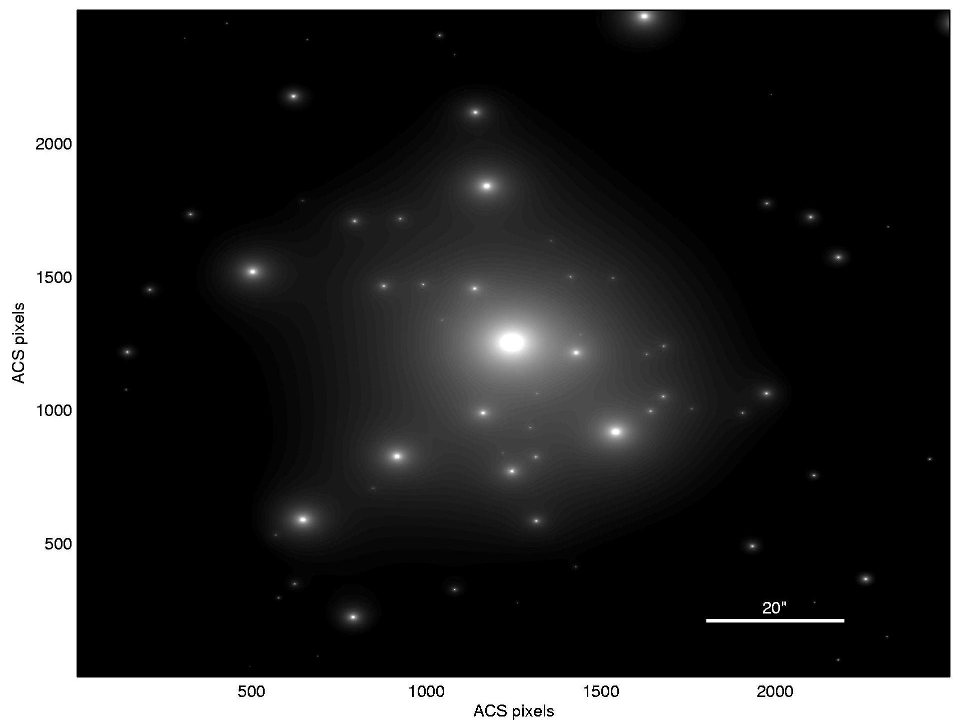
Figure 1.— The starting point of the mass model, where we define the surface mass distribution based on the cluster member galaxies (see §3). Axes are in ACS pixels ($0.05\arcsec/pixel$), and a $20\arcsec$ bar is overplotted. North is up, East is left.

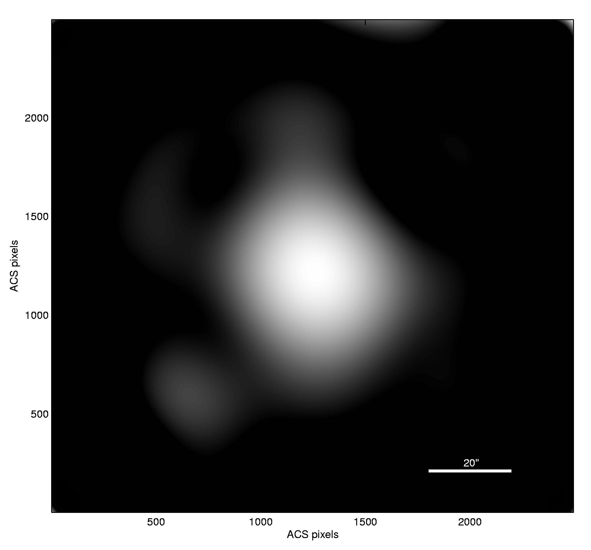
Figure 2.— The resulting smooth mass component of the mass model (see §3). Axes are in ACS pixels ($0.05\arcsec/pixel$), and a $20\arcsec$ bar is overplotted. North is up, East is left.

We approximate the large scale distribution of cluster mass by assigning a power-law mass profile to each galaxy (see Figure 1), the sum of which is then smoothed (see Figure 2). The degree of smoothing ($S$) and the index of the power-law ($q$) are the most important free parameters determining the mass profile. A worthwhile improvement in fitting the location of the lensed images is generally found by expanding to first order the gravitational potential of this smooth component, equivalent to a coherent shear describing the overall matter ellipticity. The direction of the shear ($\phi_{\gamma}$) and its amplitude ($|\gamma|$) are free parameters, allowing for some flexibility in the relation between the distribution of DM and the distribution of galaxies, which cannot be expected to trace each other in detail. The total deflection field $\vec{\alpha}_{T}(\vec{\theta})$, consists of the galaxy component, $\vec{\alpha}_{gal}(\vec{\theta})$, scaled by a factor $K_{gal}$, the cluster DM component $\vec{\alpha}_{DM}(\vec{\theta})$, scaled by (1-$K_{gal}$), and the external shear component $\vec{\alpha}_{ex}(\vec{\theta})$, all scaled by the overall normalization factor $K_{q}$:

$$\vec{\alpha}_{T}(\vec{\theta})=K_{q}(K_{gal}\vec{\alpha}_{gal}(\vec{\theta})+(1-K_{gal})\vec{\alpha}_{DM}(\vec{\theta})+\vec{\alpha}_{ex}(\vec{\theta})),$$ (1)

where the deflection field at position $\vec{\theta}_{m}$ due to the external shear, $\vec{\alpha}_{ex}(\vec{\theta}_{m})=(\alpha_{ex,x},\alpha_{ex,y})$, is given by:

$$\alpha_{ex,x}(\vec{\theta}_{m})=|\gamma|\cos(2\phi_{\gamma})\Delta x_{m}+|\gamma|\sin(2\phi_{\gamma})\Delta y_{m},$$ (2)

$$\alpha_{ex,y}(\vec{\theta}_{m})=|\gamma|\sin(2\phi_{\gamma})\Delta x_{m}-|\gamma|\cos(2\phi_{\gamma})\Delta y_{m},$$ (3)

where $(\Delta x_{m},\Delta y_{m})$ is the displacement vector of the position $\vec{\theta}_{m}$ with respect to a fiducial reference position, which we take as the lower-left pixel position $(1,1)$, and $\phi_{\gamma}$ is the position angle of the spin-2 external gravitational shear, measured counter-clockwise from the $x$-axis. The normalization of the model ($K_{q}$) and the relative scaling of the smooth DM component versus the galaxy contribution ($K_{gal}$) bring the total number of free parameters in the model to 6 (see Zitrin et al. 2009b for more details). This approach to SL is sufficient to accurately predict the locations and internal structure of multiple images, since in practice the number of multiple images uncovered readily exceeds the number of free parameters, so that the fit is fully constrained.

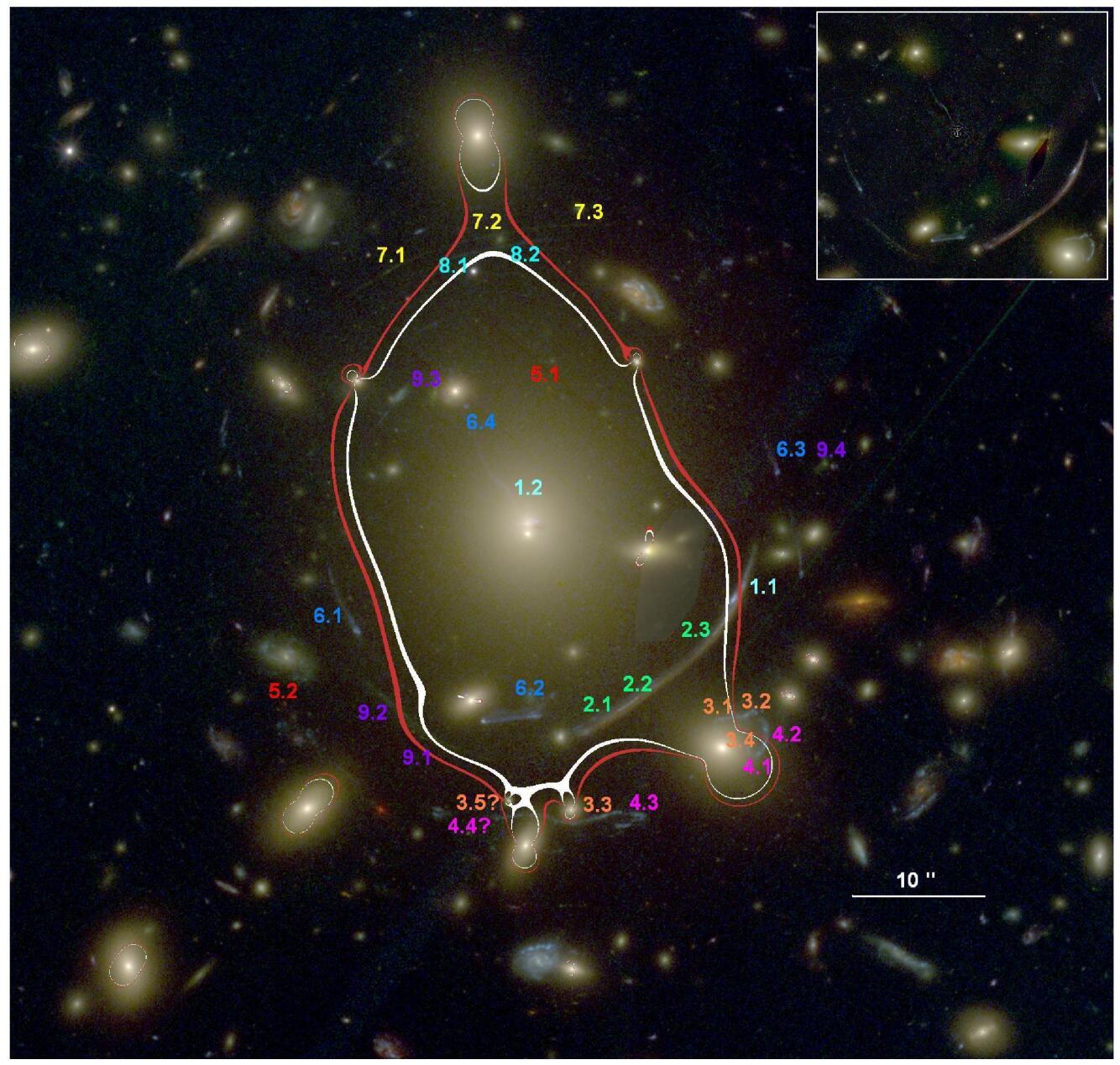
Figure 3.— Galaxy cluster A383 ($z=0.189$) imaged with HST/ACS/WFC3. North is up, East is left. We number the multiply-lensed images used and uncovered in this work. The numbers indicate the 27 lensed images, 13 of which correspond to 4 newly identified sources, and the different colors are used to distinguish the 9 different sources. For more details on the each system and the robustness of the new identifications see §4.1. The overlaid white critical curve corresponds to systems 3 and 4, at $z_{s}=2.55$, enclosing a critical area of an effective Einstein radius of $\simeq 52$ kpc at the redshift of this cluster ($16.3\arcsec$). Also plotted is a red critical curve, which corresponds to system 5, the drop-out high redshift galaxy at $z_{s}=6.027$. The composition of this color image is Red=F105W+F110W+F125W+F140W+F160W, Green=F606W+F625W+F775W+F814W+F850LP, and Blue=F435W+F475W. This image was generated automatically by using the freely available Trilogy software. The upper-right inset shows the central core with the BCG subtracted, using the method of Jiménez-Teja & Benítez (2011, see also §2).

In addition, two of the six free parameters, namely the galaxy power law index $q$, and the smoothing degree $S$, can be primarily set to reasonable values so that only 4 of the free parameters have to be constrained initially, which sets a very reliable starting-point using obvious or known systems. This is because these two parameters control the mass slope, but the overall mass distribution and corresponding critical curves do not strongly depend on them. The mass distribution is therefore primarily well constrained, uncovering many multiple-images which can then be iteratively incorporated into the model, by using their redshift estimation and location in the image-plane.

We use this preliminary model to delens the more obvious lensed galaxies back to the source plane by subtracting the derived deflection field. We then relens the source plane in order to predict the detailed appearance and location of additional counter images, which may then be identified in the data by morphology, internal structure and color. The best fit is assessed by the minimum $\chi^{2}$ uncertainty in the image plane:

$$\chi^{2}=\sum_{i}((x_{i}^{{}^{\prime}}-x_{i})^{2}+(y_{i}^{{}^{\prime}}-y_{i})^{2})~{}/~{}\sigma^{2},$$ (4)

where $x_{i}^{{}^{\prime}}$ and $y_{i}^{{}^{\prime}}$ are the locations given by the model, $x_{i}$ and $y_{i}$ are the real image locations, $\sigma$ is the error in the location measurement (taken as $0.5\arcsec$), and the sum is over all $N$ images. The model location of each image is the averaged location given by relensing all other images of the same system. The best-fit solution is unique in this context, and the model uncertainty is determined by the location (of predicted images) in the image-plane itself. Importantly, this image-plane minimization does not suffer from the bias involved with source-plane minimization, where solutions are biased by minimal scatter towards shallow mass profiles with correspondingly higher magnification.

The model is successively refined as additional sets of multiple images are incorporated to improve the fit, importantly using also their redshift information for better constraining the mass slope. The mass profile is coupled to the redshift distribution of the different systems, since for each redshift the enclosed mass and correspondingly the deflection angle, depend on the lens and source angular-diameter distances ($D_{l}$, $D_{s}$, respectively). Explicitly, the deflection angle is defined as $\alpha(\theta)=\frac{4GM(<\theta)}{c^{2}\theta}\frac{d_{ls}}{d_{s}d_{l}}$, and since the lens distance is constant, the mass slope is constrained through the cosmological relation of the $D_{ls}/D_{s}$ growth with source redshift, where $D_{ls}$ is the distance between the lens and the source. This is seen more clearly in Figure 12.

4. Results and Discussion

4.1. Multiple-Images, Mass Model and Critical Curves

Table 2Multiple-image systems

ARC	RA	DEC	BPZ $z_{phot}$	LPZ $z_{phot}$	spec-$z$	$z_{model}$	Comment
ID	(J2000.0)	(J2000.0)	(best) [95% C.L.]	(best) [99% C.L.]
1.1	02:48:02.331	-03:31:49.72	0.97 [0.83–1.05]	0.93 [0.92–0.93]	1.01	(1.01)
1.2	02:48:03.525	-03:31:41.85	0.53 [0.34–0.59]	0.47 [0.47–0.48]	1.01	”	radial image in BCG halo
2.1	02:48:02.947	-03:31:58.95	0.95 [0.87–1.03]	0.90 [0.90–0.92]	1.01	(1.01)
2.2	02:48:02.852	-03:31:58.04	0.96 [0.82–1.04]	0.85 [0.78–0.93]	1.01	”
2.3	02:48:02.452	-03:31:52.84	0.84 [0.77–0.91]	0.76 [0.67–0.84]	(1.01)	”
3.1	02:48:02.426	-03:31:59.40	2.79 [2.64–2.94]	2.90 [2.54–3.15]	2.55	(2.55)
3.2	02:48:02.309	-03:31:59.21	2.90 [2.75–3.05]	3.01 [2.92–3.08]	2.55	”
3.3	02:48:03.026	-03:32:06.75	2.56 [2.42–2.70]	3.03 [2.86–3.09]	2.55	”
3.4	02:48:02.300	-03:32:01.74	2.88 [2.73–3.05]	3.01 [2.87–3.16]	(2.55)	”
4.1	02:48:02.244	-03:32:02.07	0.20 [0.15–0.25]	0.20 [0.20–0.26]	2.55	(2.55)
4.2	02:48:02.214	-03:32:00.25	2.85 [2.70–3.00]	2.91 [2.82–3.01]	2.55	”
4.3	02:48:02.847	-03:32:06.68	3.09 [2.93–3.25]	3.05 [2.91–3.20]	2.55	”
5.1	02:48:03.264	-03:31:34.77	5.95 [5.68–6.22]	5.87 [5.64–5.99]	6.027	(6.027)
5.2	02:48:04.600	-03:31:58.47	6.01 [5.74–6.29]	5.96 [5.72–6.12]	6.027	”
6.1	02:48:04.272	-03:31:52.77	2.67 [2.53–2.81]	2.13 [2.05–2.18]	–	$\simeq 2.0$
6.2	02:48:03.377	-03:31:59.27	2.38 [2.25–2.51]	1.93 [1.90–2.09]	–	”
6.3	02:48:02.153	-03:31:40.88	1.89 [1.78–2.04]	2.10 [1.90–2.20]	–	”
6.4	02:48:03.720	-03:31:35.87	1.80 [1.69–1.91]	1.54 [1.46–1.57]	–	”	bright galaxy nearby
7.1	02:48:04.089	-03:31:25.54	4.60 [0.64–4.82]	4.50 [4.24–4.76]	–	$\simeq 4.6$	bimodal
7.2	02:48:03.568	-03:31:22.55	4.65 [0.38–5.20]	4.77 [0.52–5.58]	–	”	”
7.3	02:48:03.130	-03:31:22.16	4.70 [4.35–5.07]	4.56 [0.20–5.08]	–	”	”
8.1	02:48:03.681	-03:31:24.43	0.34 [0.24–2.43]	0.33 [0.20–3.19]	–	$\simeq 3.1$	bimodal
8.2	02:48:03.386	-03:31:23.46	2.94 [2.41–3.25]	2.93 [0.20–3.46]	–	”
9.1	02:48:03.920	-03:32:00.83	3.91 [3.63–4.10]	3.83 [3.51–4.09]	–	$\simeq 4.0$
9.2	02:48:04.046	-03:31:59.21	0.48 [0.26–0.54]	0.47 [0.39–0.53]	–	”	segment yields $z_{phot}\sim 3.9$, see §4.1
9.3	02:48:03.872	-03:31:35.03	3.96 [3.77–4.15]	3.57 [3.56–3.59]	–	”
9.4	02:48:01.918	-03:31:40.23	3.80 [3.61–3.99]	3.75 [3.57–3.82]	–	”

In addition to the previously-known systems (see Newman et al. 2011 and references therein, Richard et al. 2011), our modeling technique has uncovered 13 new multiply-lensed images and candidates in the central field of A383, belonging to 4 new systems. We thus substantially increase in this work the number of available constraints on the mass profile of this cluster.

We have made use of the location and redshift information of the multiple-images to fully constrain the mass model. In our minimization procedure, we obtain for most important parameters controlling the mass distribution, values of $q=1.08\pm 0.08$ and $S=12\pm 2$, but note these are highly coupled to the photometry used to construct the mass model, and to our procedure detailed in §3.

We find that the critical curve for a source at $z_{s}=2.55$ (systems 3-4) encloses an area with an effective Einstein radius of $r_{E}=16.3\pm 2\arcsec$, or $\simeq$52 kpc at the redshift of the cluster. A projected mass of $M=2.4\pm 0.2\times 10^{13}M_{\odot}$ is enclosed by this critical curve (see Figure 2). For general comparison, this is in good agreement with the Einstein radius-mass relation for a source at $z_{s}\simeq 2-2.5$, found in Zitrin et al. 2011a (taking into account also the different lens distances; see Figure 27 therein). This is naturally expected from the lensing equations, though constitutes an important consistency check. The corresponding critical curves are plotted on the cluster image in Figure 2 along with the multiply-lensed systems. The resulting mass distribution and its profile are shown in Figures 4 and 5.

It should be stressed that the multiple-images found here are accurately reproduced by our model and are not simple identifications by eye. The parametric method of Zitrin et al. (2009b) has been shown in many cases to have the predictive power to find multiple images in clusters. Due to the small number of parameters this model is initially well-constrained enabling a reliable identification of other multiple-images in the field, which can be then used to fine-tune the mass model. Naturally, the mass model predictions have to be identified in the data and verified further by comparing the SEDs and photometric redshifts of the candidate multiple-images, especially in cases where the images are not prominently bright and big, so that internal details cannot be reliably distinguished. As some of the objects identified here are faint and some may be contaminated by nearby cluster members even after their subtraction, for the less secure cases we supply also the photo-$z$ distributions and spectral energy distributions (SEDs) from our 16 HST-band imaging, so that the reader could assess the plausibility of these identifications. We now detail each multiply-lensed system, as listed in Table 2:

$Systems~{}1-2:$ The prominent giant arc, nearly $20\arcsec$ long, most likely consists of two sources (systems 1 and 2 here) at the same redshift of $z_{s}=1.01$ (Sand et al., 2004, 2008; Smith et al., 2005). An additional radial counter image is seen in the BCG halo (see also Newman et al. 2011). This system was identified by Smith et al. (2001) in WFPC2 1-band imaging, who also spectroscopically measured the west side of the arc to be at $z_{s}=1.01$. Following measurement of Sand et al. (2004) with a slit passing through the BCG, the radial arc, and the eastern part of the main arc, yielded an identical redshift of $z_{s}=1.01$ for both as well.

Following examples from other well known clusters, it is not common for a giant arc to consist of two different sources. We therefore primarily do not use the location of the multiple-images of these systems in our minimization (only their redshift), though our model agrees with this previous interpretation and accurately produces these multiple-images at this redshift. In addition, our model suggests that part of the radial arc is also contributed by the left side of the giant arc (system 2). However, it is still plausible that the giant arc consists of only one elongated source. We find that the full giant arc, when projected back to the source plane, corresponds to $\simeq$11 kpc in length, which may indeed be accounted for by a single source. The reproduction of the source is seen in Figure 6.

$Systems~{}3-4:$ Corresponding to a pair of sources, the images of which are lensed to appear next to each other on the two sides of a prominent cluster galaxy, as can be seen in Figure 2. These images were identified by Smith et al. (2001) who mapped the internal structures in detail, and were spectroscopically measured by Newman et al. (2011) to be at a redshift of $z_{s}=2.55$. In addition, our IR/WFC3 images show clearly, for the first time, that these two systems indeed have two different colors and SEDs, and our mass model accurately reproduces each as shown in Figure 7. We note that our model suggests that a small part of the radial arc may consist of a counter image of these systems, in addition to the radial images of systems 1 and 2.

Eastwards to image 3.3 there is a faint arc which might be related either to this system or to system 4. This faint extending arc was marked as part of this system by Smith et al. (2001) but omitted in recent analysis (Newman et al., 2011). We find that this faint arc, marked as 3.5/4.4 here, may be related to this system (also yielding a similar photometric redshift of $\sim 2.7$), and is reproduced as part of this system by our model if we slightly increase the weight of its neighboring galaxy (RA=02:48:03.42, DEC=-03:32:09.02), see Figure 2. On the other hand, the IR colors do not strongly support connection to systems 3 and 4, and this faint arc might be a locally multiply-lensed separate system. In any case its inclusion has only a negligible and local effect on the mass model.

$System~{}5:$ Two images of a multiply-lensed Lyman-break, high redshift galaxy at $z_{s}=6.027$, reported recently by Richard et al. (2011) based on CLASH imaging and Keck spectra. We also identify these two images and measure photometric redshifts of $z\approx 6.01$ and $5.95$. The high redshift of this system expands substantially the lensing-distance range thus enabling us to constrain the profile with better accuracy, as discussed in §4.2.

$System~{}6:$ This system consists of 4 blue images with similar internal details including a brighter white blob, at a typical photometric redshift of $z_{s}\sim 2.4$ for this system (see Table 2, Figure 9). Our model reproduces these images very well (Figure 8), though it slightly favors a lower redshift of $z_{s}\simeq 2$ but due to the distances involved this is in practice only a $\simeq 1\%$ difference in the redshift distance ratio. These images were matched up for the first time in this work enabled by the deep, high-resolution HST data. Due to the variance in the SEDs and therefore photometric redshifts of the images of this system, we supply also the photo-$z$ distributions and SEDs in Figure 9, so that the reader could more easily assess the plausibility of this system.

$Systems~{}7-8:$ Two thin and long arcs following similar symmetry, at a relatively high redshift of $z\sim 4.5$ and $z\sim 3$, respectively. Their symmetry especially with regards to the critical curves, shows beyond a doubt that these are multiply-lensed systems (see also Figure 10), despite being too faint to measure their photometric redshift unambiguously. These images as well were matched up for the first time in this work.

$System~{}9:$ A faint, wide greenish-looking arc $17\arcsec$ south east of the BCG (see Figure 2). Our model accurately reproduces this arc as a double image. In addition, two other small counter-images are predicted, for which we identify the best-matching candidates in the data. These images were matched up for the first time in this work, and except for image 9.2, show similar photometric redshifts of $\sim 3.8$ (see also Figure 11), in agreement with our model prediction. In addition, it should be noted that photo-$z$ analyses of some segments of the arc designated as 9.2 imply indeed a redshift of $\sim 3.8$, similar to the other three images of this system. We also acknowledge the possibility that other similar looking objects near-by images 9.3 and 9.4 may be the actual counter images - especially since 9.3 and 9.4 seem slightly brighter than 9.1 and 9.2. Such a degeneracy however does not affect the mass model in a noticeable way. Due to the variance in the SEDs and therefore photometric redshifts of these images, we supply also their photo-$z$ distributions and SEDs in Figure 11, so that the reader could more easily assess the plausibility of this system.

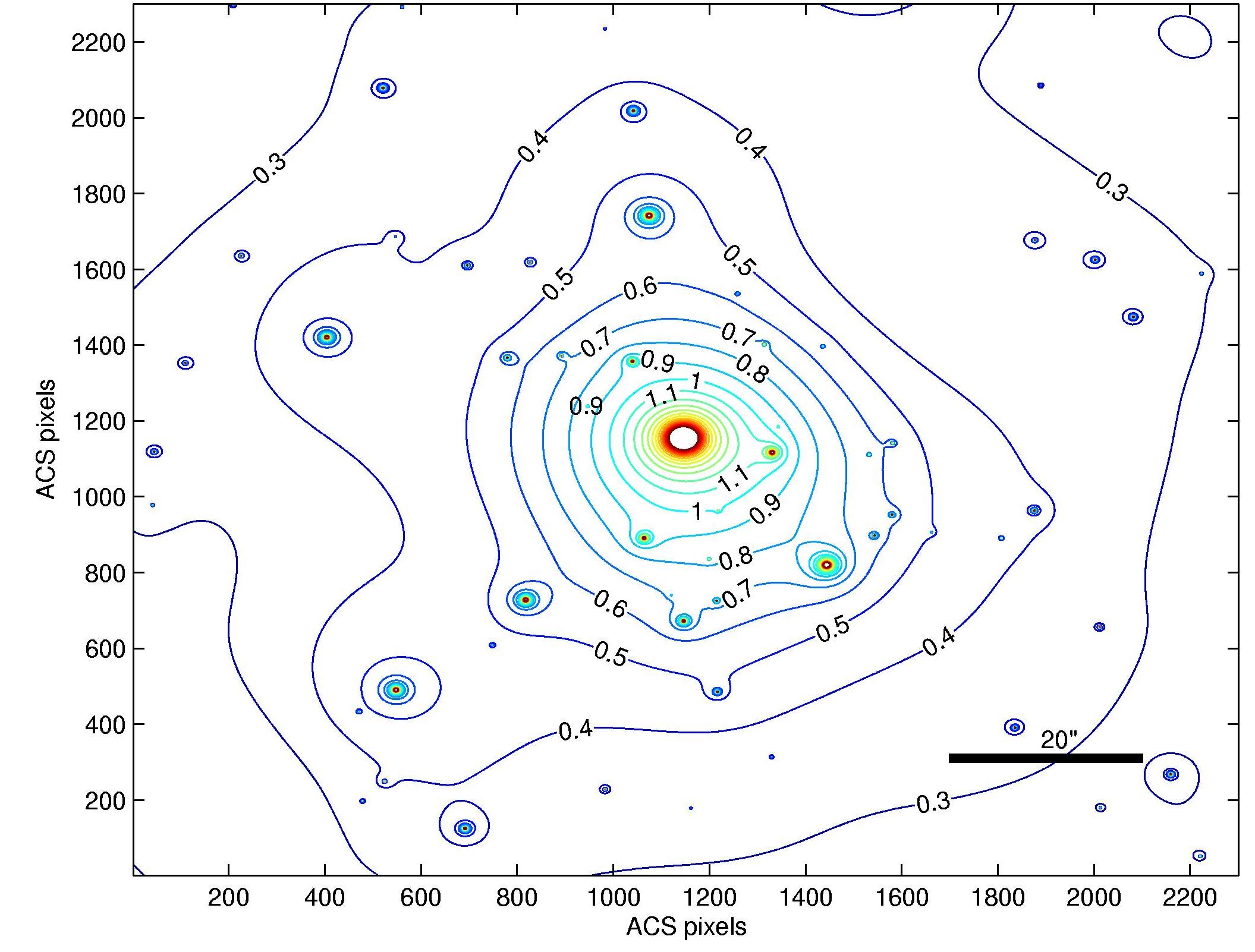
Figure 4.— 2D surface mass distribution ($\kappa$), in units of the critical density (for $z_{s}=2.55$), of A383. Contours are shown in linear units and in spaces of $\Delta\kappa=0.1$, derived from our mass model constrained using the many sets of multiply-lensed images seen in Figure 2. As can be seen, the mass distribution is fairly round. Axes are in ACS pixels ($0.05\arcsec/pixel$), and a $20\arcsec$ bar is overplotted. North is up, East is left.

Figure 5.— Radial surface mass density ($\kappa$) profile in units of the critical surface density (for a source redshift of $z_{s}=2.55$). The inner SL data were derived using the sets of multiple images shown in Figure 2. We overplot our preliminary WL data analysis. As can be seen, these are in very good agreement in the region of overlap. A joint SL+WL gNFW fit yields $M_{vir}=(5.94^{+1.05}_{-0.87}\pm 0.71)\times 10^{14}M_{\odot}/h$ (or $M_{vir}\simeq 8.49\times 10^{14}M_{\odot}$) and a concentration parameter of $c_{-2}=7.95^{+0.89}_{-0.90}\pm 0.55$. The parameter $\alpha=1.078^{+0.069}_{-0.073}\pm 0.059$, so that the overall fit is similar to a simple NFW (see §4.2 for explicit comparison). These values are in common with more massive well studied clusters, and lie above the standard $c$–$M$ relation, as seen in Fig. 13. Also plotted is the 1D WL analysis of Huang et al. (2011). A clear consistency is seen through the extensive WL range, though our profile is more consistent with the SL data and is not underestimated in the inner region. A more thorough, 2D WL analysis will be published soon (Umetsu et al., in preparation).

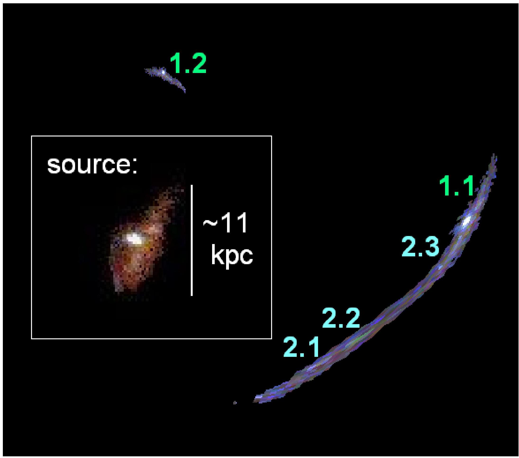
Figure 6.— Reproduction of systems 1 and 2 (consisting the giant arc) by our model. We lens the full giant arc to the source plane and back, with a lensing distance corresponding to $z_{s}=1.01$. Overplotted are the reproduced radial arc, 1.2, and an enlarged image of the reproduced source along with its physical scale. The prominent bright blob lensed in the procedure may be unrelated. The source image had color manipulation and noise cleaning procedures acted on, to better show the internal details.

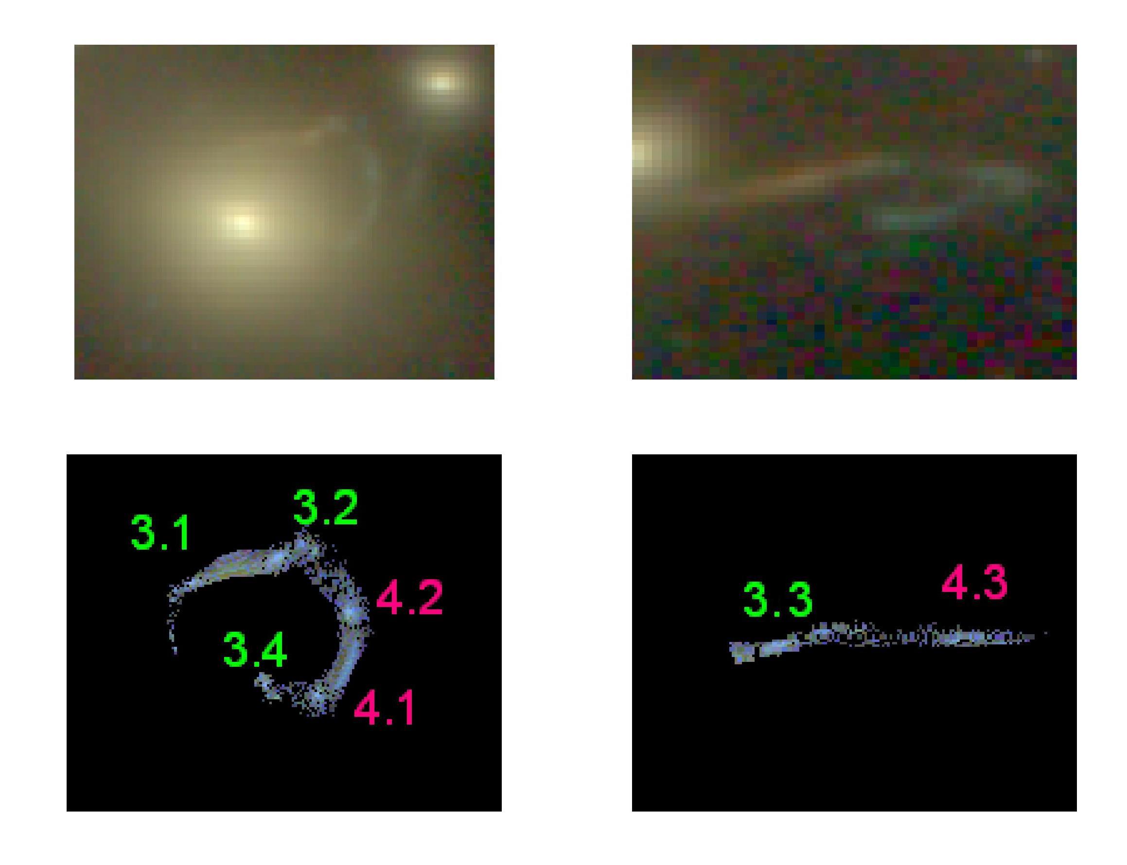
Figure 7.— Reproduction of systems 3 and 4 by our model, by delensing jointly images 3.1 and 4.1 into the source plane with a lensing distance corresponding to $z_{s}=2.55$, and then relensing the resulting source plane pixels onto the image plane. Note the different colors of these systems, seen in an WFC3/IR color image.

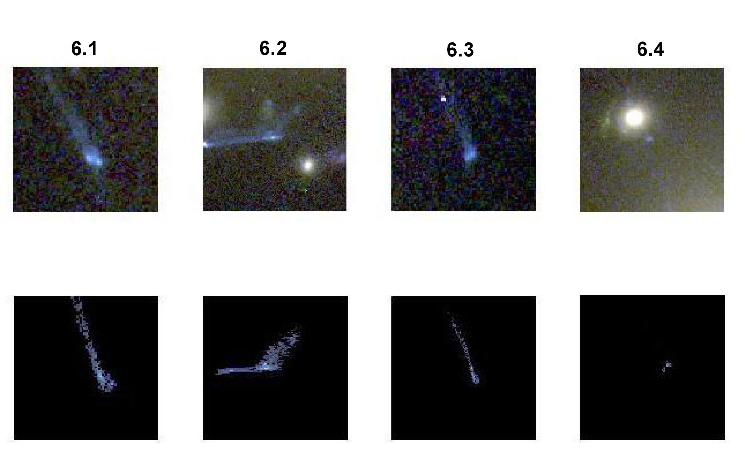
Figure 8.— Reproduction of system 6 by our model, by delensing image 6.2 into the source plane with a lensing distance corresponding to $z_{s}\simeq 2$, and then relensing the resulting source plane pixels onto the image plane. Our model clearly reproduces accurately the other images in this system.

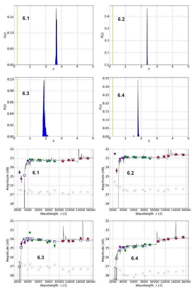
Figure 9.— Photo-$z$ distribution (blue) and 16 HST-band SEDs of the four images of system 6 (see Figure 8), generated using BPZ (§2). As can be seen, the photo-$z$’s support in general our identification of this system, though with some uncertainty and corresponding variation in the SEDs. The yellow stripe in the photo-$z$ distributions corresponds to the cluster redshift at $z=0.189$, and the red crosses in the SED plots mark the $1\sigma$ magnitude detection limit in each filter.

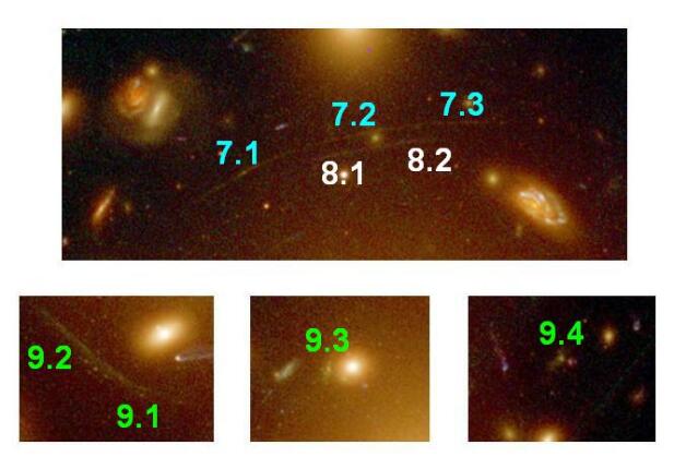
Figure 10.— Stamp images of some of our newly identified multiple-images, seen more clearly in this color-composite image constructed from 16 HST bands ranging from the UV to the IR. As can be seen, systems 7 and 8 follow the same symmetry and are clearly multiple images as supported also by our mass model and photo-$z$’s (see Table 2). In system 9, images 9.1 and 9.2 are clearly multiply-lensed to form the greenish-looking arc, while 9.3 and 9.4 are the most likely counter images as predicted by our model and coherent photo-$z$’s seen in Figure 11. Other similar looking objects are seen close to these images which might be the actual counter images, but such a degeneracy does not affect the mass model in a noticeable way.

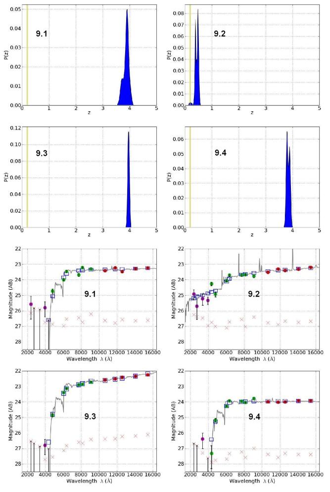
Figure 11.— Another example of the photo-$z$ distribution (blue) and 16 HST-band SEDs, generated using BPZ (§2) and used to match the four images of system 9 (see Figure 2). The photo-$z$ distributions and the SEDs support the identification of this system at $z_{s}\sim 3.8$, apart from image 9.2, although note that photo-$z$ analyses of some of its segments do favor a higher-$z$ of $z_{s}\sim 3.8$, similar to the other images in this system. The yellow stripe in the photo-$z$ distributions corresponds to the cluster redshift at $z=0.189$, and the red crosses in the SED plots mark the $1\sigma$ magnitude detection limit in each filter.

4.2. Mass Profile

The inner mass profile is accurately constrained by incorporating the cosmological redshift-distance relation, i.e., the lensing distance of each system based on the measured spectroscopic or photometric redshifts. In so doing we normalize our mass model to systems 3 and 4, so that the normalized scaling factor, $f(d_{ls}/d_{s})$, is equal to 1 for $z_{s}=2.55$. We then make use of the $z=1.01$ system, and the highest-$z$ system at $z_{s}=6.027$, in order to expand the $f(d_{ls}/d_{s})$ range, along with the other systems whose photometric or spectroscopic redshifts are incorporated to constrain the profile. The resulting mass profile is seen in Figure 5.

We examine how well the cosmological relation is reproduced by our model, accounting for all systems with spectroscopic or photometric redshifts, as shown in Figure 12. The predicted deflection of the best fitting model at the redshift of each of these systems clearly lies along the expected cosmological relation, with a small mean deviation of only $\Delta_{f}<0.01$ (see Figure 12), strengthening the determination of the mass profile slope.

In addition, we note that our mass profile shows consistency with a recent joint lensing, X-ray ,and kinematic analysis by Newman et al. (2011, as read from Fig. 2 therein), out to at least twice the Einstein radius where our SL data apply. For example, for the radius of the giant tangential arc (systems 1 and 2), the model of Newman et al. encloses a projected mass of $\simeq 2\times 10^{13}M_{\odot}$, while our model yields for that radius $\simeq 2.2\times 10^{13}M_{\odot}$. At higher radii, say a 100 kpc (which is about twice the Einstein radius), both models yield similarly $\simeq 6\times 10^{13}M_{\odot}$. Due to the different interpretation of the radial arc, some differences are seen in the very inner region, so that for radii of 5-10 kpc ($1.5-3\arcsec$) our model yields $\simeq 0.09-0.2\times 10^{13}M_{\odot}$, versus $\sim 0.05-0.7\times 10^{13}M_{\odot}$ for the model by Newman et al.

We combine our SL-based profile with 1D WL distortion and magnification measurements out to and beyond the virial radius ($R_{vir}\simeq 11.3$ arcmin; or $\simeq$2.1 Mpc; corresponding to an overdensity of $\simeq$115 with respect to the critical density of the universe at the cluster redshift), obtained from deep multicolor Subaru imaging (see Figure 5). Here we have chosen the BCG position as the center of mass for our mass profile analysis, where our strong-lens modeling shows that the dark-matter center of mass is consistent with the location of the BCG, without any noticeable offset within errors. The SL profile is obtained in 81 linearly-spaced radial bins from $\theta=2\arcsec$ (excluding the BCG) to $42\arcsec$, including cosmic covariance between radial bins due to the uncorrelated large scale structure, estimated by projecting the nonlinear matter power spectrum out to the median depth of $z_{s}=2.55$ (see Table 2), following the prescription detailed in Umetsu et al. (2011a).

The WL mass profile, given in logarithmically-spaced radial bins, was derived using the Bayesian method of Umetsu et al. (2011a, b) that combines WL tangential-distortion and magnification-bias measurements in a model-independent manner, with the assumption of quasi-circular symmetry in the projected mass distribution. The method applies to the full radius range outside the Einstein radius, and is free from the mass-sheet degeneracy, recovering the absolute mass normalization or equivalently the projected mass $M_{2D}(<\theta_{\rm min}^{\rm WL})$ (corresponding to the first WL bin of Figure 5) interior to the inner radial boundary of WL measurements, $\theta_{\rm min}^{\rm WL}=42\arcsec(\gg r_{E})$. The strong and weak lensing are in excellent agreement where the data overlap, $\theta\simeq 0.7-1\arcmin$ ($R\simeq 85-190$ kpc).

For comparison we overplot in Figure 5 also the recent profile of Huang et al. (2011) derived from the Subaru WL distortion data. The two profiles are in good agreement and very similar in the WL regime, but the Huang et al. profile is slightly underestimated in the inner region relative to our SL data. Our secure background selection method (Medezinski et al., 2010, 2011) carefully combines all color and clustering information to identify blue and red background galaxies in color-color space ($B-R_{C}$ vs. $R_{C}-z^{\prime}$), minimizing contamination by unlensed cluster and foreground galaxies. It is important to stress that combining independent weak and strong lensing allows us to recover the full radial profile and ensure internal consistency in the region of overlap.

We consider a generalized parametrization of the NFW (Navarro et al., 1996) model of the following form (Zhao, 1996; Jing & Suto, 2000):

$$\rho_{\rm NFW}(r)=\frac{\rho_{s}}{(r/r_{s})^{\alpha}(1+r/r_{s})^{3-\alpha}}~{}~{},$$ (5)

where $\rho_{s}$ is the characteristic density, $r_{s}$ is the characteristic scale radius, and $\alpha$ is the inner slope of the density profile. This model has an asymptotic outer slope of $\gamma_{3D}(r)\equiv d\ln{\rho}/d\ln{r}=-3$ $(r\to\infty)$, and reduces to the NFW model for $\alpha=1$.

We refer to the profile given by equation 5 as the generalized NFW (gNFW, hereafter) profile. It is useful to introduce the radius $r_{-2}$ at which the logarithmic slope of the density is isothermal, i.e., $\gamma_{3D}=-2$. For the gNFW profile, $r_{-2}=(2-\alpha)r_{s}$, and thus the corresponding concentration parameter reduces to $c_{-2}\equiv r_{vir}/r_{-2}=c_{vir}/(2-\alpha)$. We specify the gNFW model with the central cusp slope, $\alpha$, the halo virial mass, $M_{vir}$, and the concentration, $c_{-2}=c_{vir}/(2-\alpha)$.

The joint SL+WL NFW fit yields $M_{vir}=(5.37^{+0.70}_{-0.63}\pm 0.26)\times 10^{14}M_{\odot}/h$ (or $M_{vir}\simeq 7.67\times 10^{14}M_{\odot}$) and a concentration parameter of $c_{vir}=8.77^{+0.44}_{-0.42}\pm 0.23$, with a minimized $\chi^{2}$ ($\chi^{2}_{\rm min}$) value of 78.7/90 with respect to the degrees of freedom (dof), corresponding to a goodness-of-fit of $Q=0.798$. Note that the values quoted include the statistical followed by the systematic uncertainty at a 68% confidence level. The systematic errors were estimated by changing the outer radial boundary of SL bins from $\theta=42\arcsec(=\theta_{\rm min}^{\rm WL})$ to $2r_{E}(\simeq 33\arcsec)$.

Only a very slight improvement in the fit is obtained by implementing the gNFW form described in eq. 5. A joint SL+WL gNFW fit yields $M_{vir}=(5.94^{+1.05}_{-0.87}\pm 0.71)\times 10^{14}M_{\odot}/h$ (or $M_{vir}\simeq 8.49\times 10^{14}M_{\odot}$), a concentration parameter of $c_{-2}=7.95^{+0.89}_{-0.90}\pm 0.86$, and $\alpha=1.078^{+0.069}_{-0.073}\pm 0.059$, with $\chi^{2}_{\rm min}/{\rm dof}=77.5/89$ and $Q=0.802$. The central cusp slope $\alpha$ is consistent with unity, so that the overall fit is similar to a simple NFW, as also shown by the quoted $\chi^{2}$ and $Q$ values. These results are consistent with the values quoted by Huang et al. (2011) ($M_{vir}=5.28^{+1.86}_{-1.34}\times 10^{14}M_{\odot}/h,c_{vir}=5.68^{+2.11}_{-1.60}$), but the concentration is higher for example than the Chandra X-ray based gNFW fit by Schmidt & Allen (2007).

We find that A383 lies above the standard $c$–$M$ relation (Figure 13), similar to several other well-known clusters for which detailed lensing-based mass profiles have been constructed, adding to the claimed tension with the standard $\Lambda$CDM model (Broadhurst et al. 2008; Umetsu et al. 2010, 2011b; Zitrin et al. 2010; see also Sadeh & Rephaeli 2008). Still, the overall level of systematic uncertainties may be too large to allow a definite conclusion regarding a clear inconsistency with $\Lambda$CDM predictions based on only a handful of clusters. This, in fact, is one of the primary goals of our CLASH program. Moreover, the WL data used here are based on 1D analysis, while the concentration should be influenced by the triaxiality or other line-of-sight background structures, and this result will be revised in our following WL papers, using 2D analysis (Umetsu et al., in preparation) and a joint SL+WL non-parametric reconstruction method (Merten et al., in preparation).

In addition, we note that several dips are seen in our WL tangential distortion data in outer radii, resulting in positive perturbations in the $\kappa$ profile. We confirmed, by visual inspection in deep color Subaru imaging, that these correspond to several higher-redshift background structures near the field of A383 (see also Okabe et al. 2010). In fact, the field is quite rich in such background structures, some of which are slightly magnified by the A383 foreground lens, as we will elaborate in our upcoming papers devoted to this configuration (Umetsu et al., Zitrin et al., in preparation).

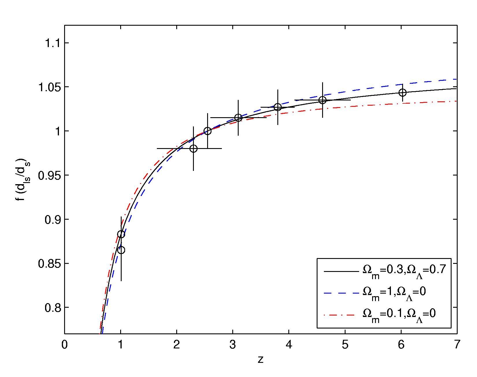
Figure 12.— Growth of the scaling factor $f(d_{ls}/d_{s})$ as a function of redshift, normalized so f=1 at $z=2.55$. Plotted lines are the expected ratio from the chosen specified cosmological model. The circles correspond to the multiple-image systems reproduced by our mass model, versus their real spectroscopic or photometric redshift. The data clearly follow well the relation predicted by the standard cosmological model. As can be seen, based on only one cluster and due to the low number of multiple images, it may be still hard to discriminate between different cosmologies solely with these data. With a sample of 25 CLASH clusters however, where most clusters are expected to have larger critical area and thus larger numbers of multiple-images spread over a large redshift range, we will be able to put statistically-significant constraints on the cosmological parameters, combining the information from all clusters together.

4.3. Brightest Cluster Galaxy

Due to the presence of the radial arc in its halo, we may also constrain the mass enclosed within the BCG, and the corresponding M/L ratio. We find that the BCG encloses a projected mass of $1.14\pm 0.3\times 10^{12}M_{\odot}$ within a radius of $\simeq 6\arcsec$ ($\simeq$19 kpc) after subtracting the interpolated smooth DM component ($\simeq 4.1\times 10^{12}M_{\odot}$ inside this aperture). For comparison, recent stellar velocity-dispersion measurements of the BCG in A383 yield $\sigma\simeq 450\pm 40$ at this radius (as read from Figure 2 in Newman et al. 2011), which translates to a projected mass of $0.89^{+0.22}_{-0.15}\times 10^{12}M_{\odot}$, in agreement with our result.

We measure the BCG flux in several optical ACS bands, to obtain an average B-band luminosity of $\simeq 8\pm 0.3\times 10^{10}L_{\odot}$, within the aperture of $\simeq 6\arcsec$ ($\simeq$19 kpc; fluxes were converted to luminosities using the LRG template described in Benítez et al. 2009a). This yields a typical $M/L_{B}$ of $\sim 14~{}(M/L)_{\odot}$ in this region, similar to other lensing based BCG masses in well-studied clusters (e.g., Gavazzi et al. 2003 for MS 2137-2353, Zitrin & Broadhurst 2009 for MACS J1149.5+2223, Limousin et al. 2008; Zitrin et al. 2010 for Abell 1703), though of course the degeneracy between the BCG DM halo and the overall subtracted smooth cluster halo is still unknown.

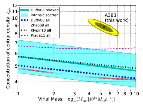
Figure 13.— The joint SL+WL NFW fit of A383 (data point with $1\sigma$ and $2\sigma$ confidence level contours) presented on the $c$–$M$ plane, compared to expectations from simulations. Overplotted are the expected $c$–$M$ relations and their 1$\sigma$ uncertainties, presented in Duffy et al. (2008) for their relaxed sample, scaled to $z_{c}=0.189$ (blue band). Also plotted are $c$–$M$ relations for the full-sample clusters from Duffy et al. (2008); Zhao et al. (2009); Klypin et al. (2010); Prada et al. (2011). As has been found for other observed clusters (e.g., Broadhurst et al. 2008; Oguri et al. 2009; Zitrin et al. 2010) A383 appears to have a higher concentration than simulated clusters with similar masses and redshifts. We note that the WL data used here are based on 1D analysis, while the concentration should be influenced by the triaxiality, and this result will be revised in our following WL paper using 2D analysis (Umetsu et al., in preparation).

4.4. Modeling Accuracy and Uncertainty

In general, since the deflection angle depends on the distance-redshift ratio ($D_{ls}/D_{s}$), the SL modeling uncertainty, particularly with regards to the mass profile, is primarily coupled to the redshift measurement accuracy of the multiple-systems. In A383, five systems at three different redshifts have spectroscopic measurements, while the four other systems found in this work importantly supply four more constraints on the mass profile. Our 16-band ACS/WFC3 imaging, allows us to derive robust photo-$z$’s for all multiply-lensed systems discussed in this work, which we verify by using both the BPZ method, and the LPZ method (§2).

Still, due to the low number of parameters in our modeling, which constitutes a huge advantage for finding multiple-images and producing efficiently well-constrained mass distributions, some local inaccuracy can be expected. Our best fit model for A383 reproduces all multiple-images described in this work within $\simeq 2.5\arcsec$ from their real location given their measured redshifts, aside from one image candidate belonging to system 9 (see §4.1) which is reproduced $\sim 4\arcsec$ from its real location. In addition, we note that in our best-fit model, constrained by all systems together, there is a slight offset of $\simeq 1\arcsec$ in the reproduced location of the radial arc, implying a slight inaccuracy in the BCG’s very inner mass profile in that model. Note however that this does not affect the result in §4.3, which was verified by complementary models in which the radial arc is very accurately reproduced (but the fit is overall somewhat poorer taking into account all other systems), thus reliably constraining the mass enclosed within the corresponding radius.

The average image-plane reproduction uncertainty of our best-fit model is $1.68\arcsec$ per image in total, with an image-plane $rms$ of $1.95\arcsec$ including all 27 multiply-lensed images. This image-plane $rms$ is, for example, higher than that reported recently by Newman et al. (2011) for A383 ($rms=0.27\arcsec$) based on only four systems in two different spectroscopic redshifts, but is typical to most parametric-method reconstructions, when many multiple-systems are present. For example, Broadhurst et al. (2005b) achieved an $rms$ of $3.2\arcsec$ per image for Abell 1689, and later Halkola et al. (2006) reported an $rms$ of $2.7\arcsec$ per image for that cluster, while Zitrin et al. (2009b) produced an $rms$ of $\simeq 2.5\arcsec$ for Cl0024. These values are comparable with our current model $rms$, taking into account the difference in the critical area.

In general, a higher number of parameters would supply a more accurate solution, however the efficiency of a model and the confidence in it decrease substantially as more parameters are added to the minimization procedure, especially if these are arbitrary non-physical parameters as may be the case in other (non-parametric) methods. We have shown here as well as in many previous examples (see also §3) that our method, with a minimum number of free parameters, built on simple physical considerations (see Zitrin et al. 2009b for full details), does a very good job in finding new multiply-lensed systems, and thus in constraining the deflection field, and accordingly, the mass distribution and profile.

5. Comparison to Numerical Simulations

We now compare our derived A383 mass distribution with cluster halos obtained from hydrodynamical simulations in the framework of the $\Lambda$CDM cosmology. The analysis we make here is inspired by the work of Meneghetti et al. (2011), where the Einstein ring sizes and the lensing cross sections of 12 massive MACS clusters modeled by Zitrin et al. (2011a) were compared with those expected from similar halos in the MareNostrum Universe cosmological simulation (Gottlöber & Yepes, 2007; Meneghetti et al., 2010a; Fedeli et al., 2010). This is a $500^{3}\;h^{-3}$Mpc³ volume filled with $1024^{3}$ DM and $1024^{3}$ gas particles, evolved in the framework of a cosmological model with $\Omega_{m}=0.3$, $\Omega_{\Lambda}=0.7$, and $\sigma_{8}=0.9$. More details about this simulation can be found in Gottlöber & Yepes (2007). For our comparison, we use halos extracted from the same cosmological box, for which the median Einstein ring sizes and the cross sections for giant arcs (defined as having length-to-width ratios larger than 7.5), were readily computed as in Meneghetti et al. (2011). To account for the lack of star formation in these simulations, we added to each halo a component mimicking the presence of a massive galaxy at the cluster center, following the method employed in Meneghetti et al. (2003). The galaxy was modeled with pseudo-isothermal mass distribution (see e.g. Donnarumma et al. 2011) with a velocity dispersion of $\sigma=300$ km/s and a cut-off radius of $23$ kpc.

We use the deflection angle maps of the A383 SL model presented here, and use them to perform a ray-tracing simulation. We stress that such a simulation is completely consistent with those performed for each simulated halo. A large number of artificial elliptical sources is used to populate the source plane at $z_{s}=2$, which are distributed on adaptive grids with increasing spatial resolution towards the caustics, in order to sample with greater accuracy the regions where sources are strongly magnified. By counting the sources that are lensed as giant arcs, we measure the lensing cross section, which is the area surrounding the caustics where sources must be located in order to produce images with length-to-width ratios larger than 7.5. The deflection angle maps also allow to measure the cluster median Einstein ring, defined as the median distance of the critical points from the cluster center. In the following discussion, we refer to the Einstein radius for sources at redshift $z_{s}=2$. Note also that the median Einstein radius is defined differently than the simple effective radius of the critical area which is usually used and was implemented throughout this work in order to compare to other results. In this section only, we use the $median$ Einstein radius, in order to be consistent with previous work based on these simulations and since it usually better correlates with the lensing cross-section (see Meneghetti et al. 2011).

By doing this analysis, we find that A383 has a median Einstein radius $\theta_{\rm med}=19.0\pm 1\arcsec$ , and a lensing cross section $\sigma=2.49\pm 0.9\times 10^{-3}\;h^{-2}$Mpc². Comparing these results with the distributions of $\theta_{\rm med}$ and $\sigma$ of halos with similar mass in the MareNostrum Universe, we find that A383 is a remarkably strong lens, given its relatively small mass. Indeed, the majority of simulated clusters with $6\times 10^{14}\leq M_{vir}\leq 7\times 10^{14}\;h^{-1}M_{\odot}$ have much smaller critical curves and cross sections. For example, the mean Einstein radius and lensing cross section of such sample are $8.9\arcsec$ and $5.6\times 10^{-4}\;h^{-2}$Mpc², respectively. The values measured for A383 exceed the maximal values measured in the simulations, which are $18.14\arcsec$ and $2.26\times 10^{-3}\;h^{-2}$Mpc², respectively. As an example, the distribution of median Einstein radii for simulated clusters is shown in Fig.14. As shown by Meneghetti et al. (2011), the lensing cross-section is tightly correlated to the median Einstein radius. We note also that each cluster in the MareNostrum Universe was projected along three independent lines-of-sight in order to account for possible projection effects, i.e. for including cases where clusters are seen nearly along their major axis. The largest Einstein radii and cross sections are indeed produced by clusters whose major axis is almost perfectly aligned to the line-of-sight. Nevertheless, it is difficult to find a cluster that matches the mass and the strong lensing efficiency of A383 among the simulated halos. Extending the upper mass limit of the simulated sample to $8\times 10^{14}\;h^{-1}M_{\odot}$, we find that only two cluster projections have Einstein radii and lensing cross sections larger than those measured for A383, which is still in the $>99\%$ tail of the corresponding distributions.

Meneghetti et al. (2010b) showed that the concentrations estimated from the projected mass distribution of strong lensing clusters are on-average biased high, i.e. they are higher than the corresponding concentrations measured from the three-dimensional cluster mass distributions (see also Hennawi et al. 2007). Such bias depends on the cluster mass, redshift, and lensing cross section. For a fixed mass and redshift, clusters with large lensing cross sections are typically affected by a more severe concentration bias. As done by Meneghetti et al. (2011), we use the MareNostrum Universe clusters to estimate a lower limit of the concentration bias for A383-like clusters. To do that, we select the numerically simulated halos with redshift and mass matching those of A383 and lensing cross section $\sigma>10^{-4}\;h^{-2}$Mpc². This limit was set in order to have a statistically significant sample of simulated halos. The median ratio of $c_{2D}/c_{3D}$ for these lenses is $\sim 1.35$. Thus, for objects with a lensing efficiency as high as in A383, the concentration measured from lensing is expected to be $>35\%$ higher than their true 3D-concentration. This expectation agrees well with a recent work by Morandi & Limousin (2011) estimating the triaxial shape of A383. Morandi & Limousin (2011) deduced by a joint analysis of X-ray and SL measurements (which are commensurate with our analysis), a concentration of $c_{vir}\sim 6.1$, while we obtained indeed a $44\%$ higher value in our 2D analysis, $c_{vir}\simeq 8.8$ (see §4.2).

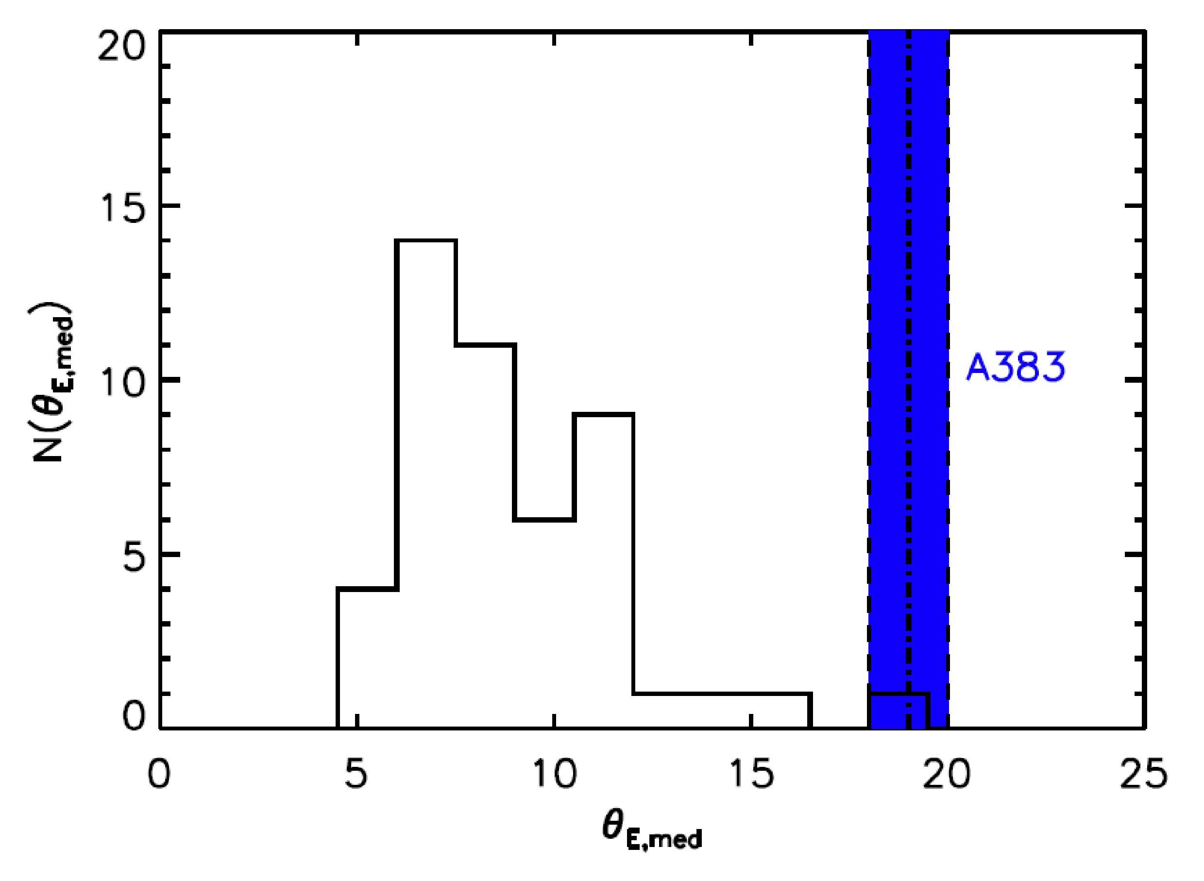
Figure 14.— Distribution of the $median$ Einstein radii of halos with $6\times 10^{14}\;h^{-1}M_{\odot}\leq M_{vir}\leq 7\times 10^{14}\;h^{-1}M_{\odot}$ extracted from the MareNostrum Universe snapshot at $z\sim 0.19$. The blue-shaded region shows the size of the median Einstein radius of A383 with its error-bar. See §5 for more details and the definition of the $median$ Einstein radius.

6. Summary

In this work we have presented a new detailed lensing analysis of the galaxy cluster A383 in multi-band ACS/WFC3 images. Our well-established modeling method (Broadhurst et al., 2005b; Zitrin et al., 2009b, 2010; Merten et al., 2011; Zitrin et al., 2011a, b, c) has identified 13 multiply-lensed images and candidates, so that in total 27 images of 9 different sources were incorporated to fully constrain the fit. Though more lensed candidates may generally be found in this lensing field with further careful effort, the resulting model is clearly fully constrained by these multiple systems.

The accurate photometric redshifts of the newly found multiple-systems enabled by the extensive multi-band HST imaging allow for the most secure lensing-based determination of the inner mass profile of A383 to date, through the cosmological lensing-distance ratio, and imply a mass profile of $d\log\Sigma/d\log r\simeq-0.6\pm 0.1$, similar to other well-known relaxed clusters, and in excellent agreement with WL analysis from wide-field Subaru data (Umetsu et al., in preparation, see also Figure 5). In addition, we note that our mass profile is generally consistent with a recent joint lensing, X-ray ,and kinematic analysis by Newman et al. (2011), out to at least twice the Einstein radius where our SL data apply.

In Figure 2 we plotted the critical curves along with the multiple images found and used in this work. For a source at $z_{s}=2.55$, the effective Einstein radius $r_{E}=16.3\pm 2\arcsec$, or $\simeq$52 kpc at the redshift of the cluster. This critical curve encloses a projected mass of $M=2.4\pm 0.2\times 10^{13}M_{\odot}$, in agreement with other published results (e.g., Smith et al. 2001; Newman et al. 2011).

We compared the properties of A383 with clusters of similar mass drawn from the MareNostrum Universe numerical simulation (see §5). We find that A383 is a remarkably strong lens, given its relatively small mass. The majority of simulated clusters $6\times 10^{14}\leq M_{vir}\leq 7\times 10^{14}\;h^{-1}M_{\odot}$ have much smaller critical curves and lensing cross sections. The largest Einstein radii and cross sections are produced by clusters whose major axis is almost perfectly aligned to the line-of-sight. Even with this taken into account, it is difficult to find a cluster that matches the mass and the strong lensing efficiency of A383 among the simulated halos, so that A383 lies at the $>99\%$ tail of the corresponding distributions (Figure 14). Accordingly, for objects with a lensing efficiency as high as in A383, the concentration measured from lensing is expected to be $>35\%$ higher than their true 3D-concentration, in agreement with recent results (e.g., Morandi & Limousin, 2011).

A383 is the first cluster observed and analyzed in the CLASH framework (see §1). As we have shown, despite the relatively small Einstein radius and correspondingly low number of multiply-lensed images, the remarkable 16 filter imaging allowed us to immediately uncover several new multiple-systems. With a statistical sample of 25 massive galaxy clusters being deeply imaged with HST, we should be able to test structure formation models with unprecedented precision.

References

- Anderson & Bedin (2010) Anderson, J., & Bedin, L. R. 2010, PASP, 122, 1035
- Arnouts et al. (1999) Arnouts, S., Cristiani, S., Moscardini, L., Matarrese, S., Lucchin, F., Fontana, A., & Giallongo, E. 1999, MNRAS, 310, 540
- Benítez (2000) Benítez, N. 2000, ApJ, 536, 571
- Benítez et al. (2004) Benítez, N., et al. 2004, ApJS, 150, 1
- Benítez et al. (2009a) —. 2009a, ApJ, 691, 241
- Benítez et al. (2009b) —. 2009b, ApJ, 692, L5
- Broadhurst et al. (2005a) Broadhurst, T., Takada, M., Umetsu, K., Kong, X., Arimoto, N., Chiba, M., & Futamase, T. 2005a, ApJ, 619, L143
- Broadhurst et al. (2008) Broadhurst, T., Umetsu, K., Medezinski, E., Oguri, M., & Rephaeli, Y. 2008, ApJ, 685, L9
- Broadhurst et al. (2005b) Broadhurst, T., et al. 2005b, ApJ, 621, 53
- Bruzual & Charlot (2003) Bruzual, G., & Charlot, S. 2003, MNRAS, 344, 1000
- Bullock et al. (2001) Bullock, J. S., Kolatt, T. S., Sigad, Y., Somerville, R. S., Kravtsov, A. V., Klypin, A. A., Primack, J. R., & Dekel, A. 2001, MNRAS, 321, 559
- Coe et al. (2010) Coe, D., Benítez, N., Broadhurst, T., & Moustakas, L. A. 2010, ApJ, 723, 1678
- Coe et al. (2006) Coe, D., Benítez, N., Sánchez, S. F., Jee, M., Bouwens, R., & Ford, H. 2006, AJ, 132, 926
- Collins et al. (2009) Collins, C. A., et al. 2009, Nature, 458, 603
- Corless & King (2009) Corless, V. L., & King, L. J. 2009, MNRAS, 396, 315
- Daddi et al. (2007) Daddi, E., et al. 2007, ApJ, 670, 156
- Daddi et al. (2009) —. 2009, ApJ, 694, 1517
- Donnarumma et al. (2011) Donnarumma, A., et al. 2011, A&A, 528, A73+
- Duffy et al. (2008) Duffy, A. R., Schaye, J., Kay, S. T., & Dalla Vecchia, C. 2008, MNRAS, 390, L64
- Duffy et al. (2010) Duffy, A. R., Schaye, J., Kay, S. T., Dalla Vecchia, C., Battye, R. A., & Booth, C. M. 2010, MNRAS, 405, 2161
- Evrard et al. (2002) Evrard, A. E., et al. 2002, ApJ, 573, 7
- Fedeli et al. (2010) Fedeli, C., Meneghetti, M., Gottlöber, S., & Yepes, G. 2010, A&A, 519, A91+
- Fioc & Rocca-Volmerange (1997) Fioc, M., & Rocca-Volmerange, B. 1997, A&A, 326, 950
- Gavazzi et al. (2003) Gavazzi, R., Fort, B., Mellier, Y., Pelló, R., & Dantel-Fort, M. 2003, A&A, 403, 11
- Gobat et al. (2011) Gobat, R., et al. 2011, A&A, 526, A133+
- Gottlöber & Yepes (2007) Gottlöber, S., & Yepes, G. 2007, ApJ, 664, 117
- Grogin et al. (2010) Grogin, N. A., Lucas, R., Golimowski, D., & Biretta, J. 2010, WFPC2 CTE for Extended Sources: I. Photometric Correction, Tech. rep.
- Halkola et al. (2006) Halkola, A., Seitz, S., & Pannella, M. 2006, MNRAS, 372, 1425
- Hennawi et al. (2007) Hennawi, J. F., Dalal, N., Bode, P., & Ostriker, J. P. 2007, ApJ, 654, 714
- Hildebrandt et al. (2010) Hildebrandt, H., et al. 2010, A&A, 523, A31+
- Huang et al. (2011) Huang, Z., Radovich, M., Grado, A., Puddu, E., Romano, A., Limatola, L., & Fu, L. 2011, arXiv, 1102.1837
- Ilbert et al. (2006) Ilbert, O., et al. 2006, A&A, 457, 841
- Ilbert et al. (2009) —. 2009, ApJ, 690, 1236
- Jee et al. (2009) Jee, M. J., et al. 2009, ApJ, 704, 672
- Jiménez-Teja & Benítez (2011) Jiménez-Teja, Y., & Benítez, N. 2011, arXiv, 1104.0683
- Jing & Suto (2000) Jing, Y. P., & Suto, Y. 2000, ApJ, 529, L69
- Jullo et al. (2010) Jullo, E., Natarajan, P., Kneib, J., D’Aloisio, A., Limousin, M., Richard, J., & Schimd, C. 2010, Science, 329, 924
- Kaiser & Squires (1993) Kaiser, N., & Squires, G. 1993, ApJ, 404, 441
- Klypin et al. (2010) Klypin, A., Trujillo-Gomez, S., & Primack, J. 2010, arXiv, 1002.3660
- Koekemoer et al. (2007) Koekemoer, A. M., et al. 2007, ApJS, 172, 196
- Lahav et al. (1991) Lahav, O., Lilje, P. B., Primack, J. R., & Rees, M. J. 1991, MNRAS, 251, 128
- Lemze et al. (2009) Lemze, D., Sadeh, S., & Rephaeli, Y. 2009, MNRAS, 397, 1876
- Liesenborgs et al. (2006) Liesenborgs, J., De Rijcke, S., & Dejonghe, H. 2006, MNRAS, 367, 1209
- Liesenborgs et al. (2007) Liesenborgs, J., de Rijcke, S., Dejonghe, H., & Bekaert, P. 2007, MNRAS, 380, 1729
- Liesenborgs et al. (2009) —. 2009, MNRAS, 397, 341
- Limousin et al. (2008) Limousin, M., et al. 2008, A&A, 489, 23
- Medezinski et al. (2011) Medezinski, E., Broadhurst, T., Umetsu, K., Benitez, N., & Taylor, A. 2011, arXiv, 1101.1955
- Medezinski et al. (2010) Medezinski, E., Broadhurst, T., Umetsu, K., Oguri, M., Rephaeli, Y., & Benítez, N. 2010, MNRAS, 405, 257
- Meneghetti et al. (2003) Meneghetti, M., Bartelmann, M., & Moscardini, L. 2003, MNRAS, 346, 67
- Meneghetti et al. (2010a) Meneghetti, M., Fedeli, C., Pace, F., Gottlöber, S., & Yepes, G. 2010a, A&A, 519, A90+
- Meneghetti et al. (2011) Meneghetti, M., Fedeli, C., Zitrin, A., Bartelmann, M., Broadhurst, T., Gottloeber, S., Moscardini, L., & Yepes, G. 2011, arXiv, 1103.0044
- Meneghetti et al. (2010b) Meneghetti, M., Rasia, E., Merten, J., Bellagamba, F., Ettori, S., Mazzotta, P., Dolag, K., & Marri, S. 2010b, A&A, 514, A93+
- Merten et al. (2009) Merten, J., Cacciato, M., Meneghetti, M., Mignone, C., & Bartelmann, M. 2009, A&A, 500, 681
- Merten et al. (2011) Merten, J., et al. 2011, arXiv, 1103.2772
- Morandi & Limousin (2011) Morandi, A., & Limousin, M. 2011, arXiv, 1108.0769
- Morandi et al. (2011) Morandi, A., Limousin, M., Rephaeli, Y., Umetsu, K., Barkana, R., Broadhurst, T., & Dahle, H. 2011, arXiv, 1103.0202
- Navarro et al. (1996) Navarro, J. F., Frenk, C. S., & White, S. D. M. 1996, ApJ, 462, 563
- Neto et al. (2007) Neto, A. F., et al. 2007, MNRAS, 381, 1450
- Newman et al. (2011) Newman, A. B., Treu, T., Ellis, R. S., & Sand, D. J. 2011, ApJ, 728, L39+
- Newman et al. (2009) Newman, A. B., Treu, T., Ellis, R. S., Sand, D. J., Richard, J., Marshall, P. J., Capak, P., & Miyazaki, S. 2009, ApJ, 706, 1078
- Oguri & Blandford (2009) Oguri, M., & Blandford, R. D. 2009, MNRAS, 392, 930
- Oguri et al. (2009) Oguri, M., et al. 2009, ApJ, 699, 1038
- Okabe et al. (2010) Okabe, N., Takada, M., Umetsu, K., Futamase, T., & Smith, G. P. 2010, PASJ, 62, 811
- Peebles (1985) Peebles, P. J. E. 1985, ApJ, 297, 350
- Postman et al. (2011) Postman, M., et al. 2011, ApJS submitted, arXiv, 1106.3328
- Prada et al. (2011) Prada, F., Klypin, A. A., Cuesta, A. J., Betancort-Rijo, J. E., & Primack, J. 2011, arXiv, 1104.5130
- Richard et al. (2011) Richard, J., Kneib, J., Ebeling, H., Stark, D., Egami, E., & Fiedler, A. K. 2011, arXiv, 1102.5092
- Rosati et al. (2009) Rosati, P., et al. 2009, A&A, 508, 583
- Sadeh & Rephaeli (2008) Sadeh, S., & Rephaeli, Y. 2008, MNRAS, 388, 1759
- Sand et al. (2008) Sand, D. J., Treu, T., Ellis, R. S., Smith, G. P., & Kneib, J. 2008, ApJ, 674, 711
- Sand et al. (2004) Sand, D. J., Treu, T., Smith, G. P., & Ellis, R. S. 2004, ApJ, 604, 88
- Schmidt & Allen (2007) Schmidt, R. W., & Allen, S. W. 2007, MNRAS, 379, 209
- Sereno et al. (2010) Sereno, M., Jetzer, P., & Lubini, M. 2010, MNRAS, 403, 2077
- Smith et al. (2001) Smith, G. P., Kneib, J., Ebeling, H., Czoske, O., & Smail, I. 2001, ApJ, 552, 493
- Smith et al. (2005) Smith, G. P., Kneib, J., Smail, I., Mazzotta, P., Ebeling, H., & Czoske, O. 2005, MNRAS, 359, 417
- Umetsu & Broadhurst (2008) Umetsu, K., & Broadhurst, T. 2008, ApJ, 684, 177
- Umetsu et al. (2011a) Umetsu, K., Broadhurst, T., Zitrin, A., Medezinski, E., Coe, D., & Postman, M. 2011a, arXiv, 1105.0444
- Umetsu et al. (2011b) Umetsu, K., Broadhurst, T., Zitrin, A., Medezinski, E., & Hsu, L. 2011b, ApJ, 729, 127
- Umetsu et al. (2010) Umetsu, K., Medezinski, E., Broadhurst, T., Zitrin, A., Okabe, N., Hsieh, B., & Molnar, S. M. 2010, ApJ, 714, 1470
- Wuyts et al. (2008) Wuyts, S., Labbé, I., Schreiber, N. M. F., Franx, M., Rudnick, G., Brammer, G. B., & van Dokkum, P. G. 2008, ApJ, 689, 653
- Zhao et al. (2003) Zhao, D. H., Jing, Y. P., Mo, H. J., & Börner, G. 2003, ApJ, 597, L9
- Zhao et al. (2009) —. 2009, ApJ, 707, 354
- Zhao (1996) Zhao, H. 1996, MNRAS, 278, 488
- Zitrin & Broadhurst (2009) Zitrin, A., & Broadhurst, T. 2009, ApJ, 703, L132
- Zitrin et al. (2011a) Zitrin, A., Broadhurst, T., Barkana, R., Rephaeli, Y., & Benítez, N. 2011a, MNRAS, 410, 1939
- Zitrin et al. (2011b) Zitrin, A., Broadhurst, T., Bartelmann, M., Rephaeli, Y., Oguri, M., Benítez, N., Hao, J., & Umetsu, K. 2011b, arXiv, 1105.2295
- Zitrin et al. (2011c) Zitrin, A., Broadhurst, T., Coe, D., Liesenborgs, J., Benítez, N., Rephaeli, Y., Ford, H., & Umetsu, K. 2011c, MNRAS, 413, 1753
- Zitrin et al. (2009a) Zitrin, A., Broadhurst, T., Rephaeli, Y., & Sadeh, S. 2009a, ApJ, 707, L102
- Zitrin et al. (2009b) Zitrin, A., et al. 2009b, MNRAS, 396, 1985
- Zitrin et al. (2010) —. 2010, MNRAS, 408, 1916