Single-parameter pumping in graphene
Abstract
We propose a quantum pump mechanism based on the particular properties of graphene, namely chirality and bipolarity. The underlying physics is the excitation of evanescent modes entering a potential barrier from one lead, while those from the other lead do not reach the driving region. This induces a large nonequilibrium current with electrons stemming from a broad range of energies, in contrast to the narrow resonances that govern the corresponding effect in semiconductor heterostructures. Moreover, the pump mechanism in graphene turns out to be robust, with a simple parameter dependence, which is beneficial for applications. Numerical results from a Floquet scattering formalism are complemented with analytical solutions for small to moderate driving.
pacs:
05.60.Gg, 73.40.Gk, 72.80.Vp, 72.40.+wI Introduction
Ratchets and pumps are devices in which spatio-temporal symmetry breaking turns an ac force without net bias into directed motion.Reimann (2002); Hänggi and Marchesoni (2009) If the time-dependence enters via only one parameter, the pump current vanishes in the adiabatic limit.Brouwer (1998) Therefore, single-parameter pumping requires non-equilibrium conditions enforced by driving beyond the adiabatic limit. This distinguishes single-parameter pumps from devices that operate with oriented work cycles, like turnstiles Switkes et al. (1999) or sluices.Vartiainen et al. (2007) Quantum pumps can be implemented with quantum dots in a two-dimensional electron gas (2DEG) driven by microwaves, Oosterkamp et al. (1998) surface-acoustic waves, Blumenthal et al. (2007) ac gate voltages DiCarlo et al. (2003); Kaestner et al. (2008); Fujiwara et al. (2008); Kaestner et al. (2009) or non-equilibrium noise.Khrapai et al. (2006) Here we propose a single-parameter pump based on the particular properties of graphene and show that these display a broad-band response, in contrast to 2DEG-based ratchets or pumps for which isolated resonances govern the effect.Oosterkamp et al. (1998); Strass et al. (2005); Khrapai et al. (2006)
Owing to the chiral and gapless nature of charge carriers in graphene, an electron hitting a potential step in this material may propagate forwards as a hole with opposite momentum.Klein (1927); Katsnelson et al. (2006) Due to this Klein tunneling it is difficult to confine electrons by electrostatic potentials. This phenomenon even extends to evanescent modes, i.e., modes that decay exponentially as a function of the barrier penetration. In graphene, electrons populating such modes can tunnel a large distance.Tworzydlo et al. (2006) This impediment to electrostatic confinement constitutes a drawback for many switching and sensing applications.
An inspection of present quantum pump designs suggests that graphene pumps would be negatively affected by this issue as well. For example, pumps have been realized with electrostatically defined double quantum dots in a 2DEG.Oosterkamp et al. (1998); Khrapai et al. (2006) In these experiments, a driving field induces dipole transitions of an electron from a metastable state below the Fermi energy in the, say, left dot to a metastable state in the right dot. Subsequently the electron will leave to the right lead, and an electron from the left lead will fill the empty state in the left dot. The emerging pump current therefore requires resonant conditions with a pair of energetically well-defined states, i.e., well isolated states with long life times, which do not exist in graphene.
Nevertheless, the alternative, graphene-specific mechanism identified here allows realizing highly efficient pumping, which may indeed outperform conventional devices. The large pump current emerges in the bipolar regime around the Dirac point. This is due to a scattering process where a whole continuum of evanescent modes is promoted into unidirectionally propagating states, which couple well to the leads because of chirality. Since this mechanism does not rely on intricate resonance conditions, but invokes graphene’s intrinsic features of bipolarity and chirality, the pump current is robust and displays a simple parameter dependence curve, as is desirable for electronic sensor applications.
This paper is organized as follows: In the next section we describe our proposal for a single-parameter pump and give typical values for length and energies scales. In Sec. III we introduce the Floquet scattering theory that applies to non-equilibrium pumping in graphene. We first present the general formalism and then consider the weak driving regime, where we derive analytical expressions for the one-photon transmission probability. In Sec. IV we present numerical results for the pumped current comparing the performances of graphene and a 2DEG pump. Moreover, we compare the numerics with the semiclassical approximation derived in the preceding section and find good agreement. The specific pumping mechanism by excitation of evanescent modes is explained in Sec. IV.1. Finally, we conclude in Sec. V.
II Description of the system
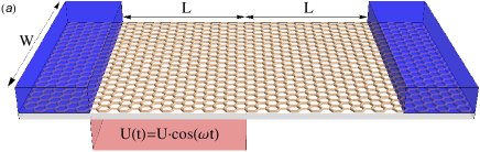
As a single-parameter pump setup, sketched in Fig. 1a, we consider a graphene ribbon of length and width attached to two metallic electron reservoirs, with its left half driven by a time-dependent gate. The driving by variation of only one parameter excludes the emergence of an adiabatic pump current.Brouwer (1998); Prada et al. (2009) However, considering that spatial symmetry is broken by the placement of the gate, a finite dc current arises in non-equilibrium conditions, which can be achieved by non-adiabatic driving. In order to assess the importance of graphene’s chirality and bipolarity in the non-adiabatic context, we contrast our results with those found for the corresponding setup of a 2DEG in a semiconductor heterostructure.
We assume that the sample sizes are smaller than the mean free path and that , so that the effects coming from the boundaries, electron-electron interactions and disorder play a minor role. Besides, we restrict ourselves to the low energy regime such that the Dirac approximation remains valid. Then, our quasi one-dimensional model contains three natural energy scales, namely the driving frequency , the driving amplitude , and the energy associated with the length of the device. Additionally, the leads’ Fermi momentum becomes a relevant scale in a 2DEG, since the contact resistance depends on its value. For graphene with Fermi velocity and , the latter is . For a 2DEG with the same geometry and effective mass (GaAs/AlGaAs), it is roughly four orders of magnitude smaller, . Driving beyond the adiabatic limit requires frequencies . Electrons can then absorb or emit photons, and after a short transient period, these excitations will establish a non-equilibrium population of the electronic states.
III Floquet scattering theory in graphene
A quantitative description of nonadiabatic charge transport is provided by Floquet scattering theory. Subsequently, we show that this theory provides the probability for an electron to be scattered from the left to the right lead under the absorption or emission of photons, and with it we can calculate the dc current.Kohler et al. (2005) In order to focus on the graphene-specific features, we will restrict ourselves to the zero temperature limit so that all electronic states below the Fermi energy are initially occupied.
III.1 General formalism
When scattered at a periodically time-dependent potential, an electron with initial energy may absorb or emit quanta of the driving field ( corresponds to emission), such that its final energy is . This is embodied in the decomposition of the transmission probability from the left to the right reservoir
| (1) |
The corresponding time-averaged dc current is given by the generalized Landauer formulaWagner and Sols (1999); Kohler et al. (2005)
| (2) |
where is the electron charge and is the Fermi-Dirac distribution. Spin and valley degeneracy of graphene is responsible for the prefactor , while accounts for the spin in a 2DEG. The application of Eq. (2) to graphene (or any other two-dimensional material) requires extending the summation to transverse momenta . For a driving field that breaks reflection symmetry, one generally finds . Then, even when the leads are in equilibrium such that , a net current may flow, and a pump current emerges,
| (3) |
where .
For the computation of the transmission probabilities we adopt the Floquet scattering formalism of Ref. Wagner, 1995 and consider electrons in two dimensions under the influence of a time-dependent potential described by the Hamiltonian
| (4) |
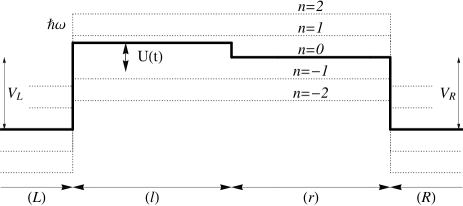
Here, comprises the kinetic energy and the static potential , while is the profile of the time-dependent potential with frequency . Since the potential is -independent, the transverse momentum is conserved and the problem becomes effectively one-dimensional. We assume that both the static potential and the driving profile are piecewise constant, and that outside the scattering region; see Fig. 2. For graphene, with the wavevector . The free solution with energy reads
| (5) |
where is positive and fulfills the dispersion relation , while is the sign of the corresponding current. The normalization has been chosen such that propagating waves have unit longitudinal current, . This is convenient since then the coefficients of a superposition become probability amplitudes. For evanescent solutions with imaginary longitudinal wavenumber , the current vanishes.
According to the Floquet theorem, the Schrödinger equation with a time-periodic Hamiltonian possesses a complete set of solutions with structure , where the Floquet state obeys the time-periodicity of the Hamiltonian and is the quasienergy. Here we are looking for Floquet scattering states, i.e., solutions of the Schrödinger equation that (i) are of Floquet structure and (ii) have an incoming plane wave as boundary condition. For clarity, we derive here only the transmission from left to right—for the opposite direction, it follows by simple re-labeling.
Condition (i) is equivalent to employing for the wavefunction in any of the four regions the ansatz . The time-periodic parts still have to be determined, while the quasienergy turns out to equal the energy of the incoming wave. Inserting into the Schrödinger equation of region yields for a partial differential equation which we solve by a separation ansatz. The resulting solutions
comply with the requirement of time-periodicity provided that the separation parameter is of integer value. The separation parameter labels all possible solutions and determines the time-averaged energy . The Bessel function of the first kind stems from the relation . Note that in the present case, is non-zero only in the driving region . The ansatz (III.1) has also been used to study photo-assisted tunneling in graphene.Trauzettel et al. (2007); *Trauzettel2007aE; Zeb et al. (2008); *AhsanZeb2008aE
Condition (ii) means that in region , the Floquet state consists of an incoming plane wave and a reflected part, , while in region , we have only an outgoing state, . With the normalization chosen for the free solutions (5), the coefficients of the latter superposition relate to the left-to-right transmission probability under absorption or emission of quanta according to
| (7) |
In the scattering regions and , the Floquet solution must be a superposition of the states (III.1), i.e., . The coefficients and follow from the requirement that the scattering states have to be continuous at any time. These matching conditions can be written as a set of linear equations, with the incoming wave appearing as inhomogenity. In matrix notation it reads
| (8) |
where denotes the incoming wave written as a 6-dimensional vector. The matrices are constructed from the wavefunctions (III.1) evaluated at the interfaces. They can be written efficiently as
| (9) |
where contains the wave matching condition at energy in the absence of driving. The matrix is a projector to region , constructed such that contains only wavefunctions from region . In particular, projects onto the driving region. Equation (8) fully determines the transmission and reflection amplitudes and . The tight-binding versionKohler et al. (2005) of this method is suitable for studying ac driving of smaller carbon-based conductors, such as ribbons with a size of only a few lattice constantsGu et al. (2009) or nanotubes.Foa Torres and Cuniberti (2009); Foa Torres et al. (2011) Via time-dependent density functional theory, it can be generalized to the presence of interactions.Stefanucci et al. (2008)
For electrons in a 2DEG with effective mass , the static Hamiltonian reads . Its free solutions are scalar fields, but since also their derivatives must be continuous, it is convenient to write them in spinor notation,
| (10) |
with the dispersion relation . The normalization is such that the first vector component has unit current, . With these ingredients, the Floquet scattering formalism can be directly applied to the 2DEG case.
III.2 Weak driving limit
The set of linear equations (8) can be solved analytically in the limit of small driving amplitudes or large frequencies, such that . We aim at finding analytical expressions for the one-photon transmission probabilities in terms of the static transmission for Klein tunneling at energy with respect to the top of a high barrier Katsnelson et al. (2006) of length ,
| (11) |
where . The semiclassical limit of the above relation is obtained by integration over fast oscillations, which yields . In order to relate these expressions to our formalism, we extract from the solution of Eq. (8) in the undriven limit, , the transmission amplitude by multiplication with the vector and obtain
| (12) |
Next we simplify Eq. (8) using for the Bessel functions the approximations , , while for . Thus, to first order in , only the Floquet indices remain. The resulting matrix can be inverted via the approximation , which provides and, thus,
| (13) |
The calculation of the elastic transmission up to leading order in is more tedious, but fortunately not required, because our Hamiltonian obeys time-reversal symmetry. Therefore, which implies that the elastic channel does not contribute to the pump current.Kohler et al. (2005)
Our numerical calculations will reveal that the relevant contributions to the pump current stem from modes that, in the absence of driving, are evanescent in the barrier region. For such modes, Eq. (13) can be connected to Eq. (12) in a simple way, because the modified source term in Eq. (13) has an invariant forward amplitude, . Although is not necessarily zero, it does not affect the transmission, since it merely redefines the reflection amplitude . As a result, the one-photon transmission, Eq. (13), becomes, besides a prefactor , identical to the static transmission (12) in the evanescent region,
| (14) |
For the evanescent modes entering from the right, the same reasoning lets us conclude that the waves decay exponentially and do not reach the driven region . Consequently, , and can be neglected. Then the net transmission appearing in Eq. (3) becomes
| (15) |
The magnitude of the correction reflects the fact that we have neglected the exponentally small transmission of the evanescent modes which decays with the imaginary wavenumber . Since , it follows that the maximal net transmission for evanescent waves is .
IV Non-adiabatic pump current
In the relevant weak driving regime , the absorption or emission probabilities are of the order [see Eq. (14)], so that . Moreover, for short and wide systems (width ), the total current takes the form of an integral over modes . Hence, the current (3) at a given Fermi energy (measured from the Dirac point of the barrier) can be expressed as
| (16) |
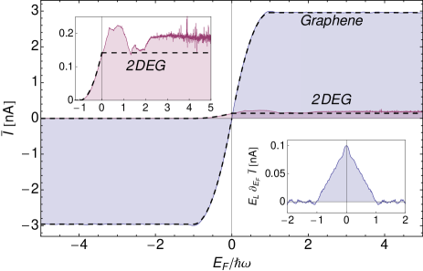
We compute numerically by wave-matching in Floquet space [see Eq. (8)]. Using typical parameters , , eV, meV (around GHz), we obtain the results shown in Fig. 3. As long as , the structure of the transmission for graphene depends only on the product , unlike for the 2DEG. Graphene develops a far larger pump current than a 2DEG, saturating to an - and -independent maximal value nA for , while the smaller pump current in the 2DEG case already saturates at . The semiclassical approximation described in Sec. III.2, valid for , yields
| (17) |
where the energy is the analogue of with replaced by the width . The corresponding calculation for a 2DEG provides the result
These approximations are plotted as dashed curves in Fig. 3. Unlike for graphene, the pump current in the 2DEG depends on the leads’ large Fermi momentum (around for gold electrodes), which has been assumed equal for both leads. The relative pump performance , assuming gold electrodes and GaAs/AlGaAs 2DEGs, is , i.e., the pump current in the graphene device is much larger than in the 2DEG device.
IV.1 Direction-dependent excitation of evanescent modes
In the following we show that the large and robust pump current of the graphene device stems from a mechanism whereby the ac field promotes evanescent modes from the left lead with probability into propagating modes, unlike evanescent modes from the right lead, which couple poorly to the driving region. In order to support this picture, we consider the differential response , shown in the lower inset of Fig. 3. It indicates that the main contribution to the current stems from the bipolar regime in the case of graphene, or from the gap boundary region in the case of the 2DEG. In the absence of driving, these energy ranges are populated by electronic modes that become evanescent in the barrier region. Whether modes are evanescent or propagating furthermore depends on their transverse momentum . Their response to driving is encoded in the function , which represents the differential response for a given mode with transverse momentum and total energy [see Eq. (16)].
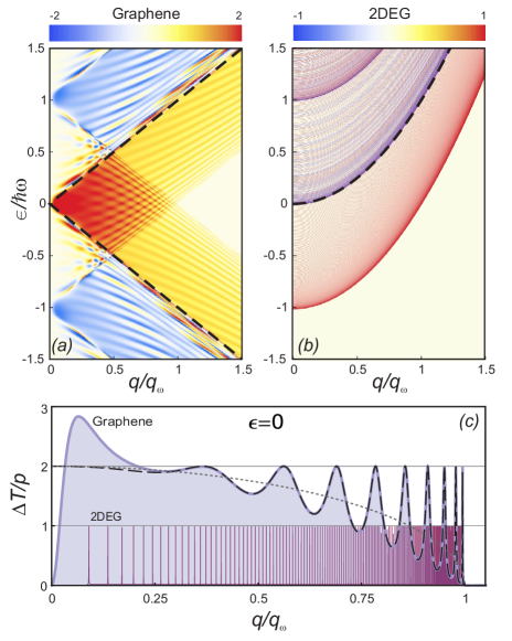
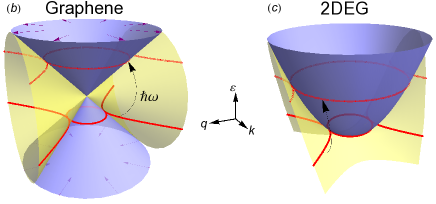
Figure 4 depicts for graphene and the 2DEG. In the 2DEG case, at each energy only a discrete set of resonant modes contributes to the pump effect. These resonances correspond, up to a shift of in energy, to quasibound levels in the static system, that form because of the velocity mismatch at the interface with the metallic leads, which results in strong confinement. The contact resistance increases with increasing Fermi momentum , and the resonances become increasingly narrow, resulting in a suppressed response of the 2DEG. By contrast, in graphene a broad range of modes contributes at all energies, and the response is particularly strong in a diamond-shaped region within the bipolar regime (red square in Fig. 4), in agreement with our earlier observation in Fig. 3. Graphene’s response does not exhibit sharp resonances due to the fact that, in the static case, carrier chirality prohibits their confinement, so that carriers in the graphene pump remain strongly coupled to the leads, even when they are driven far out of equilibrium. Instead, graphene’s response in Fig. 4(a) has features associated with the cone (dashed lines) and its replicas shifted by multiples of . For the weak driving considered here, only the two replicas at are visible. The first cone divides the modes entering the scattering region into two categories, propagating and evanescent: any incoming carrier in mode will become evanescent under the barrier if its energy fulfills , and will remain propagating otherwise. The other two cones determine whether carriers populate evanescent or propagating modes after absorption or emission of a single photon. Analogously, in the 2DEG the threshold between propagating and evanescent modes is found at , and under photon emission or absorption shifts to .
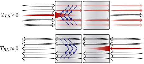
In both systems, it can now be seen that the main mechanism of charge transfer is established by a process whereby an evanescent mode coming from the left lead may get transmitted to the right by absorbing or emitting a photon, as long as in this process it jumps to an existing propagating mode that may travel into the right lead. An evanescent coming from the right, in contrast, first encounters the static region not covered by the gate, and so gets reflected with a high probability (see Fig. 5). This spatial asymmetry rectifies the carrier flux such that a net transport from left to right emerges.
In the 2DEG, when photon absorption is at resonance with a quasibound state, this process via evanescent modes yields a maximal value , but because the resonances are narrow the integrated current remains small. In graphene, on the other hand, all evanescent modes with exhibit a response , close to twice the optimal value of resonant evanescent modes in a 2DEG, but without the need to satisfy any resonance condition. The factor two comes from the two possible transitions to a propagating mode, by absorption but also by emission of a photon, i.e., it is directly related to bipolarity. Resonant conditions are not required because Klein tunneling in the propagating modes and macroscopic tunneling in evanescent modes keep the contacts always open; this is directly related to chirality. In combination, these two graphene-specific effects maximize the differential pump response around the Dirac point, and thus determine the robust characteristic features of the total pump current in Fig. 3.
V Conclusions
With this work, we have put forward a pump mechanism that makes use of the evanescent modes under a potential barrier in graphene. If an ac gate voltage acts upon the, say, left half of the barrier, electrons penetrating the barrier from the left lead are excited into propagating modes and, thus, will be scattered to the right lead. By contrast, electrons from the opposite side will reach the driving region only with exponentially small probability. This breaking of spatio-temporal symmetries induces surprisingly large non-adiabatic pump currents in the range of several nA, significantly larger than what has been observed so far with semiconductors. The main reason for this efficiency is that a whole range of evanescent modes is excited, while in the corresponding setup with a 2DEG, only isolated resonances contribute. Despite the large pump currents, the main effect stems from single-photon absorption, which allows one to obtain analytical results. Moreover, owing to current conservation, ratchets which are built by several pumps in series, exhibit identical operation characteristics (repetition of the element is therefore not desirable for practical implementations).
A further important observation is that the resulting pump current changes smoothly, symmetrically, and almost monotonically with the distance of the Fermi energy to the Dirac point. This behaviour is a direct consequence of bipolarity and, thus, particular to graphene pumps. As an application, it allows steering the dc current into a direction of choice by simply shifting the barrier height via a local dc gate voltage across the Dirac point. This effect can also be used to detect a static electric field by measuring the current in response to a small oscillating probe electric field, or detecting the amplitude of such an oscillating field when the static field is fixed to a moderately large value, beyond which the response flattens out.
Acknowledgements.
We acknowledge support by the CSIC JAE-Doc program and the Spanish Ministry of Science and Innovation through grants FIS2008-00124/FIS (P.S.-J), FIS2009-08744 (E.P.) and MAT2008-02626 (S.K.).References
- Reimann (2002) P. Reimann, Phys. Rep. 361, 57 (2002).
- Hänggi and Marchesoni (2009) P. Hänggi and F. Marchesoni, Rev. Mod. Phys. 81, 387 (2009).
- Brouwer (1998) P. W. Brouwer, Phys. Rev. B 58, R10135 (1998).
- Switkes et al. (1999) M. Switkes, C. M. Marcus, K. Campman, and A. C. Gossard, Science 283, 1905 (1999).
- Vartiainen et al. (2007) J. J. Vartiainen, M. Mottonen, J. P. Pekola, and A. Kemppinen, Appl. Phys. Lett. 90, 082102 (2007).
- Oosterkamp et al. (1998) T. H. Oosterkamp, T. Fujisawa, W. G. van der Wiel, K. Ishibashi, R. V. Hijman, S. Tarucha, and L. P. Kouwenhoven, Nature (London) 395, 873 (1998).
- Blumenthal et al. (2007) M. D. Blumenthal, B. Kaestner, L. Li, S. Giblin, T. J. B. M. Janssen, M. Pepper, D. Anderson, G. Jones, and D. A. Ritchie, Nature Phys. 3, 343 (2007).
- DiCarlo et al. (2003) L. DiCarlo, C. M. Marcus, and J. S. Harris, Jr., Phys. Rev. Lett. 91, 246804 (2003).
- Kaestner et al. (2008) B. Kaestner, V. Kashcheyevs, G. Hein, K. Pierz, U. Siegner, and H. W. Schumacher, Appl. Phys. Lett. 92, 192106 (2008).
- Fujiwara et al. (2008) A. Fujiwara, K. Nishiguchi, and Y. Ono, Appl. Phys. Lett. 92, 042102 (2008).
- Kaestner et al. (2009) B. Kaestner, C. Leicht, V. Kashcheyevs, K. Pierz, U. Siegner, and H. W. Schumacher, Appl. Phys. Lett. 94, 012106 (2009).
- Khrapai et al. (2006) V. S. Khrapai, S. Ludwig, J. P. Kotthaus, H. P. Tranitz, and W. Wegscheider, Phys. Rev. Lett. 97, 176803 (2006).
- Strass et al. (2005) M. Strass, P. Hänggi, and S. Kohler, Phys. Rev. Lett. 95, 130601 (2005).
- Klein (1927) O. Klein, Z. Phys. 53, 157 (1927).
- Katsnelson et al. (2006) M. I. Katsnelson, K. S. Novoselov, and A. K. Geim, Nature Phys. 2, 620 (2006).
- Tworzydlo et al. (2006) J. Tworzydlo, B. Trauzettel, M. Titov, A. Rycerz, and C. W. J. Beenakker, Phys. Rev. Lett. 96, 246802 (2006).
- Prada et al. (2009) E. Prada, P. San-Jose, and H. Schomerus, Phys. Rev. B 80, 245414 (2009).
- Kohler et al. (2005) S. Kohler, J. Lehmann, and P. Hänggi, Phys. Rep. 406, 379 (2005).
- Wagner and Sols (1999) M. Wagner and F. Sols, Phys. Rev. Lett. 83, 4377 (1999).
- Wagner (1995) M. Wagner, Phys. Rev. A 51, 798 (1995).
- Trauzettel et al. (2007) B. Trauzettel, Y. M. Blanter, and A. F. Morpurgo, Phys. Rev. B 75, 035305 (2007).
- Trauzettel et al. (2011) B. Trauzettel, Y. M. Blanter, and A. F. Morpurgo, Phys. Rev. B 83, 159902(E) (2011).
- Zeb et al. (2008) M. A. Zeb, K. Sabeeh, and M. Tahir, Phys. Rev. B 78, 165420 (2008).
- Zeb et al. (2009) M. A. Zeb, K. Sabeeh, and M. Tahir, Phys. Rev. B 79, 089903(E) (2009).
- Gu et al. (2009) Y. Gu, Y. H. Yang, J. Wang, and K. S. Chan, J. Phys.: Condens. Matter 21, 405301 (2009).
- Foa Torres and Cuniberti (2009) L. E. F. Foa Torres and G. Cuniberti, C. R. Physique 10, 297 (2009).
- Foa Torres et al. (2011) L. E. F. Foa Torres, H. L. Calvo, C. G. Rocha, and G. Cuniberti, Appl. Phys. Lett. 99, 092102 (2011).
- Stefanucci et al. (2008) G. Stefanucci, S. Kurth, A. Rubio, and E. K. U. Gross, Phys. Rev. B 77, 075339 (2008).