Least-Squares Independence Regression for Non-Linear Causal Inference under Non-Gaussian Noise

Abstract

The discovery of non-linear causal relationship under additive non-Gaussian noise models has attracted considerable attention recently because of their high flexibility. In this paper, we propose a novel causal inference algorithm called least-squares independence regression (LSIR). LSIR learns the additive noise model through the minimization of an estimator of the squared-loss mutual information between inputs and residuals. A notable advantage of LSIR over existing approaches is that tuning parameters such as the kernel width and the regularization parameter can be naturally optimized by cross-validation, allowing us to avoid overfitting in a data-dependent fashion. Through experiments with real-world datasets, we show that LSIR compares favorably with a state-of-the-art causal inference method.

1 Introduction

Learning causality from data is one of the important challenges in the artificial intelligence, statistics, and machine learning communities (Pearl, 2000). A traditional method of learning causal relationship from observational data is based on the linear-dependence Gaussian-noise model (Geiger and Heckerman, 1994). However, the linear-Gaussian assumption is too restrictive and may not be fulfilled in practice. Recently, non-Gaussianity and non-linearity have been shown to be beneficial in causal inference, allowing one to break symmetry between observed variables (Shimizu et al., 2006; Hoyer et al., 2009). Since then, much attention has been paid to the discovery of non-linear causal relationship through non-Gaussian noise models (Mooij et al., 2009).

In the framework of non-linear non-Gaussian causal inference, the relation between a cause $X$ and an effect $Y$ is assumed to be described by $Y=f(X)+E$, where $f$ is a non-linear function and $E$ is non-Gaussian additive noise which is independent of the cause $X$. Given two random variables $X$ and $X^{\prime}$, the causal direction between $X$ and $X^{\prime}$ is decided based on a hypothesis test of whether the model $X^{\prime}=f(X)+E$ or the alternative model $X=f^{\prime}(X^{\prime})+E^{\prime}$ fits the data well—here, the goodness of fit is measured by independence between inputs and residuals (i.e., estimated noise). Hoyer et al. (2009) proposed to learn the functions $f$ and $f^{\prime}$ by the Gaussian process (GP) (Bishop, 2006), and evaluate the independence between the inputs and the residuals by the Hilbert-Schmidt independence criterion (HSIC) (Gretton et al., 2005).

However, since standard regression methods such as GP are designed to handle Gaussian noise, they may not be suited for discovering causality in the non-Gaussian additive noise formulation. To cope with this problem, a novel regression method called HSIC regression (HSICR) has been introduced recently (Mooij et al., 2009). HSICR learns a function so that the dependence between inputs and residuals is directly minimized based on HSIC. Since HSICR does not impose any parametric assumption on the distribution of additive noise, it is suited for non-linear non-Gaussian causal inference. Indeed, HSICR was shown to outperform the GP-based method in experiments (Mooij et al., 2009).

However, HSICR still has limitations for its practical use. The first weakness of HSICR is that the kernel width of HSIC needs to be determined manually. Since the choice of the kernel width heavily affects the sensitivity of the independence measure (Fukumizu et al., 2009), lack of systematic model selection strategies is critical in causal inference. Setting the kernel width to the median distance between sample points is a popular heuristic in kernel methods (Schölkopf and Smola, 2002), but this does not always perform well in practice. Another limitation of HSICR is that the kernel width of the regression model is fixed to the same value as HSIC. This crucially limits the flexibility of function approximation in HSICR.

To overcome the above weaknesses, we propose an alternative regression method called least-squares independence regression (LSIR). As HSICR, LSIR also learns a function so that the dependence between inputs and residuals is directly minimized. However, a difference is that, instead of HSIC, LSIR adopts an independence criterion called least-squares mutual information (LSMI) (Suzuki et al., 2009), which is a consistent estimator of the squared-loss mutual information (SMI) with the optimal convergence rate. An advantage of LSIR over HSICR is that tuning parameters such as the kernel width and the regularization parameter can be naturally optimized through cross-validation (CV) with respect to the LSMI criterion.

Furthermore, we propose to determine the kernel width of the regression model based on CV with respect to SMI itself. Thus, the kernel width of the regression model is determined independent of that in the independence measure. This allows LSIR to have higher flexibility in non-linear causal inference than HSICR. Through experiments with real-world datasets, we demonstrate the superiority of LSIR.

2 Dependence Minimizing Regression by LSIR

In this section, we formulate the problem of dependence minimizing regression and propose a novel regression method, least-squares independence regression (LSIR).

2.1 Problem Formulation

Suppose random variables $X\in\mathbb{R}$ and $Y\in\mathbb{R}$ are connected by the following additive noise model (Hoyer et al., 2009):

$$Y=f(X)+E,$$

where $f:\mathbb{R}\rightarrow\mathbb{R}$ is some non-linear function and $E\in\mathbb{R}$ is a zero-mean random variable independent of $X$. The goal of dependence minimizing regression is, from i.i.d. paired samples $\{(x_{i},y_{i})\}_{i=1}^{n}$, to obtain a function $\widehat{f}$ such that input $X$ and estimated additive noise $\widehat{E}=Y-\widehat{f}(X)$ are independent.

Let us employ a linear model for dependence minimizing regression:

$$f_{{\bm{\beta}}}(x)=\sum_{l=1}^{m}\beta_{l}\psi_{l}(x)={\bm{\beta}}^{\top}{\bm{\psi}}(x),$$ (1)

where $m$ is the number of basis functions, ${\bm{\beta}}=(\beta_{1},\ldots,\beta_{m})^{\top}$ are regression parameters, ^⊤ denotes the transpose, and ${\bm{\psi}}(x)=(\psi_{1}(x),\ldots,\psi_{m}(x))^{\top}$ are basis functions. We use the Gaussian basis function in our experiments:

$$\psi_{l}(x)=\exp\left(-\frac{(x-c_{l})^{2}}{2\tau^{2}}\right),$$

where $c_{l}$ is the Gaussian center chosen randomly from $\{x_{i}\}_{i=1}^{n}$ without overlap and $\tau$ is the kernel width.

In dependence minimization regression, we learn the regression parameter ${\bm{\beta}}$ as

$$\min_{{\bm{\beta}}}\left[I(X,\widehat{E})+\frac{\gamma}{2}{\bm{\beta}}^{\top}{\bm{\beta}}\right],$$

where $I(X,\widehat{E})$ is some measure of independence between $X$ and $\widehat{E}$, and $\gamma\geq 0$ is the regularization parameter for avoiding overfitting.

In this paper, we use the squared-loss mutual information (SMI) (Suzuki et al., 2009) as our independence measure:

$$\textnormal{SMI}(X,\widehat{E}) =\frac{1}{2}\iint\left(\frac{p(x,\widehat{e})}{p(x)p(\widehat{e})}-1\right)^{2}p(x)p(\widehat{e})\textnormal{d}x\textnormal{d}\widehat{e}.$$

$\textnormal{SMI}(X,\widehat{E})$ is the Pearson divergence (Pearson, 1900) from $p(x,\widehat{e})$ to $p(x)p(\widehat{e})$, and it vanishes if and only if $p(x,\widehat{e})$ agrees with $p(x)p(\widehat{e})$, i.e., $X$ and $\widehat{E}$ are independent. Note that ordinary mutual information (MI) (Cover and Thomas, 2006),

$$\textnormal{MI}(X,\widehat{E}) =\iint p(x,\widehat{e})\log\frac{p(x,\widehat{e})}{p(x)p(\widehat{e})}\textnormal{d}x\textnormal{d}\widehat{e},$$ (2)

corresponds to the Kullback-Leibler divergence (Kullback and Leibler, 1951) from $p(x,\widehat{e})$ and $p(x)p(\widehat{e})$, and it can also be used as an independence measure. Nevertheless, we adhere to using SMI since it allows us to obtain an analytic-form estimator, as explained below.

2.2 Estimation of Squared-Loss Mutual Information

SMI cannot be directly computed since it contains unknown densities $p(x,\widehat{e})$, $p(x)$, and $p(\widehat{e})$. Here, we briefly review an SMI estimator called least-squares mutual information (LSMI) (Suzuki et al., 2009).

Since density estimation is known to be a hard problem (Vapnik, 1998), avoiding density estimation is critical for obtaining better SMI approximators (Kraskov et al., 2004). A key idea of LSMI is to directly estimate the density ratio:

$$r(x,\widehat{e})=\frac{p(x,\widehat{e})}{p(x)p(\widehat{e})},$$

without going through density estimation of $p(x,\widehat{e})$, $p(x)$, and $p(\widehat{e})$.

In LSMI, the density ratio function $r(x,\widehat{e})$ is directly modeled by the following linear model:

$$r_{{\bm{\alpha}}}(x,\widehat{e})=\sum_{l=1}^{b}\alpha_{l}\varphi_{l}(x,\widehat{e})={\bm{\alpha}}^{\top}{\bm{\varphi}}(x,\widehat{e}),$$ (3)

where $b$ is the number of basis functions, ${\bm{\alpha}}=(\alpha_{1},\ldots,\alpha_{b})^{\top}$ are parameters, and ${\bm{\varphi}}(x,\widehat{e})=(\varphi_{1}(x,\widehat{e}),\ldots,\varphi_{b}(x,\widehat{e}))^{\top}$ are basis functions. We use the Gaussian basis function:

$$\varphi_{l}(x,\widehat{e})=\exp\left(-\frac{(x-u_{l})^{2}+(\widehat{e}-\widehat{v}_{l})^{2}}{2\sigma^{2}}\right),$$

where $(u_{l},\widehat{v}_{l})$ is the Gaussian center chosen randomly from $\{(x_{i},\widehat{e}_{i})\}_{i=1}^{n}$ without replacement, and $\sigma$ is the kernel width.

The parameter ${\bm{\alpha}}$ in the model $r_{{\bm{\alpha}}}(x,\widehat{e})$ is learned so that the following squared error $J_{0}({\bm{\alpha}})$ is minimized:

$$J_{0}({\bm{\alpha}}) =\frac{1}{2}\iint(r_{{\bm{\alpha}}}(x,\widehat{e})-r(x,\widehat{e}))^{2}p(x)p(\widehat{e})\textnormal{d}x\textnormal{d}\widehat{e}$$

$$=\frac{1}{2}\iint r_{{\bm{\alpha}}}(x,\widehat{e})p(x)p(\widehat{e})\textnormal{d}x\textnormal{d}\widehat{e}-\iint r_{{\bm{\alpha}}}(x,\widehat{e})p(x,\widehat{e})\textnormal{d}x\textnormal{d}\widehat{e}+C,$$

where $C$ is a constant independent of ${\bm{\alpha}}$ and therefore can be safely ignored. Let us denote the first two terms by $J({\bm{\alpha}})$:

$$J({\bm{\alpha}})=J_{0}({\bm{\alpha}})-C=\frac{1}{2}{\bm{\alpha}}^{\top}{\bm{H}}{\bm{\alpha}}-{\bm{h}}^{\top}{\bm{\alpha}},$$ (4)

where

$${\bm{H}} =\iint{\bm{\varphi}}(x,\widehat{e}){\bm{\varphi}}(x,\widehat{e})^{\top}p(x)p(\widehat{e})\textnormal{d}x\textnormal{d}\widehat{e},$$

$${\bm{h}} =\iint{\bm{\varphi}}(x,\widehat{e})p(x,\widehat{e})\textnormal{d}x\textnormal{d}\widehat{e}.$$

Approximating the expectations in ${\bm{H}}$ and ${\bm{h}}$ by empirical averages, we obtain the following optimization problem:

$$\tilde{{\bm{\alpha}}}=\mathop{\text{argmin}}_{{\bm{\alpha}}}\Bigl{[}\frac{1}{2}{\bm{\alpha}}^{\top}\widehat{{\bm{H}}}{\bm{\alpha}}-\widehat{{\bm{h}}}^{\top}{\bm{\alpha}}+\lambda{\bm{\alpha}}^{\top}{\bm{\alpha}}\Bigr{]},$$

where a regularization term $\lambda{\bm{\alpha}}^{\top}{\bm{\alpha}}$ is included for avoiding overfitting, and

$$\widehat{{\bm{H}}} =\frac{1}{n^{2}}\sum_{i,j=1}^{n}{\bm{\varphi}}(x_{i},\widehat{e}_{j}){\bm{\varphi}}(x_{i},\widehat{e}_{j})^{\top},$$

$$\widehat{{\bm{h}}} =\frac{1}{n}\sum_{i=1}^{n}{\bm{\varphi}}(x_{i},\widehat{e}_{i}).$$

Differentiating the above objective function with respect to ${\bm{\alpha}}$ and equating it to zero, we can obtain an analytic-form solution:

$$\widehat{{\bm{\alpha}}}=(\widehat{{\bm{H}}}+\lambda{\bm{I}}_{b})^{-1}\widehat{{\bm{h}}},$$ (5)

where ${\bm{I}}_{b}$ denotes the $b$-dimensional identity matrix. It was shown that LSMI is consistent under mild assumptions and it achieves the optimal convergence rate (Kanamori et al., 2009).

Given a density ratio estimator $\widehat{r}=r_{\widehat{{\bm{\alpha}}}}$, SMI can be simply approximated as follows (Suzuki and Sugiyama, 2010):

$$\widehat{\textnormal{SMI}}(X,\widehat{E}) =\frac{1}{n}\sum_{i=1}^{n}\widehat{r}(x_{i},\widehat{e}_{i})-\frac{1}{2n^{2}}\sum_{i=1}^{n}\widehat{r}(x_{i},\widehat{e}_{i})^{2}-\frac{1}{2}$$

$$=\widehat{{\bm{h}}}^{\top}\widehat{{\bm{\alpha}}}-\frac{1}{2}\widehat{{\bm{\alpha}}}^{\top}\widehat{{\bm{H}}}\widehat{{\bm{\alpha}}}-\frac{1}{2}.$$ (6)

2.3 Model Selection in LSMI

LSMI contains three tuning parameters: the number of basis functions $b$, the kernel width $\sigma$, and the regularization parameter $\lambda$. In our experiments, we fix $b=\min(200,n)$, and choose $\sigma$ and $\lambda$ by cross-validation (CV) with grid search as follows. First, the samples ${\cal Z}=\{z_{i}\;|\;z_{i}=(x_{i},\widehat{e}_{i})\}_{i=1}^{n}$ are divided into $K$ disjoint subsets $\{{\cal Z}_{k}\}_{k=1}^{K}$ of (approximately) the same size (we set $K=2$ in experiments). Then, an estimator $\widehat{{\bm{\alpha}}}_{{\cal Z}_{k}}$ is obtained using ${\cal Z}\backslash{\cal Z}_{k}$ (i.e., without ${\cal Z}_{k}$), and the approximation error for the hold-out samples ${\cal Z}_{k}$ is computed as

$$J_{{\cal Z}_{k}}^{(K\text{-CV})}=\frac{1}{2}\widehat{{\bm{\alpha}}}_{{\cal Z}_{k}}^{\top}\widehat{{\bm{H}}}_{{\cal Z}_{k}}\widehat{{\bm{\alpha}}}_{{\cal Z}_{k}}-\widehat{{\bm{h}}}_{{\cal Z}_{k}}^{\top}\widehat{{\bm{\alpha}}}_{{\cal Z}_{k}},$$

where, for $|{\cal Z}_{k}|$ being the number of samples in the subset ${\cal Z}_{k}$,

$$\widehat{{\bm{H}}}_{{\cal Z}_{k}} =\frac{1}{|{\cal Z}_{k}|^{2}}\sum_{x,\widehat{e}\in{\cal Z}_{k}}{\bm{\varphi}}(x,\widehat{e}){\bm{\varphi}}(x,\widehat{e})^{\top},$$

$$\widehat{{\bm{h}}}_{{\cal Z}_{k}} =\frac{1}{|{\cal Z}_{k}|}\sum_{(x,\widehat{e})\in{\cal Z}_{k}}{\bm{\varphi}}(x,\widehat{e}).$$

This procedure is repeated for $k=1,\ldots,K$, and its average $J^{(K\text{-CV})}$ is outputted as

$$J^{(K\text{-CV})}=\frac{1}{K}\sum_{k=1}^{K}J_{{\cal Z}_{k}}^{(K\text{-CV})}.$$ (7)

We compute $J^{(K\text{-CV})}$ for all model candidates (the kernel width $\sigma$ and the regularization parameter $\lambda$ in the current setup), and choose the model that minimizes $J^{(K\text{-CV})}$. Note that $J^{(K\text{-CV})}$ is an almost unbiased estimator of the objective function (4), where the almost-ness comes from the fact that the number of samples is reduced in the CV procedure due to data splitting (Schölkopf and Smola, 2002).

The LSMI algorithm is summarized in Figure 1.

Input: $\{(x_{i},\widehat{e}_{i})\}_{i=1}^{n}$, $\{\sigma_{i}\}_{i=1}^{p}$, and $\{\lambda_{j}\}_{j=1}^{q}$ Output: LSMI parameter $\widehat{{\bm{\alpha}}}$ Compute CV score for $\{\sigma_{i}\}_{i=1}^{p}$ and $\{\lambda_{j}\}_{j=1}^{q}$ by Eq.(7); Choose $\widehat{\sigma}$ and $\widehat{\lambda}$ that minimize the CV score; Compute $\widehat{{\bm{\alpha}}}$ by Eq.(5) with $\widehat{\sigma}$ and $\widehat{\lambda}$;

Figure 1: Pseudo code of the LSMI algorithm with CV.

2.4 Least-Squares Independence Regression

Given the SMI estimator (6), our next task is to learn the parameter ${\bm{\beta}}$ in the regression model (1) as

$$\widehat{{\bm{\beta}}}=\mathop{\text{argmin}}_{{\bm{\beta}}}\left[\widehat{\textnormal{SMI}}(X,\widehat{E})+\frac{\gamma}{2}{\bm{\beta}}^{\top}{\bm{\beta}}\right].$$

We call this method least-squares independence regression (LSIR).

For regression parameter learning, we simply employ a gradient descent method:

$${\bm{\beta}}\longleftarrow{\bm{\beta}}-\eta\left(\frac{\partial\widehat{\textnormal{SMI}}(X,\widehat{E})}{\partial{\bm{\beta}}}+\gamma{\bm{\beta}}\right),$$ (8)

where $\eta$ is a step size which may be chosen in practice by some approximate line search method such as Armijo’s rule (Patriksson, 1999).

The partial derivative of $\widehat{\textnormal{SMI}}(X,\widehat{E})$ with respect to ${\bm{\beta}}$ can be approximately expressed as

$$\frac{\partial\widehat{\textnormal{SMI}}(X,\widehat{E})}{\partial{\bm{\beta}}}\approx\sum_{l=1}^{b}\widehat{\alpha}_{l}\frac{\partial\widehat{h}_{l}}{\partial{\bm{\beta}}}-\frac{1}{2}\sum_{l,l^{\prime}=1}^{b}\widehat{\alpha}_{l}\widehat{\alpha}_{l}^{\prime}\frac{\partial\widehat{H}_{l,l^{\prime}}}{\partial{\bm{\beta}}},$$

where

$$\frac{\partial\widehat{h}_{l}}{\partial{\bm{\beta}}} =\frac{1}{n}\sum_{i=1}^{n}\frac{\partial\varphi_{l}(x_{i},\widehat{e}_{i})}{\partial{\bm{\beta}}},$$

$$\frac{\partial\widehat{H}_{l,l^{\prime}}}{\partial{\bm{\beta}}} =\frac{1}{n^{2}}\sum_{i,j=1}^{n}\Biggl{(}\frac{\partial\varphi_{l}(x_{i},\widehat{e}_{j})}{\partial{\bm{\beta}}}\varphi_{l^{\prime}}(x_{j},\widehat{e}_{i})+\varphi_{l}(x_{i},\widehat{e}_{j})\frac{\partial\varphi_{l}(x_{j},\widehat{e}_{i})}{\partial{\bm{\beta}}}\Biggr{)},$$

$$\frac{\partial\varphi_{l}(x,\widehat{e})}{\partial{\bm{\beta}}} =-\frac{1}{2\sigma^{2}}\varphi_{l}(x,\widehat{e})(\widehat{e}-\widehat{v}_{l}){\bm{\psi}}(x).$$

In the above derivation, we ignored the dependence of ${\bm{\beta}}$ on $\widehat{e}_{i}$. It is possible to exactly compute the derivative in principle, but we use this approximated expression since it is computationally efficient.

We assumed that the mean of the noise $E$ is zero. Taking into account this, we modify the final regressor as

$$\widehat{f}(x)=f_{\widehat{{\bm{\beta}}}}(x)+\frac{1}{n}\sum_{i=1}^{n}\left(y_{i}-f_{\widehat{{\bm{\beta}}}}(x_{i})\right).$$

2.5 Model Selection in LSIR

LSIR contains three tuning parameters—the number of basis functions $m$, the kernel width $\tau$, and the regularization parameter $\gamma$. In our experiments, we fix $m=\min(200,n)$, and choose $\tau$ and $\gamma$ by CV with grid search as follows. First, the samples ${\cal Z}=\{z_{i}\;|\;z_{i}=(x_{i},\widehat{e}_{i})\}_{i=1}^{n}$ are divided into $T$ disjoint subsets $\{{\cal Z}_{t}\}_{t=1}^{T}$ of (approximately) the same size (we set $T=2$ in experiments). Then, an estimator $\widehat{{\bm{\beta}}}_{{\cal Z}_{t}}$ is obtained using ${\cal Z}\backslash{\cal Z}_{t}$ (i.e., without ${\cal Z}_{t}$), and the independence criterion for the hold-out samples ${\cal Z}_{t}$ is computed as

$$\widehat{I}_{{\cal Z}_{t}}^{(T\text{-CV})}=\widehat{{\bm{h}}}_{{\cal Z}_{t}}^{\top}\widehat{{\bm{\alpha}}}_{{\cal Z}_{t}}-\frac{1}{2}\widehat{{\bm{\alpha}}}_{{\cal Z}_{t}}^{\top}\widehat{{\bm{H}}}_{{\cal Z}_{t}}\widehat{{\bm{\alpha}}}_{{\cal Z}_{t}}-\frac{1}{2}.$$

This procedure is repeated for $t=1,\ldots,T$, and its average $\widehat{I}^{(T\text{-CV})}$ is computed as

$$\widehat{I}^{(T\text{-CV})}=\frac{1}{T}\sum_{t=1}^{T}\widehat{I}_{{\cal Z}_{t}}^{(T\text{-CV})}.$$ (9)

We compute $\widehat{I}^{(T\text{-CV})}$ for all model candidates (the kernel width $\tau$ and the regularization parameter $\gamma$ in the current setup), and choose the model that minimizes $\widehat{I}^{(T\text{-CV})}$.

The LSIR algorithm is summarized in Figure 2. A MATLAB^® implementation of LSIR is available from

‘http://sugiyama-www.cs.titech.ac.jp/$\tilde{~{}}$yamada/lsir.html’.

Input: $\{(x_{i},y_{i})\}_{i=1}^{n}$, $\{\tau_{i}\}_{i=1}^{p}$, and $\{\gamma_{j}\}_{j=1}^{q}$ Output: LSIR parameter $\widehat{{\bm{\beta}}}$ Compute CV score for all $\{\tau_{i}\}_{i=1}^{p}$ and $\{\gamma_{j}\}_{j=1}^{q}$ by Eq.(9); Choose $\widehat{\tau}$ and $\widehat{\gamma}$ that minimize the CV score; Compute $\widehat{{\bm{\beta}}}$ by gradient descent (8) with $\widehat{\tau}$ and $\widehat{\gamma}$;

Figure 2: Pseudo code of the LSIR algorithm with CV.

3 Causal Direction Inference by LSIR

In the previous section, we gave a dependence minimizing regression method, LSIR, that is equipped with CV for model selection. In this section, following Hoyer et al. (2009), we explain how LSIR can be used for causal direction inference.

Our final goal is, given i.i.d. paired samples $\{(x_{i},y_{i})\}_{i=1}^{n}$, to determine whether $X$ causes $Y$ or vice versa. To this end, we test whether the causal model $Y=f_{Y}(X)+E_{Y}$ or the alternative model $X=f_{X}(Y)+E_{X}$ fits the data well, where the goodness of fit is measured by independence between inputs and residuals (i.e., estimated noise). Independence of inputs and residuals may be decided in practice by the permutation test (Efron and Tibshirani, 1993).

More specifically, we first run LSIR for $\{(x_{i},y_{i})\}_{i=1}^{n}$ as usual, and obtain a regression function $\widehat{f}$. This procedure also provides an SMI estimate for $\{(x_{i},\widehat{e}_{i})\;|\;\widehat{e}_{i}=y_{i}-\widehat{f}(x_{i})\}_{i=1}^{n}$. Next, we randomly permute the pairs of input and residual $\{(x_{i},\widehat{e}_{i})\}_{i=1}^{n}$ as $\{(x_{i},\widehat{e}_{\kappa(i)})\}_{i=1}^{n}$, where $\kappa(\cdot)$ is a randomly generated permutation function. Note that the permuted pairs of samples are independent of each other since the random permutation breaks the dependency between $X$ and $\widehat{E}$ (if exists). Then we compute SMI estimates for the permuted data $\{(x_{i},\widehat{e}_{\kappa(i)})\}_{i=1}^{n}$ by LSMI. This random permutation process is repeated many times (in experiments, the number of repetitions is set to $1000$), and the distribution of SMI estimates under the null-hypothesis (i.e., independence) is constructed. Finally, the $p$-value is approximated by evaluating the relative ranking of the SMI estimate computed from the original input-residual data over the distribution of SMI estimates for randomly permuted data.

In order to decide the causal direction, we compute the $p$-values $p_{X\rightarrow Y}$ and $p_{X\leftarrow Y}$ for both directions $X\rightarrow Y$ (i.e., $X$ causes $Y$) and $X\leftarrow Y$ (i.e., $Y$ causes $X$). For a given significance level $\delta$, we determine the causal direction as follows.

• If $p_{X\rightarrow Y}>\delta$ and $p_{X\leftarrow Y}\leq\delta$, the model $X\rightarrow Y$ is chosen.

• If $p_{X\leftarrow Y}>\delta$ and $p_{X\rightarrow Y}\leq\delta$, the model $X\leftarrow Y$ is selected.

• If $p_{X\rightarrow Y},p_{X\leftarrow Y}\leq\delta$, then we conclude that there is no causal relation between $X$ and $Y$.

• If $p_{X\rightarrow Y},p_{X\leftarrow Y}>\delta$, perhaps our modeling assumption is not correct.

When we have prior knowledge that there exists a causal relation between $X$ and $Y$ but their the causal direction is unknown, we may simply compare the values of $p_{X\rightarrow Y}$ and $p_{X\leftarrow Y}$ as follows:

• If $p_{X\rightarrow Y}>p_{X\leftarrow Y}$, we conclude that $X$ causes $Y$.

• Otherwise, we conclude that $Y$ causes $X$.

This simplified procedure allows us to avoid the computational expensive permutation process.

In our preliminary experiments, we empirically observed that SMI estimates obtained by LSIR tend to be affected by the basis function choice in LSIR. To mitigate this problem, we run LSIR and compute an SMI estimate $5$ times by randomly changing basis functions. Then the regression function that gives the smallest SMI estimate among $5$ repetitions is selected and the permutation test is performed for that regression function.

4 Existing Method: HSIC Regression

In this section, we first review the Hilbert-Schmidt independence criterion (HSIC) (Gretton et al., 2005) and point out its potential weaknesses. Then, we review HSIC regression (HSICR) (Mooij et al., 2009).

4.1 HSIC

The Hilbert-Schmidt independence criterion (HSIC) (Gretton et al., 2005) is a state-of-the-art measure of statistical independence based on characteristic functions (see also Feuerverger, 1993; Kankainen, 1995). Here, we review the definition of HSIC and explain its basic properties.

Let ${\mathcal{F}}$ be a reproducing kernel Hilbert space (RKHS) with reproducing kernel $K(x,x^{\prime})$ (Aronszajn, 1950), and ${\mathcal{G}}$ be another RKHS with reproducing kernel $L(e,e^{\prime})$. Let $C$ be a cross-covariance operator from ${\mathcal{G}}$ to ${\mathcal{F}}$, i.e., for all $f\in{\mathcal{F}}$ and $g\in{\mathcal{G}}$,

$$\langle f,Cg\rangle_{{\mathcal{F}}} =\!\iint\!\Bigg{(}\!\left[f(x)\!-\!\int f(x)p(x)\mathrm{d}x\right]\!\left[g(e)\!-\!\int g(e)p(e)\mathrm{d}e\right]\!\Bigg{)}p(x,e)\mathrm{d}x\mathrm{d}e,$$

where $\langle\cdot,\cdot\rangle_{{\mathcal{F}}}$ denotes the inner product in ${\mathcal{F}}$. Thus, $C$ can be expressed as

$$C =\!\iint\!\Bigg{(}\left[K(\cdot,x)\!-\!\!\int\!K(\cdot,x)p(x)\mathrm{d}x\right]\!\otimes\!\left[L(\cdot,e)\!-\!\!\int\!L(\cdot,e)p(e)\mathrm{d}e\right]\!\Bigg{)}p(x,e)\mathrm{d}x\mathrm{d}e,$$

where ‘$\otimes$’ denotes the tensor product, and we used the reproducing properties:

$$f(x) =\langle f,K(\cdot,x)\rangle_{{\mathcal{F}}}\;\;\;\;\mbox{and}\;\;\;\;g(e)=\langle g,L(\cdot,e)\rangle_{{\mathcal{G}}}.$$

The cross-covariance operator is a generalization of the cross-covariance matrix between random vectors. When ${\mathcal{F}}$ and ${\mathcal{G}}$ are universal RKHSs (Steinwart, 2001) defined on compact domains ${\mathcal{X}}$ and ${\mathcal{E}}$, respectively, the largest singular value of $C$ is zero if and only if $x$ and $e$ are independent. Gaussian RKHSs are examples of the universal RKHS.

HSIC is defined as the the squared Hilbert-Schmidt norm (the sum of the squared singular values) of the cross-covariance operator $C$:

$$\mathrm{HSIC} :=\iiiint K(x,x^{\prime})L(e,e^{\prime})p(x,e)p(x^{\prime},e^{\prime})\mathrm{d}x\mathrm{d}e\mathrm{d}x\mathrm{d}e^{\prime}$$

$$\phantom{:=}+\left[\iint K(x,x^{\prime})p(x)p(x^{\prime})\mathrm{d}x\mathrm{d}x^{\prime}\right]\left[\iint L(e,e^{\prime})p(e)p(e^{\prime})\mathrm{d}e\mathrm{d}e^{\prime}\right]$$

$$\phantom{:=}-2\iint\left[\int K(x,x^{\prime})p(x^{\prime})\mathrm{d}x^{\prime}\right]\left[\int L(e,e^{\prime})p(e^{\prime})\mathrm{d}e^{\prime}\right]p(x,e)\mathrm{d}x\mathrm{d}e.$$

The above expression allows one to immediately obtain an empirical estimator—with the i.i.d. samples ${\mathcal{Z}}=\{(x_{k},e_{k})\}_{k=1}^{n}$ following $p(x,e)$, a consistent estimator of $\mathrm{HSIC}$ is given as

$$\widehat{\mathrm{HSIC}}(X,E) :=\frac{1}{n^{2}}\sum_{i,i^{\prime}=1}^{n}K(x_{i},x_{i^{\prime}})L(e_{i},e_{i^{\prime}})+\frac{1}{n^{4}}\sum_{i,i^{\prime},j,j^{\prime}=1}^{n}K(x_{i},x_{i^{\prime}})L(e_{j},e_{j^{\prime}})$$

$$\phantom{:=}-\frac{2}{n^{3}}\sum_{i,j,k=1}^{n}K(x_{i},x_{k})L(e_{j},e_{k})$$

$$\phantom{:}=\frac{1}{n^{2}}\mathrm{tr}({\bm{K}}{\bm{\Gamma}}{\bm{L}}{\bm{\Gamma}}),$$ (10)

where

$${\bm{K}}_{i,i^{\prime}} =K(x_{i},x_{i^{\prime}}),\;\;\;\;{\bm{L}}_{j,j^{\prime}}=L(e_{i},e_{i^{\prime}}),\;\;\;\;\mbox{and}\;\;\;\;{\bm{\Gamma}}={\bm{I}}_{n}-\frac{1}{n}{\bm{1}}_{n}{\bm{1}}_{n}^{\top}.$$

${\bm{I}}_{n}$ denotes the $n$-dimensional identity matrix, and ${\bm{1}}_{n}$ denotes the $n$-dimensional vector with all ones.

$\widehat{\mathrm{HSIC}}$ depends on the choice of the universal RKHSs ${\mathcal{F}}$ and ${\mathcal{G}}$. In the original HSIC paper (Gretton et al., 2005), the Gaussian RKHS with width set to the median distance between samples was used, which is a popular heuristic in the kernel method community (Schölkopf and Smola, 2002). However, to the best of our knowledge, there is no strong theoretical justification for this heuristic. On the other hand, the LSMI method is equipped with cross-validation, and thus all the tuning parameters such as the Gaussian width and the regularization parameter can be optimized in an objective and systematic way. This is an advantage of LSMI over HSIC.

4.2 HSIC Regression

In HSIC regression (HSICR) (Mooij et al., 2009), the following linear model is employed:

$$f_{{\bm{\theta}}}(x)=\sum_{l=1}^{n}\theta_{l}\phi_{l}(x)={\bm{\theta}}^{\top}{\bm{\phi}}(x),$$ (11)

where ${\bm{\theta}}=(\theta_{1},\ldots,\theta_{n})^{\top}$ are regression parameters and ${\bm{\phi}}(x)=(\phi_{1}(x),\ldots,\phi_{n}(x))^{\top}$ are basis functions. Mooij et al. (2009) proposed to use the Gaussian basis function:

$$\phi_{l}(x)=\exp\left(-\frac{(x-x_{l})^{2}}{2\rho^{2}}\right),$$

where the kernel width $\rho$ is set to the median distance between points in the samples:

$$\rho =2^{-1/2}\textnormal{median}(\{\|x_{i}-x_{j}\|\}_{i,j=1}^{n}).$$

Given the HSIC estimator (10), the parameter ${\bm{\theta}}$ in the regression model (11) is obtained by

$$\widehat{{\bm{\theta}}}=\mathop{\textnormal{argmin}}_{{\bm{\theta}}}\left[\widehat{\textnormal{HSIC}}(X,Y-f_{\bm{\theta}}(X))+\frac{\xi}{2}{\bm{\theta}}^{\top}{\bm{\theta}}\right],$$ (12)

where $\xi\geq 0$ is the regularization parameter for avoiding overfitting.

In the HSIC estimator, the Gaussian kernels,

$$K(x,x^{\prime}) =\exp\left(-\frac{(x-x^{\prime})^{2}}{2\sigma_{\mathrm{x}}^{2}}\right)\;\;\;\;\mbox{and}\;\;\;\;L(e,e^{\prime})=\exp\left(-\frac{(e-e^{\prime})^{2}}{2\sigma_{\mathrm{e}}^{2}}\right),$$

are used and their kernel widths are set to the median distance between points in the samples:

$$\sigma_{\mathrm{x}} =2^{-1/2}\textnormal{median}(\{\|x_{i}-x_{j}\|\}_{i,j=1}^{n}),$$

$$\sigma_{\mathrm{e}} =2^{-1/2}\textnormal{median}(\{\|e_{i}-e_{j}\|\}_{i,j=1}^{n}).$$

The optimization problem (12) can be efficiently solved by using the L-BFGS quasi-Newton method (Liu and Nocedal, 1989) or gradient descent.

Then, the final regressor is given as

$$\widehat{f}(x)=f_{\widehat{{\bm{\theta}}}}(x)+\frac{1}{n}\sum_{i=1}^{n}\left(y_{i}-f_{\widehat{{\bm{\theta}}}}(x_{i})\right).$$

Note that, since it is not allowed to change the kernel width $\sigma_{\mathrm{e}}$ during the optimization (12), $\sigma_{\mathrm{e}}$ is fixed to an estimate obtained based on an initial rough estimate of the residuals. This fact implies that, if the estimation accuracy of $\sigma_{\mathrm{e}}$ is poor, the overall performance of HSICR will be degraded. On the other hand, the LSIR method is equipped with cross-validation, and thus all the tuning parameters can be optimized in an objective and systematic way. This is a significant advantage of LSIR over HSICR.

5 Experiments

In this section, we first illustrate the behavior of LSIR using a toy example, and then we evaluate the performance of LSIR using benchmark datasets and real-world gene expression data.

5.1 Illustrative Examples

Let us consider the following additive noise model:

$$Y=X^{3}+E,$$

where $X$ is subject to the uniform distribution on $(-1,1)$ and $E$ is subject to the exponential distribution with rate parameter $1$ (and its mean is adjusted to have mean zero). We drew $300$ paired samples of $X$ and $Y$ following the above generative model (see Figure 3), where the ground truth is that $X$ and $E$ are independent of each other. Thus, the null-hypothesis should be accepted (i.e., the $p$-values should be large).

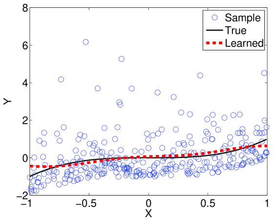
Figure 3: Illustrative example. The solid line denotes the true function, the circles denote samples, and the dashed line denotes the regressor obtained by LSIR.

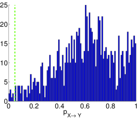
(a) Histogram of $p_{X\rightarrow Y}$ obtained by LSIR over $1000$ runs. The ground truth is to accept the null-hypothesis (thus the $p$-values should be large).

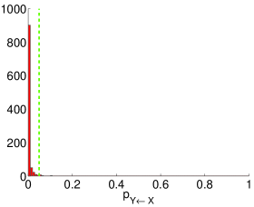
(b) Histograms of $p_{X\leftarrow Y}$ obtained by LSIR over $1000$ runs. The ground truth is to reject the null-hypothesis (thus the $p$-values should be small).

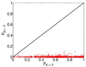
(c) Comparison of $p$-values for both directions ($p_{X\rightarrow Y}$ vs. $p_{X\leftarrow Y}$). Points below the diagonal line indicate successful trials.

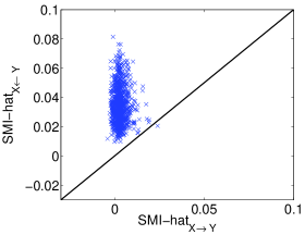
(d) Comparison of values of independence measures for both directions ($\widehat{\textnormal{SMI}}_{X\rightarrow Y}$ vs. $\widehat{\textnormal{SMI}}_{X\leftarrow Y}$). Points above the diagonal line indicate successful trials.

Figure 4: LSIR performance statistics in illustrative example.

Figure 3 depicts the regressor obtained by LSIR, giving a good approximation to the true function. We repeated the experiment $1000$ times with the random seed changed. For the significance level $5\%$, LSIR successfully accepted the null-hypothesis $992$ times out of $1000$ runs.

As Mooij et al. (2009) pointed out, beyond the fact that the $p$-values frequently exceed the pre-specified significance level, it is important to have a wide margin beyond the significance level in order to cope with, e.g., multiple variable cases. Figure 4(a) depicts the histogram of $p_{X\rightarrow Y}$ obtained by LSIR over $1000$ runs. The plot shows that LSIR tends to produce much larger $p$-values than the significance level; the mean and standard deviation of the $p$-values over $1000$ runs are $0.6114$ and $0.2327$, respectively.

Next, we consider the backward case where the roles of $X$ and $Y$ were swapped. In this case, the ground truth is that the input and the residual are dependent (see Figure 3). Therefore, the null-hypothesis should be rejected (i.e., the $p$-values should be small). Figure 4(b) shows the histogram of $p_{X\leftarrow Y}$ obtained by LSIR over $1000$ runs. LSIR rejected the null-hypothesis $989$ times out of $1000$ runs; the mean and standard deviation of the $p$-values over $1000$ runs are $0.0035$ and $0.0094$, respectively.

Figure 4(c) depicts the $p$-values for both directions in a trial-wise manner. The graph shows that LSIR perfectly estimates the correct causal direction (i.e., $p_{X\rightarrow Y}>p_{X\leftarrow Y}$), and the margin between $p_{X\rightarrow Y}$ and $p_{X\leftarrow Y}$ seems to be clear (i.e., most of the points are clearly below the diagonal line). This illustrates the usefulness of LSIR in causal direction inference.

Finally, we investigate the values of independence measure $\widehat{\textnormal{SMI}}$, which are plotted in Figure 4(d) again in a trial-wise manner. The graph implies that the values of $\widehat{\textnormal{SMI}}$ may be simply used for determining the causal direction, instead of the $p$-values. Indeed, the correct causal direction (i.e., $\widehat{\textnormal{SMI}}_{X\rightarrow Y}<\widehat{\textnormal{SMI}}_{X\leftarrow Y}$) can be found $999$ times out of $1000$ trials by this simplified method. This would be a practically useful heuristic since we can avoid performing the computationally intensive permutation test.

(a) dataset1

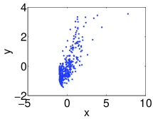
(b) dataset2

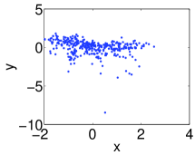
(c) dataset3

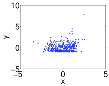
(d) dataset4

(e) dataset5

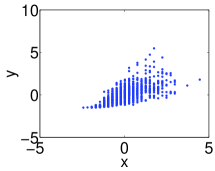
(f) dataset6

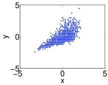
(g) dataset7

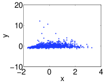
(h) dataset8

Figure 5: Datasets of the ‘Cause-Effect Pairs’ task in the NIPS 2008 Causality Competition (Mooij et al., 2008).

5.2 Benchmark Datasets

Next, we evaluate the performance of LSIR on the ‘Cause-Effect Pairs’ task in the NIPS 2008 Causality Competition (Mooij et al., 2008). The task contains $8$ datasets (see Figure 5), each has two statistically dependent random variables possessing inherent causal relationship. The goal is to identify the causal direction from the observational data. Since these datasets consist of real-world samples, our modeling assumption may be only approximately satisfied. Thus, identifying causal directions in these datasets would be highly challenging.

The $p$-values and the independence scores for each dataset and each direction are summarized in Table 1. The values of HSICR, which were also computed by the permutation test, were taken from (Mooij et al., 2009), but the $p$-values were rounded off to three decimal places to be consistent with the results of LSIR. When the $p$-values of both directions are less than $10^{-3}$, we concluded that the causal direction cannot be determined (indicated by ‘?’).

Table 1 shows that LSIR successfully found the correct causal direction for $7$ out of $8$ cases, while HSICR gave the correct decision only for $5$ out of $8$ cases. This implies that LSIR compares favorably with HSICR.

The values of independence measures described in Table 1 show that merely comparing the values of $\widehat{\textnormal{SMI}}$ is again sufficient for deciding the correct causal direction in LSIR (see the estimated causal directions described in the brackets). Actually, this heuristic also allows us to correctly identify the causal direction in Dataset 8. On the other hand, in HSICR, this convenient heuristic is not as useful as in the case of LSIR.

Table 1: Results for the ‘Cause-Effect Pairs’ task in the NIPS 2008 Causality Competition (Mooij et al., 2008). When the $p$-values of both directions are less than $10^{-3}$, we concluded that the causal direction cannot be determined (indicated by ‘?’). Estimated directions in the brackets are determined based on comparing the values of $\widehat{\textnormal{SMI}}$ or $\widehat{\textnormal{HSIC}}$.

(a) LSIR
Dataset $p$-values $\widehat{\textnormal{SMI}}$ Direction $X\rightarrow Y$ $X\leftarrow Y$ $X\rightarrow Y$ $X\leftarrow Y$ Estimated Truth 1 0.031 $<10^{-3}$ 0.0057 0.0265 $\rightarrow$ ($\rightarrow$) $\rightarrow$ 2 0.004 $<10^{-3}$ 0.0182 0.0301 $\rightarrow$ ($\rightarrow$) $\rightarrow$ 3 0.099 0.009 0.0090 0.0147 $\rightarrow$ ($\rightarrow$) $\rightarrow$ 4 0.102 0.173 0.0075 0.0051 $\leftarrow$ ($\leftarrow$) $\leftarrow$ 5 $<10^{-3}$ 0.012 0.0234 0.0108 $\leftarrow$ ($\leftarrow$) $\leftarrow$ 6 0.058 0.001 0.0079 0.0154 $\rightarrow$ ($\rightarrow$) $\rightarrow$ 7 0.009 0.018 0.0121 0.0110 $\leftarrow$ ($\leftarrow$) $\leftarrow$ 8 $<10^{-3}$ $<10^{-3}$ 0.0149 0.0244 ? ($\rightarrow$) $\rightarrow$
(b) HSICR
Dataset $p$-values $\widehat{\textnormal{HSIC}}$ Direction $X\rightarrow Y$ $X\leftarrow Y$ $X\rightarrow Y$ $X\leftarrow Y$ Estimated Truth 1 0.290 $<10^{-3}$ 0.0012 0.0060 $\rightarrow$ ($\rightarrow$) $\rightarrow$ 2 0.037 0.014 0.0020 0.0021 $\rightarrow$ ($\rightarrow$) $\rightarrow$ 3 0.045 0.003 0.0019 0.0026 $\rightarrow$ ($\rightarrow$) $\rightarrow$ 4 0.376 0.012 0.0011 0.0023 $\rightarrow$ ($\rightarrow$) $\leftarrow$ 5 $<10^{-3}$ 0.160 0.0028 0.0005 $\leftarrow$ ($\leftarrow$) $\leftarrow$ 6 $<10^{-3}$ $<10^{-3}$ 0.0032 0.0026 ? ($\leftarrow$) $\rightarrow$ 7 $<10^{-3}$ 0.272 0.0021 0.0005 $\leftarrow$ ($\leftarrow$) $\leftarrow$ 8 $<10^{-3}$ $<10^{-3}$ 0.0015 0.0017 $?$ ($\rightarrow$) $\rightarrow$

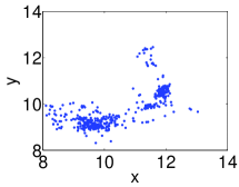
(a) lexA vs. uvrA

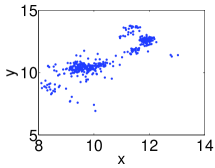
(b) lexA vs. recA

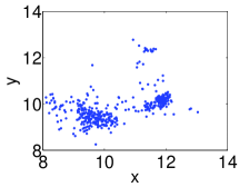
(c) lexA vs. uvrB

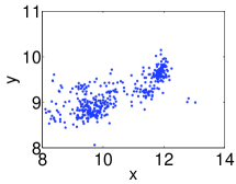
(d) lexA vs. uvrD

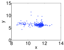
(e) crp vs. lacA

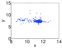
(f) crp vs. lacY

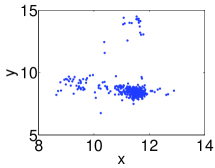
(g) crp vs. lacZ

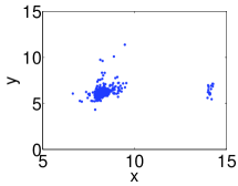
(h) lacI vs. lacA

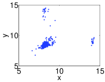
(i) lacI vs. lacZ

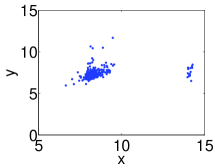
(j) lacI vs. lacY

Figure 6: Datasets of the E. coli task (Faith et al., 2007).

5.3 Gene Function Regulations

Finally, we apply our proposed LSIR method to the real-world biological datasets, which contain known causal relationships about gene function regulations from transcription factors to gene expressions.

Causal prediction is biologically and medically important because it gives us a clue for disease-causing genes or drug-target genes. Transcription factors regulate expression levels of their relating genes. In other words, when the expression level of transcription factor genes is high, genes regulated by the transcription factor become highly expressed or suppressed.

In this experiment, we select 10 well-known gene regulation relationships of E. coli (Faith et al., 2007), where each data contains expression levels of the genes over 445 different environments (i.e., 445 samples, see Figure 6)

The experimental results are summarized in Table 2, showing that LSIR successfully found the correct causal direction for $7$ out of $10$ cases, while HSICR gave the correct decision only for $4$ out of $10$ cases. Moreover, the causal direction can be efficiently chosen 9 out of 10 cases just by comparing the values of $\widehat{\textnormal{SMI}}$.

Table 2: Results for the ‘E. coli’ task. When the $p$-values of both directions are less than $10^{-3}$, we concluded that the causal direction cannot be determined (indicated by ‘?’). Estimated directions in the brackets are determined based on comparing the values of $\widehat{\textnormal{SMI}}$ or $\widehat{\textnormal{HSIC}}$.

(a) LSIR
Dataset $p$-values $\widehat{\textnormal{SMI}}$ Direction $X$ $Y$ $X\rightarrow Y$ $X\leftarrow Y$ $X\rightarrow Y$ $X\leftarrow Y$ Estimated Truth lexA uvrA $<10^{-3}$ $<10^{-3}$ 0.0177 0.0255 ? ($\rightarrow$) $\rightarrow$ lexA recA 0.024 0.061 0.0070 0.0053 $\leftarrow$ ($\leftarrow$) $\rightarrow$ lexA uvrB $<10^{-3}$ $<10^{-3}$ 0.0172 0.0356 ? ($\rightarrow$) $\rightarrow$ lexA uvrD 0.043 $<10^{-3}$ 0.0075 0.0227 $\rightarrow$ ($\rightarrow$) $\rightarrow$ crp lacA 0.143 $<10^{-3}$ -0.0004 0.0399 $\rightarrow$ ($\rightarrow$) $\rightarrow$ crp lacY 0.003 $<10^{-3}$ 0.0118 0.0247 $\rightarrow$ ($\rightarrow$) $\rightarrow$ crp lacZ 0.001 $<10^{-3}$ 0.0122 0.0307 $\rightarrow$ ($\rightarrow$) $\rightarrow$ lacI lacA 0.787 $<10^{-3}$ -0.0076 0.0184 $\rightarrow$ ($\rightarrow$) $\rightarrow$ lacI lacZ 0.002 $<10^{-3}$ 0.0096 0.0141 $\rightarrow$ ($\rightarrow$) $\rightarrow$ lacI lacY 0.746 $<10^{-3}$ -0.0082 0.0217 $\rightarrow$ ($\rightarrow$) $\rightarrow$
(b) HSICR
Dataset $p$-values $\widehat{\textnormal{HSIC}}$ Direction $X$ $Y$ $X\rightarrow Y$ $X\leftarrow Y$ $X\rightarrow Y$ $X\leftarrow Y$ Estimated Truth lexA uvrA $<10^{-3}$ $<10^{-3}$ 0.0865 0.1990 ? ($\rightarrow$) $\rightarrow$ lexA recA $<10^{-3}$ $<10^{-3}$ 0.2129 0.1625 ? ($\leftarrow$) $\rightarrow$ lexA uvrB 0.005 $<10^{-3}$ 0.0446 0.1335 $\rightarrow$ ($\rightarrow$) $\rightarrow$ lexA uvrD $<10^{-3}$ $<10^{-3}$ 0.0856 0.2427 ? ($\rightarrow$) $\rightarrow$ crp lacA 0.006 $<10^{-3}$ 0.0362 0.1162 $\rightarrow$ ($\rightarrow$) $\rightarrow$ crp lacY $<10^{-3}$ $<10^{-3}$ 0.0393 0.1303 ? ($\rightarrow$) $\rightarrow$ crp lacZ $<10^{-3}$ $<10^{-3}$ 0.0832 0.0836 ? ($\rightarrow$) $\rightarrow$ lacI lacA 0.004 $<10^{-3}$ 0.0368 0.1076 $\rightarrow$ ($\rightarrow$) $\rightarrow$ lacI lacZ $<10^{-3}$ $<10^{-3}$ 0.0666 0.1365 ? ($\rightarrow$) $\rightarrow$ lacI lacY 0.026 $<10^{-3}$ 0.0303 0.0927 $\rightarrow$ ($\rightarrow$) $\rightarrow$

6 Conclusions

In this paper, we proposed a new method of dependence minimization regression called least-squares independence regression (LSIR). LSIR adopts the squared-loss mutual information as an independence measure, and it is estimated by the method of least-squares mutual information (LSMI). Since LSMI provides an analytic-form solution, we can explicitly compute the gradient of the LSMI estimator with respect to regression parameters. A notable advantage of the proposed LSIR method over the state-of-the-art method of dependence minimization regression (Mooij et al., 2009) is that LSIR is equipped with a natural cross-validation procedure, allowing us to objectively optimize tuning parameters such as the kernel width and the regularization parameter in a data-dependent fashion. We experimentally showed that LSIR is promising in real-world causal direction inference.

References

- Aronszajn (1950) Aronszajn, N. (1950). Theory of reproducing kernels. Trans. the American Mathematical Society, 68, 337–404.
- Bishop (2006) Bishop, C. M. (2006). Pattern Recognition and Machine Learning. Springer, New York, NY.
- Cover and Thomas (2006) Cover, T. M. and Thomas, J. A. (2006). Elements of Information Theory. John Wiley & Sons, Inc., Hoboken, NJ, USA, 2nd edition.
- Efron and Tibshirani (1993) Efron, B. and Tibshirani, R. J. (1993). An Introduction to the Bootstrap. Chapman & Hall, New York, NY.
- Faith et al. (2007) Faith, J. J., Hayete, B., Thaden, J. T., Mogno, I., Wierzbowski, J., Cottarel, G., Kasif1, S., Collins, J. J., and Gardner, T. S. (2007). Large-scale mapping and validation of Escherichia coli transcriptional regulation from a compendium of expression profiles. PLoS Biology, 5(1), e8.
- Feuerverger (1993) Feuerverger, A. (1993). A consistent test for bivariate dependence. International Statistical Review, 61(3), 419–433.
- Fukumizu et al. (2009) Fukumizu, K., Bach, F. R., and Jordan, M. (2009). Kernel dimension reduction in regression. The Annals of Statistics, 37(4), 1871–1905.
- Geiger and Heckerman (1994) Geiger, D. and Heckerman, D. (1994). Learning Gaussian networks. In 10th Annual Conference on Uncertainty in Artificial Intelligence (UAI1994), pages 235–243.
- Gretton et al. (2005) Gretton, A., Bousquet, O., Smola, A., and Schölkopf, B. (2005). Measuring statistical dependence with Hilbert-Schmidt norms. In 16th International Conference on Algorithmic Learning Theory (ALT 2005), pages 63–78.
- Hoyer et al. (2009) Hoyer, P. O., Janzing, D., Mooij, J. M., Peters, J., and Schölkopf, B. (2009). Nonlinear causal discovery with additive noise models. In D. Koller, D. Schuurmans, Y. Bengio, and L. Botton, editors, Advances in Neural Information Processing Systems 21 (NIPS2008), pages 689–696, Cambridge, MA. MIT Press.
- Kanamori et al. (2009) Kanamori, T., Suzuki, T., and Sugiyama, M. (2009). Condition number analysis of kernel-based density ratio estimation. Technical report, arXiv. http://www.citebase.org/abstract?id=oai:arXiv.org:0912.2800.
- Kankainen (1995) Kankainen, A. (1995). Consistent Testing of Total Independence Based on the Empirical Characteristic Function. Ph.D. thesis, University of Jyväskylä, Jyväskylä, Finland.
- Kraskov et al. (2004) Kraskov, A., Stögbauer, H., and Grassberger, P. (2004). Estimating mutual information. Physical Review E, 69(066138).
- Kullback and Leibler (1951) Kullback, S. and Leibler, R. A. (1951). On information and sufficiency. Annals of Mathematical Statistics, 22, 79–86.
- Liu and Nocedal (1989) Liu, D. C. and Nocedal, J. (1989). On the limited memory method for large scale optimization. Mathematical Programming B, 45, 503–528.
- Mooij et al. (2008) Mooij, J., Janzing, D., and Schölkopf, B. (2008). Distinguishing between cause and effect. http:// www.kyb.tuebingen.mpg.de/bs/people/jorism/causality-data/.
- Mooij et al. (2009) Mooij, J., Janzing, D., Peters, J., and Schölkopf, B. (2009). Regression by dependence minimization and its application to causal inference in additive noise models. In 26th Annual International Conference on Machine Learning (ICML2009), pages 745–752, Montreal, Canada.
- Patriksson (1999) Patriksson, M. (1999). Nonlinear Programming and Variational Inequality Problems. Kluwer Academic, Dredrecht.
- Pearl (2000) Pearl, J. (2000). Causality: Models, Reasoning and Inference. Cambridge University Press, New York, NY, USA.
- Pearson (1900) Pearson, K. (1900). On the criterion that a given system of deviations from the probable in the case of a correlated system of variables is such that it can be reasonably supposed to have arisen from random sampling. Philosophical Magazine, 50, 157–175.
- Schölkopf and Smola (2002) Schölkopf, B. and Smola, A. J. (2002). Learning with Kernels. MIT Press, Cambridge, MA.
- Shimizu et al. (2006) Shimizu, S., Hoyer, P. O., Hyvärinen, A., and Kerminen, A. J. (2006). A linear non-Gaussian acyclic model for causal discovery. Journal of Machine Learning Research, 7, 2003–2030.
- Steinwart (2001) Steinwart, I. (2001). On the influence of the kernel on the consistency of support vector machines. Journal of Machine Learning Research, 2, 67–93.
- Suzuki and Sugiyama (2010) Suzuki, T. and Sugiyama, M. (2010). Sufficient dimension reduction via squared-loss mutual information estimation. In Proceedings of the Thirteenth International Conference on Artificial Intelligence and Statistics (AISTATS2010), volume 9 of JMLR Workshop and Conference Proceedings, pages 804–811.
- Suzuki et al. (2009) Suzuki, T., Sugiyama, M., Kanamori, T., and Sese, J. (2009). Mutual information estimation reveals global associations between stimuli and biological processes. BMC Bioinformatics, 10(S52).
- Vapnik (1998) Vapnik, V. N. (1998). Statistical Learning Theory. Wiley, New York, NY.