Formation of Rydberg macrodimers and their properties

Abstract

We investigate the interaction between two rubidium atoms in highly excited Rydberg states, and find that very long-range potential wells exist. These wells are shown to support many bound states. We calculate the properties of the wells and bound levels, and show that their lifetimes are limited by that of the constituent Rydberg atoms. We also show how these $\mu$m-size bound states can be populated via photoassociation (PA), and how the signature of the ad-mixing of various $\ell$-character producing the potential wells could be probed. We discuss how sharp variations of the PA rate could act as a switching mechanism with potential application to quantum information processing.

In recent years, the strong interactions between Rydberg atoms, due to their exaggerated properties Gallagher , have been detected experimentally Anderson ; Mourachko , and led to proposals for quantum computing Saffman-RMP , e.g. to achieve fast quantum gates jaksch00 ; grangier02 or to study quantum random walks cote-qrw . One effect of these interactions is the excitation blockade lukin01 , where a Rydberg atom prevents the excitation of nearby atoms tong04 ; singer04 ; Liebisch ; vogt06 ; Heidemann08 . Recently, dipole blockade between two atoms has been observed in microtraps grangier08 ; saffman09 , and a C-NOT gate implemented Saffman10 . Another signature of these strong interactions is the molecular resonance features in excitation spectra, first observed in Rb farooqi03 and in Cs atoms overstreet07 . Other molecular features involving Rydberg excitations, such as the so called trilobite and butterfly states, where one atom is in its ground state and another in a Rydberg state trilobites , have recently been detected pfau , while polyatomic molecules involving Rydberg electrons have also been studied Rost ; Sadeghpour .

In this article, we investigate the existence of long-range potential wells produced by two atoms excited into Rydberg states. As opposed to previous predictions of macrodimers macro-old – doubly-excited Rydberg molecules – with very shallow wells due to induced van der Waals (vdW) interactions, the macrodimers we study here are due to the strong mixing of $\ell$-characters of various Rydberg states. As we will see, these molecular wells are deeper (a few GHz), but still very extended with an equilibrium separation of 1 $\mu$m or so. We concentrate on wells existing in the vicinity of two rubidium (Rb) atoms excited to the $np$ Rydberg state, for which the relevant molecular symmetries are $0_{g}^{+}$, $0_{u}^{-}$, and $1_{u}$ Jovica .

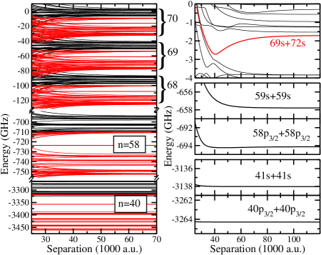
Figure 1: (Color online) $0^{+}_{g}$ molecular curves. Left panel: curves correlated to $n_{1}\ell_{1}+n_{2}\ell_{2}$ for $n\sim 70,69$, and 68 (top plot), 58 (middle) and 40 (bottom); black curves correspond to diagonalization near $np+np$ asymptotes, and red curves near $ns+ns$. Right panel: enlargements near the $70p_{3/2}+70p_{3/2}$ asymptote (top: with a well correlated to $69s+72s$), and the $R$ dependence of lower asymptotes (middle: $n\sim 58$; bottom: $n\sim 40$). Those last plots illustrate how the potential curves become flat as $n$ decreases.

We build our long-range molecular potential curves following the procedure described in Jovica ; we consider two free Rydberg atoms in states $|a\rangle\equiv|n,\ell,j,m_{j}\rangle$ and $|a^{\prime}\rangle\equiv|n^{\prime},\ell^{\prime},j^{\prime},m^{\prime}_{j}\rangle$, where $n$ is the principal quantum number, $\ell$ the orbital angular momentum, and $m_{j}$ is the projection of the total angular momentum $\vec{j}=\vec{\ell}+\vec{s}$ onto a quantization axis (chosen in the $z$-direction for convenience). The long-range molecular potential curves in Hund’s case (c) are calculated directly by diagonalizing the interaction Hamiltonian consisting of both the Rydberg-Rydberg interaction and the atomic fine structure Jovica . The basis states are built as follows:

$$|a,a^{\prime};\Omega_{g/u}\rangle\sim|a\rangle_{1}|a^{\prime}\rangle_{2}-p(-1)^{\ell+\ell^{\prime}}|a^{\prime}\rangle_{1}|a\rangle_{2}$$ (1)

where $\Omega=m_{j}+m^{\prime}_{j}$ is the projection of the total angular momentum on the molecular axis and is conserved. The quantum number $p$, describing the symmetry property under inversion, is 1(-1) for $g(u)$ states. For $\Omega=0$, the states’ symmetry under reflection must also be considered Jovica . The basis (1) assumes no overlap of charge distributions between the two atoms, so the long-range interaction can be expanded as an inverse power series of the nuclear separation distance $R$ Jovica .

Fig. 1 shows the results of the diagonalized interaction matrix for the $0_{g}^{+}$ symmetry near various $n\ell+n\ell$ asymptotes. The left panel shows curves for several states located around $np_{3/2}+np_{3/2}$ (in black) and $ns+ns$ (in red) near $n=70$, 69, 68, and lower asymptotes as well ($n\sim 58$ and $40$). These plots depict the strong mixing of different $\ell$-characters due mainly to the dipole-dipole interactions (although higher orders are also present). The right panel enlarges a major feature arising from the $\ell$-mixing near $70p_{3/2}+70p_{3/2}$, namely a large potential well (between 0 and -2.5 GHz) with a depth $D_{e}\sim 1$ GHz measured from its minimum (equilibrium separation) $R_{e}$ at roughly 40,500 $a_{0}$ ($a_{0}$: Bohr radius), i.e. over 2 $\mu$m. The $R$-dependence for lower asymptotes is also shown on the same panel; as $n$ decreases the potential curves become flatter (for same $R$ interval and energy scale). This is particularly true as $n$ reaches 40 or so.

The long-range well correlated to the $(n-1)s+(n+2)s$ asymptote is a general feature for this system; we depict a few cases in Fig. 2(a). The well depth $D_{e}$ and equilibrium separation $R_{e}$ scale roughly as $n^{-3}$ and $n^{2.5}$ (Fig. 2(b)), respectively, in good agreement with the $D_{e}\!\propto\!n^{-3}$ and $R_{e}\!\propto\!n^{7/3}$ scalings expected for a dominantly dipolar coupling between states. This last result can be obtained by keeping only the major $n$-dependence, so that the interaction matrix between two asymptotes has the form $n^{-3}{\hat{h}}_{0}\!+\!n^{4}R^{-3}{\hat{h}}_{1}\!$ where ${\hat{h}}_{0}$ and ${\hat{h}}_{1}$ contain the energy spacings between the asymptotes and the strengths of the dipole-dipole coupling, respectively. If we define $\rho\!\equiv\!n^{7}R^{-3}$ and rewrite the interaction matrix as $n^{-3}({\hat{h}}_{0}\!+\!\rho{\hat{h}}_{1})$, it becomes clear that its eigenvalues $E_{i}$ take the form $E_{i}\!=\!n^{-3}f_{i}(\rho)$. Since $\partial E_{i}/\partial R\!=\!-3n^{4}R^{-4}f^{\prime}_{i}(\rho)\!=\!0$ at an extremum, we must have $f^{\prime}_{i}(\rho)\!=\!0$, which is only fulfilled for some particular values $\rho_{e}$. In the parameter space of $R$ and $n$, this leads to $\rho_{e}\!=\!n^{7}R^{-3}|_{R_{e}}\!=\!{\rm const.}$ so that $R_{e}\!\propto\!n^{7/3}$, and $f_{i}(\rho_{e})\!=\!n^{3}E_{i}|_{D_{e}}\!=\!{\rm const.}$ so that $D_{e}\!\propto\!n^{-3}$. The difference between the analytical and numerical scalings reflects the more complex nature of the coupling than the assumed dipolar interaction.

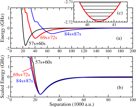
Figure 2: (Color online) $0^{+}_{g}$ wells correlated to the $(n-1)s+(n+2)s$ asymptote for $n=58$, 70 and 85: (a) un-scaled, and (b) scaled to $n=58$ with $D_{e}\sim n^{-3}$ and $R_{e}\sim n^{2.5}$. In (c), we show the deepest bound levels for $n=70$ (original scale).

We return to the curve correlated to the $69s+72s$ asymptote in the $0_{g}^{+}$ symmetry. Its well is deep enough to support several bound molecular levels, a few of which are listed in Table  1 and shown in Fig. 2(c). Since the levels are separated by a few MHz, they could be detected by spectroscopic means. Oscillation periods of a few $\mu$s, related to the MHz frequency of these deepest levels, are rapid enough to allow several oscillations during the lifetime of the Rydberg atoms (roughly a few 100 $\mu$s for $n\sim 70$). The classical inner and outer turning points of the levels indicate very extended molecules, hence we keep the term macrodimer to describe them.

The molecular electronic states $|\chi_{\lambda}(R)\rangle$ corresponding to the potential curves $U_{\lambda}(R)$ are composed of several molecular electronic basis states (1), the exact mixing (after diagonalization) varying with $R$:

$$|\chi_{\lambda}(R)\rangle=\sum_{j}c_{j}^{(\lambda)}(R)|j\rangle.$$ (2)

Here, $c_{j}^{(\lambda)}(R)$ are the eigenvectors and $|j\rangle$ the electronic basis states. As an example, we illustrate the composition of the well correlated to the $69s+72s$ asymptote in Fig. 3(a). If we write $|aa^{\prime}\rangle\equiv|a,a^{\prime};0_{g}^{+}\rangle$, this well is composed primarily of $|j\rangle=|69s72s\rangle$, $|70s71s\rangle$, $|70p_{3/2}70p_{1/2}\rangle$, $|69p_{3/2}71p_{1/2}\rangle$, and $|69p_{1/2}71p_{3/2}\rangle$; these states are indicated by different colors in Fig. 3(a). Using the same color labeling, we show the corresponding probabilities $|c_{j}(R)|^{2}$ of all five states against $R$ in Fig. 3(b). As expected, the right side of the well (near the $69s+72s$ asymptote) is composed primarily of the $|69s72s\rangle$ state, while the left side contains mostly $|69p_{1/2}71p_{3/2}\rangle$, a state whose asymptote is above $69s+72s$. Although one could have expected $|68p72p\rangle$ to provide most of the mixing, as suggested by Fig. 3(a), the proximity of the $69s+72s$ and $69p_{1/2}+71p_{3/2}$ asymptotes and their strong dipole coupling result in this larger mixing. The probability for $|68p_{3/2}72p_{1/2}\rangle$ is also included in Fig. 3(b).

Table 1: Energies of the deepest bound levels (from the bottom of the well) and classical turning points for the well correlated to the $69s+72s$ asymptote of the $0_{g}^{+}$ symmetry.

$v$	Energy (MHz)	$R_{1}$ (a.u.)	$R_{2}$ (a.u.)
0	0.831242	40,228	40,679
1	2.499032	40,068	40,849
2	4.166823	39,959	40,970
3	5.824596	39,870	41,068
4	7.477361	39,795	41,154
5	9.125118	39,728	41,233

The coupling to states correlated to lower asymptotes could lead to predissociation of the macrodimers and their decay into free atoms, heating up the sample with more energetic collisions and ionization. To estimate the predissociation lifetime of our bound states, and because of the large number of coupled electronic states, we assume that the total resonance width $\Gamma_{1}$ associated to the nonadiabatic transition from the molecular state 1 is just the sum over the widths $\Gamma_{1i}$ associated to transitions to individual adiabatic curves $i$, namely $\Gamma_{1}=\Sigma_{i}\,\Gamma_{1i}$. To compute the widths, we use a simple two-channel approach in which the nonadiabatic coupling $V_{1i}$ between the close channel corresponding to the molecular bound state (with electronic adiabatic basis state $|\chi_{1}(R)\rangle$), and the open channel corresponding to the dissociation state (with electronic adiabatic basis state $|\chi_{i}(R)\rangle$), is $V_{1i}(R)=-\frac{m_{e}}{\mu}\langle\chi_{1}(R)|\frac{\partial}{\partial R}|\chi_{i}(R)\rangle\frac{\partial}{\partial R}$, where $\mu$ is the reduced mass of the system. We then obtain the width $\Gamma_{1i}$ using a Green’s function method Friedrich : $\Gamma_{1i}=2\pi|\langle\phi_{v}|V_{1i}|\phi_{\rm reg}\rangle|^{2}$, where $\phi_{\rm reg}(R)$ is the regular, energy normalized solution of the open channel $i$ (in the absence of channel coupling), and the bound vibrational state $\phi_{v}(R)$ in the closed channel 1. For the 69$s$72$s$ $0_{g}^{+}$ potential curve, this approach give predissociation lifetimes that are extremely long, at least $10^{2}$ years, and we thus can conclude that these long-range Rydberg molecules are limited by the lifetimes of the Rydberg atoms themselves. This result could be expected, since the most important states contributing to the well are above the $69s+72s$ asymptote (Fig. 3(b)). We note however that for other wells due to mixing with lower asymptotic electronic electronic states, predissociation would play a major role in the lifetime of macrodimers.

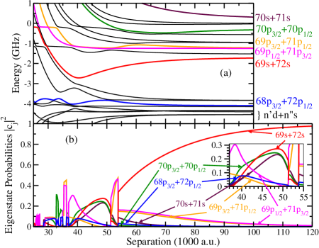
Figure 3: (Color Online) (a) Potential well correlated to the $69s+72s$ asymptote, and (b) its composition, with probabilities $|c_{j}(R)|^{2}$ of electronic basis $|j\rangle$ vs. $R$ (inset: zoom of the inner region). Same color code used in (a) and (b): see text.

In order to detect and probe the properties of the macrodimers predicted above, one can photoassociate two ground state atoms using intermediate Rydberg states that provide good overlap with the target long-range molecular states. Exciting the two ground state atoms into an intermediate Rydberg state $ns$, $np$, or $nd$ will allow us to probe the different $\ell$-characters (Fig. 3) in the bound level. The photoassociation (PA) rate ${\sf K}_{v}$ into a bound level $v$ can be calculated  Robin98 using

$${\sf K}_{v}\propto I_{1}I_{2}\left|\langle\phi_{v}|\langle\chi_{\lambda=1}|e^{2}r_{1}r_{2}|\chi_{g}\rangle|\phi_{g}\rangle\right|^{2},$$ (3)

where $I_{1}$ and $I_{2}$ are the intensities of laser 1 and 2, $|\phi_{v}(R)\rangle$ and $|\chi_{\lambda=1}(R)\rangle$ are the radial and electronic wave functions inside the well, respectively, $|\phi_{g}(R)\rangle$ and $|\chi_{g}(R)\rangle$ are the radial and electronic wave functions of the ground state, respectively, and $r_{i}$ and $e$ are the location and charge of the electron $i$. Using expression (2) for $|\chi_{\lambda=1}(R)\rangle$, and assuming that $|\chi_{g}\rangle$ is independent of $R$ (corresponding to a flat curve), we can rewrite (3) as

$${\sf K}_{v}\propto I_{1}I_{2}\sum_{j}\left|(d_{1}d_{2})_{j}\right|^{2}\left|\int_{0}^{\infty}\!\!\!\!dR\phi_{v}^{*}(R)c_{j}^{*}(R)\phi_{g}(R)\right|^{2},$$ (4)

where $d_{1}=\langle n_{j}\ell_{j}|er_{1}|n_{g}\ell_{g}\rangle$ and $d_{2}=\langle n^{\prime}_{j}\ell^{\prime}_{j}|er_{2}|n^{\prime}_{g}\ell^{\prime}_{g}\rangle$ are the electronic dipole moments between electronic states $|a_{g},a^{\prime}_{g}\rangle$ and $|a_{j},a^{\prime}_{j}\rangle$ for atom 1 and atom 2, respectively.

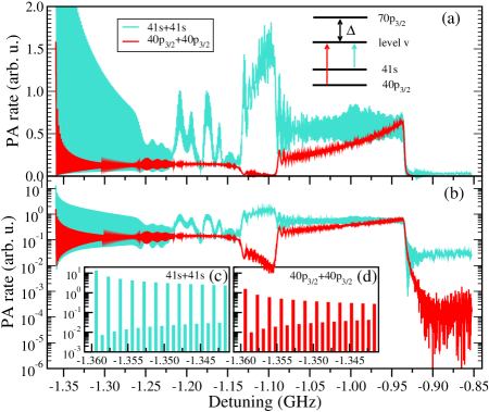
Figure 4: (Color online) PA rate vs. the detuning $\Delta$ from the $70p_{3/2}$ atomic state (a) on a linear scale, and (b) on a logarithmic scale. The intermediate state $|41s,41s\rangle$ populates the $|np,n^{\prime}p\rangle$ character in the well (turquoise), and the $|40p_{3/2},40p_{3/2}\rangle$ the $|ns,n^{\prime}s\rangle$ (red): (c) and (d) show the rate for the deepest levels (see text).

We calculate ${\sf K}_{v}$ by assuming that the Rb $5s$ atoms are first excited to an intermediate state that we consider to be the electronic “ground” states $|\chi_{g}\rangle$, before being excited to their final electronic states. For simplicity, we consider lower asymptotes in the vicinity of $n=40$ for which $|\chi_{g}\rangle$ does not vary with $R$ (Fig. 1). As shown in Fig. 3, the final electronic state contain mostly $|np,n^{\prime}p\rangle$ or $|ns,n^{\prime}s\rangle$; thus, we assume transitions from $40p_{3/2}+40p_{3/2}$ to the $ns+n^{\prime}s$ components and from $41s+41s$ to the $np+n^{\prime}p$ components. In Fig. 4, we show ${\sf K}_{v}$ against the detuning $\Delta$ from the atomic 70$p_{3/2}$ levels. For simplicity, we set $\phi_{g}(R)$ constant, although other choices could be made to enhance ${\sf K}_{v}$, such as a gaussian corresponding to the motion of atoms trapped in optical tweezers. The PA rate starting from both atoms in $40p_{3/2}$ is shown in red, and from $41s$ in turquoise, respectively, on a linear scale in (a) and a logarithmic scale in (b). In both cases, the rapid oscillation between a large rate for an even bound level ($v=0,2,4,\dots$) and a small rate for odd levels ($v=1,3,5,\dots$) gives the apparent envelop of the signal. This is illustrated in Figs. 4(c) and (d), where a zoom of the deepest levels $v$ is shown for both “ground” states (on a log-scale). This can be understood from the integral in Eq.(4), which is near zero for an odd wave function $\phi_{v}(R)$.

The signature of a macrodimer would manifest itself by the appearance of a signal starting at $\Delta\sim-0.93$ GHz red-detuned from the 70$p_{3/2}$ atomic level, and ending abruptly at $\sim-1.36$ GHz. In addition, the PA rate from either “ground” state $40p_{3/2}$ or $41s$ can reveal the details of the $\ell$-mixing in the potential well. First, the overall larger signal for $41s$ reflects the scaling of $d_{1}d_{2}$ appearing in Eq.(4), with $41s$ being closer than $40p_{3/2}$ to most atomic states appearing in the electronic molecular curve (see Fig. 3). As $\Delta$ increases from -1.36 GHz, ${\sf K}_{v}$ mimic the probabilities $|c_{j}(R)|^{2}$. For $41s$, the progressive decrease followed by sharp increases between $-1.22$ and $-1.16$ GHz correspond to the slow decreases of most $|np,n^{\prime}p\rangle$ components between $R\sim 40-50$ a.u. and their sharp increases around $R\sim 33-35$ a.u. (especially from $|69p_{1/2},71p_{3/2}\rangle$, $|69p_{3/2},71p_{1/2}\rangle$, and $|70p_{3/2},70p_{1/2}\rangle$; see Fig. 3). This is followed by another large feature between $-1.13$ and $-1.09$ GHz (corresponding to the sharp increase in $|69p_{1/2},71p_{3/2}\rangle$ and $|69p_{3/2},71p_{1/2}\rangle$ around $R\sim 53,000$ a.u.), and a “steady” rate before the signal drops to basically zero. For $40p_{3/2}$, we obtain two obvious features: first, a significant drop in ${\sf K}_{v}$ between $-1.13$ and $-1.09$ GHz which mirrors the decrease mainly in $|69s,72s\rangle$, and second, a steady growth corresponding to the rising probability of $|69s,72s\rangle$ beginning at about $55,000$ a.u. (before the signal drops to basically zero).

In conclusion, we have shown the existence of potential wells for the $0_{g}^{+}$ symmetry of doubly-excited atoms due to $\ell$-mixing. These wells support several bound levels separated by a few MHz with lifetimes limited by the Rydberg atoms themselves. These vibrational levels could be populated and detected by photoassociation. We showed that the signature of macrodimers would be the appearance of a signal beginning and ending abruptly, and that features in that signal could be used to probe the $\ell$-character of the potential well. The detection of such extended molecules with a lot of internal energy is in itself a goal, and would allow to study how macrodimers are perturbed by surrounding ground state atoms. In addition to interesting exotic chemistry (e.g., by an approaching Rydberg atom leading to a strong ultra-long van der Waals complex), the dependence of the PA rate on the exact $\ell$-mixing (Fig. 4) could potentially be used as a switch with application in quantum information (e.g., by turning on and off the blockade effect jaksch00 ).

The work of N.S. was supported by the National Science Foundation, and the work of R.C. in part by the Department of Energy, Office of Basic Energy Sciences.

References

- (1) T.F. Gallagher, Rydberg Atoms (Cambridge University Press, Cambridge, 1994).
- (2) W.R. Anderson, J.R. Veale, T.F. Gallagher, Phys. Rev. Lett. 80, 249 (1998).
- (3) I. Mourachko et al., Phys. Rev. Lett. 80, 253 (1998).
- (4) M. Saffman, T. G. Walker, and K. Mølmer, arXiv:0909.4777v3 (2010).
- (5) D. Jaksch et al., Phys. Rev. Lett. 85, 2208 (2000).
- (6) I.E. Protsenko, G. Reymond, N. Schlosser, and P. Grangier, Phys. Rev. A 65, 052301 (2002).
- (7) R. Côté, A. Russell, E. E. Eyler, and P. L. Gould, N. J. Phys., 8, 156 (2006).
- (8) M.D. Lukin et al., Phys. Rev. Lett. 87, 037901 (2001).
- (9) D. Tong et al. Phys. Rev. Lett. 93, 063001 (2004).
- (10) K. Singeret al.Phys. Rev. Lett. 93, 163001 (2004).
- (11) T. Vogt et al.Phys. Rev. Lett. 97, 083003 (2006).
- (12) T. C. Liebisch, A. Reinhard, P. R. Berman, and G. Raithel, G. Phys. Rev. Lett 95, 253002 (2005).
- (13) R. Heidemann et al.Phys. Rev. Lett. 100, 033601 (2008).
- (14) A. Gaëtan et al. Nature Phys. 5, 115 (2009).
- (15) E. Urban et al., Nature Phys. 5, 110 (2009).
- (16) L. Isenhower et al., Phys. Rev. Lett. 104, 010503 (2010).
- (17) S. M. Farooqi et al., Phys. Rev. Lett. 91, 183002 (2003).
- (18) K. R. Overstreet, A. Schwettmann, J. Tallant, and J. P. Shaffer, Phys. Rev. A 76, 011403 (2007).
- (19) C. H. Greene, A. S. Dickinson, and H. R. Sadeghpour, Phys. Rev. Lett. 85, 2458 (2000).
- (20) B. Vera et al., Nature 458, 1005 (2009).
- (21) I. C. H. Liu and J. M. Rost, Eur. Phys. J. D 40, 65 71 (2006); I. C. H. Liu, J. Stanojevic, and J. M. Rost, Phys. Rev. Lett 102, 173001 (2006); V. Bendkowsky et al., arXiv:0912.4058v1.
- (22) S. T. Rittenhouse and H. R. Sadeghpour, Phys. Rev. Lett. 104, 243002 (2010).
- (23) C. Boisseau, I. Simbotin, and R. Côté, Phys. Rev. Lett. 88, 133004 (2002).
- (24) J. Stanojevic et al., Eur. Phys. J. D 40, 3-12 (2006); J. Stanojevic et al., Phys. Rev. A 78, 052709 (2008).
- (25) H. Friedrich, Theoretical Atomic Physics, Second Edition, Springer-Verlag, 1998, ISBN 3540641246.
- (26) R. Côté and A. Dalgarno, Phys. Rev. A 58, 498 (1998).