Spin waves in the block checkerboard antiferromagnetic phase

Abstract

Motivated by the discovery of new family 122 iron-based superconductors, we present the theoretical results on the ground state phase diagram, spin wave and dynamic structure factor of the extended $J_{1}-J_{2}$ Heisenberg model. In the reasonable physical parameter region of $K_{2}Fe_{4}Se_{5}$ , we find the block checkerboard antiferromagnetic order phase is stable. There are two acoustic branches and six optical branches spin wave in the block checkerboard antiferromagnetic phase, which has analytic expression in the high symmetry points. To compare the further neutron scattering experiments, we discuss the saddlepoint structure in the magnetic excitation spectrum and calculate the predicted inelastic neutron scattering pattern based on linear spin wave theory.

I Introduction

Searching high-$T_{c}$ superconductivity has been one of the central topics in condensed matter physicsLee-P-A-1 . Following the discovery of the copper-based superconductors two decades agoBednorz-1 , the second class of high-transition temperature superconductors has been reported in iron-based materialsKamihara-1 ; Chen-G-F-1 ; Lei-H-1 . The iron pnictides contains four typical crystal structures, such as 1111-type ReFeAsO (Re represents rare earth elements)Kondo-1 , 122 type Ba(Ca)Fe₂As₂Wray-1 ; Xu-Gang-1 , 111 type LiFeAsBorisenko-1 and 11 type FeSeKhasanov-1 . The parent compounds with all structures except the 11 type have the stripe like antiferromagnetic state as the ground state. By substituting a few percent of O with F Kondo-1 or Ba with KWray-1 ; Xu-Gang-1 , the compounds enter the superconducting (SC) phase from the SDW phase below $T_{c}$ . In addition to the above four crystal structures, a new family of iron-based superconducting materials with 122 type crystal structure have recently been discovered with the transition temperature $T_{c}$ as high as 33 K Guo-2 . However, these new ”122” compounds differ from the iron superconductors with the other structures in many aspectsMaziopa-1 . Firstly, the parent compound of the new ”122” material is proposed to be $K_{0.8}Fe_{1.6}Se_{2}$ with intrinsic $root5byroot5Fe$ vacancy ordering determined by various experimentsWei-Bao-1 ; Wei-Bao-2 ; Wei-Bao-3 . Secondly, the ground state for $K_{0.8}Fe_{1.6}Se_{2}$ is Mott insulator with block antiferromagnetic order, which is observed by the neutron diffraction experimentsWei-Bao-1 ; Wei-Bao-2 ; Wei-Bao-3 . By the first principles calculation, Yan et. alY-Z-Lu-1 and Cao et. alDai-J-H also found the block antiferromagnetic order is the most stable ground state for $K_{0.8}Fe_{1.6}As_{2}$.

To date, a number of researches have been carried out to study the nature of superconductivity and magnetic properties of these materials. The neutron scattering experiments by Bao et.alWei-Bao-3 have found the ground state of $K_{0.8}Fe_{1.6}As_{2}$ to be block anti-ferromagnetic with magnetic moment around $3.4\mu_{B}$. It has been proposed by several authors that the magnetic and superconducting instabilities are strongly coupled together and the properties of magnetic excitations, such as spin wave, play very crucial roles for the superconductivity in this family materials. Zhang et. alZhang-G-M-1 even suggested that the superconducting pairing may be mediated by coherent spin wave excitations in these materials.

In order to give the qualitative insight into the magnetic excitation properties in this system, we studied the spin wave spectrum using the Heisenberg model on the 2D square lattice with $\sqrt{5}\times\sqrt{5}$ vacancy pattern. There are four independent parameters are used in the model, which correspond to the nearest neighbor and next nearest neighbor coupling between spins. We first obtain the ground state phase diagram as the function of those parameters, based on which we calculate the spin wave spectrum as well as the spin dynamic structure factor using the Holstein-Primakov transformation. Our results demonstrate that the block checkerboard antiferromagnetic order is stable in a wide range of phase regime and there are two acoustic branches as well as six optical branches spin wave in this system, which can be measured by the future neutron scattering experiments.

II Model and Method

The simplest model that captures the essential physics in Fe-vacancies ordered material $K_{2}Fe_{4}Se_{5}$ can be described by the extended $J_{1}-J_{2}$ Heisenberg model on a quasi-two-dimensional lattice Dai-J-H ; Y-Z-Lu-1 ,

$$H = J_{1}\sum_{i,\delta,\delta^{\prime}(>\delta)}\overrightarrow{S}_{i,\delta}\cdot\overrightarrow{S}_{i,\delta^{\prime}}$$ (1)

$$+J^{\prime}_{1}\sum_{i,\gamma,\delta,\delta^{\prime}}\overrightarrow{S}_{i,\delta}\cdot\overrightarrow{S}_{i+\gamma,\delta^{\prime}}$$

$$+J_{2}\sum_{i,\delta,\delta^{\prime\prime}(>\delta)}\overrightarrow{S}_{i,\delta}\cdot\overrightarrow{S}_{i,\delta^{\prime\prime}}$$

$$+J^{\prime}_{2}\sum_{i,\gamma,\delta,\delta^{\prime\prime}}\overrightarrow{S}_{i,\delta}\cdot\overrightarrow{S}_{i+\gamma,\delta^{\prime\prime}}$$

Here, $\delta=1,2,3,4$ and $\gamma=1,2,3,4$; the first and second terms represent nearest-neighbor (n.n.) spin interactions in the intra- and inter- block, respectively, as shown in Fig.1. The third and forth term are second-neighbor ( n.n.n.) spin interactions which are taken to be independent on the direction in the intra- and inter- block. Here, i is the block index, $\gamma$ denotes the nearest-neighbor block of i block. $\delta^{\prime}$($\delta^{\prime\prime}$) represents the site-index which is n.n (n.n.n) site of site $\delta$. $J_{1}$ and $J^{\prime}_{1}$ ($J_{2}$ and $J^{\prime}_{2}$ ) indicate n.n. ( n.n.n.) couplings of intra- and inter-block, respectively, which are illustrated in Fig. 1. Here, we define $J_{2}$ is the energy unit.

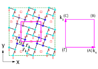
Figure 1: (color online)Schematic diagram of the 2 dimensional crystal and magnetic structure (single layer for $K_{2}Fe_{4}Se_{5}$ ) and the corresponding Brillouin Zone. On the left is the crystal structure and spin pattern of the pnictides $K_{2}Fe_{4}Se_{5}$ . The up-arrow(blue) and down-arrow(azure) atoms indicate the Fe-atoms with positive/negative magnetic moment, respectively. Here we show the considered model with nearest neighbor coupling $J_{1},J_{1}^{\prime}$ and next nearest neighbor coupling $J_{2},J_{2}^{\prime}$. The coupling within each block is $J(J_{1},J_{2})$, and the coupling between blocks is $J^{\prime}(J_{1}^{\prime},J_{2}^{\prime})$. On the right is the positive quadrant of the square-lattice Brillouin Zone showing wave-vectors $\Gamma=(0,0)$, $A=(\frac{2\pi}{\sqrt{10}a},0)$, $B=(\frac{2\pi}{\sqrt{10}a},\frac{2\pi}{\sqrt{10}a})$, $C=(0,\frac{2\pi}{\sqrt{10}a})$. With the high symmetry line, the spin wave are contained along the direction $\Gamma-A-B-\Gamma-C-B$. The purple solid line marks the magnetic unit cell. The iron vacancy site Fe is marked by the open square, and the occupied site Fe is marked by solid circle with the blue or reseda color indicating spin up or spin down.

In order to understand this $J_{1}-J_{2}$ Heisengerg Hamiltonian, we depict the typical block spin ground state and the 2D Brillouin zone (BZ) in Fig.1. The q-vectors used for defining the high symmetry line of the spin wave is also depicted. Each magnetic unit cell contains eight Fe atoms and two Fe vacancy which are marked by the open squares, as shown in Fig.1. The block checkerboard antiferromagnetic order are recently observed by the neutron diffraction experiment in the $K_{2}Fe_{4}Se_{5}$ material. An convenient way to understand the antiferromagnetic structure of $K_{2}Fe_{4}Se_{5}$ is to consider the four parallel magnetic moments in one block as a supermoment; and the supermoments then form a simple chess-board nearest-neighbor antiferromagnetic order on a square lattice, as seen from Fig.1a. The distance between the nearest-neighbor iron is defined as $a$. Then, the crystal lattice constant for the magnetic unit cell is $\sqrt{10}a$. Fig.1b is the 2D BZ for the magnetic unit cell.

We use Holstein-Primakoff (HP) bosons to investigate the spin wave of the block checkerboard antiferromagnetic ground state. As we know, linearized spin wave theory is a standard procedure to calculate the spin wave excitation spectrum and the zero-temperature dynamical structure factorAuerbach-1 ; D-X-Yao-1 . Firstly, we use HP bosons to replace the spin operators, as shown in Appendix A.

Using Holstein-Primakoff transformations, we can obtain the HP boson Hamiltonian,

$$H = \sum_{k}\psi_{k}^{\dagger}\mathcal{H}_{k}\psi_{k}+E_{0}-N\cdot E_{\left(k=0\right)}$$ (2)

Here, $\begin{smallmatrix}\psi_{k}^{\dagger}&=\end{smallmatrix}$ $\bigl{(}\begin{smallmatrix}a_{k1}^{\dagger}&a_{k2}^{\dagger}&a_{k3}^{\dagger}&a_{k4}^{\dagger}&b_{-k-1}&b_{-k-2}&b_{-k-3}&b_{-k-4}\end{smallmatrix}\bigr{)}$; $E_{0}$ is the classical ground state energy for block checkerboard antiferromagnetic order, $E_{0}=8J_{1}NS^{2}-4J^{\prime}_{1}NS^{2}+4J_{2}NS^{2}-8J^{\prime}_{2}NS^{2}$. The Specific expression for $\mathcal{H}_{k}$ is shown in Appendix B.

In the real space, we define the ’molecular orbital’ , which is the combination of HP boson operators in one block.

$$\begin{smallmatrix}\alpha_{i1}&=&\frac{1}{\sqrt{4}}\left(a_{i1}-a_{i2}+a_{i3}-a_{i4}\right)\\ \alpha_{i2}&=&\frac{1}{\sqrt{4}}\left(a_{i1}+a_{i2}-a_{i3}-a_{i4}\right)\\ \alpha_{i3}&=&\frac{1}{\sqrt{4}}\left(a_{i1}-a_{i2}-a_{i3}+a_{i4}\right)\\ \alpha_{i4}&=&\frac{1}{\sqrt{4}}\left(a_{i1}+a_{i2}+a_{i3}+a_{i4}\right)\\ \beta_{i-1}&=&\frac{1}{\sqrt{4}}\left(b_{i-1}-b_{i-2}+b_{i-3}-b_{i-4}\right)\\ \beta_{i-2}&=&\frac{1}{\sqrt{4}}\left(b_{i-1}+b_{i-2}-b_{i-3}-b_{i-4}\right)\\ \beta_{i-3}&=&\frac{1}{\sqrt{4}}\left(b_{i-1}-b_{i-2}-b_{i-3}+b_{i-4}\right)\\ \beta_{i-4}&=&\frac{1}{\sqrt{4}}\left(b_{i-1}+b_{i-2}+b_{i-3}+b_{i-4}\right)\end{smallmatrix}$$

Here, the $-$ represents the spin down block. The corresponding physical picture for each ’molecular orbital’ is shown in the Fig. 2.

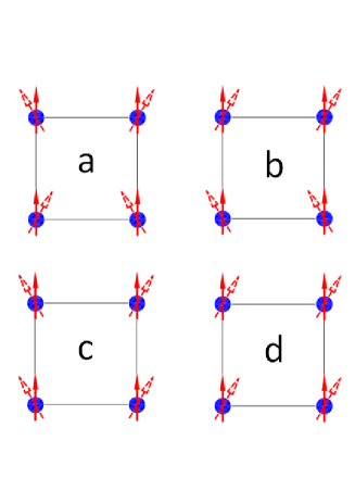
Figure 2: (color online) The schematic diagram for the ’molecular orbital’ in the $\Gamma$ point: (a) The deviation of spin in site 1 and 3 has the same phase for the corresponding wave function; and the deviation of spin in site 2 and 4 has the same phase for the corresponding wave function. But the different between the phase of wave function for site 1 and 2 is 180 degrees. (b)The deviation of spin in site 1 and 2 has the same phase for the corresponding the wave function; and the deviation of spin in site 3 and 4 has the same phase for the corresponding wave function. But the different between the phase of wave function for site 1 and 3 is 180 degrees. (c) The deviation of spin in site 1 and 4 has the same phase for the corresponding wave function; and the deviation of spin in site 2 and 3 has the same phase for the corresponding wave function. But the different between the phase of wave function for site 1 and 2 is 180 degrees. (d) The deviation of spin in site 1, 2, 3 and 4 all has the same phase for the corresponding wave function.

In the ’molecular orbital’ basis, the Hamiltonian becomes,

$$H_{k} = \sum_{k}\psi_{k}^{o\dagger}\mathcal{H}^{orbital}_{k}\psi_{k}^{o}$$ (3)

Here, $\begin{smallmatrix}\psi_{k}^{o\dagger}&=\end{smallmatrix}$ $\bigl{(}\begin{smallmatrix}\alpha_{k1}^{\dagger}&\alpha_{k2}^{\dagger}&\alpha_{k3}^{\dagger}&\alpha_{k4}^{\dagger}&\beta_{-k-1}&\beta_{-k-2}&\beta_{-k-3}&\beta_{-k-4}\end{smallmatrix}\bigr{)}$. The matrix elements for different ’molecular orbital’ in the same block is zero, which is interesting; and we discuss the Hamiltonian later. The Specific expression for $\mathcal{H}^{orbital}_{k}$ is shown in Appendix B.

Because the boson Hamiltonian are big, one must use numerical diagonalization to solve eigenvalues for spin wave, which has a standard procedureM-W-Xiao ; M-W-Xiao-1 ; M-W-Xiao-3 ; M-W-Xiao-4 ; M-W-Xiao-5 , as shown in Appendix C.

To further understand the physical properties in this spin system, we obtain the analytical eigenvalues and eigenvectors in some special k points, such as $k=(0,0)$ and $k=(\frac{\pi}{\sqrt{10}a},\frac{\pi}{\sqrt{10}a})$ point. In the $\Gamma$ point, the ’molecular orbital’ Hamiltonian becomes four $2\times 2$ block matrix $\bigl{(}\begin{smallmatrix}h_{m}&h_{m,m+4}\\ h_{m,m+4}&h_{m}\end{smallmatrix}\bigr{)}$ about $\alpha_{m}$ and $\beta_{-k-m}^{\dagger}$ ($m=1,2,3,4$), which indicates that the ’molecular orbital’ are intrinsic vibration modes for $\Gamma$ point. The spin waves at $\Gamma$ point are collective excitations of the same ’molecular orbital’ between different blocks.

From the $2\times 2$ block Hamiltonian, we obtain the eigenvalues in the $\Gamma$ point,

$$\begin{smallmatrix}\omega_{1}^{(0,0)}&=&S\sqrt{(4J_{1}-J^{\prime}_{1}-2J^{\prime}_{2})^{2}-(J^{\prime}_{1}-2J^{\prime}_{2})^{2}}\\ \omega_{2}^{(0,0)}=\omega_{3}^{(0,0)}&=&2S\sqrt{(J_{1}+J_{2}-J^{\prime}_{2})(J_{1}-J^{\prime}_{1}+J_{2}-J^{\prime}_{2})}\\ \omega_{4}^{(0,0)}&=&0\end{smallmatrix}$$

There are four Eigenvalues. The first eigenvalue is twofold degenerate, and its eigenvector is a combination by the first ’molecular orbital’ in the spin up and spin down block site, as shown in Fig.2a. The second and third eigenvalues are degenerate and each of them is twofold degenerate. Their eigenvector are combination by the second and third ’molecular orbital’ in the spin up and spin down block site, as shown in Fig.2b and Fig.2c, respectively. They are all optical branches due to the gap in the $\Gamma$ point. The final eigenvalue is also twofold degenerate. However, different from the above optical branches, it is a acoustic branch and always zero in $\Gamma$ point, which is imposed by Goldstone’s theorem.

As shown above, we can also discuss the physical properties in the $k=(\frac{\pi}{\sqrt{10}a},\frac{\pi}{\sqrt{10}a})$ point. From the boson Hamiltonian, we can obtain the eigenvalues in the $k=(\frac{\pi}{\sqrt{10}a},\frac{\pi}{\sqrt{10}a})$ point,

$$\begin{smallmatrix}\omega_{1}^{(\pi,\pi)}&=&-2SJ_{1}+S\sqrt{(2J_{1}-J^{\prime}_{1}-2J^{\prime}_{2})^{2}-{J^{\prime}_{1}}^{2}}\\ \omega_{2}^{(\pi,\pi)}&=&2SJ_{1}+S\sqrt{(2J_{1}-J^{\prime}_{1}-2J^{\prime}_{2})^{2}-{J^{\prime}_{1}}^{2}}\\ \omega_{3}^{(\pi,\pi)}=\omega_{4}^{(\pi,\pi)}&=&S\sqrt{(2J_{1}-J^{\prime}_{1}+2J_{2}-2J^{\prime}_{2})^{2}-4{J^{\prime}_{2}}^{2}-{J^{\prime}_{1}}^{2}}\\ \end{smallmatrix}$$

There are also four Eigenvalues and each of them are twofold degenerate. Six eigenvalue are optical branches and two eigenvalue are acoustic branches. The third and forth eigenvalue are always degenerate in $k=(\frac{\pi}{\sqrt{10}a},\frac{\pi}{\sqrt{10}a})$ point.

Now, we have five different eigenvalues for spin wave in the special point, which can be used to fit the experimental data in order to get the n.n. ( n.n.n.) couplings of intra- and inter-block, $J_{1}$ , $J^{\prime}_{1}$ ($J_{2}$ , $J^{\prime}_{2}$ ) . Then using this interaction parameters, we can obtain the spin wave along all the BZ by numerical diagonalization method.

III RESULTS AND DISCUSSION

In this section, we first present the phase diagram of the $J_{1}-J_{2}$ model. Then we discuss the spin wave and spin dynamical factor in the block stipe antiferromagnetic phase.

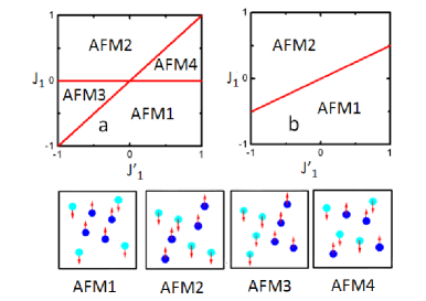
Figure 3: (color online) The phase diagram for the $J_{1}(J_{1}^{\prime})-J_{2}(J_{2}^{\prime})$ model. The phases are defined in Ref. 17, among which the AFM1 phase is the block checkerboard antiferromagnetic phase observed in the neutron diffraction experiment. The blue/azure atoms indicate the Fe-atoms with positive/negative magnetic moment, respectively. The magnetic configuration for AFM2, AFM3 and AFM4 is shown. (a) The phase diagram for the interaction parameter $J_{2}=1,J_{2}^{\prime}=J_{2}$. (b) The phase diagram for the interaction parameter $J_{2}=1,J_{2}^{\prime}=2.5J_{2}$.

To investigate the phase diagram for the $J_{1}-J_{2}$ Heisenberg model, we use the stochastic Monte Carlo(MC) method to investigate the system ground state. In the reasonable physical parameter region, the phase diagram for the $J_{1}-J_{2}$ Heisenberg model is given in Fig.3, which is plotted in the plane $J_{1}/J_{2}-J_{1}^{\prime}/J_{2}$ at fixed value $J_{2}^{\prime}/J_{2}$. We obtain four stable phases in the case $J_{2}^{\prime}/J_{2}=1$. The first one is the block checkerboard antiferromagnetic order phase, denoted by AFM1 in Fig.1, which has been observed by the experimentWei-Bao-1 ; Wei-Bao-2 . This phase is our interested in the study of iron-based superconductors. Obviously, when the coupling $J_{1}$ is negative, the spin favors to form ferromagnetic configuration in the blocks. simultaneously, when the coupling $J_{1}^{\prime}$ is positive, the spin favors to form anti-ferromagnetic configuration between the nearest-neighbor block. Of course, when $J_{1}^{\prime}$ is negative, but small, the interaction $J_{1}$ and $J_{2}^{\prime}$ are dominant and the block checkerboard antiferromagnetic phase is also stable in this region. In the case $J_{2}^{\prime}/J_{2}=1$, the block checkerboard antiferromagnetic phase stably exists when the following conditions are satisfied: $J_{1}<0$ and $J_{1}^{\prime}>J_{1}$ . In the parameter region $J_{1}>0$ and $J_{1}>J_{1}^{\prime}$ , the system favors to stay in the AFM2 phase, as seen in the Fig. 3(a). In this phase, the antiferromagnetic order in the block arises from the antiferromagnetic coupling $J_{1}$. On the other hand, the spin system favors the AFM3 phase when $J_{1}^{\prime}<J_{1}<0$ , which is mainly attributed to the dominant interaction $J_{1}^{\prime}$ in this parameter regions. Similar to the phase AFM3, the system stay in the AFM4 phase in the region $0<J_{1}<J_{1}^{\prime}$, as seen in the Fig. 3(a). To concretely investigate the spin properties in this system and compare the theory calculation with experimental results, in what follows, we change the parameter value $J_{2}^{\prime}/J_{2}=1$ to $J_{2}^{\prime}/J_{2}=2.5$ to investigate the phase diagram. In this parameter region, the antiferromagnetic coupling $J_{2}^{\prime}$ is dominant. Different from the first case, there are only two phase, AFM1 and AFM2, in the phase diagram. The two phase is separated by the line $J_{1}=0.5J_{1}^{\prime}$. Below the line, the phase is AFM1 phase, otherwise, the phase is AFM2 phase. It is interesting to ask in which region the realistic parameters of the iron pnictides fall. From the LDA calculations, Cao et al suggested that $J_{1}=-29$ mev, $J_{1}^{\prime}=10$ mev, $J_{2}=39$ mev and $J_{2}^{\prime}=95$ mevDai-J-H . Such a set of parameters falls in the block checkerboard antiferromagnetic phase in Fig.3(a) and (b), implying that the $K_{2}Fe_{4}Se_{5}$ should have the block checkerboard antiferromagnetic order. This fact tells us we only need to focus on parameter region in the AFM1 phase.

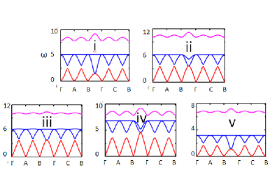
Figure 4: (color online)Acoustic and optical spin-wave branches for linear spin-wave theory, T = 0, as a function of k along selected high symmetry directions in the magnetic unit cell Brillouin Zone. (i)$J_{1}=-1$, $J_{1}^{\prime}=0.2$, $J_{2}=1$ and $J_{2}^{\prime}=2.5$, (ii)$J_{1}=-1.5$, $J_{1}^{\prime}=0.2$, $J_{2}=1$ and $J_{2}^{\prime}=2.5$. , (iii) $J_{1}=-1$, $J_{1}^{\prime}=1.5$, $J_{2}=1$ and $J_{2}^{\prime}=2.5$. , (iv) $J_{1}=-1$, $J_{1}^{\prime}=0.2$, $J_{2}=0.2$ and $J_{2}^{\prime}=2.5$. , (v) $J_{1}=-1$, $J_{1}^{\prime}=0.2$, $J_{2}=1$ and $J_{2}^{\prime}=1.5$. The x-axis correspond to the k point along the selected direction in Fig.1b. y-axis correspond to the energy for spin wave; the energy unit is $J_{2}=1$ except case (iv).

First of all, we use numerical diagonalization method to investigate the spin wave dispersion relations along the high symmetry direction in different situations. In the numerical calculation, it is convenient to set $J_{2}=1$; and comparing with experiments, the actual energy scale of $J_{2}$ for the specifical material can be deduced. Motivated by the first principle reported parametersDai-J-H , we first study the set of parameter: (i)$J_{1}=-1$, $J_{1}^{\prime}=0.2$, $J_{2}=1$ and $J_{2}^{\prime}=2.5$. However, to study the influence of interaction parameters on the spin-wave spectra, we also investigate four different sets of parameter: (ii)$J_{1}=-1.5$, $J_{1}^{\prime}=0.2$, $J_{2}=1$ and $J_{2}^{\prime}=2.5$. , (iii) $J_{1}=-1$, $J_{1}^{\prime}=1.5$, $J_{2}=1$ and $J_{2}^{\prime}=2.5$. , (iv) $J_{1}=-1$, $J_{1}^{\prime}=0.2$, $J_{2}=0.2$ and $J_{2}^{\prime}=2.5$. , (v) $J_{1}=-1$, $J_{1}^{\prime}=0.2$, $J_{2}=1$ and $J_{2}^{\prime}=1.5$. In Fig. 4, we plot spin wave dispersions along high-symmetry direction $\Gamma-A-B-\Gamma-C-B$ in the BZ for different interaction parameters. In all cases, there are one acoustic and three optical spin-wave branches(each of them is twofold degenerate). For the acoustic branches, the gap of spin wave in $\Gamma$ point is always zero due to Goldstone’s theorem. In the first case, the vibration mode for acoustic branches is shown in Fig.2(d). It is the collective excitation mode for the forth ’molecular orbital’ in one block with the forth ’molecular orbital’ in other blocks. And the relative phase in a ’molecular orbital’ is only depend on the momentum $k$ and independent on the interaction parameters. However, the relative phase between different block’s ’molecular orbital’ is dependent on the specific interaction parameters. The optical gap in the $\Gamma$ point is dependent on the specific interaction parameters by contraries. As discussed in Eq.II, two of the three optical branches are degenerate at $\Gamma$ point. Away from $\Gamma$ point, the two degenerate optical branches split. For example, with the increasing of k along the $\Gamma B$ direction, the optical branch for the second ’molecular orbital’ (Fig. 2b) is almost no change. In contrast, the optical branch for the vibration mode of third ’molecular orbital’(Fig.2c) has obvious dispersion, which can be clearly seen in Fig.4a. The reason that causes the splitting of spin wave can be attributed that the vibration mode of different ’molecular orbital’ is not isotropic and dependent on the momentum $k$. Therefore, different vibration mode has different behavior in different momentum direction. Similar to the the above two optical branches, the third optical branch is related to the vibration mode of the first ’molecular orbital’, which is a independent branch.

With the change of interaction parameters, we can investigate the influence of the interaction parameters on the spin wave, as shown in Fig.4. Firstly, in all cases, the acoustic branches is always zero in $\Gamma$ point and there are always twofold degenerate in $\Gamma$ and $k=(\frac{\pi}{\sqrt{10}a},\frac{\pi}{\sqrt{10}a})$ point. In the following, we compare the spin wave dispersion relation by the change of interaction parameters. Comparing with the Fig.4 (i) and Fig.4 (ii), we find that with the increasing of $J_{1}$, the spin wave dispersions become bigger in different k point, especially for the acoustic branch in the $k=(\frac{\pi}{\sqrt{10}a},\frac{\pi}{\sqrt{10}a})$ point. From the Fig.4 (i) and Fig.4 (iii), we observe that the amplitude of the second optical branch becomes large with the increasing of $J^{\prime}_{1}$. It also change the energy for spin wave in different k point, especially in the $k=(\frac{\pi}{\sqrt{10}a},\frac{\pi}{\sqrt{10}a})$ point. With the increasing of $J^{\prime}_{1}$, the amplitude of the second optical branch becomes more and more clear. With comparing the Fig.4(i) and Fig.4 (iv), we observe that the interval for the first and second optical branch becomes smaller with the increasing of $J_{2}$. The energy for spin wave is also changed in different k point, especially in the $k=(\frac{\pi}{\sqrt{10}a},\frac{\pi}{\sqrt{10}a})$ point. Like all the above cases, the spin wave dispersion also has some change in the intensity with the increasing of $J^{\prime}_{2}$. However, the interval for the first and second optical branch becomes larger, which is one of the most obvious features for increasing $J^{\prime}_{2}$, as seen in Fig.4(i) and Fig.4 (v).

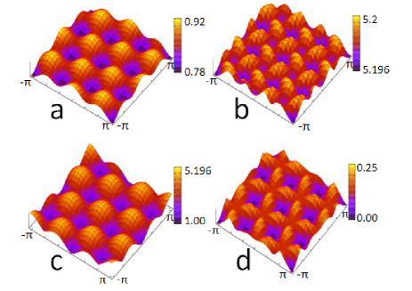
Figure 5: (color online) 3D spin wave dispersion for the parameter set of $J_{1}=-1$, $J_{1}^{\prime}=0.2$, $J_{2}=1$ and $J_{2}^{\prime}=2.5$ in the extended BZ for one block, as seen in Fig.1 a. The energy is in units of $J_{2}$. (a) spin wave dispersion for first optical branch. (b) spin wave dispersion for second optical branch. (c) spin wave dispersion for third optical branch. (d) spin wave dispersion for Acoustic branch. The x-axis and y-axis correspond to $3k_{x}-k_{y}$ and $k_{x}+3k_{y}$ direction respectively.

Fig.5 shows the typical 3 dimension spin wave spectrum in the extended BZ for one block of the first set of parameters in Fig.(4a); and this plots provide a general qualitative overview. Regardless of the specific parameter values, a common feature of the spin-wave dispersion is that there are twofold degenerate in $\Gamma$ and $k=(\frac{\pi}{\sqrt{10}a},\frac{\pi}{\sqrt{10}a})$ point and it has one zero branch in $\Gamma$ point. One acoustic branch and three optical branch can also be seen, which is also a common feature in this system with the fixed saddlepoint’s structure. Generally speaking, we can determine the interaction parameters by comparing the spin-wave gap at $\Gamma$ and $k=(\frac{\pi}{\sqrt{10}a},\frac{\pi}{\sqrt{10}a})$ point with the experimental data; then we plot the spin wave using this set of parameters, which can be used to compare with the inelastic neutron scattering experiment.

As we all know, the neutron scattering cross section is proportional to the dynamic structure factor $S^{in}(k,\omega)$. To further guide neutron scattering experiment, we plot the expected neutron scattering intensity at different constant frequency cuts in k-space. The zero-temperature dynamic structure factor can be calculated by Holstein-Primakoff bosons. In the linear spin-wave approximation, $S^{z}$ does not change the number of magnons, only contributing to the elastic part of the neutron scattering intensity. However, $S^{x}(k)$ and $S^{y}(k)$ contribute to the inelastic neutron scattering intensity through single magnon excitations. The spin dynamical factor associated with the spin-waves is given by the expression,

$$S^{in}(k,\omega) = S\sum_{f}|<f|\sum_{m=\pm\{1,2,3,4\}}\xi_{km}\alpha_{m}^{\dagger}|0>|^{2}$$ (4)

$$\times\delta\left(\omega-\omega_{f}\right)$$

Here $|0>$ is the magnon vacuum state and $|f>$ denotes the final state of the spin system with excitation energy. $\xi_{km}$ is the m-th component of the eigenvector $\alpha_{m}^{\dagger}|0>$D-X-Yao-1 .

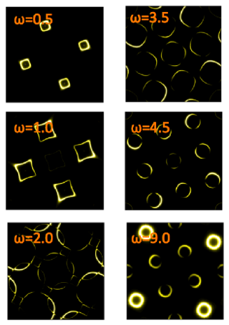
Figure 6: (Color online) Constant-energy cuts (untwinned) of the dynamic structure factor $S^{in}(k,\omega)$ for parameters: $J_{1}=-1$, $J_{1}^{\prime}=0.2$, $J_{2}=1$ and $J_{2}^{\prime}=2.5$, (ii)$J_{1}=-1.5$. The x-axis and y-axis correspond to $3k_{x}-k_{y}$ and $k_{x}+3k_{y}$ direction in range ($-\pi$,$\pi$) respectively. The constant-energy cuts from top to down = 0.5$J_{2}$ , 1.0$J_{2}$, 2.0$J_{2}$, 3.5$J_{2}$, 5.0$J_{2}$ and 9.0$J_{2}$ for the all the energy range.

Fig. 6 shows our predictions for the intensity of the dynamical structure factor of the block checkerboard antiferromagnetic order(an untwinned case) as a function of frequency. At low energies($\omega=0.5$), four strongest quadrate diffraction peaks are visible, which come from the acoustic spin-wave branch. With the increasing of the cut frequency($\omega=1$), four strongest quadrate diffraction peaks disperse outward toward, which is also in the acoustic spin-wave branch range. At intermediate frequency($\omega=2$), the dynamic structure factor becomes a chain ring shape diffraction peaks, which is a common results of acoustic and the third optical spin-wave branch. However, the intensity of diffraction peaks around the $\Gamma$ point is very weak. At high frequency($\omega=3.5$), the chain ring shape evolves to nine strong circle diffraction peaks, which come from the two optical spin-wave branch, which is degenerate in the $\Gamma$ point. But the intensity of diffraction peaks around the $\Gamma$ point is also very weak. Different from the low energy situation, in the higher frequency($\omega=4.5$), the nine strong circle diffraction peaks don’t disperse outward toward, but inward toward; simultaneously, the middle circle diffraction peak around the $\Gamma$ point becomes weaker and vanishes with the increasing of the cut energy. The diffraction peak at this energy cut come from the two optical spin-wave branches, which is degenerate in $\Gamma$ the point. At highest frequency($\omega=9.0$), four strongest circle diffraction peaks are visible at the four corners of extended BZ for one block and four weaker circle diffraction peaks are visible around the $\Gamma$ point and the middle of the four boundaries, which come from the first optical spin-wave branch. The results are similar for other sets of parameters that have same ground states, with the main difference being that the energy cuts must be changed to obtain the similar spin dynamical factor patten.

IV Discussions and Conclusions

In conclusion, starting with the $J_{1}-J_{2}$ Heisenberg Hamiltonian model, we have obtained the magnetic ground state phase diagram by MQ approach and found that the block checkerboard antiferromagnetic order is stable at reasonable physical parameter region. In this paper, we have used spin wave theory to investigate the spin wave and dynamic structure factor for the block checkerboard antiferromagnetic state observed in the iron-based superconductors. There are two acoustic branches and six optical branches spin wave in the block checkerboard antiferromagnetic spin system, which are the combination by the ’molecular orbital’ in the $\Gamma$ point. Then, we discussed the saddlepoint structure in the magnetic excitation spectrum, which can also be measured by neutron scattering experiments. The explicit analytical expressions for the spin-wave dispersion spectra at $\Gamma$ and $k=(\frac{\pi}{\sqrt{10}a},\frac{\pi}{\sqrt{10}a})$ have been given. Comparison with future inelastic neutron scattering studies, we can obtain the specific values of interaction parameters. We have also calculated the predicted inelastic neutron scattering pattern based on linear spin wave theory. In addition, we have also studied the specific influence of each interaction parameter on the spin wave and dynamic structure factor. Neutron scattering experiments about the spin wave and the behavior of spin wave at the proximity of a quantum critical point deserve further attention.

Appendix A Holstein-Primakoff Transformation

The Holstein-Primakoff transformation,

$$\hat{S}_{i}^{\dagger} = (\sqrt{2S-a_{i}^{\dagger}a_{i}})a_{i}\approx\sqrt{2S}a_{i}$$

$$\hat{S}_{i}^{-} = a_{i}^{\dagger}(\sqrt{2S-a_{i}^{\dagger}a_{i}})\approx\sqrt{2S}a_{i}^{\dagger}$$

$$\hat{S}_{i}^{z} = \left(S-a_{i}^{\dagger}a_{i}\right)$$ (5)

for $i=1,2,3,4$, which is occupied by spin up; S represents the size of the magnetic moment for each iron.

and

$$\hat{S}_{-i}^{\dagger} = b_{-1}^{\dagger}(\sqrt{2S-b_{-i}^{\dagger}b_{-i}})\approx\sqrt{2S}b_{-i}^{\dagger}$$

$$\hat{S}_{-i}^{-} = (\sqrt{2S-b_{-i}^{\dagger}b_{-i}})b_{-i}\approx\sqrt{2S}b_{-i}$$

$$\hat{S}_{-i}^{z} = \left(b_{-i}^{\dagger}b_{-i}-S\right)$$ (6)

for $i=1,2,3,4$, which is occupied by spin down.

The fourier transform for bosonic operators is,

$$a_{L} = N^{\frac{1}{2}}\Sigma_{k}e^{ik\cdot R_{L}}a_{k}$$

$$a_{L}^{\dagger} = N^{\frac{1}{2}}\Sigma_{k}e^{-ik\cdot R_{L}}a_{k}^{\dagger}$$

$$b_{L} = N^{\frac{1}{2}}\Sigma_{k}e^{ik\cdot R_{L}}b_{k}$$

$$b_{L}^{\dagger} = N^{\frac{1}{2}}\Sigma_{k}e^{-ik\cdot R_{L}}b_{k}^{\dagger}$$ (7)

Here, we define N is the number of the magnetic unit cell. $L$ is the site index and k is momentum index.

Appendix B Spin Wave Hamiltonian

We write the detailed expression in Eq. 2. Replacing the spin operators by HP bosons, we can get the HP boson Hamiltonian $\mathcal{H}_{k}$,

$$\begin{smallmatrix}\left\{\begin{array}[]{cccccccc}E_{1}&F_{k}&G_{k}&S_{k}&0&\left(B_{k}\right)^{*}&\left(C_{k}\right)^{*}&\left(A_{k}\right)^{*}\\ \left(F_{k}\right)^{*}&E_{1}&S_{k}&T_{k}&B_{k}&0&\left(A_{k}\right)^{*}&\left(D_{k}\right)^{*}\\ \left(G_{k}\right)^{*}&\left(S_{k}\right)^{*}&E_{1}&(F_{k})^{*}&C_{k}&A_{k}&0&B_{k}\\ \left(S_{k}\right)^{*}&\left(T_{k}\right)^{*}&F_{k}&E_{1}&A_{k}&D_{k}&\left(B_{k}\right)^{*}&0\\ 0&(B_{k})^{*}&(C_{k})^{*}&(A_{k})^{*}&E_{1}&F_{k}&G_{k}&S_{k}\\ B_{k}&0&(A_{k})^{*}&(D_{k})^{*}&(F_{k})^{*}&E_{1}&S_{k}&T_{k}\\ C_{k}&A_{k}&0&B_{k}&(G_{k})^{*}&(S_{k})^{*}&E_{1}&\left(F_{k}\right)^{*}\\ A_{k}&D_{k}&(B_{k})^{*}&0&(S_{k})^{*}&(T_{k})^{*}&F_{k}&E_{1}\end{array}\right\}\end{smallmatrix}$$

and

$$\begin{smallmatrix}E_{k}&=&J_{1}+1J^{\prime}_{1}-1J_{2}+2J^{\prime}_{2}\\ A_{k}&=&J^{\prime}_{2}Se^{-i\overrightarrow{k}\cdot\overrightarrow{x_{a}}}\\ B_{k}&=&J^{\prime}_{2}Se^{i\overrightarrow{k}\cdot\overrightarrow{y_{a}}}\\ C_{k}&=&J^{\prime}_{1}Se^{-i\overrightarrow{k}\cdot(0.5\overrightarrow{x_{a}}+0.5\overrightarrow{y_{a}})}\\ D_{k}&=&J^{\prime}_{1}Se^{i\overrightarrow{k}\cdot(0.5\overrightarrow{x_{a}}-0.5\overrightarrow{y_{a}})}\\ F_{k}&=&SJ_{1}e^{-i\overrightarrow{k}\cdot(0.5\overrightarrow{x_{a}}-0.5\overrightarrow{y_{a}})}\\ G_{k}&=&SJ_{2}e^{-i\overrightarrow{k}\cdot\overrightarrow{x_{a}}}\\ S_{k}&=&SJ_{1}e^{-i\overrightarrow{k}\cdot(0.5\overrightarrow{x_{a}}+0.5\overrightarrow{y_{a}})}\\ T_{k}&=&SJ_{2}e^{-i\overrightarrow{k}\cdot\overrightarrow{y_{a}}}\\ \overrightarrow{x_{a}}&=&\sqrt{1.6}a\overrightarrow{i}+\sqrt{0.4}a\overrightarrow{j}\\ \overrightarrow{y_{a}}&=&-\sqrt{0.4}a\overrightarrow{i}+\sqrt{1.6}a\overrightarrow{j}\end{smallmatrix}$$

In the ’molecular orbital’ basis, the Hamiltonian $\mathcal{H}^{orbital}_{k}$ becomes,

$$\begin{smallmatrix}\frac{1}{4}\left\{\begin{array}[]{cccccccc}E_{o}^{1}&0&0&0&A_{o}&B_{o}&C_{o}&D_{o}\\ 0&E_{o}^{2}&0&0&\left(B_{o}\right)^{*}&F_{o}&-D_{o}&G_{o}\\ 0&0&E_{o}^{3}&0&\left(C_{o}\right)^{*}&-D_{o}&P_{o}&S_{o}\\ 0&0&0&E_{o}^{4}&D_{o}&\left(G_{o}\right)^{*}&\left(S_{o}\right)^{*}&T_{o}\\ A_{o}^{4}&B_{o}&C_{o}&D_{o}&E_{o}^{1}&0&0&0\\ \left(B_{o}\right)^{*}&F_{o}&-D_{o}&G_{o}&0&E_{o}^{2}&0&0\\ \left(C_{o}\right)^{*}&-D_{o}&P_{o}&S_{o}&0&0&E_{o}^{3}&0\\ D_{o}&\left(G_{o}\right)^{*}&\left(S_{o}\right)^{*}&T_{o}&0&0&0&E_{o}^{4}\end{array}\right\}\end{smallmatrix}$$

and

$$\begin{smallmatrix}E_{o}^{1}&=&-16J_{1}+4J^{\prime}_{1}+8.J^{\prime}_{2}\\ E_{o}^{2}&=&-8J_{1}+4J^{\prime}_{1}-8J_{2}+8J^{\prime}_{2}\\ E_{o}^{3}&=&-8J_{1}+4J^{\prime}_{1}-8J_{2}+8J^{\prime}_{2}\\ E_{o}^{4}&=&4J^{\prime}_{1}+8J^{\prime}_{2}\\ A_{o}&=&[2J^{\prime}_{1}-4J^{\prime}_{2}].[cos(a_{o})+cos(b_{o})]\\ B_{o}&=&-2J^{\prime}_{1}[sin(a_{o})+sin(b_{o})]i\\ &&+4J^{\prime}_{2}sin(b_{o})i\\ C_{o}&=&-2J^{\prime}_{1}[sin(a_{o})-sin(b_{o})]i\\ &&+4J^{\prime}_{2}sin(a_{o})i\\ D_{o}&=&2J^{\prime}_{1}[cos(a_{o})-cos(b_{o})]\\ F_{o}&=&-2J^{\prime}_{1}[cos(a_{o})+cos(b_{o})]\\ &&-4J^{\prime}_{2}[cos(a_{o})-cos(b_{o})]\\ G_{o}&=&2J^{\prime}_{1}[sin(a_{o})-sin(b_{o})]i\\ &&+4J^{\prime}_{2}sin(a_{o})i\\ P_{o}&=&4J^{\prime}_{2}[cos(a_{o})-cos(b_{o})]]\\ &&-2J^{\prime}_{1}[cos(a_{o})+cos(b_{o})\\ S_{o}&=&4J^{\prime}_{2}sin(b_{o})i\\ &&+2J^{\prime}_{1}[sin(a_{o})+sin(b_{o})]i\\ T_{o}&=&[2J^{\prime}_{1}+4J^{\prime}_{2}].[cos(a_{o})+cos(b_{o})]\\ a_{o}&=&1.5\overrightarrow{k}\cdot\overrightarrow{x_{a}}+0.5\overrightarrow{k}\cdot\overrightarrow{y_{a}}\\ b_{o}&=&0.5\overrightarrow{k}\cdot\overrightarrow{x_{a}}-1.5\overrightarrow{k}\cdot\overrightarrow{y_{a}}\end{smallmatrix}$$

The matrix elements for different ’molecular orbital’ in the same block is zero.

Appendix C Numerical Diagonalization Method

We can use the numerical method to diagonalize the boson pairing Hamiltonian. The matrix form for boson Hamiltonian is,

$$\psi^{\dagger}\hat{\mathbb{\mathcal{H}}}\psi = \left[a^{\dagger},b\right]\left[\begin{array}[]{cc}A&B\\ B&A\end{array}\right]\left[\begin{array}[]{c}a\\ b^{\dagger}\end{array}\right]$$

Here, $\psi^{\dagger}=\left(a^{\dagger},b\right)=\left(a_{1}^{\dagger},a_{2}^{\dagger},a_{3}^{\dagger},a_{4}^{\dagger},b_{-1},b_{-2},b_{-3},b_{-4}\right)$, A and B is a $4\times 4$ matrix; a and b are boson operators. The operators satisfy the commutation relation,

$$\left[\psi_{i},\psi_{j}^{\dagger}\right] = \hat{I}_{-i,j}$$

and

$$\hat{I}_{-} = \left(\begin{array}[]{cc}I&0\\ 0&-I\end{array}\right)$$

$I$ is a $4\times 4$ identity matrix.

The diagonalization problem amounts to finding a transformation $T$, which lets $\hat{T}^{\dagger}\hat{\mathcal{H}}\hat{T}$ become a diagonalization matrix $\Omega$.

$$\psi = \left[\begin{array}[]{c}a\\ b^{\dagger}\end{array}\right]=\hat{T}\left[\begin{array}[]{c}\alpha\\ \beta^{\dagger}\end{array}\right]=\hat{T}\varphi$$

Here, we require that $\alpha$ and $\beta$ are also a set of boson operators and $\varphi^{\dagger}=\left(\alpha^{\dagger},\beta\right)=\left(\alpha_{1}^{\dagger},\alpha_{2}^{\dagger},\alpha_{3}^{\dagger},\alpha_{4}^{\dagger},\beta_{-1},\beta_{-2},\beta_{-3},\beta_{-4}\right)$.

Then,

$$\left[\psi_{i},\psi_{j}^{\dagger}\right] = \hat{I}_{-i,j}=\sum_{i^{\prime},j^{\prime}}T_{i,i^{\prime}}I_{-i^{\prime},j^{\prime}}T_{j^{\prime},j}^{\dagger}$$

we get

$$\hat{T}\hat{I}_{-}\hat{T}^{\dagger}=\hat{I}_{-}$$ (11)

Since $\hat{I}_{-}^{2}=I$. we know $I=(\hat{I}_{-}\hat{T})(\hat{I}_{-}\hat{T}^{\dagger})$. Due to $(\hat{I}_{-}\hat{T})$ and $(\hat{I}_{-}\hat{T}^{\dagger})$ are each inverses, thus $I=(\hat{I}_{-}\hat{T}^{\dagger})(\hat{I}_{-}\hat{T})$ and $\hat{T}^{\dagger}\hat{I}_{-}\hat{T}=\hat{I}_{-}$.

Then we want the final form of $\hat{\mathcal{H}}$ is diagonalization.

$$\hat{\mathcal{H}} = \left[a^{\dagger},b\right]\left[\begin{array}[]{cc}A&B\\ B&A\end{array}\right]\left[\begin{array}[]{c}a\\ b^{\dagger}\end{array}\right]$$

$$= \psi^{\dagger}\hat{\mathbb{\mathcal{H}}}\psi$$

$$= \varphi^{\dagger}\left\{\hat{T}^{\dagger}\left[\begin{array}[]{cc}A&B\\ B&A\end{array}\right]\hat{T}\right\}\varphi$$ (19)

$$= \left[\alpha^{\dagger},\beta\right]\left\{\hat{T}^{\dagger}\left[\begin{array}[]{cc}A&B\\ B&A\end{array}\right]\hat{T}\right\}\left[\begin{array}[]{c}\alpha\\ \beta^{\dagger}\end{array}\right]$$ (24)

$$= \left[\alpha^{\dagger},\beta\right]\left\{\hat{\Omega}\right\}\left[\begin{array}[]{c}\alpha\\ \beta^{\dagger}\end{array}\right]$$

$$= \varphi^{\dagger}\hat{\Omega}\varphi$$

$$= \sum_{i}^{4}\omega_{i}\alpha^{\dagger}\alpha+\omega_{-i}\beta\beta^{\dagger}$$ (28)

Here,$\hat{\Omega}=diag\left(\omega_{1},\cdots,\omega_{4},\omega_{-1},\cdots,\omega_{-4}\right)$ represents a diagonalization matrix and the matrix elements for diagonalization matrix is $\left(\omega_{1},\cdots,\omega_{4},\omega_{-1},\cdots,\omega_{-4}\right)$ .

In other words, we want the expression $\hat{T}^{\dagger}\mathcal{\hat{H}}\hat{T}=\Omega$ and matrix $\hat{\Omega}$ is a diagonalization matrix. We must solve the matrix $\hat{T.}$

Combining Eq.11 and Eq.28, we get,

$$\hat{T}^{\dagger}\mathcal{\hat{H}}\hat{T} = \hat{\Omega}$$

$$\left[\hat{T}\hat{I}_{-}\right]\hat{T}^{\dagger}\mathcal{\hat{H}}\hat{T} = \left[\hat{T}\hat{I}_{-}\right]\hat{\Omega}$$

$$\left[\hat{T}\hat{I}_{-}\hat{T}^{\dagger}\right]\mathcal{\hat{H}}\hat{T} = \left[\hat{T}\hat{I}_{-}\right]\hat{\Omega}$$

$$\hat{I}_{-}\mathcal{\hat{H}}\hat{T} = \left[\hat{T}\hat{I}_{-}\right]\hat{\Omega}$$

$$(\hat{I}_{-}\hat{\mathcal{H}})\hat{T} = \hat{T}\left[\hat{I}_{-}\hat{\Omega}\right]$$

$$(\hat{I}_{-}\hat{\mathcal{H}})\hat{T} = \hat{T}\left[\hat{\lambda}\right]$$ (29)

Here $\hat{\lambda}=\left[\hat{I}_{-}\hat{\Omega}\right]=diag\left(\omega_{1},\cdots,\omega_{4},-\omega_{-1},\cdots,-\omega_{-4}\right)$ is a diagonalization matrix. In other words, if we want to get $\hat{T}^{\dagger}\mathcal{\hat{H}}\hat{T}=\hat{\Omega}$, we can solve the general Hamiltonian $(\hat{I}_{-}\hat{\mathcal{H}})\hat{T}=\hat{T}\left[\hat{\lambda}\right]$.

J.L. van Hemmen’sM-W-Xiao-1 strategy is that the canonical transformation $\hat{T}$ is fully determined by its n(=8) columns {$x_{1}$, … , $x_{1}$, $x_{-1}$, … , $x_{-4}$}. We, therefore, reduce Eq.29 to an eigenvalue problem for these n(=8) vectors $x_{i}$, $1\leqq i\leqq 8$.

Then

$$\left(\hat{I}_{-}\hat{\mathcal{H}}\right)\chi = \lambda\chi$$

Where $\chi=x_{i}$, $1\leqq i\leqq 8$, and $\lambda\in\left\{\omega_{1},\omega_{2},\omega_{3},\omega_{4},-\omega_{-1},-\omega_{-2},-\omega_{-3},-\omega_{-4}\right\}$. So, to diagonalize the Hamiltonian is equivalence to solve a general eigenvalue problem.

If we define a matrix $\hat{I}_{y}=\left[\begin{array}[]{cc}0&I\\ I&0\end{array}\right]$ and $I$ is a $4\times 4$ identity matrix, it is easy to proof ,

$$\hat{I}_{-}\mathcal{\hat{H}} = -\hat{I}_{y}^{-1}\hat{I}_{-}\mathcal{\hat{H}}\hat{I}_{y}$$

We assume there is a eigenvalue $\lambda_{i}$ and eigenvector $\chi_{i}=\left[\begin{array}[]{c}\mu_{1-4}\\ \nu_{1-4}\end{array}\right]$ for the general Hamiltonian,

$$\hat{I}_{-}\hat{\mathcal{H}}\chi_{i} = \lambda_{i}\chi_{i}$$

Then the $\chi^{\prime}_{i}=\hat{I}_{y}\cdot\chi_{i}=\left[\begin{array}[]{c}\nu_{1-4}\\ \mu_{1-4}\end{array}\right]$ is also eigenvector of $\hat{I}_{-}\hat{\mathcal{H}}$ and the corresponding eigenvalue is $\lambda^{\prime}=-\lambda$:

$$\hat{I}_{-}\hat{\mathcal{H}}\chi_{i} = \lambda_{i}\chi_{i}$$

$$-\hat{I}_{y}^{-1}\hat{I}_{-}\hat{\mathcal{H}}\left[\hat{I}_{y}\chi_{i}\right] = \lambda_{i}\chi_{i}$$

$$\hat{I}_{y}\hat{I}_{y}^{-1}\hat{I}_{-}\hat{\mathcal{H}}\left[\hat{I}_{y}\chi_{i}\right] = -\hat{I}_{y}\lambda_{i}\chi_{i}$$

$$\hat{I}_{-}\hat{\mathcal{H}}\left[\hat{I}_{y}\chi_{i}\right] = -\lambda_{i}\hat{I}_{y}\chi_{i}$$

$$I_{-}\hat{\mathcal{H}}\chi^{\prime}_{i} = -\lambda_{i}\chi^{\prime}_{i}$$

$$I_{-}\hat{\mathcal{H}}\chi^{\prime}_{i} = \lambda^{\prime}_{i}\chi^{\prime}_{i}$$

Therefore, the eigenvalue are in pairs. For the sake of convenience, we arrange the order of eigenvalues by the relative size of the value $\aleph_{i}=\mid\mu_{i}\mid^{2}-\mid\nu_{i}\mid^{2}$, ($\aleph_{1}>......>\aleph_{8}$); for the same $\aleph_{i}$, we arrange the order of eigenvalues by its relative size. If the eigenvalue $\lambda_{i}$ for the corresponding eigenvector $\aleph_{1}>\aleph_{2}>\aleph_{3}>\aleph_{4}$ is lower than zero, it represents the ground state is not stable. For the first four eigenvector $\mid\mu_{i}\mid^{2}-\mid\nu_{i}\mid^{2}=1$(i=1,2,3,4) and for the last four eigenvector $\mid\mu_{i}\mid^{2}-\mid\nu_{i}\mid^{2}=-1$ (i=5,6,7,8).

References

- (1) P. A. Lee, N. Nagaosa, and X. G. Wen, Rev. Mod. Phys. 78, 17 (2006).
- (2) J. G. Bednorz, and K. A. Muller, Z. Phys. B 64, 189 (1986).
- (3) Y. Kamihara, T. Watanabe, M. Hirano, and H. Hosono, J. Am. Chem. Soc. 130 3296 (2008).
- (4) G. F. Chen, Phys. Rev. Lett. 101 057007 (2008).
- (5) Hechang Lei, KefengWang, J. B. Warren, andC. Petrovic, arXiv:1102.2215.
- (6) Takeshi Kondo, A. F. Santander-Syro, O. Copie, Chang Liu, M. E. Tillman, E. D. Mun, J. Schmalian, S. L. Bud’ko, M. A. Tanatar, P. C. Canfield, and A. Kaminski, Phys. Rev. Lett., 101, 147003 (2008).
- (7) L. Wray, D. Qian, D. Hsieh, Y. Xia, L. Li, J. G. Checkelsky, A. Pasupathy, K. K. Gomes, C. V. Parker, A. V. Fedorov, G. F. Chen, J. L. Luo, A. Yazdani, N. P. Ong, N. L. Wang, and M. Z. Hasan, Phys. Rev. B, 78, 184508 (2008).
- (8) Gang Xu, Haijun Zhang, Xi Dai, and Zhong Fang, EPL, 84, 67015 (2008).
- (9) S. V. Borisenko, V. B. Zabolotnyy, D. V. Evtushinsky, T. K. Kim, I. V. Morozov, A. N. Yaresko, A. A. Kordyuk, G. Behr, A. Vasiliev, R. Follath, and B. Bhner, Phys. Rev. Lett. 105, 067002 (2010) .
- (10) R. Khasanov, M. Bendele, A. Amato, K. Conder, H. Keller, H.-H. Klauss, H. Luetkens, and E. Pomjakushina, Phys. Rev. Lett. 104, 087004 (2010) .
- (11) J. Guo et al., arXiv:1101.0092 (2011); Y. Kawasaki et al., arXiv:1101.0896 (2011); J. J. Ying et al., arXiv:1101.1234 (2011).
- (12) A. Krzton-Maziopa et al., arXiv:1012.3637 (2010). J. J. Ying et al., arXiv:1012.5552 (2010). A. F. Wang et al., arXiv:1012.5525 (2010) M. Fang et al., arXiv:1012.5236 (2010); H. Wang et al., arXiv:1101.0462 (2011).
- (13) Xun-WangYan, MiaoGao, Zhong-Yi Lu, and TaoXiang, arXiv:1102.2215.
- (14) Wei Bao, G. N. Li, Q. Huang, G. F. Chen, J. B. He, M. A. Green, Y. Qiu, D. M. Wang, J. L. Luo, andM. M. Wu, arXiv:1102.3674.
- (15) Wei Bao, Q. Huang, G. F. Chen, M. A. Green, D. M. Wang, J. B. He X. Q. Wang andY. Qiu, arXiv:1102.0830.
- (16) F. Ye, S. Chi, Wei Bao, X. F. Wang, J. J. Ying, X. H. Chen, H. D. Wang, C. H. Dong, and Minghu Fang,arXiv:1102.2282.
- (17) C. Cao and J. Dai (2011), arXiv:1102.1344.
- (18) V. Yu. Pomjakushin, E. V. Pomjakushina, A. Krzton-Maziopa, K. Conder, and Z. Shermadini, arXiv:1102.3380.
- (19) Yi-ZhuangYou, FangYang, Su-PengKou, and Zheng-YuWeng, arXiv:1102.3200.
- (20) G. M. Zhang, Z. Y. Lu, and T. Xiang, arXiv:1102.4575 (2011).
- (21) A. Auerbach, Phys. Rev. Lett., 72, 2931 (1994).
- (22) E. W. Carlson, D. X. Yao, and D. K. Campbell, Phys. Rev. B , 70, 064505 (2004); D. X. Yao, E. W. Carlson, and D. K. Campbell, Phys. Rev. Lett. 97, 017003 (2006).
- (23) Ming-wen Xiao, arXiv:0908.0787.
- (24) J.L. van Hemmen, Z. Physik B-Condensed Matter 38, 271-277 (1980).
- (25) Lu Huaixin and Zhang Yongde, International Journal of Theoretical Physics, 39, 2, (2000).
- (26) Constantino Tsallis, J. Math. Phys. 19, 277, (1978).
- (27) J.H.P. ColpaCOLPA, Physica A, 93, 327, (1978).