Removable Matter-Power-Spectrum Covariance from Bias Fluctuations

Abstract

We find a simple, accurate model for the covariance matrix of the real-space cosmological matter power spectrum on slightly nonlinear scales ($k\sim$ 0.1-0.8 $h$ Mpc^-1 at $z=0$), where off-diagonal matrix elements become substantial. The model includes a multiplicative, scale-independent modulation of the power spectrum. It has only one parameter, the variance (among realizations) of the variance of the nonlinear density field in cells, with little dependence on the cell size between 2-8 $h^{-1}$ Mpc. Furthermore, we find that this extra covariance can be modeled out by instead measuring the power spectrum of $\delta/\sigma_{\rm cell}$, i.e. the ratio of the overdensity to its dispersion in cells a few Mpc in size. Dividing $\delta$ by $\sigma_{\rm cell}$ essentially removes the non-Gaussian part of the covariance matrix, nearly diagonalizing it.

1. Introduction

The power spectrum of density fluctuations (and its Fourier dual, the correlation function) is the most common statistic used to characterize the large-scale structure of the Universe, and contains much information about cosmological parameters. In linear theory, the power spectrum’s covariance matrix is diagonal, a practical advantage over the correlation function.

However, in the ‘translinear’ regime, the first decade or so in wavenumber smaller than fully linear scales, nonlinearity grows in the density field. The dispersion $\sigma_{\rm cell}$ in the nonlinear overdensity field $\delta$ in cells of translinear size $2\pi/k\sim 4$-60 $h$ Mpc^-1 increases from about 1 to 10 to 20, as $k$ decreases from 60 to 8 to 4 $h$ Mpc^-1, as measured in the simulations analyzed below. (Note that the dispersion in the linearly evolved density field in 8-$h^{-1}$ Mpc cells, $\sigma_{8}\approx 0.8$.)

The growing nonlinearity in $\delta$ incites a substantial non-Gaussian component in its power-spectrum covariance matrix (Meiksin & White, 1999; Scoccimarro et al., 1999; Takahashi et al., 2009, T09). The non-Gaussian covariance leads to a translinear plateau in Fisher information (Rimes & Hamilton, 2005, 2006; Neyrinck et al., 2006; Neyrinck & Szapudi, 2007). When using the power spectrum of $\delta$ to constrain a parameter such as the initial power spectrum amplitude, modes in the translinear regime are highly correlated, giving little additional constraining power when analyzed with larger-scale modes.

A few methods have been proposed that mitigate this problem, to varying degrees: removing large halos from a survey (Neyrinck & Szapudi, 2007); applying a logarithmic or rank-order-Gaussianizing transform to the density field before measuring the power spectrum (Neyrinck et al., 2009; Seo et al., 2011; Yu et al., 2011); and nonlinear wavelet Wiener filtering (Zhang et al., 2011).

The non-diagonality of the power-spectrum covariance matrix is not just a problem for parameter estimation. Without a theoretical model, off-diagonal elements must be estimated numerically, often cumbersomely. Even a covariance matrix estimated with 5000 simulations leaves residual noise (T09; see Fig. 4 below). Also, the results often depend on the method used to measure the covariance. For example, spatial jackknife resampling systematically underpredicts the covariance (Norberg et al., 2009). Another strategy, which we employ, applies a large set of sinusoidal weighting functions to a single density field (Hamilton et al., 2006, HRS). The HRS weightings are designed to be optimally friendly to Fourier modes smaller than the sinusoids themselves, unlike windows with sharp configuration-space edges. Any window function introduces ‘beat coupling’ between small and large-scale modes; this contributes off-diagonal covariance beyond what is found in an ensemble of unweighted, periodic simulations. For the sinusoidal weightings, the beat coupling likely does not exceed that for more-disruptive, sharp window functions, often present in observations. Another recent technique to generate low-noise covariance matrices from a relatively small number of simulations makes use of ‘mode-resampling’ (Schneider et al., 2011), taking advantage of the plethora of small-scale modes available.

‘Shrinkage estimation’ (Pope & Szapudi, 2008) is possible if an approximate model is known for the covariance; this gives an optimal combination of a noiseless but idealized model, and a complete but noisy measured covariance matrix. One popular theoretical model for the covariance uses a halo-model (HM) framework (Cooray & Hu, 2001). The full HM covariance includes up to four-halo terms, and requires knowledge of the halo-halo power spectrum, bi- and trispectrum. Unfortunately, even the halo-halo power spectrum currently lacks a satisfying analytical model (Smith et al., 2007). Leading-order perturbation-theory power, bi-, and trispectra can be used, but on translinear scales they are likely inaccurate for halo-halo correlations, making their nontrivial implementation possibly not worth the trouble. Thus, in practice often only the simpler 1-halo term is used.

In this paper, we explore a simple, accurate model for translinear covariance from a fluctuating multiplicative bias. Sato et al. (2009) considered a term with a rather similar form to this, called ‘halo sampling variance’ (HSV), consisting of a variance in bias multiplying one-halo power-spectrum terms. They found that including this HSV, which, unlike us, they ascribe to modes outside the survey volume, was necessary to model the covariance of the weak-lensing convergence power spectrum accurately in a halo-model approach.

2. Results

We measured real-space power spectra and covariance matrices from the Coyote Universe (Heitmann et al., 2010, 2009; Lawrence et al., 2010) suite of 37 simulations. Each of these has a different set of cosmological parameters, each of them a plausible (given current observational constraints) concordance $\Lambda$CDM model. The simulations occupy an orthogonal-array-Latin-hypercube in the five-dimensional parameter space $\Omega_{m}h^{2}\in[0.12,0.155]$, $\Omega_{b}h^{2}\in[0.0215,0.0235]$, $n_{s}\in[0.85,1.05]$, $w\in[-1.3,-0.7]$, $\sigma_{8}\in[0.61,0.9]$. The remaining cosmological parameters, e.g. $h$, are set to match the tight cosmic microwave background (CMB) constraint on the ratio of the last-scattering-surface distance to the sound-horizon scale. The 1024³-particle simulations have box size 1300 Mpc, fixed in Mpc (not  $h^{-1}$ Mpc) to roughly line up baryon-acoustic-oscillation (BAO) features in $k$ among different cosmologies. Their resolution is sufficient for power-spectrum measurements accurate at sub-percent level at scales down to $k=1$ $h$ Mpc^-1. We measured power spectra on grids with nearest-grid-point density assignment, not correcting for the pixel window function on the $128^{3}$-$512^{3}$ grids we use.

The variable set of cosmologies prevented estimating covariances by directly comparing power spectra among simulations. So, we measured covariances within each simulation separately, using 248 (combinations of no weighting, and the first and second overtones in each Cartesian direction) sinusoidal weightings prescribed by HRS. We then averaged the covariance matrices from different cosmologies together to reduce noise. Arguably, mixing cosmologies in this way is a good thing, decreasing the dependence on cosmological parameters.

We did not use the covariance of the power spectrum $P$ itself, but of $\ln P$, defining $C_{ij}\equiv\left\langle{\Delta\ln P_{i}\Delta\ln P_{j}}\right\rangle=\left\langle{\Delta P_{i}\Delta P_{j}}\right\rangle/\left\langle{P_{i}}\right\rangle\left\langle{P_{j}}\right\rangle$. Averaging this covariance matrix across cosmologies is more stable than the covariance matrix of $P$ itself. We also define the quantity $T_{ij}\equiv C_{ij}(N_{i}N_{j})^{1/2}-2\delta^{K}_{ij}$, where $\delta^{K}_{ij}$ is a unit matrix, and $N_{i}$ is the number of modes in bin $i$. $T_{ij}$, zero for a Gaussian random field, is a measure of the non-Gaussian component of a covariance matrix, normalized to the Gaussian component. Conveniently for plotting purposes, it has roughly uniform noise properties.

Figure 1.— Pixels are colored according to the quantities listed on the left edge of the plots; for quantities exceeding 1, contours appear at successive powers of 2. Top row. The normalized non-Gaussian part of the covariance matrix $T_{ij}$. Middle row. An approximation to $T_{ij}$, using $\alpha={\rm Var}(\sigma^{2}_{\rm cell})/\sigma^{4}_{\rm cell}$, measured from each simulation’s ensemble of sinusoidal weightings, and geometrically averaged across simulations. Bottom row. $T_{ij}$ for the power spectrum normalized by the cell-density variance, $P(k)/\sigma^{2}_{\rm cell}$, equivalent to the power spectrum of $(\delta/\sigma_{\rm cell})$. (The displayed range of $k$ includes modes not directly modulated by the weightings, and below the Nyquist $k$. The cell sizes are 1300/128, 1300/256 and 1300/512 Mpc, roughly the listed values in $h^{-1}$ Mpc.)

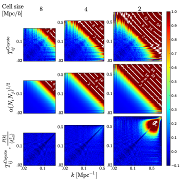
The top row of Fig. 1 shows $T_{ij}$, measured from the simulations. As the middle row shows, $T_{ij}$ is well-approximated by $T_{ij}=\alpha(N_{i}N_{j})^{1/2}$, for $\alpha={\rm Var}(\sigma^{2}_{\rm cell})/\sigma^{4}_{\rm cell}$. Here ${\rm Var}(\sigma^{2}_{\rm cell})$ is the variance of the measured (not linear-theory) cell-density variance $\sigma^{2}_{\rm cell}$ among sinusoidally weighted density fields. $\alpha$, proportional to a variance, is inversely proportional to the volume $V=(1.3\ {\rm Gpc})^{3}/2$ (the sinusoidal weightings effectively halve the volume).

The approximate form of this covariance matrix is that of a Gaussian field, with additional power proportional to a scale-independent bias. Consider a field with power spectrum $P_{i}=b\left\langle{P_{i}}\right\rangle+P^{G}_{i}$. Here $P^{G}$ is the power spectrum of a Gaussian random field such that $\left\langle{P_{i}}\right\rangle=\left\langle{P^{G}_{i}}\right\rangle$, and $b$ is a variable scale-independent bias, uncorrelated with fluctuations in $P^{G}$, with $\left\langle{b}\right\rangle=0$. (Suppose $b>-1$, e.g. is lognormally distributed, to avoid $P_{i}<0$.) $P$’s covariance matrix is

$$C_{ij}=\left\langle{b^{2}}\right\rangle\left\langle{P_{i}}\right\rangle\left\langle{P_{j}}\right\rangle+\left\langle{\Delta P^{G}_{i}\Delta P^{G}_{j}}\right\rangle.$$ (1)

$\left\langle{\Delta P^{G}_{i}\Delta P^{G}_{j}}\right\rangle=2\delta^{K}_{ij}P_{i}^{2}/N_{i}$, so $T_{ij}=\left\langle{b^{2}}\right\rangle(N_{i}N_{j})^{1/2}$. Neglecting fluctuations from $P^{G}$, $\sigma^{2}_{\rm cell}=\left\langle{b^{2}}\right\rangle\sigma^{4}_{\rm cell}$. Here the proportionality constant $\alpha=\left\langle{b^{2}}\right\rangle$.

With the insight that the covariance is from bias fluctuations, perhaps the covariance can be removed. Indeed, in the bottom row of Fig. 1, we show that the translinear covariance largely vanishes if the power spectrum from each density field is divided by $\sigma^{2}_{\rm cell}$, measured from that field. This is equivalent to measuring the power spectrum of ($\delta/\sigma_{\rm cell}$). The reduction in covariance is dramatic for cell sizes $\gtrsim 4$ $h^{-1}$ Mpc. Using 2-$h^{-1}$ Mpc cells, there is significant residual covariance on small scales, but the covariance is still much smaller than in the top rows. Interestingly, $\alpha$ is quite consistent over this factor of 4 in cell size; with 2, 4, and 8 $h^{-1}$ Mpc cells, $\alpha\times 10^{4}$=1.29, 1.37 and 1.22.

Figure 2.— Correlation matrices of various power spectra measured from the Coyote Universe simulations. $P_{\delta}$ is the conventional power spectrum; $P_{\delta}/\sigma^{2}_{\rm cell}$ is the power spectrum, dividing by the variance of cell densities; $P_{\ln(1+\delta)}$ is the power spectrum of the log-density; $P_{G(\delta)}$ is the power spectrum of the Gaussianized density.

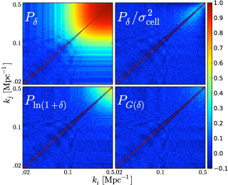
Fig. 2 shows a commonly plotted measure of the covariance, the correlation matrix $C_{ij}/(C_{ii}C_{jj})^{1/2}$. $P_{\delta}/\sigma^{2}_{\rm cell}$ has smaller covariance even than the $\ln(1+\delta)$ power spectrum (NSS09), surpassed in diagonality only by the Gaussianized power spectrum (NSS09). Hereafter, all of the Coyote Universe results use a 256³ grid, with a cell size of $\sim 4$ $h^{-1}$ Mpc.

We note that the form of the $\ln(1+\delta)$ covariance matrix is similar to the $\delta$ covariance matrix, except that the constant $\alpha$ is given by fluctuations in the variance of $\ln(1+\delta)$ in cells. This sheds light on the reduction in covariance from transforming the density to give a more-Gaussian 1-point distribution. By definition, Gaussianization reduces higher moments, in particular the kurtosis, and thus the variance in the variance. In our model, then, the full power-spectrum covariance is reduced.

2.1. Comparison with the halo model

Figure 3.— The non-Gaussian part of the covariance, $C^{\rm NG}_{ij}$, in the halo model, including just the 1-halo term (left panel), and with all terms (middle panel). $C^{\rm NG}_{ij}$ as measured in the Coyote Universe simulations appears in the right panel. In all cases, $C^{\rm NG}_{ij}$ is divided by $\alpha={\rm Var}(\sigma^{2}_{\rm cell})/\sigma^{4}_{\rm cell}$, measured from the simulations.

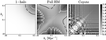
Fig. 3 shows the quantity $C^{\rm NG}_{ij}\equiv C_{ij}-2\delta^{K}_{ij}/(N_{i}N_{j})^{1/2}$, the covariance minus the Gaussian component; this should be a constant in our $\alpha$ model. We compare $C^{\rm NG}_{ij}$ as measured from the Coyote Universe to predictions in the HM, both using all terms, and only the 1-halo term. For the HM covariance matrix we use our CosmoPy implementation (Neyrinck et al., 2006; Neyrinck & Szapudi, 2007, 2008). In all panels, $C^{\rm NG}_{ij}$ is normalized by dividing by $\alpha$ as measured in the simulations.

Indeed, at large $k$, the measured $C^{\rm NG}_{ij}/\alpha\approx 1$, conforming to the form above. For the HM panels, we set $N_{i}\propto k^{2}$ exactly; i.e. fluctuations in $N_{i}$ from the finite lattice are suppressed for clarity. The detailed features in the HM $C^{\rm NG}_{ij}$ are different than that measured. On large scales, where there is much noise in the measured $C^{\rm NG}_{ij}$, there is barely a hint of the perturbation-theory trispectrum wiggles from BAO (Neyrinck & Szapudi, 2008). This is not surprising; in that paper it took a few hundred Gpc-scale simulations to get a clear signal.

While our simple model involving $\alpha$ seems more accurate than the HM covariances on translinear scales, the HM does not fail utterly; the full-HM covariance is typically within a factor of two of that measured. Given that we did not adjust HM parameters or polyspectrum assumptions to optimize the fit, its agreement is not bad. The agreement with the commonly used 1-halo covariance, however, is poorer outside the large-$k$ corner. This vanilla 1-halo model assumes a halo mass function with uncorrelated Poisson fluctuations in each mass bin (Neyrinck et al., 2006); perhaps including mass-function covariance would improve agreement.

2.2. Comparison with other results

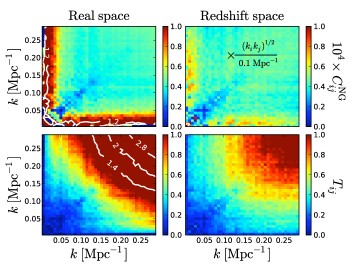
It is well worth checking our result with other covariance measurements, given our averaging procedure over cosmologies, and the ‘beat-coupling’ induced by our sinusoidal weightings. Fig. 4 shows measurements by T09 of $T_{ij}$ and $C^{\rm NG}_{ij}$ from their suite of 5000 $\Lambda$CDM simulations of volume 1 ($h^{-1}$ Gpc)³, each with 256³ particles.

Figure 4.— Real- and redshift-space non-Gaussian covariances $C^{\rm NG}_{ij}$ and $T_{ij}$ measured from an ensemble of 5000 simulations by T09. The redshift-space $C^{\rm NG}_{ij}$ is additionally multiplied by an empirically found factor $\propto(k_{i}k_{j})^{1/2}$ to become roughly constant for large $k$. Note the linear $k$ scale.

For $k\gtrsim 0.04$ $h$ Mpc^-1, the real-space $C^{\rm NG}_{ij}$ is roughly constant, in accordance with our model. However, for smaller $k$, $C^{\rm NG}_{ij}$ roughly doubles from its smaller-scale value; unsurprisingly, other effects take over on the largest scales. As in the Coyote Universe results, at BAO scales there are interesting depressions in the covariance near the diagonal, where the covariance even dips slightly negative. In Fig. 4 there is also a suggestion of periodic BAO bumps along the axes.

In redshift space, we found empirically that $C^{\rm NG}_{ij}$ instead falls off roughly as $(k_{i}k_{j})^{-1/2}$. We do not speculate here on why it has this form, but the reduced redshift-space covariance on small scales, noted by T09, is not surprising given the more-Gaussian redshift-space density 1-point distribution, smeared by redshift distortions (Neyrinck et al., 2011).

2.3. Fisher information

Fig. 5 shows signal-to-noise, (S/N)², curves for the various power spectra. This (S/N)² can be thought of as the effective number of independent modes over a range of wavenumber bins $\mathcal{R}$.

$$({\rm S/N})^{2}(\mathcal{R})=\sum_{i,j\in\mathcal{R}}(\textbf{{C}}_{\mathcal{R}}^{-1})_{ij},$$ (2)

where $\textbf{{C}}_{\mathcal{R}}$ is the covariance matrix over $\mathcal{R}$. Here, the bins in $\mathcal{R}$ vary from $k_{\rm min}$, the largest modes not directly modulated by the sinusoidal weightings, to $k_{\rm max}$.

Figure 5.— The intrinsic Fisher information, (S/N)², in various power spectra, measured from the Coyote Universe simulations. The dotted curve uses our model for the $P_{\delta}$ covariance from fluctuations in a scale-independent multiplicative bias.

Compared to NSS09, the range of $k$ plotted here is shifted smaller by a factor of 2 by the double box size, and there is reduced noise, but the trends are the same as found there. In fact, $P_{\delta}/\sigma^{2}_{\rm cell}$ is comparable to $P_{G(\delta)}$, the power spectrum of the Gaussianized density. The (S/N)² in $P_{\delta}/\sigma^{2}_{\rm cell}$ ramps up quickly at the smallest scales, because the power spectra are effectively pinned together there when they are divided by $\sigma^{2}_{\rm cell}$, resulting in tiny (co)variance. We also show the (S/N)² curve for our $C^{\rm NG}_{ij}=\alpha$ model, which approximates the $P_{\delta}$ curve well.

(S/N)² is a good single measure of intrinsic Fisher information, but without derivative terms of the power spectrum with respect to cosmological parameters, the connection with parameter estimation is vague. For $P_{\delta}$, (S/N)² is roughly the information in $\ln\sigma_{8}^{2}$, unmarginalized over other parameters, since on linear scales $\partial P_{\delta}(k)/(\partial\ln\sigma_{8}^{2})=1$, and it stays of order unity on non-linear scales, reaching $\sim 2$ (Neyrinck & Szapudi, 2007). However, at least for 8-$h^{-1}$ Mpc cells, $P_{\delta}/\sigma^{2}_{\rm cell}$ contains little information about $\sigma_{8}^{2}$. (If the measured power spectrum were linear, obviously all sensitivity to $\sigma_{8}^{2}$ would be lost in dividing by it.) For $P_{G(\delta)}$, too, a free parameter is the variance in the Gaussianized density. In the present measurements, as in Neyrinck et al. (2011), the $G(\delta)$ variance is fixed, pinning down the power spectrum at small scales in a similar manner as with $P_{\delta}/\sigma^{2}_{\rm cell}$. The situation with $P_{\ln(1+\delta)}$ is in-between; on small scales it is allowed to fluctuate as it pleases (which is to a much lesser degree than $P_{\delta}$), but on large scales, $0<\partial P_{\ln(1+\delta)}/(\partial\ln\sigma_{8}^{2})<1$ because of large-scale bias produced by the log transform.

An analysis of these issues (Neyrinck, 2011, in prep.) is essential for these modified power spectra to be used for cosmological constraints. One might think that the insight that $P_{\delta}$’s covariance is largely from fluctuations in a multiplicative bias might imply that this covariance is unimportant for parameters that depend on the power-spectrum shape, such as the tilt, or the BAO scale. However, as shown in Fig. 4, the form we have found for the translinear covariance does not really extend to fully linear scales, leaving some room for shape fluctuations at the interface (occupied by BAO at $z=0$) between the linear and translinear regimes.

3. Conclusion

We show that a fluctuating scale-independent multiplicative bias provides quite an accurate model for the covariance matrix of the real-space dark-matter power spectrum on translinear scales. The non-Gaussian part of the covariance $C^{\rm NG}_{ij}\approx\alpha={\rm Var}(\sigma^{2}_{\rm cell})/\sigma^{4}_{\rm cell}$, a constant measure of the variance (among realizations) of the variance (within a realization) of the measured nonlinear density field. $\alpha$ is rather insensitive to the cell size used to measure it, at least within a range of 2-8 $h^{-1}$ Mpc. $\alpha$ is not entirely trivial to measure, but it is much easier than the full covariance. For example, it could be estimated using sufficiently large simple sub-volumes, with little worry about edge effects.

Furthermore, at least in real space, this translinear covariance can largely be removed, or modeled out, by dividing the power spectrum by $\sigma^{2}_{\rm cell}$. This is equivalent to measuring the power spectrum of $\delta/\sigma_{\rm cell}$. However, this changes the sensitivity to cosmology, for example giving up information on the power-spectrum amplitude.

The simplicity of this model suggests that it may be applicable not only to dark matter, but perhaps to galaxies, or even to CMB anisotropies, where pushing to smaller scales dredges up some non-Gaussian covariance in the power spectrum of Sunyaev-Zel’dovich effect anisotropies (Shaw et al., 2009). Shot noise would complicate the situation for galaxies, but possibly this component could be accurately approximated with a Poisson term and subtracted.

References

- Cooray & Hu (2001) Cooray, A., & Hu, W. 2001, ApJ, 554, 56, arXiv:astro-ph/0012087
- Hamilton et al. (2006) Hamilton, A. J. S., Rimes, C. D., & Scoccimarro, R. 2006, MNRAS, 371, 1188, arXiv:astro-ph/0511416
- Heitmann et al. (2009) Heitmann, K., Higdon, D., White, M., Habib, S., Williams, B. J., Lawrence, E., & Wagner, C. 2009, ApJ, 705, 156, 0902.0429
- Heitmann et al. (2010) Heitmann, K., White, M., Wagner, C., Habib, S., & Higdon, D. 2010, ApJ, 715, 104, 0812.1052
- Lawrence et al. (2010) Lawrence, E., Heitmann, K., White, M., Higdon, D., Wagner, C., Habib, S., & Williams, B. 2010, ApJ, 713, 1322, 0912.4490
- Meiksin & White (1999) Meiksin, A., & White, M. 1999, MNRAS, 308, 1179, arXiv:astro-ph/9812129
- Neyrinck (2011, in prep.) Neyrinck, M. C. 2011, in prep.
- Neyrinck & Szapudi (2007) Neyrinck, M. C., & Szapudi, I. 2007, MNRAS, 375, L51, arXiv:astro-ph/0610211
- Neyrinck & Szapudi (2008) ——. 2008, MNRAS, 384, 1221, arXiv:0710.3586
- Neyrinck et al. (2006) Neyrinck, M. C., Szapudi, I., & Rimes, C. D. 2006, MNRAS, 370, L66, arXiv:astro-ph/0604282
- Neyrinck et al. (2009) Neyrinck, M. C., Szapudi, I., & Szalay, A. S. 2009, ApJ, 698, L90, 0903.4693 (Paper I)
- Neyrinck et al. (2011) ——. 2011, ApJ, 731, 116, 1009.5680
- Norberg et al. (2009) Norberg, P., Baugh, C. M., Gaztañaga, E., & Croton, D. J. 2009, MNRAS, 396, 19, 0810.1885
- Pope & Szapudi (2008) Pope, A. C., & Szapudi, I. 2008, MNRAS, 389, 766, 0711.2509
- Rimes & Hamilton (2005) Rimes, C. D., & Hamilton, A. J. S. 2005, MNRAS, 360, L82, arXiv:astro-ph/0502081
- Rimes & Hamilton (2006) ——. 2006, MNRAS, 371, 1205, arXiv:astro-ph/0511418
- Sato et al. (2009) Sato, M., Hamana, T., Takahashi, R., Takada, M., Yoshida, N., Matsubara, T., & Sugiyama, N. 2009, ApJ, 701, 945, 0906.2237
- Schneider et al. (2011) Schneider, M. D., Cole, S., Frenk, C. S., & Szapudi, I. 2011, ApJ, submitted, 1103.2767
- Scoccimarro et al. (1999) Scoccimarro, R., Zaldarriaga, M., & Hui, L. 1999, ApJ, 527, 1, arXiv:astro-ph/9901099
- Seo et al. (2011) Seo, H., Sato, M., Dodelson, S., Jain, B., & Takada, M. 2011, ApJ, 729, L11, 1008.0349
- Shaw et al. (2009) Shaw, L. D., Zahn, O., Holder, G. P., & Doré, O. 2009, ApJ, 702, 368, 0903.5322
- Smith et al. (2007) Smith, R. E., Scoccimarro, R., & Sheth, R. K. 2007, Phys. Rev. D, 75, 063512, arXiv:astro-ph/0609547
- Takahashi et al. (2009) Takahashi, R. et al. 2009, ApJ, 700, 479, 0902.0371
- Yu et al. (2011) Yu, Y., Zhang, P., Lin, W., Cui, W., & Fry, J. N. 2011, PRD, submitted, 1103.2858
- Zhang et al. (2011) Zhang, T., Yu, H., Harnois-Déraps, J., MacDonald, I., & Pen, U. 2011, ApJ, 728, 35, 1008.3506