Complexity in human transportation networks: A comparative analysis of worldwide air transportation and global cargo ship movements

Abstract

We present a comparative network theoretic analysis of the two largest global transportation networks: The worldwide air-transportation network (WAN) and the global cargoship network (GCSN). We show that both networks exhibit striking statistical similarities despite significant differences in topology and connectivity. Both networks exhibit a discontinuity in node and link betweenness distributions which implies that these networks naturally segragate in two different classes of nodes and links. We introduce a technique based on effective distances, shortest paths and shortest-path trees for strongly weighted symmetric networks and show that in a shortest-path-tree representation the most significant features of both networks can be readily seen. We show that effective shortest-path distance, unlike conventional geographic distance measures, strongly correlates with node centrality measures. Using the new technique we show that network resilience can be investigated more precisely than with contemporary techniques that are based on percolation theory. We extract a functional relationship between node characteristics and resilience to network disruption. Finally we discuss the results, their implications and conclude that dynamic processes that evolve on both networks are expected to share universal dynamic characteristics.

I Introduction

Large-scale, human transportation networks are essential for global travel, international trade, the facilitation of international partnerships and relations, and the advancement of science and commerce. The worldwide air transportation network supports the traffic of over three billion passengers travelling between more than $4,000$ airports on more than $50$ million flights in a year OAG Worldwide Ltd. (2007). The worldwide cargo ship network accounts for up to 90% of the international exchange of goods; approximately 60,000 cargo ships are connecting more than 5000 ports world wide with about a million ship movements every year UNCTAD (2008); IHS Fairplay (2008). These two networks constitute the operational backbone of our globalized economy and society.

Although they are immensely important for facilitating exchange between geographically distant regions, the ever-increasing amount of traffic over such complex, densely-connected transportation networks introduces serious problems. Rising energy costs, pollution, and global warming are obvious concerns, but globalized traffic also plays a key role in the worldwide dissemination of infectious diseases and invasive species Colizza et al. (2007a, b, 2006a, 2006b); Balcan et al. (2009a); Kaluza et al. (2010); Tompkins et al. (2003); Ruiz et al. (2000); Drury et al. (2007); Ferguson et al. (2006); Halloran et al. (2008); Hollingsworth et al. (2006, 2007); Meyerson and Mooney (2007); Hulme (2009); Levine and D’Antonio (2003). The first decade of the 21st century has witnessed the emergence and worldwide spread of two major global epidemics: the severe acute respiratory syndrome (SARS) in 2003 Hufnagel et al. (2004); Brockmann (2008); Colizza et al. (2007c); Cooper et al. (2006), and the recent H1N1 pandemic of 2009 Balcan et al. (2009b); Fraser et al. (2009). Both diseases rapidly spread across the globe in a matter of weeks to months, a process linked directly to long-distance traffic routes over which infected individuals dispersed infectious agents. In combination with increasing worldwide population size, which is expected to pass the 7 billion threshold within the next decade, and the concentration of the majority of the world’s population in mega-cities and urban areas United Nations - Department of Economic and Social Affairs (2004), the impact of global pandemic events is expected to become one of the most challenging problems of the 21st century. The spread of invasive species into new habitats and ecosystems presents a similar and equally-significant problem Mack et al. (2000); Kolar and Lodge (2002); Simberloff et al. (2005); Meyerson and Mooney (2007). The largest vector of marine bioinvasion is assumed to be global shipping Ruiz et al. (1997). Human-mediated bioinvasion has become one of the key factors in the global biodiversity crisis Sala et al. (2000); Molnar et al. (2008) and may affect the stability of ecosystems, survival of species, and human health Mack et al. (2000); Ruiz et al. (2000). The introduction of invasive species to foreign ecosystems has generated annual costs of over $120 billion in the United States alone Pimentel et al. (2005).

In addition to introducing environmental problems, the complex transportation web itself is subject to external disruptions. For instance, the unexpected eruption of the Icelandic volcano Eyjafjallajökull in 2010 and subsequent closure of major European airports led to a major disruption in global traffic and significant economic stress over a period of several days. Other influences, such as meteorological events like hurricanes, the recent rise in acts of piracy in Somalia, or the financial crisis of 2007 also make flexibility in worldwide cargo traffic necessary and underline the vulnerabilty of international trade and transportation systems. It is therefore of fundamental importance to understand the resilience of these networks in response to regional and large-scale failure of parts of the network, and to identify “sensitive” regions of the network. This point becomes even more important in light of malicious terrorist activities.

A deep understanding of the structure of human transportation networks will lead to new insights into the geographical spread of diseases and invasive species, allow the development of new computational models for their time courses, and eventually allow us to predict their impact on our environment and society. Computational techniques for investigating the resilience of these networks in the face of partial failure will play a fundamental part in achieving this understanding; complex network theory Newman (2003) already provides a powerful theoretical tool in this respect. But, although both the worldwide air transportation network and the global cargo ship network have already been subjected to a number of network-theoretic analyses Barrat et al. (2005); Brockmann (2008); Colizza et al. (2006a); Vespignani (2009); Kaluza et al. (2010), it is still unclear whether the observed properties of these networks are unique to a specific context, or are universal and generic. A lack of comparative studies in this direction, and indeed a lack of data, has lead to a scarcity of universal theories of the structure of transportation networks.

Here we address this issue using a comparative approach. We analyse and compare the structure of the worldwide air-transportation and cargo-ship networks (WAN and GCSN in the following) and show that a surprising number of properties are shared by both networks despite their different use, economic context, scale, and connectivity structures. The analysis suggests that the same fundamental principles guide the growth of both networks. Most importantly, it suggests that dynamic processes that evolve on these networks will exhibit similar dynamic features, an important insight since it implies that processes as different as emergent human infectious diseases and human-mediated bioinvasion can be investigated along the same line of research.

The dynamics of processes on networks are guided not only by the topology of the network, but also by the interaction strengths between pairs of nodes. One of the characteristic features of transportation networks is a strongly heterogeneous distribution of interaction strength. Among other things, this implies that the shortest topological path between two nodes may not be the path of strongest interaction, and we account for such effects by using the idea of effective shortest paths. These are analogous to the well-known topological shortest paths, except that the length of an edge is taken to be the reciprocal of the weight of that edge, and the effective shortest path is then the path that minimizes the total effective distance. This approach also reveals surprising similarities between the two networks.

The paper is structured as follows: In Sections II and III we introduce the WAN and GCSN and discuss their statistical properties and similarities. In Section IV we investigate and compare resilience of these networks in response to targeted attacks and random failure. In Section V we apply a recently developed technique based on shortest-path trees to compute the structural backbones of these networks. We discuss the implications of our results in Section VI.

II The worldwide air transportation and cargo ship networks

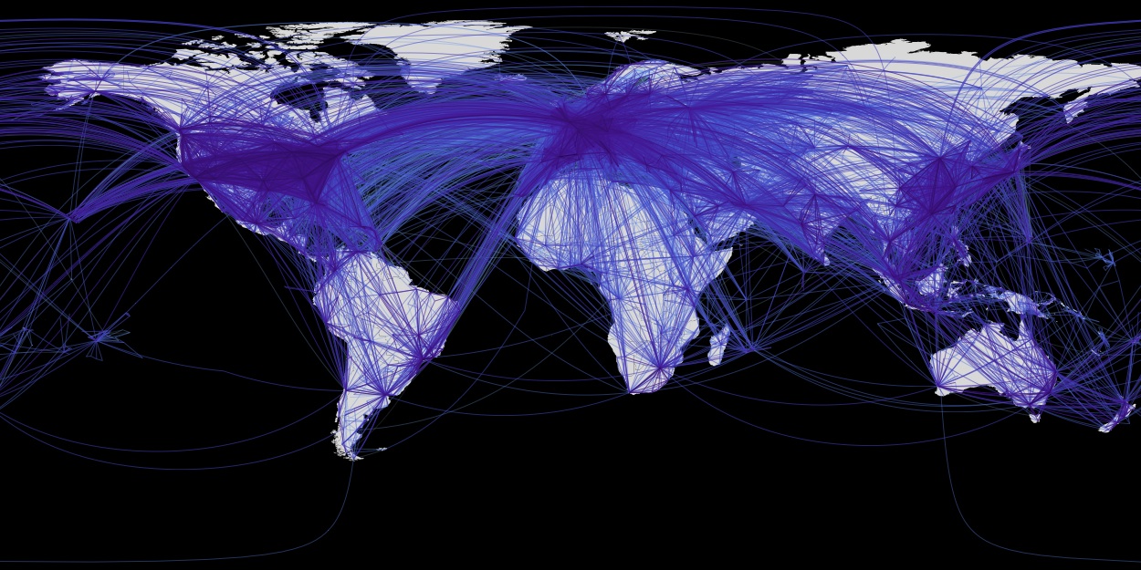
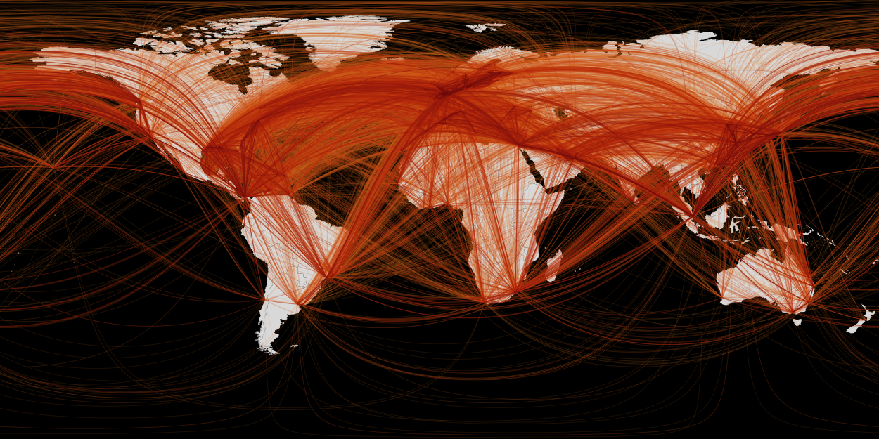
Figure 1: Global Transportation and Mobility: The top network illustrates the worldwide air-transportation network (WAN) consisting of $4,069$ airports connected by $25,453$ links that represent the number of passenger planes travelling between nodes per unit time. The saturation of the lines indicates the total flux along a route. The bottom panel depicts the global cargo-ship network (GCSN) that connects $951$ international ports along $25,819$ routes.

The WAN and GCSN are infrastructure systems on which we travel and transport commodities on a worldwide scale. Complex network theory Newman (2003); Barrat et al. (2004); Dall’Asta et al. (2006) provides the most plausible quantitative description of these systems: pairs of nodes $i$ and $j$ are connected by links with non-negative weights $w_{ij}>0$ if transport occurs directly between these nodes, and $w_{ij}=0$ if they are not directly connected. It is generally possible in transportation networks to begin at any node and locate a path to any other node, but the $w_{ij}$ measure only direct connections and quantify the magnitude of traffic between pairs of nodes. In the WAN nodes represent airports and the weight matrix could be defined as the total number of passengers per unit time, the number of passenger planes or the number of scheduled flights. In the GCSN nodes represent ports, and $w_{ij}$ could quantify the number of cargo ships or the net tonnage of cargo per unit time. For a comparative analysis we choose $w_{ij}$ to represent the number of carrier vehicles (passenger planes or cargo ships) that travel from node $j$ to $i$ per unit time. For the WAN, $w_{ij}$ is the average number of scheduled commercial flights per year between airports in the three-year period 2004–2006, as reported by OAG Worldwide Ltd. OAG Worldwide Ltd. (2007). The GCSN was established from data of world-wide ship movements provided by IHS Fairplay IHS Fairplay (2008). This information was used to reconstruct the journey of 15,415 ships travelling around the globe during 2007 Kaluza et al. (2010). The GCSN is restricted to vessels bigger than 10,000 gross tonnages which accounts for 86% of the world fleet. For both, WAN and GCSN, the resulting weight matrix $W$ is virtually symmetric, i.e. $w_{ij}\approx w_{ji}$ for all pairs $ij$. In order to guarantee strict symmetry we symmetrized the matrix according to $w_{ij}\rightarrow(w_{ij}+w_{ji})/2$. This differs from the definition that was used in  Kaluza et al. (2010), where the number of directed links was reported.

Both networks are depicted in Fig. 1.

	$N$	$L$	$\sigma$	$\phi$	$d_{\text{T}}$	$c$	$\left\langle r\right\rangle$	$C$	$\left\langle w\right\rangle$	$\left\langle F\right\rangle$	$\left\langle k\right\rangle$	$\text{CV}(w)$	$\text{CV}(F)$	$\text{CV}(k)$
WAN	$4,069$	$25,453$	$3.07\times 10^{-3}$	$29.11$	$4.16$	$0.55$	$1,109$	$5.68\times 10^{7}$	$1116.49$	$1.39\times 10^{4}$	$12.51$	$2.03$	$3.60$	$2.15$
GCSN	$951$	$25,819$	$5.72\times 10^{-2}$	$13.57$	$2.34$	$0.57$	$1,857$	$9.87\times 10^{5}$	$19.11$	$1.04\times 10^{3}$	$54.30$	$7.27$	$2.34$	$1.22$

Table 1: Network characteristics of WAN and GCSN. Number of nodes $N$, number of links $L$, network connectivity $\sigma\approx 2L/N^{2}$, network diameters $\phi$ and $d_{\text{T}},$ network clustering coefficient $c$ and network length scale $\left\langle r\right\rangle$ (in units km), total traffic $C$ (vehicles/yr.) reflect global properties of the network. The table also lists the mean link weights $\left\langle w\right\rangle$, traffic per node (flux) $\left\langle F\right\rangle$ (both in units of vehicles/yr.) and node degree $\left\langle k\right\rangle$ and corresponding coefficients of variation.

Despite their global coverage and structural similarity, these networks exhibit distinct features. The WAN comprises approximately five times as many nodes but almost the same number of links, yielding a less-densely-connected network ($\sigma_{\text{WAN}}=3.07\times 10^{-3}$ as compared to $\sigma_{\text{GCSN}}=5.72\times 10^{-2}$, see Table 1). Note that the GCSN here is restricted to large vessels Kaluza et al. (2010) and consequently the total number of seaports in the world may be an order of magnitude higher, and thus in a similar range as the WAN.

Node flux and degree are key characteristics, defined according to

$$F_{i}=\sum_{j}w_{ij}\quad\text{and}\quad k_{i}=\sum_{j}a_{ij},$$ (1)

where $a_{ij}$ are elements of the adjacency matrix, that is $a_{ij}=1$ if nodes $i$ and $j$ are connected and $a_{ij}=0$ otherwise. On average a node in the WAN dispatches $\left\langle F\right\rangle_{\text{WAN}}=1.39\times 10^{4}$ vehicles per year. The average number of cargo ships leaving a port in the GCSN is $\left\langle F\right\rangle_{\text{GCSN}}=1.03\times 10^{4}.$ Higher connectivity of the GCSN is also reflected in the mean degree, $\left\langle k\right\rangle_{\text{WAN}}=12.51$ and $\left\langle k\right\rangle_{\text{GCSN}}=54.30$.

The typical traffic per link is given by the mean link weight $\left\langle w\right\rangle$, and although in the WAN it exceeds the GCSN by two orders of magnitude, the variability reflected in the coefficient of variation is significantly higher in the GCSN. The clustering coefficient $c$ indicates the abundance of triangular motifs in the network, and in spite of the GCSN’s higher connectivity the clustering coefficient is nearly identical in both networks. This indicates that both networks can be considered sparse and saturation effects are not significant.

A typical length scale of the network can be defined by

$$\left\langle r\right\rangle=\sum_{j,i}p_{ji}r_{ji}$$ (2)

where $p_{ji}=w_{ji}/F_{j}$ and $r_{ji}$ the geographical distance between nodes $j$ and $i$. The quantity $p_{ji}$ is the relative fraction of traffic from $i$ to $j$ with respect to the entire traffic through node $i$. Thus $\left\langle r\right\rangle$ represents the mean distance traveled by a carrier in the network. According to this definition the typical length scale of the GCSN is approximately twice the size of the typical length scale of the WAN, see Table 1. Related to the geographic distance are topological distance measures defined by the connectivity of the networks. The diameter of a network can be defined as the average shortest-path length that connects a pair of nodes, $d_{\text{T}}$. For WAN and GCSN $d_{\text{T}}=4.16$ and $2.34$, respectively (in a fully connected network $d_{\text{T}}=1$).

III Universal statistics in large-scale transportation networks

A key feature that many large-scale technological networks share is their strong structural heterogeneity in terms of link and node statistics and centrality measures. These networks typically contain a small fraction of hubs characterized by strong connectivity and high centrality scores complemented by a large number of smaller nodes that connect to the hubs. Distributions of centrality measures are often scale-free Barabasi and Albert (1999); Vespignani (2009). Both the WAN and the GCSN exhibit these structural properties and, more importantly, their centrality statistics are almost identical, as is illustrated in Fig. 2, which shows the relative frequencies of link weights, node degree, and node flux.

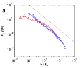
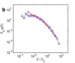
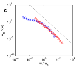
Figure 2: Statistical properties of WAN (blue) and GCSN (red): Panels a,b,c depict the probability density functions of node degree $k$, node flux $F$ and link weight $w$. Up to scaling factors these distributions exhibit very similar functional shapes. Link statistics are shown in d (link weights $w$) and e (weighted link betweenness $b$). Approximate scaling behavior is indicated by dashed lines in each panel. Scaling exponents in a and c are $\alpha=1.5$ and $\beta=2$, respectively. The abscissal scaling factors $k_{0},F_{0},w_{0}$ are given by the mean in each distribution.

Figure 2 suggests that $w$, $k$, and $F$ follow almost identical distributions (up to a scaling factor) and range across many orders of magnitude. Their surprisingly similar shape supports the claim that these networks have evolved according to similar fundamental processes. It has been pointed out Brockmann et al. (2006); Brockmann and Theis (2008); Dall’Asta et al. (2006); Barrat et al. (2005) that degree, flux, and weight approximately follow power laws. This is confirmed for $p(w)$ and $p(k)$, and we find

$$p(k)\sim k^{-\alpha}\quad\text{and}\quad p(w)\sim w^{-\beta}$$ (3)

with exponents $\alpha\approx 1.5$ and $\beta\approx 2$.

III.1 Weighted betweenness centrality of links and nodes

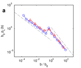
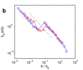
Figure 3: Structure of betweenness centrality of WAN (blue) and GCSN (red): Panels a and b depict the distributions $p(b)$ of betweenness of links and nodes, respectively. Node betweenness exhibits two distinct regimes separated by a distinct discontinuity for intermediate betweenness values. Each regime is characterized by a scaling exponent $\gamma_{1}=1.6$. Link betweenness exhibits two scaling regimes separated by a marked discontinuity as well, with two different exponents $\gamma_{2}=1.2$ ($b\ll b_{0}$) and $\gamma_{2}=2.0$ ($b\gg b_{0}$). The abscissal scaling factors $b_{0}$ are given by the mean in each distribution.

Another commonly investigated measure for link and node centrality is betweenness centrality. The betweenness $b$ of a link (or a node) is the fraction of shortest paths in the entire network of which the link (or node) is part of. Betweenness requires the definition of length of a path which in turn requires the definition of length of a link. In weighted networks a plausible choice for the effective length of a link connecting nodes $i$ and $j$ is given by the proximity $\lambda_{ij}$ defined by

$$\lambda_{ij}=\frac{\left\langle w\right\rangle}{w_{ij}}.$$ (4)

This definition accounts for the notion that strongly connected nodes are effectively more proximate than nodes that are weakly coupled. The numerator $\left\langle w\right\rangle$ sets the typical distance scale $\lambda_{0}=1/\left\langle w\right\rangle$ and $\lambda_{ij}$ is defined relative to it. Based on this effective proximity one can define the length of a path $P(i_{0},...,i_{k})$ that starts at node $i_{0}$ and terminates at node $i_{k}$ connecting a sequence of intermediate nodes $i_{n}$, $n=1,...,k-1$ along direct connections of weights $w_{i_{n}i_{n+1}}$ by summing of the proximities of each leg in the path. This integrated distance $l(i_{0},...i_{k})$ is given by the sum

$$l(i_{0},...i_{k})=\sum_{n=0}^{k-1}\lambda_{i_{n}i_{n+1}}=\sum_{n=0}^{k-1}\frac{\left\langle w\right\rangle}{w_{i_{n}i_{n+1}}}.$$ (5)

For a given pair of nodes, $i_{0}$ and $i_{k}$ many paths exists that connect these nodes along intermediate nodes $i_{n}=1,...,k-1$. Using the definition of length of a path above, the shortest path between two nodes is defined as one with minimal $l$.

$$d(i_{0},i_{k})=\min_{i_{n}=1,..k-1}l(i_{0},...,i_{k}).$$

We define the effective distance $d_{ij}$ between nodes $i$ and $j$ as this effective length of the shortest path connecting them, i.e. $d_{ij}=d(i,j)$ and denote the unique path associated with it by $P_{s}(i,j)$. Based on this definition we define the diameter $\phi$ of the network as the mean shortest-path length over the ensemble of all pairs of nodes. According to this definition the WAN’s diameter is slightly more than twice the diameter of the GCSN, see Table 1. The reasons for this will be discussed in more detail in Section V.

We computed betweenness centrality $b$ for both, links and nodes based on the set of all shortest paths $P(i,j)$. Figure 3 depicts the distributions $p(b)$ for both networks. Unlike the centrality measures of degree and flux for nodes and weights for links, the distribution of betweenness exhibits a well pronounces discontinuity in both networks. This indicates that in the WAN and GCSN links and nodes segragate into two distinct functional groups. In fact the point $b_{c}$ at which the discontinuity occurs can be employed to separate links and nodes that belong to the operational backbone of the network Grady et al. (2011). A key observation is that the distribution of betweenness in both networks is very similar: both exhibit the discontinuity and both exhibiting scaling behavior in the two betweenness regimes.

III.2 Correlations in centrality measures

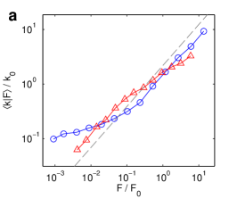
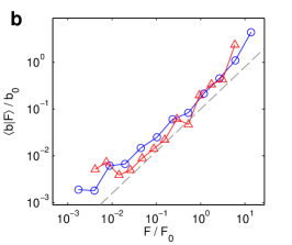
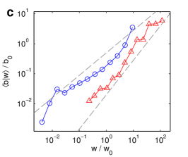
Figure 4: Correlation structure of centrality measures. a: The conditional mean degree $\left\langle k|F\right\rangle$ as a function of flux $F$. Both WAN (blue) and GCSN (red) exhibit a similar sub-linear scaling with exponent $\eta\approx 0.75$ across the entire flux range. b: Conditional mean node betweenness $\left\langle b|F\right\rangle$ as a function of $F$ is almost identical in both networks with almost linear scaling $\zeta\approx 0.9$. c: Conditional weight betweenness $\left\langle b|w\right\rangle$ as a function of $w$ exhibits different scaling in both networks. The WAN exhibits sub-linear scaling ($\xi\approx 0.75$) contrary to the GCSN for which super-linear scaling is observed ($\xi\approx 1.15$).

Degree, flux and betweenness typically exhibit positive correlations and scaling relationships with one another. For instance, recently-investigated mobility networks Barrat et al. (2005); Brockmann and Theis (2008); Kaluza et al. (2010) exhibit a sub-linear scaling relation $k\sim F^{\eta}$ with exponent $\eta\approx 0.58$ and $\eta\approx 0.7$. Figure 4 compiles scaling relationships we observe in the WAN and GCSN. To extract the scaling relationship we computed the mean of one centrality measure $x$ conditioned on a second centrality measure $y$, that is,

$$\left\langle x|y\right\rangle=\frac{\int\text{d}x\,x\,p(x,y)}{\int\text{d}x\,p(x,y)}$$ (6)

where $p(x,y)$ is the combined distribution of both. Our analysis shows that both networks exhibit a sub-linear correlation of degree with flux

$$\left\langle k|F\right\rangle\sim F^{\eta}$$ (7)

with approximately identical exponent $\eta=0.75$ for both networks and across 4 orders of magnitude of $F$. This is consistent with previous findings and the intuitive notion that node connectivity increases with traffic. A sub-linear scaling of degree with flux implies that the typical weight $\left\langle w|F\right\rangle$ of links connected to nodes of size $F$ scales according to

$$\left\langle w|F\right\rangle\sim F/\left\langle k|F\right\rangle\sim F^{1-\eta}$$ (8)

Since $\eta<1$ this implies that high flux nodes typically connect to other nodes with stronger links, as expected for transportation networks. The fact that $\eta$ is almost identical in both networks is additional evidence that similar universal mechanism are responsible for shaping the topological structure of both the WAN and GCSN. Similarly, node betweenness scales as

$$\left\langle b|F\right\rangle\sim F^{\zeta}$$ (9)

with an exponent $\zeta\approx 1$ in both networks. A linear relationship between node flux and betweenness can be explained by the heuristic argument that typical betweenness values of a node increase linearly with its degree $k$. Likewise, since shortest paths are computed based on link weights, it is reasonable to assume that node betweenness scales linearly with the typical link weight of a node and thus

$$\left\langle b|F\right\rangle\sim\left\langle k|F\right\rangle\left\langle w|F\right\rangle\sim F^{\eta}F^{1-\eta}=F$$ (10)

and hence one expects $\zeta\approx 1$ as observed. Conditional mean of link betweenness as a function of link weight $\left\langle b|w\right\rangle$ exhibit approximate scaling. Fig. 4c suggests sub-linear scaling for the WAN as opposed to super-linear scaling for the GCSN. This difference in scaling in both networks is the first marked difference that we observe in the statistics of centrality measures. Possible explanations are the differences in overall connectivity $\sigma$ in both networks (see Table 1) and that there is a statistically-significant difference in the way that weights are distributed among the nodes.

IV Network Resilience

A key question in the context of large-scale technological and infrastructural networks concerns their response to local failure and resilience to accidental, partial breakdown or anticipated attacks. Both the WAN and GCSN are subject to unpredictable, recurrent, and extreme weather conditions that lead to repetitive and regionally-localized failure that must be compensated for by re-routing traffic or re-planning schedules.

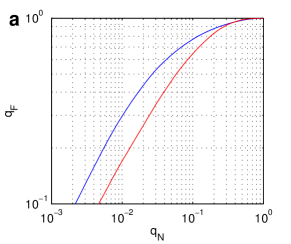
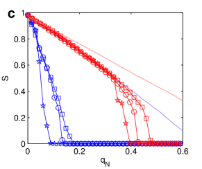
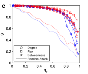
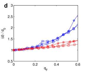
Figure 5: Resilience properties of WAN (blue) and GCSN (red) in response to random and selected node removal: a) Fraction $q_{F}$ of total traffic that is carried by a fraction $q_{N}$ of top-flux nodes. In both networks a few most central nodes carry substantial amount of traffic in the network. b) The relative size of the largest connected component of the networks as a function of the fraction $q_{N}$ of removed nodes. Nodes are removed according to the rank in terms of degree $k$ (circles), flux $F$ (squares), betweenness $b$ (stars), or randomly (no symbols). Both networks exhibit percolation thresholds under the attack protocols. Numerical values of the percolation thresholds are given in the text. c) The largest component as a function of fraction of removed traffic does not exhibit a clear percolation threshold even when almost all the traffic is removed. This indicates that the integrity of the entire network is not altered substantially even if an unrealistically large amount of traffic is reduced. d) The response to selected node removal as reflected in network inflation. The panel depicts the diameter of the network as defined by the mean shortest path between all pairs of nodes. Both networks show a substantial increase in diameter as a function of reduced traffic. The effect is more substantial in the WAN.

Random failures and targeted attacks are typically investigated using the framework of percolation theory Cohen et al. (2000, 2003). A random (failure) or selected (attack) fraction $q$ of nodes is removed from the network and structural responses of the network are investigated as a function of $q$. Important insight was gained in studies that investigated random or selected node removal in random networks Albert et al. (2000); Chen et al. (2008); Cohen et al. (2000, 2003). One of the most important findings of these studies was that scale-free networks with power-law degree distributions respond strikingly differently in scenarios that reflect random failures as opposed to selected removal of central nodes. For instance, scale-free networks are relatively immune to random removal of nodes and extremely sensitive to targeted removal of high centrality nodes. Since centrality measures such as degree, betweenness, and flux typically correlate in these networks, this effectively amounts to removal of nodes that function as hubs. One of the essential questions in this context addresses the critical fraction $q$ of removed nodes that are required to disintegrate the global connectivity of the network. This critical value is the percolation threshold $q_{c}$: for $q<q_{c}$ the size of the giant component (the largest subset of nodes that are connected by paths) is typically the size of the entire network. Beyond the percolation threshold ($q>q_{c}$) the networks falls apart into a family of disconnected, fragmented sub-networks.

The resilience properties of the WAN and GCSN to sequential node removal are depicted in Fig. 5. For each centrality measure (degree, betweenness, and flux), we remove fractions $q$ of nodes according to their rank with respect to $k$, $b$, and $F$, respectively. We compare two different removal protocols. Since both networks are strongly inhomogeneous, removing a fraction of nodes is not equivalent to removing a fraction of traffic (see Fig. 5a). For example $1\%$ of the most connected nodes account for $29.7\%$ of the entire traffic in the WAN and $17.6\%$ in the GCSN, and removal of $10\%$ of nodes with highest flux is equivalent to reducing the total traffic in the WAN by $76.9\%$ and in the GCSN by $64.5\%$. Because of this pronounced nonlinear relationship, we compare resilience of the network as a function of the fraction of removed nodes $q_{N}$ as well as the fraction of removed traffic $q_{F}$.

Figure 5b depicts the relative size of the giant component $S$ as a function of $q_{N}$. Both networks are resilient to random failures (we find that the giant component decreases lineary with the fraction of nodes removed, i.e. $S\approx 1-q_{N}$), although the WAN is taking some excess damage from random failures. Furthermore, we observe a percolation threshold for the targeted attacks in both networks. The WAN exhibits a percolation threshold at $q_{N}^{c}=13.8\%,\,17.2\%$ and $9.4\%$, for node removal according to degree, flux and betweenness. The thresholds are significantly larger for the GCSN at $q_{N}^{c}=44.3\%,49.0\%$ and $39.5\%$. In each network the threshold depends only weakly on the choice of centrality measure because of the strong correlation among different centrality measures. Note however that both networks are most susceptible to removal according to betweenness rank, followed by degree and node flux. The overall higher threshold in the GCSN is caused by the greater connectivity $\sigma$ and mean degree $\left\langle k\right\rangle$ of the network (see Table 1).

Figure 5c depicts $S$ as a function of $q_{F}.$ The random failures appear to be more effective here because they remove more nodes for a given fraction of removed traffic than the targeted attacks, since not only high-centrality nodes are selected. However, due to the strong nonlinear relationship between $q_{N}$ and $q_{F}$ it is evident that both networks are strongly resilient to targeted attacks. Even substantial traffic reduction has virtually no impact on the relative size of the giant component, for instance when 50% of the entire traffic is reduced in both networks, the giant component is still larger than $90\%$ of the original network and no percolation threshold is observed in the range up to $80\%$ of traffic reduction. These traffic reductions are unrealistic when compared to actual perturbations of real transportation networks. Percolation thresholds are therefore never reached under realistic conditions. Another approach that has been applied in unweighted networks Albert et al. (2000) is based on the diameter of the network and its response to network disruption. Typically when high-centrality nodes are removed from the network, the diameter of the network increases as the shortest paths connecting two arbitrary nodes lengthen due to the increasing lack of hubs that can serve as connecting junctions. Figure 5d shows that this inflation of the network in response to node removal is observed in both networks. This effect is relatively independent of the choice of centrality measure used in the removal protocol. Furthermore, the GCSN is more robust to node reduction, which we believe to be a consequence of the high connectivity of the network.

Both percolation analysis and network inflation have only limited applicability in real world scenarios. Since real world network disruptions never reach the percolation threshold and network inflation only address global structural changes in network properties, a more refined quantity is needed that can determine the response to external perturbations below the percolation threshold and on a node by node basis. In section IV we propose a technique to quantify network resilience that permits the study of network pertubations in a more refined framework and well below the percolation threshold based on shortest-path trees. The key idea behind this technique is the ability to quantify the effect of network disruptions for each node and perform network-wide statistics of the impact of external pertubations or network disruptions.

V Network shortest-path trees

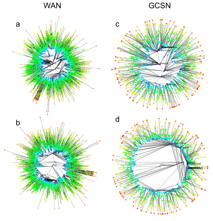
Figure 6: Shortest-path tree structures and effective distances in WAN and GCSN. Left: The panels depict the shortest-path trees of airports ATL (Atlanta) and PVG (Shanghai). The radial distance of the remaining airports with respect to these root nodes represent the logarithm of the shortest-path distance to the reference node. Right: The panels depict the GCSN shortest-path tree for ports Wilhelmshaven, Germany and Shanghai. Note that the overall structure of both representations is different, yet both networks share the feature of circular arrangement according to node flux, encoded by color (blue represents large flux nodes and orange small node flux). Note that irrespective of the chosen root node, the closest nodes in terms of effective distance are always high flux nodes and small flux nodes are always peripheral in this representation.

Global properties of strongly heterogeneous, multi-scale networks, such as connectivity, clustering coefficient, and diameter, as well as statistical distributions of centrality measures, provide important insight and may serve as quantitative classifiers for networks. However, they cannot resolve properties and structures on a local scale. On the other hand, local measures such as a node’s individual degree, betweenness centrality, or mean link weight of its connections provide local information only and cannot capture global properties. Transportation networks exhibit important structure on intermediate scales, so it is vital to understand structural properties that are neither local nor global in these networks. One way to approach this is to analyse and investigate the structure of the entire network from the perspective of a chosen node. Clearly, geographic distance is an important parameter in this context as operation costs typically scale with geographic distance. However, in complex multi-scale transportation networks such as the WAN and the GCSN, geographic distance is rarely a good indicator of the effective distance of connected nodes. High-flux hubs in each network are typically connected by strong traffic bonds even across very large geographic distances while smaller-flux nodes can be connected by weak links although they may be geographically close. A spatial representation as depicted in Fig. 1 is therefore a misleading way to convey effective distances in these networks.

An alternative representation can be obtained based on the notion of proximity defined by Eq. (4) and effective shortest paths, Eq. (5). Based on this notion we compute the shortest paths of a chosen root node $i$ to all other nodes $j$. The collection of links contributing to these paths form a shortest-path tree $\mathbf{T}_{i}$ rooted at $i$. Spatial representations of such trees are depicted in Fig. 6 for each network and two different root nodes. The radial distance in these figures represents the effective, shortest-path distance $d_{ji}$. The lines represent the connections of $\mathbf{T}_{i}$. Note that, although the trees differ in both networks and for different root nodes, high-centrality nodes tend to exhibit the smallest effective (shortest-path) distance to the root node. Note also that the geometry of the networks exhibits significant structural differences in both networks: In the WAN the spatial distribution in the new representation is less regular and the scatter in effective distance is larger than in the GCSN where nodes reside in a well defined annular region.

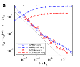
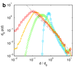
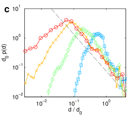
Figure 7: Shortest-path distance statistics. a: Conditional mean shortest path (Eq. 11) as a function of node flux as well as the conditional coefficient of variation in shortest paths. Both networks exhibit a universal decrease of expected shortest path with node flux determined by an exponent $\tau\approx 0.75$, see Eq. 12. The variability of shortest-path distance increases in both networks, but less markedly in the GCSN than in the WAN. b: The conditional distributions of shortest paths for four subtypes of root nodes (WAN) ranked according to flux, where red markers denote high flux and light blue denote low flux. c: Same as in b for the GCSN. The dashed grey lines indicate a scaling relation with exponent $\theta\approx 1.5$ (WAN) or $\theta\approx 1.25$ (GCSN).

In order to understand these qualitative differences and similarities we investigate the distribution of the shortest-path distances conditioned on the type of root node. The results of this analysis are depicted in Fig. 7. Conditioned on the flux of the root node, we compute the distribution of shortest-path distance, that is, $p(d|F).$ Based on this distribution we determine the expected distance of the network from a node with specified flux as

$$\mu_{d}(F)=\left\langle d|F\right\rangle$$ (11)

as well as the conditional coefficient of variation:

$$\text{cv}_{d}(F)=\frac{\sqrt{\left\langle d^{2}|F\right\rangle-\left\langle d|F\right\rangle^{2}}}{\left\langle d|F\right\rangle}$$

The quantity $\mu_{d}(F)$ measures the typical distance from a root node with flux $F$ to the rest of the network. The coefficient of variation measures the statistical variability in $d$. Figure 7 depicts both quantities for the WAN and GCSN. Note that $\mu_{d}(F)$ behaves identically for both networks and can described by

$$\mu_{d}(F)-\mu_{d}(\infty)\sim(F/F_{0})^{-\tau}$$ (12)

with $\tau\approx 0.75$. Note that this relation indicates the existance of a lower limit to the typical effective distance for increasing node flux $\mu_{d}(\infty)>0$ which implies that even extremely large hubs exhibit a least distance to the rest of the network. Eq. (12) implies that mean effective distance decreases in a systematic way with node centrality and according to the same relation in both networks. However, the coefficient of variation increases monotonically with $F$, which implies that the variability in effective distance increases with the centrality of the root node. This can also be observed in Fig 7b and c, which depicts the entire distribution $p(d|F)$ for four categories of root nodes of different centrality. For most central nodes $p(d|F)$ increases steeply for small values of $d$ and exhibits an algebraic decay for large distance. As $F$ decreases, $p(d|F)$ attains a sharper peak as small distances disappear from the distribution. This qualitative behavior is observed in both networks. The asymptotic behavior for large effective distances is approximately

$$p(d|F)\sim d^{-\theta}$$

with $\theta\approx 1.5$ for the WAN and $\theta\approx 1.25$ for the GCSN.

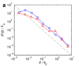
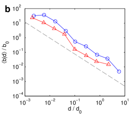
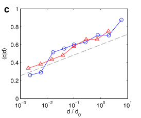
Figure 8: Correlation analysis of shortest paths and centrality measures (a) flux, (b) weighted node betweenness for WAN (blue) and GCSN (red). Both networks exhibit almost identical scaling relations. The scaling exponents are given by $\omega_{F}=1.5$, $\omega_{b}=1.1$. c: the local clustering coefficient $c$ as a function of effective distance $d$ increases logarithmically.

A characteristic property of the network representation in Fig. 6 is that regardless of the properties of the root node, the rest of the nodes tend to sort in concentric circles (effective distances) according to centrality measures. A key question is then how effective distance correlates with centrality measures. If there is a strong correlation between effective distance and node centrality measures, this implies that centrality measures dominate the placement of a node in a network.

In order to determine the relationship between effective distance and centrality measures, we selected $2.5\%$ of the most central nodes, according to degree, flux and betweenness and collected them in a subset of nodes $\Omega$. The fraction of nodes in this set represents $5\%$ of the entire network. The remaining $95\%$ of the nodes are denoted by $\bar{\Omega}$. Based on this subset we determine the distribution $p(x,d|\Omega)$, the probability of finding a node in $\bar{\Omega}$ with centrality measure $x$ (degree, flux, betweenness) and effective distance $d$ to the root nodes in $\Omega$. From this we computed the conditional mean

$$\left\langle x|d\right\rangle=\int x\,p(x|d,\Omega)=\int x\,p(x,d|\Omega)/p(d|\Omega),$$ (13)

Figure 8 depicts $\left\langle F|d\right\rangle$ and $\left\langle b|d\right\rangle$ for both networks. Despite their difference, WAN and GCSN exhibit almost identical scaling relations

$$\left\langle F|d,\Omega\right\rangle\sim d^{-\omega_{F}}\quad\text{and}\quad\left\langle b|d,\Omega\right\rangle\sim d^{-\omega_{b}}$$ (14)

with $\omega_{F}\approx 1.5$ and $\omega_{b}\approx 1.1$, consistent with the intuitive notion that centrality decreases with increasing effective distance from central root nodes. Figure 8 also shows that the local clustering coefficient as a function of $d$ approximately scales according to

$$\left\langle c|d,\Omega\right\rangle\sim\log(d/d_{0}).$$ (15)

The logarithmic increase of the clustering coefficient implies that in their peripheral regions the WAN and GCSN become less tree-like. A plausible explanation is that low-centrality nodes that are connected to the root nodes in $\Omega$ do not exhibit large fractions of connections among one another, which indicates that high-centrality root nodes function as “feed-in” hubs to low centrality nodes.

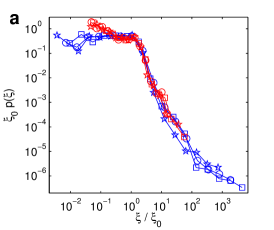
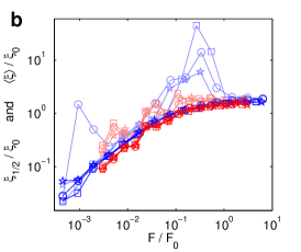
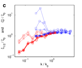
Figure 9: The distribution of impact in response to the removal of central nodes of the system as determined by degree (circles), flux (squares), and betweenness (stars) in the WAN (blue) and GCSN (red). a: $p(\xi)$ is the probability distribution of impact factors computed for each node in response to the various attacks. Note that apart from a scaling factor the distribution of impact is identical in all three attack scenarios and both networks. The impact factor $\xi$ ranges over many orders of magnitude. b: Universal behavior is also observed in the dependence of impact factor as a function of node flux $F$. The y-axis measures the normalized median impact ($\xi_{1/2}/\xi_{0}$, solid lines) and normalized mean impact ($\left\langle\xi\right\rangle/\xi_{0}$, faint lines). c: The dependence of impact factor on node degree.

V.1 Resilience and shortest paths

The concept of shortest-path trees can also give insight into the networks’ resilience properties discussed in section IV. In response to removal of a fraction $q_{N}$ of most central nodes or the equivalent fraction of traffic $q_{F}$ in the entire network, we can compute the impact by investigating the change of shortest-path trees $\mathbf{T}_{i}$ for each root node $i$, that is, we can quantify the impact of the network disruption from the perspective of every node. To this end we define a node’s impact factor as

$$\xi_{i}=\frac{\Delta\bar{d}_{i}}{\bar{d}_{i}}$$ (16)

where $\bar{d}_{i}$ is the median shortest-path distance from reference node $i$ to all other nodes $j$, and $\Delta\bar{d}_{i}$ the change of this median in response to the network disruption. This impact factor is different for every node and the distribution $p(\xi)$ gives insight into the variability of how individual nodes are affected by the network disruption Woolley Meza et al. (2011). Figure 9a illustrates $p(\xi)$ for scenarios in which the entire traffic was reduced by $30\%$ through the removal of high-centrality nodes. The distribution $p(\xi)$ is independent of the measure of centrality and also identical in both networks. Below a typical impact of $\xi_{0}$ the distribution of impact factors $p(\xi)$ is uniform and for $\xi>\xi_{0}$ it decreases slowly, ranging over many orders of magnitude. A question that immediately arises is what nodes in the network experience the largest impact. Figures 9b/c depict the mean $\left\langle\xi\right\rangle$ and median $\xi_{1/2}$ conditioned on the flux $F$ and degree $k$. Both the WAN and GCSN exhibit the same dependence, with increasing centrality, the median impact increases monotonically and reaches the typical asymptotic value $\xi_{0}.$ However, the mean $\left\langle\xi\right\rangle$ as a function of $F$ exhibits strong fluctuations for intermediate ranges of $F$. The explanation for this phenomenon is that the relative impact for low centrality nodes is small because $\bar{d}$ in the unperturbed network is very large. Nodes of intermediate centrality are affected strongly because their mean effective distance to the network $\bar{d}$ is of intermediate size as they primarily connect to hubs in the network by strong links. When the hubs are removed from the network, these nodes experience a strong increase in impact as $\Delta\bar{d}$ is increased substantially. A similar effect is seen in the behavior of $\left\langle\xi\right\rangle$ as a function of degree $k$.

VI Discussion

The comparative analysis of the worldwide air-transportation network and the global cargoship network presented here is a first step towards a better understanding of the organizational structure, the evolution and management of large scale infrastructural networks in general. The statistical analysis of node and link centrality measures and their correlations revealed a suprising degree of similarity of both networks despite their different purpose, scale and connectivity. We believe that this is strong evidence for common underlying principles that govern the growth and evolution of infrastructural networks. This is also supported by the variety of simple algebraic scaling relations that we extracted from both networks.

Our analysis revealed an unusual discontinuity in the distribution of both link and node betweenness. This suggests that strongly heterogeneous transportation and mobility networks exhibit a natural functional separation of links and nodes into two distinct groups. Interestingly, this discontinuity is localized at the same relative betweenness value and has approximately the same magnitude in both networks. We conclude that this natural separation into different classes of nodes and links might well be a universal feature of these transportation networks as well and could be a starting point for further investigations along these lines.

The analysis of network resilience showed that because of their dense connectivity, both networks cannot be investigated by conventional analysis techniques such as percolation theory or network diameter inflation. The percolation threshold for both networks lies well beyond any realistic network pertubations. The alternative approach based on effective distance, shortest paths, and shortest-path trees allows a better, more intuitive representation of networks and resilience analysis, taking into account the fact that nodes that are connected by strong traffic are effectively closer than nodes that are connected by weak links and investigating network pertubations from the viewpoint of chosen reference nodes. Furthermore, the shortest-path-tree representation revealed an interesting correlation of effective shortest path distance and node centrality measures such as flux, degree, and betweenness and an interesting symmetry in both networks: On average, any node in the network is closest to the subset of nodes with high centrality. This has fundamental implications for spreading phenomena on these types of networks. Whereas global disease dynamics, for example, is characterized by highly complex spatio-temporal patterns when visualized in conventional geographical coordinates, we expect these patterns become simpler and thus better understood when shortest-path-tree representations are employed. Since the shortest-path-tree representations are structurally similar in both networks one might expect a strong dynamic similarity of otherwise unrelated spreading phenomena that occur in these networks, for example the global spread of emergent human infectious diseases on the worldwide air-transportation network and human mediated bioinvasion processes on the global cargoship network. We conclude that our results can serve as a starting point for both the development of theories for the evolution of large scale transportation networks and dynamical processes that evolve on them.