Dissipation-induced pure Gaussian state

Abstract

This paper provides some necessary and sufficient conditions for a general Markovian Gaussian master equation to have a unique pure steady state. The conditions are described by simple matrix equations, thus the so-called environment engineering problem for pure Gaussian state preparation can be straightforwardly dealt with in the linear algebraic framework. In fact, based on one of those conditions, for an arbitrary given pure Gaussian state, we obtain a complete parameterization of the Gaussian master equation having that state as a unique steady state; this leads to a systematic procedure for engineering a desired dissipative system. We demonstrate some examples including Gaussian cluster states.

I Introduction

Preparing a desired pure state, particularly under influence of dissipation, is clearly a most important subject in quantum information technologies. To tackle this problem, other than some well-acknowledged strategies such as quantum error correction, recently we have a totally different method that rather utilizes dissipation Poyatos ; Cirac1 ; Kraus ; Kraus_nature ; TicozziViola2008 ; Ficek2009 ; TicozziViola2011 ; VerstraeteNaturePhys ; Vollbrecht ; Schirmer ; Cirac2 ; Polzik ; Yamamoto . The basic idea is to engineer a dissipative system so that the system state $\hat{\rho}(t)$ governed by the corresponding Markovian master equation

$$\frac{d\hat{\rho}}{dt}=-i[\hat{H},\hat{\rho}]+\sum_{k=1}^{m}\Big{(}\hat{L}_{k}\hat{\rho}\hat{L}_{k}^{\dagger}-\frac{1}{2}\hat{L}_{k}^{\dagger}\hat{L}_{k}\hat{\rho}-\frac{1}{2}\hat{\rho}\hat{L}_{k}^{\dagger}\hat{L}_{k}\Big{)}$$ (1)

must evolve towards a desired pure state: $\hat{\rho}(t)\rightarrow|{\phi}\rangle\langle{\phi}|$ as $t\rightarrow\infty$. Here, $\hat{H}$ is the system Hamiltonian and $\hat{L}_{k}$ $(k=1,\ldots,m)$ is the dissipative channel that represents the coupling between the system and the $k$-th environment mode. The main advantage of this environment engineering approach is that the dissipation-induced state $|{\phi}\rangle$ is robust against any perturbation and thus may serve as a desired state, e.g., an entangled state for quantum computation VerstraeteNaturePhys and quantum repeater Vollbrecht . Therefore, a complete characterization of the master equation having a unique pure steady state should be of great use, and actually in the finite-dimensional case it was given by Kraus et al. Kraus . In particular, they showed that some useful pure states including cluster states can be prepared by quasi-local dissipative process, i.e., dissipative channels that act only on a small number of subsystems.

In this research direction the infinite-dimensional counterpart of the above-mentioned state preparation method should be explored. In particular, Gaussian states constitute a wide and important class of quantum states, which serve as the basis for various continuous-variable (CV) quantum information processing Braunstein2005 ; Furusawa2011 . The contribution of this paper is to provide some necessary and sufficient conditions for the master equation (1) to have a unique pure steady state, when $\hat{H}$ and $\hat{L}_{k}$ are of general form for $\hat{\rho}(t)$ to be Gaussian for all $t$. The conditions are described by simple matrix equations, thus they can be properly applied to the above-mentioned environment engineering problem for pure Gaussian state preparation. Actually, one of those conditions enables us to obtain a complete parameterization of the Gaussian master equation that uniquely has a pure steady state. This leads to a systematic procedure for constructing a dissipative system deterministically yielding a desired pure Gaussian state. We provide some examples of dissipation-induced states including the so-called Gaussian cluster states Zhang2006 ; vanLoock2007 ; Menicucci2011 , which are known as essential resources for the CV one-way quantum computing Menicucci2006 , with focusing on how they can actually be prepared by quasi-local dissipative process.

II Gaussian dissipative systems

We here provide the phase space representation of the general Gaussian dissipative system with $n$-degrees of freedom, which is subjected to the master equation (1). Let $(\hat{q}_{i},~{}\hat{p}_{i})$ be the canonical conjugate pair of the $i$-th subsystem. It then follows from the canonical commutation relation $[\hat{q}_{i},~{}\hat{p}_{j}]=i\delta_{ij}$ that the vector of system variables $\hat{x}:=(\hat{q}_{1},\ldots,\hat{q}_{n},\hat{p}_{1},\ldots,\hat{p}_{n})^{\top}$ satisfies

$$\hat{x}\hat{x}^{\top}-(\hat{x}\hat{x}^{\top})^{\top}=i\Sigma,~{}~{}\Sigma=\left(\begin{array}[]{cc}0&I_{n}\\ -I_{n}&0\end{array}\right),$$

where $I_{n}$ denotes the $n\times n$ identity matrix and $\top$ the matrix transpose. A Gaussian state is completely characterized by only the mean vector $\langle{\hat{x}}\rangle$ and the (symmetrized) covariance matrix $V=\langle{\Delta\hat{x}\Delta\hat{x}^{\top}+(\Delta\hat{x}\Delta\hat{x}^{\top})^{\top}}\rangle/2,~{}\Delta\hat{x}=\hat{x}-\langle{\hat{x}}\rangle$. Here the mean $\langle{\hat{X}}\rangle={\rm Tr}\hskip 1.9919pt(\hat{X}\hat{\rho})$, with $\hat{\rho}$ the corresponding Gaussian density operator, is taken elementwise; e.g., $\langle{\hat{x}}\rangle=(\langle{\hat{q}_{1}}\rangle,\ldots,\langle{\hat{p}_{n}}\rangle)^{\top}$. The uncertainty relation is represented by the matrix inequality $V+i\Sigma/2\geq 0$, thus $V>0$ StefanoLloyd . Note also that the purity of a Gaussian state is simply given by $P={\rm Tr}\hskip 1.9919pt(\hat{\rho}^{2})=1/\sqrt{2^{2n}{\rm det}(V)}$. Now consider Eq. (1) with $\hat{H}$ and $\hat{L}_{k}$ given by

$$\hat{H}=\frac{1}{2}\hat{x}^{\top}G\hat{x},~{}~{}\hat{L}_{k}=c_{k}^{\top}\hat{x},$$

where $G=G^{\top}\in\textbf{R}^{2n\times 2n}$ and $c_{k}\in\textbf{C}^{2n}$ are the parameter matrix and vector specifying the dissipative system. Then, the time-evolution of $\langle{\hat{x}}\rangle$ and $V$ read

$$\frac{d\langle{\hat{x}}\rangle}{dt}=A\langle{\hat{x}}\rangle,~{}~{}\frac{dV}{dt}=AV+VA^{\top}+D,$$ (3)

where $A=\Sigma[G+\Im(C^{\dagger}C)]$ and $D=\Sigma\Re(C^{\dagger}C)\Sigma^{\top}$ with $C=(c_{1},\ldots,c_{m})^{\top}\in\textbf{C}^{m\times 2n}$ ($\Re$ and $\Im$ denote the real and imaginary parts, respectively). If $\hat{\rho}(0)$ is Gaussian, then $\hat{\rho}(t)$ is always Gaussian with mean $\langle{\hat{x}(t)}\rangle$ and covariance matrix $V(t)$. See Wiseman for detailed description.

Now suppose that $A$ is Hurwitz; i.e., all the eigenvalues of $A$ have negative real parts. This is equivalent to that the system has a unique steady state; it is Gaussian with mean $\langle{\hat{x}(\infty)}\rangle=0$ and covariance matrix $V_{s}$ that is a unique solution to the following matrix equation:

$$AV_{s}+V_{s}A^{\top}+D=0.$$ (4)

Note that $V_{s}$ can be explicitly represented as

$$V_{s}=\int_{0}^{\infty}e^{At}De^{A^{\top}t}dt.$$ (5)

The purpose of this paper is, as mentioned before, to fully characterize a Gaussian master equation that has a unique pure steady state, and this is now expressed in terms of Eq. (5) by $2^{2n}{\rm det}(V_{s})=1$. However, clearly this is not useful. In the next section we give a much simpler and explicit version of such a characterization.

III The dissipation-induced pure Gaussian states

III.1 Pure steady state condition

Here we address our first main result:

Theorem 1: Suppose that Eq. (4) has a unique solution $V_{s}$. Then the following three conditions are equivalent:

• The system has a unique pure steady state with covariance matrix $V_{s}$.

• $V_{s}$ satisfies the following matrix equations:

  $$\Big{(}V_{s}+\frac{i}{2}\Sigma\Big{)}C^{\top}=0,$$ (6)

  $$\Sigma GV_{s}+V_{s}G\Sigma^{\top}=0.$$ (7)

• The following matrix equation holds:

  $$K\Sigma C^{\top}=0,$$ (8)

  where $K\in{\bf C}^{2nm\times 2n}$ is defined by

  $$K=(C^{\top},\ G\Sigma^{\top}C^{\top},\cdots,(G\Sigma^{\top})^{2n-1}C^{\top})^{\top}.$$ (9)

Furthermore, when the above equivalent conditions are satisfied, $V_{s}$ is represented by

$$V_{s}=\frac{1}{2}\Sigma^{\top}\Im(K^{\dagger}K)[\Re(K^{\dagger}K)]^{-1}.$$ (10)

To prove this theorem we need the following lemma.

Lemma 1: Suppose that Eq. (4) has a unique solution. Then ${\rm rank}(\bar{K}^{\top})=2n$, where

$$\bar{K}=(\bar{C}^{\top},~{}G\Sigma^{\top}\bar{C}^{\top},\ldots,(G\Sigma^{\top})^{2n-1}\bar{C}^{\top})^{\top}\in{\bf R}^{4nm\times 2n}$$

with $\bar{C}=(\Re(C)^{\top},\Im(C)^{\top})^{\top}\in{\bf R}^{2m\times 2n}$.

Proof of Lemma 1: From the assumption, Eq. (4) has a unique solution (5). Suppose there exists a vector $\xi\in{\bf R}^{2n}$ such that $\bar{K}\xi=0$. Then, noting that $A$ and $D$ are written by $A=\Sigma[G+\bar{C}^{\top}\Sigma\bar{C}]$ and $D=\Sigma\bar{C}^{\top}\bar{C}\Sigma^{\top}$, we have $\xi^{\top}\Sigma^{\top}V_{s}\Sigma\xi=\int_{0}^{\infty}\|\bar{C}\Sigma^{\top}e^{A^{\top}t}\Sigma\xi\|^{2}dt=0$, and this is contradiction to $V_{s}>0$. Thus ${\rm rank}(\bar{K}^{\top})=2n$. $\blacksquare$

Proof of Theorem 1: The proof is divided into four steps.

1. (i) $\Rightarrow$ (ii). From the Williamson theorem Williamson a covariance matrix $V$ corresponding to a pure state is expressed by $V=SS^{\top}/2$ with $S$ a symplectic matrix Simon . Thus substituting $V_{s}=SS^{\top}/2$ for Eq. (4), multiplying it by $S^{-1}$ from the left and by $S^{-\top}$ from the right, and finally using this equation twice to erase $G$, we have

$$(C_{r}^{\prime\top}-\Sigma C_{i}^{\prime\top})(C_{r}^{\prime\top}-\Sigma C_{i}^{\prime\top})^{\top}$$

$$\mbox{}+(C_{i}^{\prime\top}+\Sigma C_{r}^{\prime\top})(C_{i}^{\prime\top}+\Sigma C_{r}^{\prime\top})^{\top}=0,$$

where $C_{r}^{\prime}=\Re(C)S$ and $C_{i}^{\prime}=\Im(C)S$. Note $S\Sigma S^{\top}=\Sigma$. Thus $C_{r}^{\prime\top}-\Sigma C_{i}^{\prime\top}=C_{i}^{\prime\top}+\Sigma C_{r}^{\prime\top}=0$, which immediately leads to $V_{s}\Re(C)^{\top}=\Sigma\Im(C)^{\top}/2$ and $V_{s}\Im(C)^{\top}=-\Sigma\Re(C)^{\top}/2$. From these equations we obtain Eq. (6). Combining this with Eq. (4) yields Eq. (7).

2. (ii) $\Rightarrow$ (iii). Multiplying Eq. (6) by $\Sigma G$ from the left and using Eq. (7), we get $(V_{s}+i\Sigma/2)G\Sigma^{\top}C^{\top}=0$. Repeating this manipulation yields

$$(V_{s}+i\Sigma/2)K^{\top}=0,$$ (11)

with $K$ defined in Eq. (9). This readily leads to $K(V_{s}\pm i\Sigma/2)K^{\top}=0$, thus $K\Sigma K^{\top}=0$. The Cayley-Hamilton theorem implies Eq. (8).

3. Derivation of Eq. (10). Define the $4nm\times 2n$ matrix $K^{\prime}=(\Re(K^{\top}),~{}\Im(K^{\top}))^{\top}$, then the real and imaginary parts of Eq. (11) are summarized in a single equation as

$$\Sigma V_{s}K^{\prime\top}=K^{\prime\top}\Sigma/2.$$

Now, from the assumption, we can use Lemma 1 and find ${\rm rank}(K^{\prime\top})={\rm rank}(\bar{K}^{\top})=2n$. Then multiplying the above equation by $K^{\prime}(K^{\prime\top}K^{\prime})^{-1}$ (the generalized inverse matrix of $K^{\prime\top}$) from the right, we have

$$\Sigma V_{s}=(K_{r}^{\top}K_{i}-K_{i}^{\top}K_{r})(K_{r}^{\top}K_{r}+K_{i}^{\top}K_{i})^{-1}/2,$$

where $K_{r}=\Re(K)$ and $K_{i}=\Im(K)$. This is just Eq. (10).

Now let us verify that Eq. (10) is symmetric. Noting that Eq. (8) is equivalent to $K\Sigma K^{\top}=0$, we have

$$\left(\begin{array}[]{c}K\\ K^{*}\end{array}\right)\Sigma(K^{\top},~{}-K^{\dagger})=\left(\begin{array}[]{c}K\\ -K^{*}\end{array}\right)\Sigma^{\top}(K^{\top},~{}K^{\dagger}).$$ (12)

Then multiplying this equation by $(K^{\dagger},~{}K^{\top})$ from the left and by $(K^{\dagger},~{}K^{\top})^{\top}$ from the right, we obtain

$$\Re(K^{\dagger}K)\Sigma\Im(K^{\dagger}K)=-\Im(K^{\dagger}K)\Sigma^{\top}\Re(K^{\dagger}K),$$

thus $V_{s}=V_{s}^{\top}$.

4. (iii) $\Rightarrow$ (i). First, to show that the state is pure, we use the fact Wolf that, for a pure Gaussian state, the corresponding covariance matrix $V$ satisfies

$$\Sigma V\Sigma V=-I/4.$$ (13)

Now multiply Eq. (12) by $(K^{\dagger},~{}K^{\top})$ from the left and by $(K^{\dagger},~{}-K^{\top})^{\top}$ from the right, then we have

$$\Re(K^{\dagger}K)\Sigma\Re(K^{\dagger}K)=\Im(K^{\dagger}K)\Sigma^{\top}\Im(K^{\dagger}K).$$

This equation readily implies that $V_{s}$ given by Eq. (10) satisfies Eq. (13), hence the corresponding state is pure.

Next, let us show that Eq. (10) satisfies Eq. (4). Note that Eq. (10) is rewritten as $V_{s}\Re(K^{\dagger}K)=-\Sigma\Im(K^{\dagger}K)/2$. Also from Eq. (13) we have $V_{s}\Im(K^{\dagger}K)=\Sigma\Re(K^{\dagger}K)/2$. These two equations yield

$$(V_{s}-i\Sigma/2)K^{\dagger}K=0,$$

which is equivalent to $(V_{s}-i\Sigma/2)K^{\dagger}=0$, thus Eq. (11). This implies that Eq. (6) holds. Moreover, Eq. (11) leads to $(V_{s}G\Sigma^{\top}+i\Sigma G\Sigma^{\top}/2)K^{\top}=0$ and $(\Sigma GV_{s}+i\Sigma G\Sigma/2)K^{\top}=0$; from these equations we have $(\Sigma GV_{s}+V_{s}G\Sigma^{\top})K^{\top}=0$, and as now $\Sigma GV_{s}+V_{s}G\Sigma^{\top}$ is real and ${\rm rank}(K^{\prime\top})=2n$, we obtain Eq. (7). As a result, $V_{s}$ satisfies Eqs. (6) and (7), but these two equations correspond to a specific decomposition of Eq. (4). That is, $V_{s}$ is the solution to Eq. (4). $\blacksquare$

We give an interpretation of Theorem 1. Let $\hat{\rho}_{s}$ be the pure density operator corresponding to the covariance matrix $V_{s}$. Then Eqs. (6) and (7) are equivalent to

$$2\hat{L}_{k}\hat{\rho}_{s}\hat{L}_{k}^{\dagger}-\hat{L}_{k}^{\dagger}\hat{L}_{k}\hat{\rho}_{s}-\hat{\rho}_{s}\hat{L}_{k}^{\dagger}\hat{L}_{k}=0~{}~{}\forall k,~{}~{}~{}~{}[\hat{H},\hat{\rho}_{s}]=0,$$ (14)

respectively. The former condition is further equivalent to that $\hat{L}_{k}|{\phi_{s}}\rangle$ is parallel to $|{\phi_{s}}\rangle$ for all $k$, where $\hat{\rho}_{s}=|{\phi_{s}}\rangle\langle{\phi_{s}}|$. This means that $\hat{\rho}_{s}$ is the so-called dark state; that is, Eqs. (6) and (7) are the phase space representation of the condition for the state to be dark. Moreover, the uniqueness of $\hat{\rho}_{s}$ allows us to erase itself in Eq. (14) and obtain a single equation with respect to $\hat{H}$ and $\hat{L}_{k}$. The phase space representation of this equation is no more than Eq. (8). It should be maintained that $\hat{\rho}_{s}$ is explicitly represented in a directly computable form (10).

Next let us discuss how to use Theorem 1, particularly for the purpose of environment engineering. First, note that Eq. (8) depends only on the system matrices $G$ and $C$; thus the condition (iii) should be applied, for a given specific system configuration, to find the system parameters such that the corresponding master equation has a unique pure steady state. On the other hand, the condition (ii) explicitly contains $V_{s}$; this means that we can characterize the structure of a dissipative system such that a desired pure state with covariance matrix $V_{s}$ is generated by that dissipative process. Later we provide a modification of the condition (ii) that can be more suitably used to find such a dissipative system.

III.2 Examples

We here give two examples to explain how the theorem is used.

Example 1: Single OPO. Let us first study an ideal optical parametric oscillator (OPO), which couples with a vacuum field through one of the end-mirrors. The Hamiltonian is described in terms of the annihilation operator $\hat{a}=(\hat{q}+i\hat{p})/\sqrt{2}$ and the creation operator $\hat{a}^{\dagger}=(\hat{q}-i\hat{p})/\sqrt{2}$ as $\hat{H}=i(\epsilon\hat{a}^{\dagger 2}-\epsilon^{*}\hat{a}^{2})/4$, where $\epsilon$ denotes effective complex pump intensity proportional to $\chi^{(2)}$ coefficient of the nonlinear crystal. Also the coupling operator is given by $\hat{L}=\sqrt{\kappa}\hat{a}$ with $\kappa$ the damping rate of the cavity. The corresponding matrices $(G,C)$ then take the following form:

$$G=\left(\begin{array}[]{cc}\Re(\epsilon)&\Im(\epsilon)\\ \Im(\epsilon)&-\Re(\epsilon)\end{array}\right),~{}~{}C=\sqrt{\frac{\kappa}{2}}~{}(1,~{}i).$$

From Theorem 1, the steady state of this system becomes pure if and only if

$$K\Sigma C^{\top}=\left(\begin{array}[]{c}C\Sigma C^{\top}\\ C\Sigma G\Sigma C^{\top}\end{array}\right)=\left(\begin{array}[]{c}0\\ \kappa\epsilon\end{array}\right)=0.$$

That is, the dissipative process brought about by the coupling to the outer vacuum field must introduce decoherence to the intra-cavity state as long as it is squeezed ($\epsilon\neq 0$). Actually, when $\epsilon=0$ the steady covariance matrix (10) turns out to be $I_{2}/2$. In conclusion, a single-mode intra-cavity state can become pure only when it is the trivial vacuum (or coherent) state. $\blacksquare$

Example 2: Cascaded OPOs. We next consider the two-mode OPOs shown in Fig. 1 (a), where the OPOs are connected through a unidirectional optical field. This kind of cascaded system plays an important role in building a quantum information network; e.g., entanglement distribution was discussed in Cirac1 . The physical setup of each OPO is the same as before, i.e., $\hat{H}_{j}=i\epsilon_{j}(\hat{a}_{j}^{\dagger 2}-\hat{a}_{j}^{2})/4$ and $\hat{L}_{j}=\sqrt{\kappa}\hat{a}_{j}$ $(j=1,2)$ with $\hat{a}_{1}$ and $\hat{a}_{2}$ each cavity modes. For simplicity we here set the squeezing effectiveness of each cavity to be real; $\epsilon_{j}\in{\bf R}$. From the theory of cascaded systems Charmichael ; GoughJamesTAC , the Hamiltonian and the coupling operator of the whole two-mode Gaussian system are respectively given by

$$\hat{H}=\hat{H}_{1}+\hat{H}_{2}+(\hat{L}_{2}^{\dagger}\hat{L}_{1}-\hat{L}_{1}^{\dagger}\hat{L}_{2})/2i,~{}~{}\hat{L}=\hat{L}_{1}+\hat{L}_{2},$$

hence the corresponding system matrices read

$$G=\frac{1}{2}\left(\begin{array}[]{cc|cc}0&0&\epsilon_{1}&-\kappa\\ 0&0&\kappa&\epsilon_{2}\\ \hline\cr\epsilon_{1}&\kappa&0&0\\ -\kappa&\epsilon_{2}&0&0\end{array}\right),~{}~{}C=\sqrt{\frac{\kappa}{2}}(1,~{}1,~{}i,~{}i).$$

Then $A=\Sigma(G+\Im(C^{\dagger}C))$ has eigenvalues $-(\kappa\pm\epsilon_{j})/2$, thus it is Hurwitz when $|\epsilon_{j}|<\kappa~{}(j=1,2)$. Equivalently, when both the OPOs are below threshold, the steady state is unique. Then from the condition (iii) of Theorem 1 the steady state is pure if and only if

$$K\Sigma C^{\top}=\left(\begin{array}[]{c}C\Sigma C^{\top}\\ C\Sigma G\Sigma C^{\top}\\ C(\Sigma G)^{2}\Sigma C^{\top}\\ C(\Sigma G)^{3}\Sigma C^{\top}\end{array}\right)=\frac{i\kappa(\epsilon_{1}+\epsilon_{2})}{4}\left(\begin{array}[]{c}0\\ 4\\ 0\\ \lambda\end{array}\right)=0,$$

where $\lambda=\epsilon_{1}^{2}+\epsilon_{2}^{2}-\epsilon_{1}\epsilon_{2}-3\kappa^{2}\neq 0$. Therefore, the system should be engineered to satisfy $\epsilon_{1}+\epsilon_{2}=0$ to have a unique pure steady state. From Eq. (10) the corresponding covariance matrix is given by

$$V_{s}=\frac{1}{2}\left(\begin{array}[]{cc|cc}\kappa/g_{-}&-\epsilon/g_{-}&0&0\\ -\epsilon/g_{-}&\kappa/g_{-}&0&0\\ \hline\cr 0&0&\kappa/g_{+}&\epsilon/g_{+}\\ 0&0&\epsilon/g_{+}&\kappa/g_{+}\end{array}\right),$$ (15)

where $g_{\pm}:=\kappa\pm\epsilon$ and $\epsilon:=\epsilon_{1}=-\epsilon_{2}$. Thus the steady state is a nontrivial entangled pure state other than the vacuum when $0<|\epsilon|<\kappa$. Actually the logarithmic negativity Vidal , which is a convenient computable measure for entanglement, takes a positive value;

$$E(V_{s})=\frac{1}{2}\mathrm{ln}\frac{\kappa+|\epsilon|}{\kappa-|\epsilon|}>0.$$

We again stress that this dissipation-induced entangled state is guaranteed to be highly robust. That is, any initial state $\hat{\rho}(0)$ converges into that entangled state. Such robustness can be clearly observed from Fig. 1 (b) that demonstrates the time-evolutions of the fidelity $F(t)={\rm Tr}\hskip 1.9919pt(\hat{\rho}(t)\hat{\rho}_{s})$ and the purity $P(t)={\rm Tr}\hskip 1.9919pt(\hat{\rho}(t)^{2})$ with several initial states. $\blacksquare$

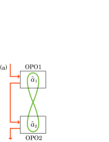
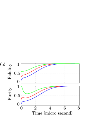
Figure 1: (Color online) (a) Schematic diagram of the cascaded OPOs. (b) Time evolutions of the fidelity $F(t)$ and the purity $P(t)$ of the bipartite cavity state. The parameters are $\kappa=6.0$ MHz and $\epsilon=4.8$ MHz. We take the initial Gaussian states with mean zero and covariance matrices $V(0)=I/2$ (top line), $V(0)=I$ (middle), and $V(0)=2I$ (bottom). Note due to $\langle{\hat{x}(t)}\rangle=0~{}\forall t$, the fidelity is now of the form $F(t)=1/\sqrt{{\rm det}(V(t)+V_{s})}$. The entanglement achieved in this case is $E(V_{s})=1.0986$.

IV Environment engineering for pure Gaussian state preparation

In this section we first address a modification of the condition (ii) of Theorem 1 with different assumption, which is more suited to the concept of environment engineering. In fact, the result allows us to obtain a general procedure for synthesizing a dissipative system whose steady state is uniquely a desired pure Gaussian state. We close this section with some examples.

IV.1 Uniqueness condition for a given Gaussian pure steady state

Theorem 2: Let $V_{s}$ be a covariance matrix corresponding to a pure Gaussian state. Then, this is a unique steady state of the system if and only if

$$\ker\Big{(}V_{s}+\frac{i}{2}\Sigma\Big{)}={\rm range}(K^{\top}),$$ (16)

where $K$ is defined in Eq. (9).

Proof: We begin with the necessary part. In general, for a $n$-mode Gaussian pure state, $V_{s}+i\Sigma/2$ has a $n$-dimensional kernel Simon , while now from the assumption Eq. (11) holds, implying ${\rm range}(K^{\top})\subseteq\ker(V_{s}+i\Sigma/2)$. Hence, showing ${\rm rank}(K^{\top})=n$ completes the proof. Now, as shown in the proof of Theorem 1, from the assumption we have $K\Sigma K^{\top}=0$, implying ${\rm rank}(K^{\top})\leq n$. On the other hand, the uniqueness of the steady state allows us to apply Lemma 1 to get ${\rm rank}(\bar{K}^{\top})=2n$, thus ${\rm rank}(K^{\top})\geq n$. As a result we obtain ${\rm rank}(K^{\top})=n$.

Let us next move to the sufficiency part. First we show that $V_{s}$ satisfying Eq. (16) is a solution of Eqs. (6) and (7), thus that of Eq. (4). Note that now Eq. (6) apparently holds. As seen from the last part of the proof of Theorem 1, Eq. (16) implies $(\Sigma GV_{s}+V_{s}G\Sigma^{\top})K^{\top}=0$, thus we need ${\rm rank}(K^{\prime\top})=2n$ to derive Eq. (7). To show this, assume there exists $\xi\in{\bf R}^{2n}$ such that $K^{\prime}\xi=0$. This leads to $K\xi=0$. Now, from Eq. (16) with $V_{s}$ pure, we have $K\Sigma K^{\top}=0$ and ${\rm rank}(K^{\top})=n$, thus $\ker(K)$ = ${\rm range}(\Sigma K^{\top})$. Then, as $\xi\in{\rm range}(\Sigma K^{\top})$, we can write $\xi=\Sigma K^{\top}\alpha,~{}\exists\alpha\in{\bf C}^{2nm}$. This leads to $0=\Re[(V_{s}+i\Sigma/2)K^{\top}\alpha]=V_{s}\Sigma^{\top}\xi$, thus contradiction to $V_{s}>0$. Consequently, we have ${\rm rank}(K^{\prime\top})=2n$.

Second, to complete the sufficiency part, we show that $V_{s}$ is unique, which is equivalent to that $A$ is Hurwitz. Suppose $A^{\top}\xi=\lambda\xi$ with $\xi\in{\bf C}^{2n}$ and $\lambda\in{\bf C}$. Multiplying Eq. (4) by $\xi^{\dagger}$ from the left and by $\xi$ from the right, we obtain $\Re(\lambda)=-\xi^{\dagger}D\xi/(2\xi^{\dagger}V_{s}\xi)$. Note in general $D\geq 0$ and $V_{s}>0$. But now $\xi^{\dagger}D\xi>0$, because $\xi^{\dagger}D\xi=0$ leads to $K^{\prime}\Sigma^{\top}\xi=0$ and this is contradiction to ${\rm rank}(K^{\prime\top})=2n$. Thus $\Re(\lambda)<0$ and this means that $A$ is Hurwitz. $\blacksquare$

The point of this result is that, while in Theorem 1 the steady state is assumed to be unique, we here assume only that a given state is pure, without assuming its uniqueness. Nonetheless, that state is guaranteed to be a unique steady state if the condition (16) is satisfied. Note again, as seen from the last part of the above proof, that the uniqueness is ensured by ${\rm rank}(K^{\top})=n$, which leads to the Hurwitz property of the matrix $A$. That is, we do not need to check whether $A$ is Hurwitz.

IV.2 Complete parameterization of the dissipative system

Based on the result shown above, we here provide a complete parameterization of the Gaussian dissipative system that uniquely has a pure steady state. This then leads to an explicit procedure for engineering a desired Gaussian dissipative system.

We begin with the fact that any covariance matrix $V_{s}$ corresponding to a pure Gaussian state has the following general representation Menicucci2011 ; Simon88 :

$$V_{s}=\frac{1}{2}SS^{\top},~{}~{}~{}S=\left(\begin{array}[]{cc}Y^{-1/2}&0\\ XY^{-1/2}&Y^{1/2}\\ \end{array}\right),$$ (17)

where $X$ and $Y$ are $n\times n$ real symmetric and real positive definite matrices (i.e., $Y=Y^{\top}>0$), respectively. Note that $S$ is symplectic. With this representation we have

$$V_{s}+\frac{i}{2}\Sigma=\frac{1}{2}\left(\begin{array}[]{c}I\\ Z^{\dagger}\\ \end{array}\right)Y^{-1}(I,~{}Z),$$

where we defined $Z=X+iY$. It was shown in Menicucci2011 that the symmetric matrix $Z$ is useful in graphical calculus for several Gaussian pure states. Because $(I,Z)$ is clearly of rank $n$, we have

$$\ker\Big{(}V_{s}+\frac{i}{2}\Sigma\Big{)}={\rm range}\left(\begin{array}[]{c}-Z\\ I\\ \end{array}\right).$$

Hence, Eq. (16) is equivalent to

$${\rm range}\left(\begin{array}[]{c}-Z\\ I\\ \end{array}\right)={\rm range}(C^{\top},G\Sigma^{\top}C^{\top},\ldots,(G\Sigma^{\top})^{2n-1}C^{\top}).$$

To satisfy this condition, it is necessary that ${\rm range}(C^{\top})$ is included in ${\rm range}(-Z,I)^{\top}$ and that ${\rm range}(-Z,I)^{\top}$ is invariant under $G\Sigma^{\top}$. These conditions are respectively represented by

$$C^{\top}=\left(\begin{array}[]{c}-Z\\ I\\ \end{array}\right)P,~{}~{}~{}G\Sigma^{\top}\left(\begin{array}[]{c}-Z\\ I\\ \end{array}\right)=\left(\begin{array}[]{c}-Z\\ I\\ \end{array}\right)Q,$$ (18)

where $P$ and $Q$ are $n\times m$ and $n\times n$ complex matrices. From the above equations, $K^{\top}$ is represented by

$$K^{\top}=\left(\begin{array}[]{c}-Z\\ I\\ \end{array}\right)(P,~{}QP,\ldots,~{}Q^{2n-1}P).$$

Consequently, the necessary and sufficient condition for ${\rm range}(K^{\top})$ to be identical to ${\rm range}(-Z,I)^{\top}$ is that there exist $P$ and $Q$ satisfying Eq. (18) and the rank condition

$${\rm rank}(P,~{}QP,\ldots,~{}Q^{n-1}P)=n.$$ (19)

Now let us write $G$ in the $2\times 2$ block matrix form $G=(G_{1},G_{2};G_{2}^{\top},G_{3})$, where $G_{1}$ and $G_{3}$ are real $n\times n$ symmetric matrices and $G_{2}$ a real $n\times n$ matrix. Then the latter equation in Eq. (18) leads to

$$G_{1}+G_{2}X+XG_{2}^{\top}+XG_{3}X-YG_{3}Y=0,$$

$$(G_{2}+XG_{3})Y+Y(G_{2}+XG_{3})^{\top}=0.$$

The second equation is equivalent to that there exists a real skew symmetric matrix $\Gamma$ (i.e., $\Gamma+\Gamma^{\top}=0$) satisfying $(G_{2}+XG_{3})Y=\Gamma$. Hence, by writing $R=G_{3}$, we find that $G_{2}$ is expressed as $G_{2}=-XR+\Gamma Y^{-1}$. In this representation, $Q$ is of the form $Q=-iRY-Y^{-1}\Gamma^{\top}$. To conclude, we obtain the complete parameterization of $C$ and $G$ as follows:

$$C=P^{\top}(-Z,~{}~{}I),~{}~{}~{}G=\left(\begin{array}[]{cc}XRX+YRY-\Gamma Y^{-1}X-XY^{-1}\Gamma^{\top}{}{}&-XR+\Gamma Y^{-1}\\ -RX+Y^{-1}\Gamma^{\top}&R\\ \end{array}\right).$$ (20)

Again, $P$ (complex), $R$ (real symmetric), and $\Gamma$ (real skew) are the parameter matrices. We now have a reasonable procedure for environment engineering for pure Gaussian state preparation; that is, the procedure is simply to choose the matrices $P,R$, and $\Gamma$ so that both the dissipative channels $\hat{L}_{k}=c_{k}^{\top}\hat{x}~{}(k=1,\ldots,m)$ and the Hamiltonian $\hat{H}=\hat{x}^{\top}G\hat{x}/2$ with the system matrices given in Eq. (20) have desired structures such as quasi-locality, while, at the same time, $P$ and $Q=-iRY-Y^{-1}\Gamma^{\top}$ satisfy the rank condition (19).

Here we give some remarks.

(i) There always exists the pair of $(P,R,\Gamma)$ satisfying the rank condition Eq. (19), if no restriction is imposed on those matrices; this means that, for any pure Gaussian state, there always exists a Gaussian dissipative system for which that state is the unique steady state.

(ii) The most simple system may be such that $P$ is of rank $n$. In this case we can set $R=\Gamma=0$, implying that the system does not need a nontrivial Hamiltonian but drives the state only by dissipation. This kind of system is called the purely dissipative system. However, we are often in the situation where only $m<n$ dissipative channels can be implemented in reality, due to some reasons related to physical constraints. In this case, the matrix $Q$ needs to be of rank at least $n-m$, meaning that we must add a nontrivial Hamiltonian.

(iii) As stated in Kraus , quasi-locality is indeed essential since otherwise it would be experimentally hard to realize such a dissipative system. It should be noticed that, because $\hat{H}$ is quadratic, it can be always decomposed into the sum of quasi-local Hamiltonians acting on at most two nodes, although those interactions between the nodes do not necessarily have the structure of a target entangled state; in fact, it will be shown in Example 5 that, to generate a chain-type cluster state, a Hamiltonian having a ring-type interaction is added. That is, while in Gaussian case the quasi-locality issue appears only in the part of dissipative channel, this does not mean that the complementary Hamiltonian can readily be implemented.

IV.3 Examples

Example 3: General CV cluster and ${\cal H}$-graph states. Menicucci et al. developed in Menicucci2011 a unified graphical calculus for all pure Gaussian states in terms of the matrix $Z=X+iY$. One of the important results is that the so-called canonical CV cluster state, which can be generated by first squeezing the momentum quadrature of all modes and then applying the controlled $Z$ operations to the modes according to the graph of the cluster, can be generally represented by

$$Z=X+ie^{-2r}I,$$ (21)

where $X$ corresponds to the symmetric adjacency matrix representing the graph structure of the cluster state and $r$ the squeezing parameter. For this state, for instance setting $P=I$ and $Q=0$ in Eq. (18) gives a desired purely dissipative system with channels

$$\left(\begin{array}[]{c}\hat{L}_{1}\\ \vdots\\ \hat{L}_{n}\\ \end{array}\right)=(-X-ie^{-2r}I,I)\hat{x},$$

which have the same structure as that of the target cluster state. Therefore, if each node of the graph is connected to at most three adjacency nodes, each dissipative channel acts on at most three modes too, i.e., it is quasi-local.

Another important state discussed in Menicucci2011 is the ${\cal H}$-graph state; this state is generated by applying the unitary transformation $\hat{U}={\rm exp}(-i\hat{\cal H}t/\hbar)$ with Hamiltonian

$$\hat{\cal H}=i\hbar\kappa\sum_{j,k}W_{jk}(\hat{a}_{j}^{\dagger}\hat{a}_{k}^{\dagger}-\hat{a}_{j}\hat{a}_{k})$$ (22)

to the vacuum states $|{0}\rangle^{\otimes n}$, where $W=(W_{jk})$ is the real symmetric matrix representing the graph. Note that $\hat{\cal H}$ is the sum of the two-mode squeezing Hamiltonians. The corresponding covariance matrix is then given by Eq. (17) with $X=0$ and $Y=e^{-2\alpha W}$, hence

$$Z=ie^{-2\alpha W},$$ (23)

where $\alpha=2\kappa t$. Unlike the CV cluster state representation (21), $Z$ does not necessarily reflect the graph structure of the state. However, for instance when $W$ is self-inverse, i.e., $W^{2}=I$, we have $Z=i\cosh(2\alpha)I-i\sinh(2\alpha)W$. Thus, in this case choosing $P=I$ gives a desired purely dissipative system acting on the nodes in the same manner as the Hamiltonian (22). $\blacksquare$

Example 4: Two-mode squeezed state. In the Gaussian formulation we are often interested in the two-mode squeezed state, as it approximates the so-called EPR state. This is represented as a ${\cal H}$-graph state with the Hamiltonian (22) given by

$$W=\left(\begin{array}[]{cc}0&1\\ 1&0\\ \end{array}\right)~{}~{}\leftrightarrows~{}~{}\hat{\cal H}=2i\hbar\kappa(\hat{a}_{1}^{\dagger}\hat{a}_{2}^{\dagger}-\hat{a}_{1}\hat{a}_{2}).$$

Then the system matrices are $X=0$ and

$$Y=e^{-2\alpha W}=\left(\begin{array}[]{cc}\cosh(2\alpha)&-\sinh(2\alpha)\\ -\sinh(2\alpha)&\cosh(2\alpha)\\ \end{array}\right).$$

The corresponding covariance matrix (17) is given by

$$V_{s}=\frac{1}{2}\left(\begin{array}[]{cc|cc}\cosh(2\alpha)&\sinh(2\alpha)&0&0\\ \sinh(2\alpha)&\cosh(2\alpha)&0&0\\ \hline\cr 0&0&\cosh(2\alpha)&-\sinh(2\alpha)\\ 0&0&-\sinh(2\alpha)&\cosh(2\alpha)\end{array}\right).$$

Let us begin with constructing a purely dissipative system whose unique steady state is the above two-mode squeezed state; in this case, we only need to specify a $2\times 2$ full-rank matrix $P$ to satisfy the rank condition (19). In particular, let us here choose

$$P=\left(\begin{array}[]{cc}i\cosh(\alpha)&i\sinh(\alpha)\\ i\sinh(\alpha)&i\cosh(\alpha)\\ \end{array}\right),$$ (24)

which is clearly of full rank. Then, $C=P^{\top}(-Z,I)=(c_{1},c_{2})^{\top}$ is given by

$$c_{1}=(\mu,~{}\nu,~{}i\mu,~{}-i\nu)^{\top},~{}~{}c_{2}=(\nu,~{}\mu,~{}-i\nu,~{}i\mu)^{\top},$$ (25)

where $\mu=\cosh(\alpha)$ and $\nu=-\sinh(\alpha)$. As a result, the master equation describing this purely dissipative process is given by

$$\frac{d\hat{\rho}}{dt}=\sum_{k=1,2}\Big{(}\hat{L}_{k}\hat{\rho}\hat{L}_{k}^{\dagger}-\frac{1}{2}\hat{L}_{k}^{\dagger}\hat{L}_{k}\hat{\rho}-\frac{1}{2}\hat{\rho}\hat{L}_{k}^{\dagger}\hat{L}_{k}\Big{)},$$ (26)

where $\hat{L}_{1}=\mu\hat{a}_{1}+\nu\hat{a}_{2}^{\dagger}$ and $\hat{L}_{2}=\mu\hat{a}_{2}+\nu\hat{a}_{1}^{\dagger}$. A possible physical realization of this system in a pair of atomic ensembles was discussed in Cirac2 ; Polzik .

Next let us discuss the case where we are allowed to implement only one dissipative channel. As an example we take $P=(i\cosh(\alpha),i\sinh(\alpha))^{\top}$, which corresponds to the first column vector of Eq. (24). This yields $C=c_{1}^{\top}$ in Eq. (25), thus the dissipative channel is $\hat{L}_{1}=\mu\hat{a}_{1}+\nu\hat{a}_{2}^{\dagger}$. We now need to specify a valid $Q$ to satisfy the rank condition (19); in particular let us take a specific Hamiltonian matrix $G$ in Eq. (20) with $R={\rm diag}\{0,~{}1\}$ and $\Gamma=0$, then this leads to

$$Q=-iRY-Y^{-1}\Gamma^{\top}=\left(\begin{array}[]{cc}0&0\\ i\sinh(2\alpha)&-i\cosh(2\alpha)\\ \end{array}\right).$$

It is easily verified that $(P,~{}QP)$ is of full rank, hence the requirement is satisfied. In this case the Hamiltonian $\hat{H}=\hat{x}^{\top}G\hat{x}/2$ is given by

$$\hat{H}=(\hat{q}_{1}\sinh(2\alpha)-\hat{q}_{2}\cosh(2\alpha))^{2}+\hat{p}_{2}^{2}.$$

This Hamiltonian and the dissipative channel $\hat{L}=\mu\hat{a}_{1}+\nu\hat{a}_{2}^{\dagger}$ construct the desired dissipative system. $\blacksquare$

Example 5: 1-dimensional harmonic chain. As a typical cluster state let us take a 1-dimensional (equally weighted) harmonic chain, particularly in the case of four-mode cluster just for simplicity. Within the formalism of the canonical CV cluster state generation, the adjacency matrix $X$ and the graph matrix (21) are respectively given by

$$X=\left(\begin{array}[]{cccc}0&1&&\\ 1&0&1&\\ &1&0&1\\ &&1&0\\ \end{array}\right),~{}~{}Z=\left(\begin{array}[]{cccc}ie^{-2r}&1&&\\ 1&ie^{-2r}&1&\\ &1&ie^{-2r}&1\\ &&1&ie^{-2r}\\ \end{array}\right).$$

A desired purely dissipative system is readily obtained by taking $P=I_{4}$ in Eq. (18), i.e., $C=(-Z,~{}I)$; this means that the four dissipative channels are given by

$$\hat{L}_{1}=(-ie^{-2r}\hat{q}_{1}+\hat{p}_{1})-\hat{q}_{2},$$

$$\hat{L}_{2}=-\hat{q}_{1}+(-ie^{-2r}\hat{q}_{2}+\hat{p}_{2})-\hat{q}_{3},$$

$$\hat{L}_{3}=-\hat{q}_{2}+(-ie^{-2r}\hat{q}_{3}+\hat{p}_{3})-\hat{q}_{4},$$

$$\hat{L}_{4}=-\hat{q}_{3}+(-ie^{-2r}\hat{q}_{4}+\hat{p}_{4}).$$ (27)

Each channel acts on at most three nodes, thus they are quasi-local; Fig. 2 (a) depicts the structure of this environment-system interaction. Note from the above discussion that the general 1-dimensional harmonic chain can also be generated by purely dissipative process with their channels acting on at most three nodes. The finite dimensional counterpart to this result is found in Kraus .

Now we have a natural question; can the chain state be generated by a quasi-local dissipative process acting on at most two adjacency nodes? If this is true, this means that engineering the dissipative environment becomes easier, apart from that we clearly need an additional Hamiltonian. Again let us consider the case of four-mode chain and take $P=(1,0,0,0)^{\top}$, implying that the system has one dissipative channel $\hat{L}_{1}$ in Eq. (IV.3). Note this acts on only two nodes. To determine the Hamiltonian we have some freedom, but let us take in Eq. (20)

$$R=X^{-1}=\left(\begin{array}[]{cccc}0&1&0&-1\\ 1&0&0&0\\ 0&0&0&1\\ -1&0&1&0\\ \end{array}\right),~{}~{}\Gamma=0.$$

This leads to $Q=-iRY-Y^{-1}\Gamma^{\top}=-ie^{-2r}X^{-1}$, and it is readily verified that $(P,QP,Q^{2}P,Q^{3}P)$ is of full rank. Hence, we obtain the positive answer to the question raised above. The matrix $G$ is now of the form

$$G=\left(\begin{array}[]{cc}X+e^{-2r}X^{-1}&-I\\ -I&X^{-1}\\ \end{array}\right).$$

The first $(1,1)$ block matrix indicates that the Hamiltonian $\hat{H}=\hat{x}^{\top}G\hat{x}/2$ has a ring-type structure where the 1-2, 2-3, 3-4, and 4-1 nodes are connected with each other; see the remark (iii) in the previous subsection. Therefore it is concluded that the four-mode harmonic chain state can be generated by the dissipative process where both the dissipative channel and the Hamiltonian quasi-locally act on only two adjacency nodes; the structure of these interactions is shown in Fig. 2 (b). Implementation of this system should be easier than that of the purely dissipative system obtained above, which acts on the nodes through the channels (IV.3). $\blacksquare$

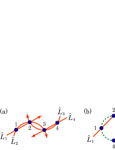
Figure 2: (Color online) (a) Dissipative channels for generating the harmonic chain state. (b) A combination of the dissipative channel (arrow) and the ring-type Hamiltonian (dotted circle) can generate the harmonic chain state.

V Conclusion

In this paper, we have derived the general necessary and sufficient conditions for a Gaussian dissipative system to have a unique pure steady state. In particular, we have provided a complete parameterization of the Gaussian dissipative system satisfying the requirement; this leads to an explicit procedure for engineering a Gaussian dissipative system whose steady state is uniquely a desired pure state.

An important open question is how to construct, in a general framework, a practical dissipative system satisfying a quasi-locality constraint. Although Example 5 demonstrated the feasibility in engineering such a quasi-local dissipative system, that construction method is a heuristic one. Note that in the finite-dimensional case the same problem remains open Kraus .

We can take two approaches to dealing with the problem. The first one is suggested by the recent work by Ticozzi and Viola TicozziViola2011 that, in the finite-dimensional case, characterizes a pure state generated by a dissipative system having a fixed quasi-locality constraint; it was then shown that, based on this result, by switching dissipative channels through output feedback control Wiseman , we are enabled to construct a desired quasi-local dissipative system. It is expected that this idea works in our case as well. Actually, it was shown in Ficek2009 that, with the use of a similar switching method, some Gaussian cluster states can be generated in four-mode atomic ensembles trapped in a ring cavity.

The other approach uses the schematic of quantum state transfer. The basic idea is as follows. First, an $n$-mode target (entangled) Gaussian state of light fields is produced, and then, those fields are independently coupled to $n$ identical bosonic systems in a dissipative way; then, as a result, that state is deterministically transferred to the systems. In this scheme, we need the strong assumption that all the nodes are accessible and independently couple to the fields, but the interactions between the systems and the environment channels are all local. Hence, from the fact that a number of pure Gaussian cluster state of light fields can be produced efficiently with the use of some beam splitters and OPOs Zhang2006 ; vanLoock2007 ; Menicucci2011 , this state-transfer-based approach is expected to be more reasonable. In fact, the dissipation-induced states shown in Cirac1 ; Cirac2 ; Polzik are generated using this technique. Furthermore, one of the authors recently has developed a general theory of this scheme in terms of a quantum stochastic differential equation YamamotoRS2011 .

It would be worth to further examine the above two approaches to make them more useful for engineering a practical dissipative system.

References

- (1) J. F. Poyatos, J. I. Cirac, and P. Zoller, Phys. Rev. Lett. 77, 4728 (1996).
- (2) N. Yamamoto, Phys. Rev. A 72, 024104 (2005).
- (3) A. S. Parkins, E. Solano, and J. I. Cirac, Phys. Rev. Lett. 96, 053602 (2006).
- (4) B. Kraus, H. P. Büchler, S. Diehl, A. Kantian, A. Micheli, and P. Zoller, Phys. Rev. A 78, 042307 (2008).
- (5) S. Diehl, A. Micheli, A. Kantian, B. Kraus, H. P. Büchler, and P. Zoller, Nature Physics 4, 878 (2008).
- (6) F. Ticozzi and L. Viola, IEEE Trans. Automat. Contr. 53, 2048 (2008).
- (7) F. Verstraete, M. M. Wolf, and J. I. Cirac, Nature Physics 5, 633 (2009).
- (8) G. Li, S. Ke, and Z. Ficek, Phys. Rev. A 79, 033827 (2009).
- (9) S. G. Schirmer and X. Wang, Phys. Rev. A 81, 062306 (2010).
- (10) C. A. Muschik, E. S. Polzik, and J. I. Cirac, Phys. Rev. A 83, 052312 (2011).
- (11) H. Krauter, C. A. Muschik, K. Jensen, W. Wasilewski, J. M. Petersen, J. I. Cirac, and E. S. Polzik, Phys. Rev. Lett. 107, 080503 (2011).
- (12) KarlGerdH. Vollbrecht, C. A. Muschik, and J. I. Cirac, Phys. Rev. Lett. 107, 120502 (2011).
- (13) F. Ticozzi and L. Viola, arXiv:1112.4860 (2011).
- (14) S. L. Braunstein and P. van Loock, Rev. Mod. Phys., 77, 513 (2005).
- (15) A. Furusawa and P. van Loock, Quantum Teleportation and Entanglement: A Hybrid Approach to Optical Quantum Information Processing, (Wiley-VCH, Berlin, 2011).
- (16) J. Zhang and S. L. Braunstein, Phys. Rev. A 73, 032318 (2006).
- (17) P. van Loock, C. Weedbrook, and M. Gu, Phys. Rev. A 76, 032321 (2007).
- (18) N. C. Menicucci, S. T. Flammia, and P. van Loock, Phys. Rev. A 83, 042335 (2011).
- (19) N. C. Menicucci, P. van Loock, M. Gu, C. Weedbrook, T. C. Ralph, and M. A. Nielsen, Phys. Rev. Lett. 97, 110501 (2006).
- (20) S. Pirandola, A. Serafini, and S. Lloyd, Phys. Rev. A 79, 052327 (2009).
- (21) H. M. Wiseman and G. J. Milburn, Quantum Measurement and Control (Cambridge University Press, 2009).
- (22) J. Williamson, Am. J. Math. 58, 141 (1936).
- (23) R. Simon, N. Mukunda, and B. Dutta, Phys. Rev. A 49, 1567 (1994).
- (24) R. Simon, E. C. G. Sudarshan, and N. Mukunda, Phys. Rev. A, 37, 3028 (1988).
- (25) M. M. Wolf, G. Giedke, O. Krüger, R. F. Werner, and J. I. Cirac, Phys. Rev. A 69, 052320 (2004).
- (26) H. J. Carmichael, An Open System Approach to Quantum Optics (Springer, Berlin, 1993).
- (27) J. Gough and M. R. James, IEEE Trans. Automat. Contr. 54, 2530 (2009).
- (28) G. Vidal and R. F. Werner, Phys. Rev. A 65, 032314 (2002).
- (29) N. Yamamoto, arXiv:1112.5889 (2011).