Stellar Dynamics and Black Holes

1 Introduction

Chandrasekhar’s most enduring contribution to stellar dynamics is probably dynamical friction. The history of that discovery is fascinating and well known [17]. The first (1942) edition of Principles of Stellar Dynamics contained a chapter entitled “The Time of Relaxation of a Stellar System,” in which Chandrasekhar presented his “completely rigorous” calculation of the rate at which a star is accelerated by encounters with other stars. The result was expressed in terms of $\sum\Delta E^{2}$, the accumulated squared kinetic energy change after some time $\Delta t$. From this, Chandrasekhar defined the relaxation time as

$$\frac{\sum\Delta E^{2}}{E^{2}}=\frac{\Delta t}{T_{E}}$$

and showed that $T_{E}$ was very long, of order $10^{12}$ yr, for a system like the Milky Way. He then defined a second relaxation time , $T_{D}$, in terms of the angular deflection of an orbit and showed that it was equivalent to $T_{E}$.

It was apparently only after publication of his monograph that Chandrasekhar recognized another important consequence of gravitational encounters. In the absence of a decelerating force, repeated encounters would increase the kinetic energy of a star without limit. In a fluid medium, Stokes’ law states that there is a frictional force, proportional to the velocity, that competes with the acceleration. In a paper published in 1943 [3], Chandrasekhar recognized the necessity for such a force in the stellar dynamical case, and showed that the assumption of a Maxwellian velocity distribution implied a simple relation between the frictional force and his previously-derived coefficient of diffusion. He then derived the coefficient of dynamical friction by summing the velocity changes experienced by a test body, in the direction of its motion, as field stars were deflected around it.

Chandrasekhar was clearly proud of the fact that Brownian motion in stellar systems could be treated in such an exact way, compared with the “intuitive character of the assumptions” in the case of fluids [4]. He wrote:

The discussion of the physical foundations of the theory of Brownian motion [in fluids] in the preceding sections has disclosed certain inherent limitations in the theory. The limitations are nowhere more serious than in the circumstance that the coefficients $q$ and $\eta$ [the coefficients of diffusion and friction] are not derived from a microscopic analysis of the individual encounters. It is therefore of interest that stellar dynamics provides a case of Brownian motion in which all phases of the problem can be explcitly analyzed.

In this lecture, I briefly review Chandrasekhar’s derivation of the dynamical friction cofficient, then discuss its application in a few cases that are relevant to the nuclei of galaxies containing massive black holes. I conclude by discussing recent work that extends Chandrasekhar’s ideas to star clusters in which the effects of relativity can not be ignored.

2 Dynamical Friction

In deriving the velocity diffusion coefficients in a stellar system, Chandrasekhar assumed that the instantaneous forces acting on a test star could be separated into two components: a component due to the smoothed-out distribution of matter, and a component arising from chance stellar encounters. He assumed that the encounters were independent, and computed their net effect by integrating the momentum changes of single encounters over the variables defining the relative orbit of the binary (test star, field star) system. The smoothed-out component was assumed to be infinite and homogeneous, implying a constant velocity for the test mass in the absence of encounters. Aside from enforcing istropy in velocity space, no restrictions were placed on $f(\boldsymbol{u})$, the distribution of field star velocities at infinity.

Integrating over all impact parameters $p$, the change per unit interval of time of the test star’s velocity, in a direction parallel to the initial relative motion, is then given by

$$\overline{(\Delta v_{\parallel})}=-{2\pi G^{2}m_{f}\left(m_{f}+m\right)n\over V^{2}}\ln\left(1+p^{2}_{\mathrm{max}}/p_{0}^{2}\right).$$ (1)

Here $m$ and $m_{f}$ are the masses of the test and field star respectively, $n$ is the field star density, $\boldsymbol{V}=\boldsymbol{v}-\boldsymbol{u}$ is the relative velocity of test and field star before the encounter, and

$$p_{0}=\frac{G\left(m_{f}+m\right)}{V^{2}}$$

is the impact parameter corresponding to an angular deflection of $\pi/2$. The final step is the integration over field star velocities. Since equation (1) gives the velocity change in the direction of the initial relative motion, we must multiply it by

$$\frac{\boldsymbol{V}\cdot\boldsymbol{v}}{Vv}=\frac{v-u_{x}}{V}$$

to convert it into a velocity change in the direction of the test star’s motion, assumed here to be along the $x$ axis. The dynamical friction coefficient is then

$$\langle\Delta v_{\parallel}\rangle = \int f(\boldsymbol{u})\,\overline{(\Delta v_{\parallel})}\,{v-{u}_{x}\over V}\boldsymbol{du}$$

$$= -2\pi G^{2}\left(m_{f}+m\right)\rho\int f(\boldsymbol{u}){v-u_{x}\over V^{3}}\ln\left[1+{p_{max}^{2}V^{4}\over G^{2}\left(m_{f}+m\right)^{2}}\right]\boldsymbol{du}$$

where $\rho=m_{f}n$. If the field star distribution is isotropic in velocity space, there are various ways to simplify the integral over velocities. Chandrasekhar chose one that was especially propitious: representing the velocity-space volume element in terms of $u$ and $V$ yields

$$\langle\Delta v_{\parallel}\rangle = -\frac{16\pi^{2}G^{2}\left(m_{f}+m\right)\rho}{v^{2}}\int_{0}^{\infty}f(u)u^{2}{\cal H}\left(v,u,p_{\mathrm{max}}\right)du,$$

$${\cal H}(v,u,p_{max}) = {1\over 8u}\int_{|v-u|}^{v+u}dV\left(1+{v^{2}-u^{2}\over V^{2}}\right)\ln\left[1+{p^{2}_{max}V^{4}\over G^{2}(m_{f}+m)^{2}}\right].$$

This choice separates the integrand into a product of $f$ with a weighting function $\mathcal{H}$ (which Chandrasekhar wrote as $J/8u$).

Chandrasekhar then pointed out an approximation that greatly simplies $\mathcal{H}$. “Under most conditions of practical interest,” he wrote, the argument of the logarithm in equation (LABEL:Equation:df2) “is generally very large compared with unity.” Invoking this assumption, Chandrasekhar derived various approximate forms for $\mathcal{H}$. The last, and simplest, of these was

$${\cal H}=\left\{\begin{array}[]{ll}\ln\Lambda&\mbox{if $v>u$,}\\ 0&\mbox{if $v<u$}\end{array}\right.$$

which corresponds to treating the logarithmic term in equation (LABEL:Equation:df2) as a constant. In this approximation, the dynamical friction coefficient becomes

$$\langle\Delta v_{\parallel}\rangle=-\frac{16\pi^{2}G^{2}\left(m_{f}+m\right)\rho\ln\Lambda}{v^{2}}\int_{0}^{v}f(u)u^{2}du.$$ (3)

Equation (3) contains the beautiful result that the dynamical friction force is proportional to the number of field stars moving more slowly (at infinity) than the test star.

For the “Coulomb logarithm”, Chandrasekhar suggested the form

$$\ln\Lambda=\ln\left[\frac{p_{\mathrm{max}}\overline{u^{2}}}{G(m_{f}+m)}\right].$$

As for the parameter $p_{\mathrm{max}}$, Chandrasekhar and von Neumann [6] argued that the effect of gravitational interactions should be cut off at roughly the interparticle distance. Later authors [e.g. 7] have generally advocated larger values for $p_{\mathrm{max}}$: the physical size of the system, or the density scale length.

Following the derivation of equation (3), Chandrasekhar wrote: “As we shall see presently, it is precisely on this account [i.e. on account of the fact that only stars with $u<v$ contribute to the force] that dynamical friction appears in our present analysis.”

Maybe I missed it, but I could not find where in his paper Chandrasekhar justifies this statement. In any case, it is fun to play devil’s advocate, and ask how dynamical friction acts in cases where this is not true.

A student of Chandrasekhar’s, Marvin Lee White, considered one such case [20]. If $p_{\mathrm{max}}$ is equated with the half-mass radius of a stellar cluster, then using the Virial Theorem, it is easy to show that $\ln\Lambda\approx\ln(N)$ with $N$ the number of stars in the cluster. For sufficiently small $N$, the assumption of large $\ln\Lambda$ breaks down. White showed that in a cluster containing just a few hundred stars, a significant fraction of the frictional force acting on a test mass could come from stars with $u>v$.

Two other cases come to mind, both in the context of massive black holes (MBHs).

• A MBH near the center of a galaxy experiences a kind of random walk due to perturbations from stars. Assuming equipartition of kinetic energy, its velocity will be small, $v\approx(m_{\star}/M)^{1/2}\sqrt{\overline{u^{2}}}$. But if $v$ is small, the logarithmic term in equation (LABEL:Equation:df2) will be close to zero for all field stars with $u<v$. Either the frictional force acting on the MBH is much less than implied by equation (3), or most of the force must come from field stars with $u>v$.

• There are physically reasonable models for the distribution of stars around a MBH that imply few or no stars with velocities less than some value; for instance, the local circular velocity. In such cases, Chandrasekhar’s approximate formula would predict no frictional force on a body moving in a circular orbit; all the force would have to come from the fast-moving stars.

Consider first the Brownian motion example. Chandrasekhar (1943) showed that the rms velocity of the test star is given by

$$v^{2}_{\mathrm{rms}}=\frac{3}{2}\left|\frac{\langle(\Delta v_{\parallel})^{2}\rangle}{\langle\Delta v_{\parallel}\rangle/v}\right|.$$

Expanding the diffusion coefficients about $v=0$,

$$\langle\Delta v_{\parallel}\rangle = -Av+Bv^{3}\ldots,$$

$$\langle(\Delta v_{\parallel})^{2}\rangle = C+Dv^{2}\ldots$$

so that $v^{2}_{\mathrm{rms}}=3C/2A$. The coefficients $A$ and $C$ are obtained from the low-velocity limit of equation (LABEL:Equation:df2), and the equivalent expression for $\langle(\Delta v_{\parallel})^{2}\rangle$ [2]. The results are

$$A = {32\over 3}\pi^{2}G^{2}M\rho\int_{0}^{\infty}f(u){p_{max}^{2}u^{4}/G^{2}M^{2}\over 1+p_{max}^{2}u^{4}/G^{2}M^{2}}{du\over u},$$ (4a)

$$C = {16\over 3}\pi^{2}G^{2}m_{\star}\rho\int_{0}^{\infty}f(u)\log\left(1+{p_{max}^{2}u^{4}\over G^{2}M^{2}}\right)u\,du$$ (4b)

where $M$ is the MBH mass. It is evident from the first of these expressions that field stars of every velocity contribute to the dynamical friction force. If the field star velocity distribution is a Maxwellian, the result of the integrations is

$$A=4\sqrt{6\pi}G^{2}M\rho\left(\overline{u^{2}}\right)^{-3/2}\ln\Lambda^{\prime},\ \ \ \ \ C=\frac{8}{3}\sqrt{6\pi}G^{2}m_{\star}\rho\left(\overline{u^{2}}\right)^{-1}\ln\Lambda^{\prime}$$

where

$$\ln\Lambda^{\prime}\equiv{1\over 2}\int_{0}^{\infty}dz\ e^{-z}\ln\left(1+\frac{4p_{\mathrm{max}}^{2}(\overline{u^{2}})^{2}}{9G^{2}M^{2}}z^{2}\right)\approx\ln\sqrt{1+{2p^{2}_{max}(\overline{u^{2}})^{2}\over 9G^{2}M^{2}}}.$$

The rms velocity of the MBH has the expected value, $(m_{\star}\overline{u^{2}}/M)^{1/2}$, regardless of the value of $\ln\Lambda^{\prime}$ . But returning to the question of which stars generate the frictional force: the integrand of equation (4a) peaks at $u\approx(GM/p_{\mathrm{max}})^{1/2}$. Furthermore, $p_{\mathrm{max}}$ in the case of a MBH near the center of a galaxy is expected to be comparable to the MBH influence radius $GM/\overline{u^{2}}$ [13, 15]. It follows that most of the frictional force responsible for Brownian motion of a MBH comes from field stars with speeds similar to their rms value, and not exclusively, or even predominantly, from the slow-moving stars (Figure 1).

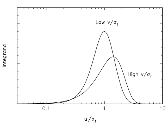
Figure 1: Relative contribution of different field-star velocities to the dynamical friction integral, equation (4a), in the limit of low and high velocities of the test mass, assuming a Maxwellian distribution of field-star velocities with one-dimensional velocity dispersion $\sigma_{f}=(\overline{u^{2}}/3)^{1/2}$. $p_{\mathrm{max}}=GM/\sigma_{f}^{2}$ has been assumed, appropriate for a massive test body moving at the center of a galaxy. Roughly the same set of field stars dominates the frictional force, whether the test mass is moving very slowly or very fast.

The second case mentioned above was a test mass orbiting around a MBH at the center of a galaxy. Suppose that the stars, which are responsible for the frictional force, are distributed around the MBH with density $\rho(r)\propto r^{-\gamma}$. Assuming an isotropic velocity distribution, their phase space density is given by

$$f\propto(-E_{f})^{\gamma-3/2}\propto\left(2v_{c}^{2}-u^{2}\right)^{\gamma-3/2}$$ (5)

where $v_{c}=(GM/r)^{1/2}$ is the local circular speed. For $\gamma<3/2$, $f$ diverges at $u=2^{1/2}v_{c}$, and in the limit $\gamma=1/2$, $f$ is a delta-function at $u=2^{1/2}v_{c}$. In other words, in a $\rho\propto r^{-1/2}$ density cusp around a MBH, none of the stars at $r$ is moving more slowly than the local circular speed. The dynamical friction formula in its approximate form (3) would predict zero frictional force in this case.

It so happens that the distribution of stars at the centers of galaxies containing MBHs is often as flat as $\rho\sim r^{-1/2}$ [8]; indeed this appears to be the case at the center of the Milky Way [1]. One explanation is that these low-density cores were “carved out” by binary MBHs [10]. But whatever their origin, the argument just given suggests that dynamical friction in such cores must be due almost entirely to stars that move faster than the inspiralling body. Of course, the frictional force on a test mass at a distance $r$ from the MBH would come partly from stars at greater $r$, and some of these stars will have smaller $u$. Chandrasekhar’s theory does not make clear predictions in the case of inhomogeneous systems. It would be interesting to address this question using an $N$-body code.

Why do the two populations – stars with $u<v$ and stars with $u>v$ – contribute in such different ways to the frictional force? One way to visualize this is to compute the dynamical-friction “wake,” the overdensity of stars behind the test body that is responsible for the decelerating force. If the field star distribution is infinite and homogeneous, and if the test body’s velocity is rectilinear and unaccelerated (all assumptions that were made by Chandrasekhar), the wake is time-independent in a frame following the test mass, and its density can be computed using Jeans’s theorem given the distribution of field star velocities at infinity [16].

Figure 2 shows the result of such a calculation, assuming that the velocity distribution at infinity is given by equation (5) with $\gamma=5/4$ and that the test body’s velocity is $v_{c}$. For this choice of $f$, the “fast” stars dominate both the total density at infinity, as well as the density in the wake.

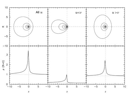
Figure 2: Dynamical friction wake around a massive object moving through an infinite homogeneous stellar system. The panels at the top show contours of the density, in a frame that follows the massive body (located at the origin); motion is to the right at constant speed $v$. The left panel shows the total density, the middle panel shows the density contributed only by stars with velocity at infinity less than that of the massive body, and the right panel shows the contribution from the complement of stars that move faster than $v$. The lower panels show the density along a line through the moving body in the direction of its motion. In the usual approximation, first derived by Chandrasekhar, one computes the dynamical friction force ignoring the fast-moving stars. This figure helps to explain why that is a good approximation, even if the fast stars dominate the total density.

However the shapes of the two, partial density wakes are very different. The wake created by the fast stars is elongated counter to the direction of the test body’s motion, reducing the net force that it exerts on the test mass. In addition, the change in density between the upstream and downstream sides of the test mass is less for the fast stars than for the slow stars. These two differences are responsible for the small contribution of the fast stars to the total frictional force, in spite of their higher density at infinity and in the wake.

3 Relativistic Dynamical Friction

In 1969, Edward E. Lee, a PhD student of Chandrasekhar’s, re-derived the expression for the dynamical friction force, using the first post-Newtonian (1PN) approximation for the relative orbit of test and field stars [12]. Lee motivated his calculation in the following way: “These effects of general relativity, in the lowest order, may be relevant for consideration of stellar encounters in dense systems such as are now contemplated in a number of contexts.” Lee’s final expression for the relativistic dynamical friction coefficient was fairly complex, and he did not go so far as to evaluate it in the case of a particular velocity distribution. But given $f(u)$, Lee noted that the relativistic formula predicted a higher frictional force than the non-relativistic formula, due to the greater relative deflection in the 1PN approximation, and also because the relativistic transformation from the inertial frame to the frame of the test mass introduces an additional term into the force.

4 Relativistic Stellar Dynamics

Massive black holes were not yet quite in vogue at the time that Lee wrote his thesis. It is now commonly assumed that all massive galaxies have them. Given Chandrasekhar’s fundamental contributions to the theory of gravitational encounters, and to the theory of black holes [5], gravitational encounters between stars orbiting near a MBH is a topic that he might naturally have been interested in.

A black hole is a compact object, and from the point of view of a star that orbits far outside the event horizon, its gravitational field should be nearly indistinguishable from that of a Newtonian point mass. But the Newtonian approximation breaks down for matter that passes within a few gravitational radii:

$$r_{g}\equiv\frac{GM}{c^{2}}\approx 5\times 10^{-8}\mathrm{pc}\left(\frac{M}{10^{6}M_{\odot}}\right)$$

since the orbital velocity at such distances approaches the speed of light.

At first sight, one is struck by the enormous difference between $r_{g}$ and $r_{\mathrm{infl}}$, the radius of gravitational of influence of a MBH:

$$r_{\mathrm{infl}}\equiv\frac{GM}{\sigma_{\star}^{2}}\approx 1\mathrm{pc}\left(\frac{M}{10^{6}M_{\odot}}\right)\left(\frac{\sigma_{\star}}{100\mathrm{km\ s}^{-1}}\right)^{-2}$$

where $\sigma_{\star}$ is the stellar velocity dispersion at $r\gtrsim r_{\mathrm{infl}}$. These two equations suggest that the vast majority of stars within the influence sphere are too far from the MBH for relativity to be important.

This conclusion turns out to be misleading, for a couple of reasons. First: the effects of relativity depend less on the size of an orbit than on its distance of closest approach to the MBH. The lowest-order corrections to the Newtonian equations of motion have amplitudes that are of order ${\cal P}^{-1}$ where ${\cal P}$ is the penetration parameter:

$${\cal P}\equiv(1-e^{2})\frac{a}{r_{g}}=\left(1+e\right)\frac{r_{p}}{r_{g}}.$$

Here, $a$ and $e$ are the semi-major axis and eccentricity of the orbit, and $r_{p}=(1-e)a$ is the radius of periapsis. It turns out that the feeding of stars and compact objects to MBHs occurs predominantly from very eccentric orbits. For instance, capture of stellar-mass BHs by MBHs – so-called “extreme-mass-ratio inspiral” (EMRI) – is believed to take place from orbits with semi-major axes $a\lesssim 0.1$ pc and eccentricities in the range $0.999-0.99999$ [11]. For such orbits, ${\cal P}$ can be of order unity even though the orbit extends outward to thousands or tens of thousands of gravitational radii.

A second reason why the effects of relativity can not be ignored has to do with the way in which stars get placed onto orbits of such high eccentricity. The dominant mechanism is believed to be torques, i.e. non-radial forces, that arise from the slightly aspherical distribution of matter near a MBH [18]. These torques remain effective as long as orbits near the MBH – both the orbit of the star being torqued, and the orbits of the torquing stars – maintain their orientations; any mechanism that causes orbits to precess (for instance) tends to randomize the torques. Relativistic precession of the periapsis – or, as it is know in the Solar system, precession of the perihelion – is such a mechanism. If the time scale for relativistic precession is shorter than the time time required for the torques to do their work, feeding of objects to the MBH will be greatly inhibited. This relativistic quenching effect turns out to be of major importance in the EMRI problem.

Consider a star on a bound orbit near a MBH, with semi-major axis $a$ and angular momentum $\boldsymbol{L}$. The orbit-averaged torque $|\boldsymbol{F}\times\boldsymbol{r}|$ that another star of mass $m$ exerts on it is $\sim Gm/a$. The residual torque due to $N$ stars, randomly oriented about the MBH at about the same radius, is $\left|\boldsymbol{T}\right|\approx\sqrt{N}Gm/a$. Over some span of time, this orbit-averaged torque is nearly constant, and the angular momentum of a test star’s orbit responds by changing linearly with time, $\Delta L/\Delta t\approx T\approx\sqrt{N}Gm/a$. This coherent evolution continues for a time $\sim t_{\mathrm{coh}}$, where $t_{\mathrm{coh}}$ is the time scale associated with the most rapid mechanism that randomizes the torques, i.e. the orientations of the orbits resposible for the torques.

Sufficiently far from a MBH, coherence breaking is due mostly to the same distributed mass that generates the torques. Modelling that mass as spherical, the associated precession time is

$$t_{M}\approx P\frac{M}{M_{\star}}$$ (6)

where $P$ is the orbital period, $M$ is the MBH mass, and $M_{\star}$ is the distributed mass within $r=a$. (There is also a dependence on $e$, in the sense that eccentric orbits precess more slowly.) This time is believed to be of order $10^{4}$ yr in the case of the so-called S stars, bright young stars at the center of the Milky Way whose orbits can be tracked astrometrically; the S stars have $0.01\ \mathrm{pc}\lesssim a\lesssim 0.1\ \mathrm{pc}$ and $10^{1}\mathrm{yr}\lesssim P\lesssim 10^{3}\mathrm{yr}$ [9].

Closer to the MBH, relativistic effects become important. The most important precessional time scales associated with relativistic corrections to the equations of motion are

$$t_{S} = \frac{1}{6}{\cal P}P$$

$$t_{J} = \frac{1}{4}{\cal P}^{3/2}\chi^{-1}P$$

$$t_{Q} = \frac{1}{3}{\cal P}^{2}\chi^{-2}P$$

The first of these refers to precession of the periapse; the subscript $S$ indicates that this effect is due to the Schwarzschild (zero spin) part of the metric. This “Schwarzschild precession” is similar to, but in the opposite sense of, precession due to the distributed mass. The other two time scales are associated with the spin ($J$) and quadrupole moment ($Q$) of the MBH. $t_{J}$ is the time for precession of the line of nodes due to frame-dragging, and $t_{Q}$ is the nodal precession time resulting from the nonsphericity of space-time around a spinning hole. (The quadrupole precession rate also depends on the inclination of the orbit with respect to the MBH spin axis.) These latter two times are functions of $\chi$, the dimensionless spin of the MBH: writing the hole’s spin angular momentum as $\boldsymbol{J}$,

$$\boldsymbol{\chi}\equiv\boldsymbol{J}\frac{GM^{2}}{c^{2}}$$

and $\chi=1$ for a maximally-spinning hole.

The time scales for relativistic precession defined above decrease as $(1-e)$, or faster, as $e\rightarrow 1$. If torques from the $\sqrt{N}$ asymmetries in the stellar distribution drive the eccentricity of a test star’s orbit to a sufficiently large value, relativistic effects will dominate its precession. At some critical precession rate (i.e. eccentricity), the sign of the torque as experienced by the orbit will fluctuate with such a high frequency that its net effect over one precessional period will be negligible: in other words, relativity will “quench” the effects of the torques.

This critical eccentricity can be estimated as follows. As shown above, the residual torque produced by $N$ stars is

$$T\approx\frac{Gm}{a}\sqrt{N(a)}\approx\frac{1}{\sqrt{N(a)}}\frac{GM_{\star}(a)}{a}$$

where $N(a)=M_{\star}(a)/m$ is the number of stars, of mass $m$, within radius $r=a$. Writing $L=\left[GMa(1-e^{2})\right]^{1/2}$ for the test star’s angular momentum, the time scale over which $L$ is changed by this torque is

$$\left|\frac{1}{L}\frac{dL}{dt}\right|^{-1}\approx\sqrt{N(a)}\frac{M}{M_{\star}(a)}\left[\frac{a^{3}(1-e^{2})}{GM}\right]^{1/2}.$$

The condition that this time be shorter than the relativistic precession time $t_{S}$ is

$$\ell>\ell_{\mathrm{SB}}\approx\frac{r_{g}}{a}\frac{M}{M_{\star}(a)}\sqrt{N(a)}$$

where

$$\ell\equiv L/L_{c}=(1-e^{2})^{1/2}$$

is the ratio of the test star’s angular momentum to its circular value. In terms of eccentricity,

$$\left(1-e^{2}\right)_{\mathrm{SB}} \approx 2\left(\frac{r_{g}}{a}\right)^{2}\left(\frac{M}{m}\right)^{2}\frac{1}{N}$$

$$\approx 2\times 10^{-5}\left(\frac{a}{0.01\mathrm{pc}}\right)^{-2}\left(\frac{M}{10^{6}M_{\odot}}\right)^{4}\left(\frac{m}{10M_{\odot}}\right)^{-2}\left(\frac{N}{10^{2}}\right)^{-1}.$$

This “Schwarzschild barrier” (so called since it arises from the Schwarzschild part of the metric) sets an effective upper limit to the eccentricty of the test star.

What happens when a star (or stellar remnant) “strikes” the barrier? Figure 3 shows one example, extracted from an $N$-body simulation [14]. The orbit’s eccentricity first oscillates, about a lower bound given by equation (4). The oscillations have a period equal to $t_{S}$; they reflect the periodically changing effects of the torques on the precessing star. After some elapsed time – roughly 6 precessional periods in this case – the star is “reflected” from the barrier by the torques, back to smaller values of the eccentricity.

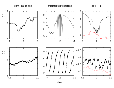
Figure 3: An eccentric orbit near a massive black hole, extracted from an $N$-body integration [14]. Plotted are the semi-major axis, argument of periapse and eccentricity versus time, at low (top) and high (bottom) time resolutions. In the plots of eccentricity vs. time, the lower (red) curves show the predicted location of the Schwarzschild barrier. Changes in the predicted barrier location reflect changes in the semi-major axis, via eq. (4).

The elapsed time until reflection is just the coherence time $t_{\mathrm{coh}}$ defined above. The orbits of all the other stars are also precessing: not as rapidly as the test star (which has the highest eccentricity), but at a lower rate – in the example shown in Figure 3, the distributed mass determines the precession rate of most stars, via equation (6). After a time of $t_{\mathrm{coh}}\approx t_{\mathrm{M}}$, the net torque due to the other stars has changed its direction and the angular momentum of the test star responds by decreasing, taking the star away from the barrier.

The $N$-body experiments from which Figure 3 was derived were designed to generate EMRIs, i.e. inspiral of stellar remnants into the MBH. For this to happen, the remnants must sometimes penetrate the Schwarzschild barrier.

Penetration does occur, but because the coherent torquing – or “resonant relaxation” – is quenched by the effects of relativity, all that is left is the kind of random gravitational scattering treated by Chandrasekhar, or “non-resonant relaxation”. It turns out that the rate at which objects get scattered past the angular momentum barrier is accurately predicted by Chandrasekhar’s formulae. The only additional consideration arises from the fact that stars remain near the barrier only for a limited time, $\Delta t\approx t_{\mathrm{coh}}$, before the changing background torques pull them away; to be effective, the encounters described by Chandrasekhar’s formulae must decrease the test body’s angular momentum, by an amount greater than the amplitude of the oscillations shown in Figure 3, in a time less than $t_{\mathrm{coh}}$. This argument correctly reproduces the EMRI capture rate observed in the simulations, and also turns out to imply a minimum semi-major axis, of order $10^{-3}$ pc, below which stars can not be driven past the barrier, either by resonant or non-resonant relaxation [14].

The collisional dynamics of relativistic stellar systems is a fascinatingly rich topic. It is a shame that Chandrasekhar is not here to sort it out for us.

- [1] Buchholz, R. M., Schödel, R., & Eckart, A., Astronomy and Astrophysics, 499, 483 (2009)
- [2] Chandrasekhar, S., Principles of Stellar Dynamics (University of Chicago Press, Chicago, 1942)
- [3] Chandrasekhar, S., The Astrophysical Journal, 97, 255 (1943)
- [4] Chandrasekhar, S., Reviews of Modern Physics, 21, 383 (1949)
- [5] Chandrsekhar, S., The Mathematical Theory of Black Holes (New York: Clarendon Press), (1983)
- [6] Chandrasekhar, S., & von Neumann, J., The Astrophysical Journal, 95, 489 (1942)
- [7] Cohen, R. S., Spitzer, L., & Routly, P. M., Physical Review, 80, 230 (1950)
- [8] Côté, P., et al., The Astrophysical Journal, 671, 1456 (2007)
- [9] Gillessen, S., Eisenhauer, F., Trippe, S., Alexander, T., Genzel, R., Martins, F., & Ott, T., The Astrophysical Journal, 692, 1075 (2009)
- [10] Graham, A. W., The Astrophysical Journal Letters, 613, L33 (2004)
- [11] Hopman, C., & Alexander, T., The Astrophysical Journal, 645, 1152 (2006)
- [12] Lee, E. P., The Astrophysical Journal, 155, 687 (1969)
- [13] Maoz, M., Monthly Notices of the Royal Astronomical Society, 263, 75 (1993)
- [14] Merritt, D., Alexander, T., Mikkola, S., & Will, C., The Physical Review D, in press
- [15] Milosavljević, M., & Merritt, D., The Astrophysical Journal, 563, 34 (2001)
- [16] Mulder, W. A., Astronomy and Astrophysics, 117, 9 (1983)
- [17] Padmanabhan, T., Current Science, 70, 784 (1996)
- [18] Rauch, K. P., & Tremaine, S., New Astronomy, 1, 149 (1996)
- [19] Schutz, B. F., Journal of Astrophysics and Astronomy, 17, 183 (1996)
- [20] White, M. L., The Astrophysical Journal, 109, 159 (1949)