Motion of position-dependent mass as a damping-antidamping process: Application to the Fermi gas and to the Morse potential

Abstract

The object of this paper is to investigate, classically and quantum mechanically, the relation existing between the position-dependent effective mass and damping-antidamping dynamics. The quantization of the equations of motion is carried out using the geometric interpretation of the motion, and we compare it with the one based on the ordering ambiguity scheme. Furthermore, we apply the obtained results to a Fermi gas of damped-antidamped particles, and we solve the Schrödinger equation for an exponentially increasing (decreasing) mass in the presence of the Morse potential.

I Introduction

In the course of the development of the quantum theory, Schrödinger’s equation has played a central role land . It represents the basic tool for studying the behavior of many quantum systems ranging from nuclei greiner to solid-state compounds kittel . Very often, one deals with systems whose masses are constant in time and in space. Fortunately, this leads in many cases to exact results regarding the energy spectra and the eigenfunctions of the associated Hamiltonians, as is the case for, among others, the harmonic oscillator and the hydrogen atom.

There exist, on the other hand, physical systems for which the mass exhibits the property of being time and/or position dependent. In particular, the motion of position-dependent effective mass (PDEM) has been the subject of a great deal of investigations, owing to its connection with the description of various physical systems such as quantum dots dots ; dots2 , semiconductors semi ; semi1 ; semi2 ; semi3 ; semi4 ; semi5 ; semi6 ; semi7 , metal clusters metal , ${\rm{}^{3}He}$ clusters he , and quantum liquids liquid . Depending on the intended application, many techniques have been used in order to study the PDEM motion chro ; chro1 ; chro2 ; chro3 ; chro4 ; chro5 ; chro6 ; chro7 ; chro8 ; chro9 ; chro10 ; chro11 ; chro12 ; chro13 ; chro14 ; chro15 ; the standard approach consists in solving the Schrödinger equation, where one inevitably has to deal with the nontrivial ordering problem of the momentum operator and the mass in the kinetic energy part of the PDEM Hamiltonian ord .

In this paper, we explore the PDEM motion from a dynamical point of view, and we investigate its damping-antidamping character both classically and quantum mechanically. Generally speaking, the damping of classical particles is described by a frictional force that is proportional to the velocity (i.e., a force which is an odd function of the velocity) odd . In effect, the system under investigation is dissipative and is, quite often, non-Hamiltonian, making it difficult to quantize the equations of motion. This is the reason for which different approaches are adopted in the attempt to achieve a satisfactory quantum mechanical description of damped systems weiss ; gardiner . Moreover, frictional forces that depend on the square of the velocity are known from hydrodynamics. As we shall see latter, the PDEM motion is tightly related to such forces, which may display antidamping behavior due to the fact that they are even functions of the velocity. The question that naturally arises is whether the corresponding equations of motion can be quantized using the standard technique. We shall be concerned with the answer of this question in the first part of this paper.

The Fermi gas has found many applications in various fields of physics, like nuclear physics hofman , and solid-state physics kittel . Hence it is of interest to investigate the consequences of the spatial dependence of the mass on the properties of this system. In this spirit, we feel tempted to extend the analysis to the molecular domain, by studying the PDEM motion under the effect of the Morse potential morse .

The paper is organized as follows. In Section II we establish the relation between the PDEM and damping-antidamping motion. There, the quantization of the equations of motion is carried out through the geometric interpretation of the dynamics, which enables us to find the stationary states corresponding to quasi-free particles for particular forms of the spatial dependence of the mass. Section III is devoted to the application of the obtained results to a gas of damped-antidamped particles at zero and nonzero temperatures; the emphasis will be on the consequences on the pressure and the specific heat of the gas. In Section IV, we solve the Schrödinger equation when the particle is endowed with exponentially decreasing (or increasing) mass, under the effect of the Morse potential, to determine the energy spectra and the eigenfunctions. The paper is ended with a summary.

II Damping-antidamping interpretation of the PDEM motion

II.1 Classical treatment

In one dimension, the Hamiltonian corresponding to a position-dependent effective mass $m(q)=m_{0}M(q)$, where $M(q)$ is a dimensionless positive function of the generalized coordinate $q$, is given by

$$H(p,q)=\frac{p^{2}}{2m(q)}+V(q)=\frac{p^{2}}{2m_{0}M(q)}+V(q).$$ (1)

Here $V(q)$ is the potential, and $p$ denotes the generalized canonical momentum conjugate to $q$, that is:

$$\{q,p\}=1,\qquad\{q,q\}=\{p,p\}=0,$$ (2)

where the curly braces denote Poisson Brackets. Using the canonical equations of motion

$$\dot{q} = \frac{\partial H}{\partial p},$$

$$\dot{p} = -\frac{\partial H}{\partial q},$$ (3)

it can easily be shown that

$$\dot{p}=\frac{1}{2}[\nabla_{q}m(q)]{\dot{q}}^{2}-\nabla_{q}V(q),$$ (4)

where $\nabla_{q}\equiv\partial_{q}$, and the dot designates the derivation with respect to time. Taking into account the fact that $\dot{m}(q)=\dot{q}\nabla_{q}m(q)$, it immediately follows that

$$\ddot{q}=-\frac{1}{2m(q)}[\nabla_{q}m(q)]{\dot{q}}^{2}-\frac{1}{m(q)}\nabla_{q}V(q).$$ (5)

Now multiplying both sides of the latter equation by the constant $m_{0}$ yields

$$m_{0}\ddot{q}=-\Bigl{[}\frac{m_{0}}{2M(q)}\nabla_{q}M(q)\Bigr{]}{\dot{q}}^{2}-\nabla_{q}\Biggl{\{}\int\limits_{q}\frac{1}{M(q)}\nabla_{q}V(q)dq+V_{0}\Biggr{\}},$$ (6)

where $V_{0}$ is a constant. Clearly, (6) is the equation of motion corresponding to a particle of constant mass, $m_{0}$, moving in one dimension, subjected to the effect of two forces; the first one being proportional to the square of the velocity:

$$F_{d}=-\Bigl{[}\frac{m_{0}}{2M(q)}\nabla_{q}M(q)\Bigr{]}{\dot{q}}^{2},$$ (7)

while the second one is a conservative force, derived from the effective potential

$$V_{\rm eff}(q)=\int\limits_{q}\frac{1}{M(q)}\nabla_{q}V(q)dq+V_{0}.$$ (8)

Integrating by parts, we can rewrite $V_{\rm eff}$ as

$$V_{\rm eff}(q)=\frac{V(q)}{M(q)}+\int\limits_{q}\frac{V(q)}{M(q)^{2}}\nabla_{q}M(q)dq+V_{0}.$$ (9)

Let us now take a look at equation (7). It is clear that $F_{d}$ is an even function of the generalized velocity $\dot{q}$, meaning that the nature of the force is dictated by the explicit forms of $M(q)$ and $V(q)$. Suppose that the latter is such that the particle is constrained to move in some definite region of space. Consequently, $F_{d}$ is of frictional nature (the particle is decelerated) when $\dot{q}>0$ and $\nabla_{q}M(q)>0$ or $\dot{q}<0$ and $\nabla_{q}M(q)<0$. On the contrary the particle gains acceleration (antidamping) if $\dot{q}>0$ and $\nabla_{q}M(q)<0$ or $\dot{q}<0$ and $\nabla_{q}M(q)>0$. This may be better seen by noting that $\nabla_{q}M(q)=\dot{M}(q)/\dot{q}$. When $V(q)$ is zero and $M(q)$ monotonic, the particle (which we call quasi-free) is either damped or antidamped depending on its initial velocity. We thus come to the conclusion that the PDEM motion is equivalent to the damping-antidamping dynamics of a particle with constant mass subjected to a force proportional to the square of the velocity.

In what follows we shall prove the converse. To this end, consider the following equation of motion

$$m_{0}\ddot{q}=-\phi(q)\dot{q}^{2}-\nabla_{q}U(q;\alpha),$$ (10)

where $U(q;\alpha)$ is a potential depending on some parameter $\alpha$. Our task here is to find the Hamiltonian from which equation (10) is derived. First of all notice that a first integral for (10), which we denote by $I$, is a function of $q$ and $\dot{q}$, satisfying

$$\frac{dI(q,\dot{q})}{dt}=\dot{q}\frac{\partial I}{\partial q}+\ddot{q}\frac{\partial I}{\partial\dot{q}}=0.$$ (11)

This means that

$$\dot{q}\frac{\partial I}{\partial q}-\frac{1}{m_{0}}\Bigl{[}\phi(q)\dot{q}^{2}+\nabla_{q}U(q;\alpha)\Bigr{]}\frac{\partial I}{\partial\dot{q}}=0.$$ (12)

Let $\mathcal{C}$ denote the family of curves in the $(q,\dot{q})$ plane, for which $dI/dq=0$ holds. Hence along these curves we have that

$$\frac{\partial I}{\partial q}+\frac{d\dot{q}}{dq}\frac{\partial I}{\partial\dot{q}}=0.$$ (13)

Comparing (12) and (13), we get the following first-order ordinary differential equation

$$\frac{d\dot{q}}{dq}=-\frac{1}{m_{0}}\phi(q)\dot{q}-\frac{1}{m_{0}\dot{q}}\nabla_{q}U(q;\alpha).$$ (14)

We seek a solution in the form

$$\dot{q}=f(q){\rm e}^{-\frac{1}{m_{0}}\int_{q}\phi(q)dq}$$ (15)

where $f(q)$ is some function of $q$. By inserting the proposed solution into (14), we get after some algebra

$$\frac{df^{2}}{dq}=-\frac{2}{m_{0}}{\rm e}^{\frac{2}{m_{0}}\int_{q}\phi(q)dq}\nabla_{q}U(q;\alpha).$$ (16)

This can easily be integrated, and we get

$$f(q)^{2}=-\frac{2}{m_{0}}\int\limits_{q}{\rm e}^{\frac{2}{m_{0}}\int_{q}\phi(q)dq}\nabla_{q}U(q;\alpha)dq+C.$$ (17)

Here $C$ is a constant of integration characteristic of the curves $\mathcal{C}$. Finally, the general solution of (14) is

$$\dot{q}^{2}=C{\rm e}^{-\frac{2}{m_{0}}\int_{q}\phi(q)dq}-\frac{2}{m_{0}}{\rm e}^{-\frac{2}{m_{0}}\int_{q}\phi(q)dq}\int\limits_{q}{\rm e}^{\frac{2}{m_{0}}\int_{q}\phi(q)dq}\nabla_{q}U(q;\alpha)dq.$$ (18)

We solve for $C$ to obtain

$$C(q,\dot{q})=\dot{q}^{2}{\rm e}^{\frac{2}{m_{0}}\int_{q}\phi(q)dq}+\frac{2}{m_{0}}\int\limits_{q}{\rm e}^{\frac{2}{m_{0}}\int_{q}\phi(q)dq}\nabla_{q}U(q;\alpha)dq.$$ (19)

The simplest choice we can make for the first integral of the equation of motion is

$$I(q,\dot{q})=\frac{1}{2}m_{0}g(\alpha)C(q,\dot{q})+K(\alpha),$$ (20)

where $g(\alpha)$ is a dimensionless positive function of the parameter $\alpha$ and where $K(\alpha)$ has the dimension of energy.

According to int1 ; int2 ; int3 ; int4 , the Lagrangian of the system is given in terms of the first integral by

$$L=\dot{q}\int\frac{I(q,\dot{q})}{\dot{q}^{2}}d\dot{q}.$$ (21)

A straightforward calculation yields

$$L=\frac{1}{2}m_{0}g(\alpha)\dot{q}^{2}{\rm e}^{\frac{2}{m_{0}}\int_{q}\phi(q)dq}-g(\alpha)\int\limits_{q}{\rm e}^{\frac{2}{m_{0}}\int_{q}\phi(q)dq}\nabla_{q}U(q;\alpha)dq-K(\alpha).$$ (22)

It is now easy to show that the generalized momentum is equal to

$$p=\frac{\partial L}{\partial\dot{q}}=m_{0}g(\alpha){\rm e}^{\frac{2}{m_{0}}\int_{q}\phi(q)dq}\dot{q}.$$ (23)

Consequently, the Hamiltonian corresponding to (10) is given by

$$H(q,p) = \dot{q}p-L$$ (24)

$$= \frac{p^{2}}{2m_{0}g(\alpha)}{\rm e}^{-\frac{2}{m_{0}}\int_{q}\phi(q)dq}+g(\alpha)\int\limits_{q}{\rm e}^{\frac{2}{m_{0}}\int_{q}\phi(q)dq}\nabla_{q}U(q;\alpha)dq+K(\alpha).$$

Clearly, this is the Hamiltonian for a position-dependent mass

$$m(q)=m_{0}g(\alpha){\rm e}^{\frac{2}{m_{0}}\int_{q}\phi(q)dq}$$ (25)

subjected to the effective potential

$$U_{\rm eff}(q;\alpha)=g(\alpha)\int\limits_{q}{\rm e}^{\frac{2}{m_{0}}\int_{q}\phi(q)dq}\nabla_{q}U(q;\alpha)dq+K(\alpha).$$ (26)

As an example consider the motion of the particle under the effect of the force $-\eta\dot{q}^{2}$ ($\phi(q)=\eta>0$), in the presence of the Morse potential morse

$$U(q;\alpha)=A({\rm e}^{-2\alpha q}-2{\rm e}^{-\alpha q})$$ (27)

with $A,\alpha>0$. From equation (26), it follows that when $\alpha\neq\eta/m_{0}$ and $\alpha\neq 2\eta/m_{0}$,

$$U_{\rm eff}(q;\alpha)=g(\alpha)A\Biggl{[}\frac{\exp\{2(\tfrac{\eta}{m_{0}}-\alpha)q\}}{1-\tfrac{\eta}{m_{0}\alpha}}-\frac{2\exp\{(\tfrac{2\eta}{m_{0}}-\alpha)q\}}{1-\tfrac{2\eta}{m_{0}\alpha}}\Biggl{]}+K(\alpha).$$ (28)

On the other hand if $\alpha=\eta/m_{0}$, then

$$U_{\rm eff}(q;\alpha)=2g(\alpha)A\Bigl{[}\exp(2\alpha q)-\alpha q\Bigr{]}+K(\alpha),$$ (29)

whereas for $\alpha=2\eta/m_{0}$ we find that

$$U_{\rm eff}(q;\alpha)=2g(\alpha)A\Bigl{[}\exp(-2\alpha q)+\alpha q\Bigr{]}+K(\alpha).$$ (30)

Obviously, $g(\alpha)$ and $K(\alpha)$ are not the same for all the cited circumstances; note, however, that while $K(\alpha)$ may arbitrarily be chosen (additive constant), $g(\alpha)$ should be reduced to unity when $\eta\to 0$. Even though, the choice one can make for $g(\alpha)$ still seems to be not unique. It should be stressed that, generally speaking, different Hamiltonians describing the same classical system may yield completely different quantum behaviors.

To illustrate the importance of the inclusion of the function $g$ we calculate the minimum of the effective potential $U_{\rm eff}$ appearing in equation (28):

$$U_{\rm eff}^{\rm min}=Ag(\alpha)\Biggl{[}\frac{1}{1-\tfrac{\eta}{m_{0}\alpha}}-\frac{2}{1-\tfrac{2\eta}{m_{0}\alpha}}\Biggl{]}+K(\alpha).$$ (31)

We observe that the quantity $Q=\frac{1}{1-\tfrac{\eta}{m_{0}\alpha}}-\frac{2}{1-2\tfrac{\eta}{m_{0}\alpha}}$ blows up in the neighborhoods of $\alpha=\eta/m_{0}$ and $\alpha=2\eta/m_{0}$. Indeed, $Q\to-\infty$ when $\eta/(m_{0}\alpha)\to 1^{+}$ or $2\eta/(m_{0}\alpha)\to 1^{-}$, whereas $Q\to+\infty$ when $\eta/(m_{0}\alpha)\to 1^{-}$ or $2\eta/(m_{0}\alpha)\to 1^{+}$, which, obviously, is physically unacceptable. The only way to remove these singularities consists in choosing the following form for the function $g(\alpha)$:

$$g(\alpha)=\widetilde{g}(\alpha)\Bigl{|}(1-\tfrac{\eta}{m_{0}\alpha})(1-\tfrac{2\eta}{m_{0}\alpha})\Bigr{|}$$ (32)

where $\widetilde{g}(\alpha)$ is a regular positive dimensionless function of $\alpha$. Therefore the effective potential reads

$$U_{\rm eff}(q;\alpha) = \widetilde{g}(\alpha)A\Biggl{[}{\rm{sgn}}\Bigl{(}1-\tfrac{\eta}{m_{0}\alpha}\Bigr{)}\Bigl{|}1-\tfrac{2\eta}{m_{0}\alpha}\Bigr{|}\exp\Bigl{\{}2(\tfrac{\eta}{m_{0}}-\alpha)q\Bigr{\}}$$ (33)

$$- 2\ {\rm{sgn}}\Bigr{(}1-\tfrac{2\eta}{m_{0}\alpha}\Bigr{)}\Bigl{|}1-\tfrac{\eta}{m_{0}\alpha}\Bigr{|}\exp\Bigl{\{}(\tfrac{2\eta}{m_{0}}-\alpha)q\Bigr{\}}\Bigr{]}+K(\alpha).$$

As a result, the mass becomes $\alpha$ dependent.

II.2 Quantization

From a geometric point of view, the Hamiltonian (1) describes, strictly speaking, the motion of a particle with constant mass $m_{0}$ in a one-dimensional space whose metric is defined by

$$ds^{2}=M(q)dq^{2}.$$ (34)

The corresponding Hamiltonian operator reads

$$\hat{H}=-\frac{\hbar^{2}}{2m_{0}}\Delta+V(q),$$ (35)

where $\Delta$ denotes the Laplacian operator. From the differential geometry we know that the Laplacian operator in the curvilinear coordinates $x_{\mu}$ with metric tensor $g_{\mu\nu}$ is given by

$$\Delta=\frac{1}{\sqrt{{\rm det(g_{\mu\nu})}}}\sum\limits_{\mu,\nu}\frac{\partial}{\partial x_{\mu}}\sqrt{{\rm det(g_{\mu\nu})}}g_{\mu\nu}^{-1}\frac{\partial}{\partial x_{\nu}}.$$ (36)

It follows that the time-dependent Schrödinger equation, in our case, takes the form

$$\Biggl{[}-\frac{\hbar^{2}}{2m_{0}\sqrt{M(q)}}\frac{\partial}{\partial q}\frac{1}{\sqrt{M(q)}}\frac{\partial}{\partial q}+V(q)\Biggr{]}\psi(q,t)=i\hbar\frac{\partial\psi(q,t)}{\partial t}.$$ (37)

In turn the wave function $\psi(q,t)$ should be normalized according to

$$\int_{-\infty}^{\infty}|\psi(q,t)|^{2}\sqrt{M(q)}dq=1,{}$$ (38)

which actually arises from the fact that the line element is equal to $\sqrt{M(q)}dq$. On the other hand we can write:

$$i\hbar\Bigl{(}\psi^{*}\frac{\partial\psi}{\partial t}+\psi\frac{\partial\psi^{*}}{\partial t}\Bigr{)} = -\frac{\hbar^{2}}{2\sqrt{m(q)}}\Biggl{[}\frac{\psi^{*}}{\sqrt{m(q)}}\Delta_{q}\psi+\frac{\nabla_{q}\psi\nabla_{q}\psi^{*}}{m(q)^{1/2}}-\frac{\nabla_{q}\psi\nabla_{q}\psi^{*}}{m(q)^{1/2}}$$ (39)

$$- \frac{1}{2}\frac{\nabla_{q}m(q)}{m(q)^{3/2}}\psi^{*}\nabla_{q}\psi-\frac{\psi}{\sqrt{m(q)}}\Delta_{q}\psi^{*}+\frac{1}{2}\frac{\nabla_{q}m(q)}{m(q)^{3/2}}\psi\nabla_{q}\psi^{*}\Biggr{]}$$

$$= -\frac{\hbar^{2}}{2\sqrt{m(q)}}\nabla_{q}\Biggl{(}\frac{\psi^{*}}{\sqrt{m(q)}}\nabla_{q}\psi-\frac{\psi}{\sqrt{m(q)}}\nabla_{q}\psi^{*}\Biggr{)},$$

where $\nabla_{q}\equiv\partial_{q}$, and $\Delta_{q}\equiv\partial^{2}_{q}$. Now by noting that the gradient in the $q$ direction is ${\rm grad}_{q}\equiv\widetilde{\nabla}_{q}\equiv M(q)^{-1/2}\nabla_{q}$, the equation of local conservation of probability takes the form

$$\frac{\partial|\psi|^{2}}{\partial t}+\widetilde{\nabla}_{q}j=0,$$ (40)

with the probability current

$$j=\frac{\hbar}{2im_{0}}[\psi^{*}(q,t)\widetilde{\nabla}_{q}\psi(q,t)-\psi(q,t)\widetilde{\nabla}_{q}\psi^{*}(q,t)].$$ (41)

Moreover, if we assume that $m(q)$ does not depend explicitly on time, then we get another continuity equation in the usual Cartesian space:

$$\frac{\partial\tilde{\rho}}{\partial t}+\nabla_{q}\tilde{j}=0,$$ (42)

where

$$\tilde{\rho}(q,t)=|\psi(q,t)|^{2}\sqrt{M(q)}=|\psi(q,t)M(q)^{1/4}|^{2},$$ (43)

and where

$$\tilde{j}(q,t) = \frac{\hbar}{2im_{0}\sqrt{M(q)}}\Biggl{[}\psi^{*}\nabla_{q}\psi-\psi\nabla_{q}\psi^{*}\Biggr{]}$$ (44)

$$= \frac{\hbar}{2im_{0}}\Biggl{[}\frac{\psi^{*}}{M(q)^{1/4}}\nabla_{q}\Biggl{(}\frac{\psi}{M(q)^{1/4}}\Biggr{)}-\frac{\psi}{M(q)^{1/4}}\nabla_{q}\Biggl{(}\frac{\psi^{*}}{M(q)^{1/4}}\Biggr{)}\Biggr{]}.$$

Hence it is constructive to define a new wave function

$$\varphi=\frac{\psi}{M(q)^{1/4}}.$$ (45)

After some algebra, it can be shown that the latter wave function satisfies the Schrödinger equation

$$-\frac{\hbar^{2}}{2m_{0}M(q)}\frac{\partial^{2}\varphi}{\partial q^{2}}+{\widetilde{V}}(q)\varphi=i\hbar\frac{\partial\varphi}{\partial t},$$ (46)

where the effective potential is

$$\widetilde{V}(q)=V(q)+\frac{\hbar^{2}}{8m_{0}M(q)}\Biggl{[}\frac{5(\nabla_{q}M(q))^{2}}{4M(q)^{2}}-\frac{\Delta_{q}M(q)}{M(q)}\Biggr{]}.$$ (47)

Case of a quasi-free particle in one dimension

Suppose that the potential $V(q)$ is identically equal to zero in the whole space, and that the position dependence of the mass of the particle is given by

$$m(q)=m_{0}\ {\rm e}^{-\frac{2\eta}{m_{0}}q}.$$ (48)

We shall look for the stationary states satisfying the time-independent Schrödinger equation

$$\hat{H}\psi(q)=E\psi(q),$$ (49)

where $E>0$ is the energy of the particle. Taking into account (37) we get

$$\frac{d^{2}\psi}{dq^{2}}+\frac{\eta}{m_{0}}\frac{d\psi}{dq}+\frac{2m_{0}E}{\hbar^{2}}{\rm e}^{-(2\eta/m_{0})q}\psi=0,$$ (50)

By the change of variable $\xi={\rm e}^{-(\eta/m_{0})q}$, the above equation reduces to the simple second-order differential equation

$$\frac{d^{2}\psi}{d\xi^{2}}+\frac{2m_{0}^{3}E}{\hbar^{2}\eta^{2}}\psi=0,$$ (51)

which can easily be solved. Hence the general solution of (50) is

$$\psi(q) = C_{1}(\eta)\exp\Biggl{\{}i\sqrt{\frac{2m_{0}^{3}E}{\hbar^{2}\eta^{2}}}{\rm e}^{-(\eta/m_{0})q}\Biggr{\}}+C_{2}(\eta)\exp\Biggl{\{}-i\sqrt{\frac{2m_{0}^{3}E}{\hbar^{2}\eta^{2}}}{\rm e}^{-(\eta/m_{0})q}\Biggr{\}}$$ (52)

$$= C_{1}(\eta)\psi^{-}(q)+C_{2}(\eta)\psi^{+}(q).$$

The meaning of the notations $\psi^{\pm}(q)$ is clear from the above equation. We redefine the constants $C_{1}$ and $C_{2}$ in such a way that $\psi$ takes the form (assume $\eta>0$)

$$\psi(q) = C_{1}(\eta)\exp\Biggl{\{}-i\sqrt{\frac{2m_{0}^{3}E}{\hbar^{2}\eta^{2}}}(1-{\rm e}^{-\frac{\eta}{m}q})\Biggr{\}}+C_{2}(\eta)\exp\Biggl{\{}i\sqrt{\frac{2m_{0}^{3}E}{\hbar^{2}\eta^{2}}}(1-{\rm e}^{-\frac{\eta}{m}q})\Biggr{\}}.$$ (53)

Now the limit of constant mass ($\eta\to 0$) may be obtained by a Taylor expansion of the exponential function; this yields

$$\lim\limits_{\eta\to 0}\psi(q)=\widetilde{C}_{1}\ {\rm e}^{-ikq}+\widetilde{C}_{2}\ {\rm e}^{ikq},$$ (54)

where $k=\sqrt{2m_{0}E/\hbar^{2}}$ and where $\widetilde{C}_{1,2}=\lim_{\eta\to 0}C_{1,2}(\eta)$. It is clear that the above equation represents the usual expression of the wave function for a free particle.

Consequently, we can interpret $\psi^{+}(q)$ as the wave function of the particle when it is moving to the right, whereas $\psi^{-}(q)$ describes the motion in the opposite direction. Indeed, it can easily be verified that the probability current density corresponding to $\psi^{\pm}$ is equal to $\pm\sqrt{2m_{0}E}/(\hbar)$. Since $\nabla_{q}m(q)<0$, we conclude that $\psi^{-}$ corresponds to the damping of the particle; on the contrary, $\psi^{+}$ describes the antidamping behavior of our quantum system.

Now let us examine the transmission and the reflection of the particle from the rectangular potential wall $U(q)=U_{0}\theta(q-a)$ where $U_{0}>0$ and $\theta(q)$ is the heaviside function. We further assume, for the sake of generality, that the mass of the particle is given by

$$m(q)=m_{0}\exp\{-2(\eta_{1}\theta(a-q)+\eta_{2}\theta(q-a))q/m_{0}\}.$$ (55)

Note that the solution of the Schrödinger equation when the potential is $U(q)=U_{0}={\rm const}$ can be obtained by simply replacing $E$ in (52) by $E-U_{0}$.

First we need to determine the conditions that should be satisfied by the wave function and its derivative at the discontinuity point $a$. To this end let us multiply both sides of equation (49) by $\sqrt{M(q)}$ and integrate between $a-\epsilon$ and $a+\epsilon$, where $\epsilon$ is a small number; we find

$$-\frac{\hbar^{2}}{2m_{0}}\lim\limits_{\epsilon\to 0}\Biggl{[}\frac{1}{\sqrt{M(q)}}\frac{d\psi}{dq}\biggl{|}_{a+\epsilon}-\frac{1}{\sqrt{M(q)}}\frac{d\psi}{dq}\biggl{|}_{a-\epsilon}\Biggr{]}=\lim\limits_{\epsilon\to 0}\int_{a-\epsilon}^{a+\epsilon}\bigl{[}E-U(q)\bigr{]}\sqrt{M(q)}dq.$$ (56)

The right-hand side of the latter equation is identically equal to zero since the quantity under the integral sign is bounded (we assume that $M(q)$ is bounded in the interval $[a-\epsilon,a+\epsilon])$. Hence

$$\Biggl{(}\frac{1}{\sqrt{M(q)}}\frac{d\psi}{dq}\Biggr{)}\biggl{|}_{a^{-}}=\Biggl{(}\frac{1}{\sqrt{M(q)}}\frac{d\psi}{dq}\Biggr{)}\biggl{|}_{a^{+}},$$ (57)

which simply expresses the fact that the gradient of the wave function should be continuous at the discontinuity point. The continuity of the wave function itself follows from

$$0=\lim\limits_{\epsilon\to 0}\int_{a-\epsilon}^{a+\epsilon}\frac{1}{\sqrt{M(q)}}\frac{d\psi}{dq}\sqrt{M(q)}dq=\psi(q)|_{a^{+}}-\psi(q)|_{a^{-}}.$$ (58)

Taking into account the above boundary conditions, together with the fact that the probability current corresponding to $\psi^{\pm}$ is independent of the position $q$, we can show that the reflection coefficient has exactly the same form as in the constant mass case, namely:

$$R=\Biggl{[}\frac{1-\sqrt{1-\tfrac{U_{0}}{E}}}{1+\sqrt{1-\tfrac{U_{0}}{E}}}\Biggr{]}^{2},$$ (59)

independent of $\eta$.

The Schrödinger equation we have used thus far was derived from the geometric interpretation of the PDEM motion. Nevertheless, it is worthwhile to point out that in dealing with the PDEM problems, one often writes the kinetic energy part of the Hamiltonian in the form

$$\hat{T}=\frac{1}{4m_{0}}[M(q)^{\nu}\hat{p}M(q)^{\mu}\hat{p}M(q)^{\kappa}+M(q)^{\kappa}\hat{p}M(q)^{\mu}\hat{p}M(q)^{\nu}].$$ (60)

Here $\mu$, $\nu$, and $\kappa$ are von Roos’ ambiguity parameters, which satisfy the condition $\mu+\nu+\kappa=-1$ ord . Let us consider, for instance, the following Hamiltonian ($V=0$)

$$\hat{H}=\frac{1}{2m_{0}}\hat{p}\frac{1}{M(q)}\hat{p},$$ (61)

obtained from (60) by setting $\nu=\kappa=0$. It can easily be verified that the Schrödinger equation with this Hamiltonian yields

$$\frac{d^{2}\psi}{dq^{2}}+\frac{2\eta}{m_{0}}\frac{d\psi}{dq}+\frac{2m_{0}E}{\hbar^{2}}{\rm e}^{-(2\eta/m_{0})q}\psi=0,$$ (62)

which differs from equation (50) by the factor $2$. Now by making the change of variable $\xi=\sqrt{2m_{0}^{3}E/\hbar^{2}\eta^{2}}{\rm e}^{-\eta q/m_{0}}$, we end up with

$$\xi^{2}\psi^{{}^{\prime\prime}}-\xi\psi^{{}^{\prime}}+\xi^{2}\psi=0.$$ (63)

To eliminate the minus sign in front of the first derivative we further assume that $\psi=\xi\phi$. We then find that the function $\phi$ satisfies

$$\xi^{2}\phi^{{}^{\prime\prime}}+\xi\phi^{{}^{\prime}}+(\xi^{2}-1)\phi=0.$$ (64)

This is the well-known differential equation for the Bessel functions of order 1 abr ; thus the solution of (63) is:

$$\phi(\xi)=C_{1}(\eta)J_{1}(\xi)+C_{2}(\eta)Y_{1}(\xi),$$ (65)

where $J_{1}$ and $Y_{1}$ denote, respectively, the Bessel functions of the first and second kinds. It follows that the general solution of equation (62) is given by

$$\psi(q)=\sqrt{\frac{2m_{0}^{3}E}{\hbar^{2}\eta^{2}}}{\rm e}^{-\eta q/m_{0}}\Biggl{[}C_{1}J_{1}\Bigl{(}\sqrt{{2m_{0}^{3}E}/{\hbar^{2}\eta^{2}}}{\rm e}^{-\eta q/m_{0}}\Bigr{)}+C_{2}Y_{1}\Bigl{(}\sqrt{{2m_{0}^{3}E}/{\hbar^{2}\eta^{2}}}{\rm e}^{-\eta q/m_{0}}\Bigr{)}\Biggr{]}.$$ (66)

Besides the fact that this wave function describes a completely different quantum behavior as compared to the one obtained above in (52), here the smooth transition to the constant mass case cannot be made. Notice that this transition was possible in (52) because of the multiplicative property of the exponential function, which does not hold for the Bessel functions. In particular, the explicit form of the probability current density corresponding to (66) turns out to be quite involved.

III Fermi gas of damped-antidamped particles and effective mass tensor

In this section we generalize the concept of the Fermi gas to the case where the particles, which we suppose identical with mass $m$ (we omit for now the subscript 0), are individually subjected to the effect of three forces; each of these is proportional to the square of the component of the mechanical velocity along the corresponding coordinates axis of the three-dimensional configuration space, that is,

$$F_{q}=\eta v_{q}^{2},\qquad q\equiv x,y,z.$$ (67)

Using the results of the previous section, we find that such a system admits the Hamiltonian

$$H=\sum\limits_{i=1}^{N}\Biggl{(}\frac{p_{x_{i}}^{2}}{2m}{\rm e}^{2\eta x_{i}/m}+\frac{p_{y_{i}}^{2}}{2m}{\rm e}^{2\eta y_{i}/m}+\frac{p_{z_{i}}^{2}}{2m}{\rm e}^{2\eta z_{i}/m}\Biggl{)},$$ (68)

where $N$ is the number of particles. Accordingly, we may regard the gas as a system of particles in a medium where each particle is characterized by the diagonal effective mass tensor ${\rm diag}(m{\rm e}^{-2\eta x/m},m{\rm e}^{-2\eta y/m},m{\rm e}^{-2\eta z/m})$.

We assume that the gas is in thermal equilibrium at temperature $k_{B}T=1/\beta$ ($k_{B}$ denotes Boltzmann’s constant) and is completely contained in the cube $-L\leq x,y,z\leq L$. This is the only acceptable form of the intervals, otherwise the symmetry with respect to the change of the sign of the force will be violated. Under the latter assumptions the classical partition function reads

$$\mathcal{Z} = \frac{1}{N!h^{3N}}\prod\limits_{k=1}^{3N}\int\limits_{-L}^{L}dq\int\limits_{-\infty}^{\infty}dp\exp\Bigl{\{}-\frac{\beta p^{2}}{2m}\ {\rm e}^{2\eta q/m}\Bigr{\}}$$ (69)

$$= \frac{1}{N!h^{3N}}\Bigl{(}\frac{2\pi m}{\beta}\Bigr{)}^{3N/2}\prod\limits_{k=1}^{N}\overbrace{\Biggl{(}\int\limits_{-L}^{L}dq\ {\rm e}^{-\eta q/m}\Biggr{)}^{3}}\limits^{V(\eta)}.$$

Clearly, $V(\eta)$ represents the volume in the 3D curvilinear space with the metric tensor ${\rm diag}({\rm e}^{-\eta x/m},{\rm e}^{-\eta y/m},{\rm e}^{-\eta z/m})$, which justifies once more the use of the geometric interpretation of the motion. The integral in (69) can easily be carried out, yielding (for $\eta>0$)

$$\mathcal{Z}=\frac{1}{N!h^{3N}}\Bigl{(}\frac{2\pi m}{\beta}\Bigr{)}^{3N/2}\Biggl{[}\frac{2m}{\eta}\sinh\Bigl{(}\eta L/m\Bigr{)}\Biggr{]}^{3N}.$$ (70)

Hence, by Stirling’s formula, the free energy of the system can be written as

$$F = -k_{B}T\ln\mathcal{Z}$$ (71)

$$= -k_{B}TN\Biggl{\{}\frac{3}{2}\ln T+\ln\Biggl{[}\frac{1}{N}(2m/\eta)^{3}\sinh^{3}\Bigl{(}\eta L/m\Bigr{)}\Biggr{]}+\ln\frac{(2\pi mk_{B})^{3/2}e}{h^{3}}\Biggr{\}}.$$

Knowing the explicit form of the free energy, one can calculate the diverse thermodynamical quantities characterizing the gas. In particular, the pressure turns out to be equal to

$$P=-\Bigl{(}\frac{\partial F}{\partial V}\Bigr{)}_{TN}=\frac{Nk_{B}T}{V(\eta)},$$ (72)

with

$$V(\eta)=\Biggl{[}\frac{2m}{\eta}\sinh\Bigl{(}\eta L/m\Bigr{)}\Biggr{]}^{3}.$$ (73)

Thus

$$PV(\eta)=Nk_{B}T,$$ (74)

implying that at constant temperature, the pressure decreases as $\eta$ increases (see discussion bellow). The chemical potential, on the other hand, reads

$$\mu=\Bigl{(}\frac{\partial F}{\partial N}\Bigr{)}_{TV}=3k_{B}T\ln\Biggl{[}\frac{h\eta N^{1/3}}{2\sqrt{2\pi k_{B}m^{3}T}\sinh\Bigl{(}\eta L/m\Bigr{)}}\Biggr{]}.$$ (75)

In a similar way we find that the internal energy of the gas is

$$U=-T^{2}\Bigl{(}\frac{\partial F/T}{\partial T}\Bigr{)}_{VN}=\frac{3}{2}Nk_{B}T,$$ (76)

which does not depend on $\eta$. As a direct consequence, we conclude that the specific heat is equal to $C_{V}=\frac{3}{2}Nk_{B}$. Hence, although the pressure is inversely proportional to $\eta$, the classical analysis reveals no dependence of the internal energy and the specific heat on the applied force, in contrast to what one might expect. As we shall see bellow the quantum mechanical treatment of the problem does resolve this issue.

To achieve this aim, we first look for the discrete energy levels of the gas, assuming that the potential is zero within the region of space containing the particles and is infinite outside it. The wave function of every particle of the gas is simply given by the product of the wave functions associated with the one-dimensional motion in each coordinates axis, that is

$$\Psi(x,y,z)=\psi(x)\psi(y)\psi(z),$$ (77)

where

$$\psi(q)=C_{1}(\eta)\exp\Biggl{\{}i\sqrt{\frac{2m^{3}E}{\hbar^{2}\eta^{2}}}{\rm e}^{-(\eta/m)q}\Biggr{\}}+C_{2}(\eta)\exp\Biggl{\{}-i\sqrt{\frac{2m^{3}E}{\hbar^{2}\eta^{2}}}{\rm e}^{-(\eta/m)q}\Biggr{\}}.$$ (78)

Since this should vanish at the edges of the interval $-L\leq q\leq L$, it follows that

$$\exp\Biggl{\{}2i\sqrt{\frac{2m^{3}E}{\hbar^{2}\eta^{2}}}{\rm e}^{(\eta/m)L}\Biggr{\}}=\exp\Biggl{\{}2i\sqrt{\frac{2m^{3}E}{\hbar^{2}\eta^{2}}}{\rm e}^{-(\eta/m)L}\Biggr{\}},$$ (79)

which yields the quantized energy levels ($q\equiv x,y,z$)

$$E_{n_{q}}=\Biggl{(}\frac{\hbar^{2}\eta^{2}}{8m^{3}}\Biggr{)}\frac{\pi^{2}n_{q}^{2}}{\sinh^{2}\Bigl{(}\eta L/m\Bigr{)}},\qquad n_{q}=1,2,3,\cdots$$ (80)

Hence the eigenenergies corresponding to (77) read

$$E_{n_{x}n_{y}n_{z}}=\frac{\hbar^{2}\eta^{2}\pi^{2}}{8m^{3}\sinh^{2}\Bigl{(}\eta L/m\Bigr{)}}(n_{x}^{2}+n_{y}^{2}+n_{z}^{2}).$$ (81)

The wave function (78), in turn, takes the form (we drop the subscript $q$)

$$\psi_{n}(q)=C^{(n)}(\eta)\Biggl{\{}\exp\Biggl{(}-i\sqrt{\frac{2m^{3}E_{n}}{\hbar^{2}\eta^{2}}}{\rm e}^{-(\eta/m)q}\Biggr{)}-\exp\Biggl{(}i\sqrt{\frac{2m^{3}E_{n}}{\hbar^{2}\eta^{2}}}({\rm e}^{-\eta q/m}-2{\rm e}^{-\eta L/m})\Biggr{)}\Biggr{\}}.$$ (82)

The constant $C^{(n)}(\eta)$ can be determined from the normalization condition

$$\int\limits_{-L}^{L}|\psi_{n}(q)|^{2}{\rm e}^{-\eta q/m}dq=1.$$ (83)

After some algebra, one obtains

$$|C^{(n)}(\eta)| = \sqrt{\frac{\eta}{2m}}\Biggl{\{}2\sinh\Bigl{(}\eta L/m\Bigr{)}-\frac{1}{2k(E_{n})}\sin\Bigl{(}2k(E_{n}){\rm e}^{-\eta L/m}\Bigr{)}$$ (84)

$$\times \Bigl{[}\cos\Bigl{(}2k(E_{n}){\rm e}^{-\eta L/m}\Bigr{)}-\cos\Bigl{(}2k(E_{n}){\rm e}^{\eta L/m}\Bigr{)}\Bigr{]}+\frac{1}{2k(E_{n})}\cos\Bigl{(}2k(E_{n}){\rm e}^{-\eta L/m}\Bigr{)}$$

$$\times \Bigl{[}\sin\Bigl{(}2k(E_{n}){\rm e}^{-\eta L/m}\Bigr{)}-\sin\Bigl{(}2k(E_{n}){\rm e}^{\eta L/m}\Bigr{)}\Bigr{]}\Biggr{\}}^{-1/2}$$

$$= \sqrt{\frac{\eta}{2m}}\Biggl{\{}2\sinh\Bigl{(}\eta L/m\Bigr{)}-\frac{1}{2k(E_{n})}\sin\Bigl{[}4k(E_{n})\sinh\Bigl{(}\eta L/m\Bigr{)}\Bigr{]}\Biggr{\}}^{-1/2},$$

with $k(E_{n})=\sqrt{2m^{3}E_{n}/\hbar^{2}\eta^{2}}$.

For completeness we also display the quantity

$$\mathcal{P}_{n}(L) = \int\limits_{-L}^{L}|\psi_{n}(q)|^{2}dq$$ (85)

$$= \frac{2m}{\eta}|C^{(n)}(\eta)|^{2}\Biggl{\{}2L+\sin\Bigl{(}2k(E_{n}){\rm e}^{-\eta L/m}\Bigr{)}$$

$$\times \Bigl{[}{\rm Si}\Bigl{(}2k(E_{n}){\rm e}^{-\eta L/m}\Bigr{)}-{\rm Si}\Bigl{(}2k(E_{n}){\rm e}^{\eta L/m})\Bigr{)}\Bigr{]}+\cos\Bigl{(}2k(E_{n}){\rm e}^{-\eta L/m}\Bigr{)}$$

$$\times \Bigl{[}{\rm Ci}\Bigl{(}2k(E_{n}){\rm e}^{-\eta L/m}\Bigr{)}-{\rm Ci}\Bigl{(}2k(E_{n}){\rm e}^{\eta L/m}\Bigr{)}\Bigr{]}\Biggr{\}},$$

where

$${\rm Si}(x) = \int\limits_{0}^{x}\frac{\sin(\xi)}{\xi}\ d\xi,$$ (86)

$${\rm Ci}(x) = \int\limits_{0}^{x}\frac{\cos(\xi)}{\xi}\ d\xi$$ (87)

are, respectively, the sine and the cosine integral functions abr . In figure 1 we display the quantity $\rho_{n}(q)=|\psi_{n}|^{2}\sqrt{M(q)}$ as a function of $q$ for some values of $\eta$, $L$ and $n$. We see that the probability of finding the particle is maximum in the region of space where the mass is large (see the discussion bellow). The same observation holds for $|\psi_{n}|^{2},$ as indicated in figure 2.

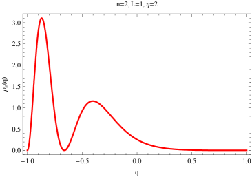
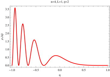
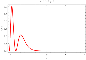
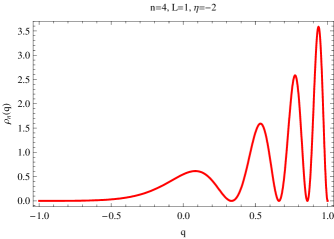
Figure 1: (Color online) The probability density $\rho_{n}(q)=|\psi_{n}|^{2}\sqrt{M(q)}$ as a function of position for some values of $L$, $\eta$ and $n$ with $m=\hbar=1$.

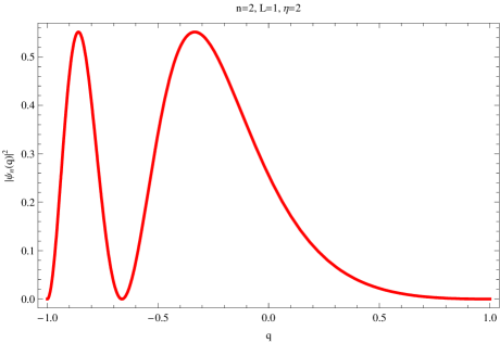
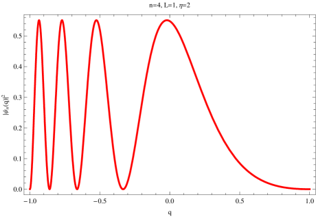
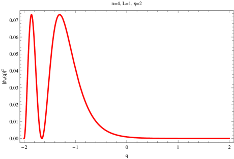
Figure 2: (Color online) $|\psi_{n}(q)|^{2}$ as a function of position for some values of $L$, $\eta$ and $n$ with $m=\hbar=1$.

At zero temperature all the levels are occupied up to the Fermi level, $\epsilon_{F}$; hence if we assume that the former are quasi-continuous kittel , then the density of states is equal to

$$dN=\frac{{8m^{9/2}}g}{\sqrt{2}\pi^{2}\hbar^{3}\eta^{3}}\sinh^{3}\Bigl{(}\eta L/m\Bigr{)}\sqrt{E}dE,$$ (88)

where $g$ denotes the degeneracy. Thus the total number of particles reads

$$N=\int\limits_{0}^{\epsilon_{F}}\frac{8{m^{9/2}}g}{\sqrt{2}\pi^{2}\hbar^{3}\eta^{3}}\sinh^{3}\Bigl{(}\eta L/m\Bigr{)}\sqrt{E}dE,$$ (89)

from which we find that

$$\epsilon_{F}=\frac{\hbar^{2}\eta^{2}}{8m^{3}}\sqrt[3]{\Biggl{(}\frac{6\pi^{2}N}{g}\Biggr{)}^{2}}\Biggl{/}\sinh^{2}\Bigl{(}\eta L/m\Bigr{)}.$$ (90)

This equality reveals that the Fermi energy gets smaller as $\eta$ increases, in accordance with relation (81). Now the total energy of the gas can be calculated using

$$E_{\rm tot}=\int\limits_{0}^{\epsilon_{F}}EdN,$$ (91)

which yields the familiar expression

$$E_{\rm tot}=\frac{3}{5}N\epsilon_{F}.$$ (92)

The fact that the total energy is still proportional to the Fermi energy explains the reason for which the pressure of the gas decreases due to the increase of $\eta$, as was found earlier via the classical partition function.

Actually, using the results of the previous section, together with pure classical arguments, we can explain this behavior as follows: For every particle the conservation law ($q\equiv x,y,z$)

$$\frac{d}{dt}(v_{q}{\rm e}^{-\eta q/m})=0,$$ (93)

holds at any moment in time. Hence, for $\eta>0$ and $q$ close to $L$, the velocity of the particle is quite large which means that it quickly leaves this region just after hitting the wall at $q=L$. On the contrary, the velocity is quite small in the neighborhood of $-L$: the particle is thus slowed down in this region, taking larger times to reach the wall at $q=-L$. Although the carried momentum is large near $q=L$, after sufficiently long time, there will be much more particles close to $-L$, as clearly indicated in figure 1; hence, as a whole, the pressure of the gas drops down.

At $T\neq 0$, the number of particles is given by

$$N=\frac{{8m^{9/2}}g}{\sqrt{2}\pi^{2}\hbar^{3}\eta^{3}}\sinh^{3}\Bigl{(}\eta L/m\Bigr{)}\int\limits_{0}^{\infty}\frac{\sqrt{E}dE}{1+\exp[(E-\mu)/k_{B}T]},$$ (94)

where $\mu$ denotes the chemical potential. By introducing the notation $z=\exp(\mu/k_{B}T)$, and making the change of variable $\xi=\exp(-E/k_{B}T)$, we can write

$$N=\frac{{8m^{9/2}}g}{\sqrt{2}\pi^{2}\hbar^{3}\eta^{3}}\sinh^{3}\Bigl{(}\eta L/m\Bigr{)}\Biggr{[}z(k_{B}T)^{3/2}i\int\limits_{0}^{1}\frac{\sqrt{\ln(\xi)}d\xi}{1+z\xi}\Biggr{]}.$$ (95)

Integrating by parts yields

$$N=-\frac{4m^{9/2}g(k_{B}T)^{3/2}}{\sqrt{2}\pi^{3/2}\hbar^{3}\eta^{3}}\sinh^{3}\Bigl{(}\eta L/m\Bigr{)}{\rm Li}_{\frac{3}{2}}\bigl{(}-{\rm e}^{\mu/k_{B}T}\bigr{)}.$$ (96)

Here, ${\rm Li}_{n}(x)$ is the polylogarithm function, defined by

$${\rm Li}_{n}(x)=\frac{(-1)^{n-1}}{\Gamma(n-2)}\int\limits_{0}^{1}\ln^{n-2}(y)\ln(1-xy)\frac{dy}{y}.$$ (97)

Then using equation (90) we find that the chemical potential is given in terms of the Fermi energy by

$$\mu=k_{B}T\ln\Biggl{\{}-{\rm Li}^{-1}_{\frac{3}{2}}\Bigg{[}-\frac{4}{3\sqrt{\pi}}\Biggl{(}\frac{\epsilon_{F}}{k_{B}T}\Biggr{)}^{3/2}\Biggr{]}\Biggl{\}},$$ (98)

where the superscript designates the inverse function. Similarly, the total energy of the gas at nonzero temperature is found to be equal to

$$E_{\rm tot} = -\frac{6m^{9/2}g(k_{B}T)^{5/2}}{\sqrt{2}\pi^{3/2}\hbar^{3}\eta^{3}}\sinh^{3}\Bigl{(}\eta L/m\Bigr{)}{\rm Li}_{\frac{5}{2}}\bigl{(}-{\rm e}^{\mu/k_{B}T}\bigr{)}.$$ (99)

$$= -\frac{9\sqrt{\pi}Nk_{B}T}{2}\Biggl{(}\frac{k_{B}T}{\epsilon_{F}}\Biggr{)}^{3/2}{\rm Li}_{\frac{5}{2}}\bigl{(}-{\rm e}^{\mu/k_{B}T}\bigr{)}.$$

Using the property poly

$$\frac{d}{dx}{\rm Li}_{n}(x)=\frac{{\rm Li}_{n-1}(x)}{x}$$ (100)

we find that the specific heat of the gas is

$$C_{V} = \Bigl{(}\frac{\partial E_{\rm tot}}{\partial T}\Bigl{)}_{V}$$ (101)

$$= -\frac{9\sqrt{\pi}N}{2}\Biggl{(}\frac{k_{B}T}{\epsilon_{F}}\Biggr{)}^{3/2}\Biggl{[}\frac{5k_{B}}{2}{\rm Li}_{\frac{5}{2}}\bigl{(}-{\rm e}^{\mu/k_{B}T}\bigr{)}+\frac{\mu}{T}{\rm Li}_{\frac{3}{2}}\bigl{(}-{\rm e}^{\mu/k_{B}T}\bigr{)}\Biggr{]}.$$

For $T\sim 0$ we may use the the approximations temp

$$\mu \approx \epsilon_{F}\Biggl{[}1-\frac{\pi^{2}}{12}\Biggl{(}\frac{k_{B}T}{\epsilon_{F}}\Biggl{)}^{2}\Biggr{]},$$ (102)

$$E_{\rm tot} \approx \frac{3}{5}N\epsilon_{F}\Biggl{[}1+\frac{5\pi^{2}}{12}\Biggl{(}\frac{k_{B}T}{\epsilon_{F}}\Biggl{)}^{2}\Biggr{]}.$$ (103)

This yields

$$C_{V}\approx\frac{1}{2}\pi^{2}Nk_{B}\frac{T}{\epsilon_{F}},$$ (104)

which implies that the specific heat of the gas increases with $\eta$.

IV Motion in the Morse potential

In this section we propose to solve the time-independent Schrödinger equation

$$\Biggl{[}-\frac{\hbar^{2}}{2m_{0}}\frac{1}{\sqrt{M(q)}}\frac{d}{dq}\frac{1}{\sqrt{M(q)}}\frac{d}{dq}+U(q;\alpha)-E\Biggr{]}\psi(q)=0$$ (105)

for the Morse potential morse

$$U(q;\alpha)=A({\rm e}^{-2\alpha q}-2{\rm e}^{-\alpha q}),\qquad A,\ \alpha>0.$$ (106)

We shall consider two special cases, namely, $M(q)=\exp\{\pm 2\eta q/m_{0}\}$, with

$$\eta/m_{0}=\alpha.$$ (107)

This choice leads to exact analytical solutions as we shall see bellow. Physically, the latter condition implies that the effective distance constant of the force (7) is equal to the effective range ($1/\alpha$ in lenght unit) of the Morse potential.

Consider first the case $M(q)=\exp\{2\eta q/m_{0}\}$, and let us look for the discrete spectrum corresponding to negative values of $E$. By virtue of equation (105), we can write

$$\frac{d^{2}\psi}{dq^{2}}-\frac{\eta}{m_{0}}\frac{d\psi}{dq}+\Biggl{[}\frac{2m_{0}E}{\hbar^{2}}{\rm e}^{2\eta q/m_{0}}-\frac{2m_{0}A}{\hbar^{2}}(1-2{\rm e}^{\eta q/m_{0}})\Biggr{]}\psi=0.$$ (108)

Making the change of variable

$$\xi=\frac{2\sqrt{-2m_{0}^{3}E}}{\hbar\eta}{\rm e}^{\eta q/m},$$ (109)

equation (108) becomes

$$\psi^{{}^{\prime\prime}}+\Biggl{[}-\frac{1}{4}+\Biggl{(}\frac{2m_{0}^{3}A}{\hbar\eta\sqrt{-2m_{0}^{3}E}}\Biggr{)}\frac{1}{\xi}-\Biggl{(}\frac{2m_{0}^{3}A}{\hbar^{2}\eta^{2}}\Biggr{)}\frac{1}{\xi^{2}}\Biggl{]}\psi=0.$$ (110)

We require that the function $\psi$ vanishes as $q\to\pm\infty$; in terms of the variable $\xi$, we have to study the behavior of $\psi$ at infinity and in the neighborhood of zero. One can show that

$$\psi \sim \xi^{(1+\sqrt{1+4s^{2}})/2}\quad{\text{as}}\quad\xi\to 0,$$ (111)

$$\psi \sim {\rm e}^{-\xi/2}\hskip 49.79231pt{\text{as}}\quad\xi\to\infty,$$ (112)

where we have introduced the quantity

$$s=\frac{\sqrt{2m_{0}^{3}A}}{\hbar\eta}.$$ (113)

Hence it is natural to seek a solution in the form

$$\psi(\xi)={\rm e}^{-\xi/2}\xi^{(1+\sqrt{1+4s^{2}})/2}\phi(\xi),$$ (114)

where $\phi$ is a new function of $\xi$. By direct substitution into (110), it can be verified that

$$\xi\phi^{{}^{\prime\prime}}+(1+\sqrt{1+4s^{2}}-\xi)\phi^{{}^{\prime}}+[\tau-(1+\sqrt{1+4s^{2}})/2]\phi=0,$$ (115)

with

$$\tau=\frac{2m_{0}^{3}A}{\hbar\eta\sqrt{-2m_{0}^{3}E}}.$$ (116)

Equation (115) is nothing but the differential equation associated with the confluent hypergeometric function abr ; poly

$$\phi=F(-n,2\kappa+1,\ \xi),$$ (117)

where

$$\kappa=\frac{1}{2}\sqrt{1+4s^{2}},\qquad n=\tau-\kappa.$$ (118)

It follows that the unnormalized eigenfunctions take the form

$$\psi_{n}(\xi)={\rm e}^{-\xi/2}\xi^{(1+\sqrt{1+4s^{2}})/2}F(-n,2\kappa+1,\ \xi).$$ (119)

The required conditions on the behavior of the wave function at $\pm\infty$ implies that only positive integer values of $n$ are allowed, whence

$$-E_{n}=\frac{2m_{0}^{3}A^{2}/\hbar^{2}\eta^{2}}{\Bigl{[}(n+\frac{1}{2})+\frac{1}{2}\sqrt{1+\frac{8m_{0}^{3}A}{\hbar^{2}\eta^{2}}}\Bigr{]}^{2}},\qquad n=n_{\rm min},\ n_{\rm min}+1,...$$ (120)

Here, $n_{\rm min}$ denotes the minimum positive integer number for which $-E<A$. Thus, although the spectrum of negative eigenvalues corresponding to the Morse potential consists of a finite number of levels for constant masses, the chosen form of the position dependence of the mass we have adopted above renders the number of energy levels infinite.

Now if we assume that $M(q)=\exp\{-2\eta q/m_{0}\}$, then we have that

$$\frac{d^{2}\psi}{dq^{2}}+\frac{\eta}{m_{0}}\frac{d\psi}{dq}+\Biggl{[}\frac{2m_{0}E}{\hbar^{2}}{\rm e}^{-2\eta q/m_{0}}-\frac{2m_{0}A}{\hbar^{2}}({\rm e}^{-4\eta q/m_{0}}-2{\rm e}^{-3\eta q/m_{0}})\Biggr{]}\psi=0.$$ (121)

By the change of variable

$$\xi={\rm e}^{-\eta q/m_{0}},$$ (122)

we get

$$-\frac{\hbar^{2}}{2m_{0}^{3}/\eta^{2}}\psi^{{}^{\prime\prime}}+A(\xi^{2}-2\xi)\psi=E\psi,$$ (123)

which is the differential equation for a parabolic cylinder function. Let us further introduce the notations

$$\omega^{2}=\frac{2A\eta^{2}}{m_{0}^{3}},\quad M=\frac{m_{0}^{3}}{\eta^{2}},\quad\mathcal{E}=E+A.$$ (124)

Hence with $\vartheta=1-\xi$, equation (123) takes the form

$$\Bigl{(}-\frac{\hbar^{2}}{2M}\frac{d^{2}}{d\vartheta^{2}}+\frac{1}{2}M\omega^{2}\vartheta^{2}\Bigr{)}\psi=\mathcal{E}\psi.$$ (125)

Clearly, the above procedure enables us to map the whole dynamics into a simple harmonic oscillator problem in the interval $]-\infty,1]$. It follows that the solution of (121) is

$$\psi_{n}(q)=C_{n}\exp\Biggl{\{}-\sqrt{\frac{m_{0}^{3}A}{2\hbar^{2}\eta^{2}}}\Bigl{(}1-{\rm e}^{-\eta q/m_{0}}\Bigr{)}^{2}\Biggr{\}}H_{n}\Biggl{[}\Bigl{(}1-{\rm e}^{-\eta q/m_{0}}\Bigr{)}\sqrt[4]{\frac{2m_{0}^{3}A}{\hbar\eta^{2}}}\Biggr{]},$$ (126)

with the eigenvalues

$$E_{n}=\hbar\sqrt{\frac{2A\eta^{2}}{m_{0}^{3}}}(n+\tfrac{1}{2})-A.$$ (127)

In the above, $C_{n}$ is a constant and $H_{n}(x)$ denotes Hermite’s polynomial of degree $n$; the allowed values of $n$ are those which satisfy the conditions

$$H_{n}\Bigl{(}\sqrt[4]{2m_{0}^{3}A/\hbar\eta^{2}}\Bigr{)}=0,\qquad-E_{n}<A.$$ (128)

The former equation can be solved either geometrically or numerically. Nevertheless, using the property

$$H_{2m+1}(0)=0,\qquad m=0,1,2,\cdots,$$ (129)

we conclude that for sufficiently large values of $\eta$, only odd values of $n$ should be taken into account, provided $-E_{n}<A$.

V Summary

Summing up, we have shown that the motion of position-dependent effective mass can be regarded as a damping-dantidamping dynamics of a constant mass under the effect of an effective potential, and vice versa. Care has to be taken when calculating the effective potentials since certain singularities may appear, which affects, in turn, the mass of the particle. We have quantized the equations of motions starting from a geometric interpretation of the motion; we found that it allows for a smooth transition to the constant-mass case, which does not hold for the momentum and mass ordering method. We have applied the obtained results to a Fermi gas of damped-antidamped particles. The classical and the quantum treatment of this system reveals that the pressure and the specific heat depend on the applied forces. Finally, by solving the Schrödinger equation in the presence of the Morse potential, we deduced the energy spectra and the eigenfunctions of the bound states in the case of a particle with exponentially decreasing or increasing mass. We found that the number of energy levels may become infinite for particular spatial dependence of the mass.

References

- (1) L. D. Landau and E. M. Lifshitz, Quantum Mechanics (Pergamon Press, London, 1965); P. A. M. Dirac, The Principles of Quantum Mechanics (Clarendon, Oxford, 1958); L. I. Schiff, Quantum Mechanics (McGraw-Hill, New York, 1949); A. Messiah, Quantum Mechanics, Vols. I and II (North-Holland, Amsterdam, 1961).
- (2) W. Greiner and J. A. Maruhn, Nuclear Models (Springer, Berlin, 1996).
- (3) C. Kittel, Introduction to Solid State Physics (John Wiley & Sons, New York, 1956).
- (4) L. Serra and E. Lipparini, Europhys. Lett. 40 667 (1997).
- (5) P. Harrison, Quantum Wells, Wires and Dots (John Wiley & Sons, New York, 2000).
- (6) G. Bastard, Wave Mechanics Applied to Semiconductor Hetero-structures (EDP Sciences, Les Editions de Physique, Les Ulis, France, 1992).
- (7) O. von Roos and H. Mavromatis, Phys. Rev. B 31 2294 (1985).
- (8) R. A. Morrow, Phys. Rev. B 35 8074 (1987).
- (9) W. Trzeciakowski, Phys. Rev. B 38 4322 (1988).
- (10) I. Galbraith and G. Duggan, Phys. Rev. B 38 10057 (1988).
- (11) K. Young, Phys. Rev. B 39 13434 (1989).
- (12) G. T. Einevoll, Phys. Rev. B 42 3497 (1990).
- (13) G.T. Einevoll, P.C. Hemmer, and J. Thomsen, Phys. Rev. B 42 3485 (1990).
- (14) A. Puente, Ll. Serra, and M. Casas, Z. Phys. D 31 283 (1994).
- (15) M. Barranco, M. Pi, S.M. Gatica, E.S. Hernandez, and J. Navarro, Phys. Rev. B 56 8997 (1997).
- (16) F. Arias de Saavedra, J. Boronat, A. Polls, and A. Fabrocini, Phys. Rev. B 50 4248 (1994).
- (17) L. Chetouani, L. Dekar, and T. F. Hammann, Phys. Rev. A 52 82 (1995).
- (18) L. Dekar, L. Chetouani, and T. F. Hammann, J. Math. Phys. 39 2551 (1998).
- (19) L. Dekar, L. Chetouani and T. F. Hammann, Phys. Rev. A 59 107 (1999).
- (20) A. R. Plastino, A. Puente, M. Casas, F. Garcias, and A. Plastino, Rev. Mex. Fis. 46 78 (2000).
- (21) R. Koç, M. Koca, and E. Körcük, J. Phys. A 35 L527 (2002).
- (22) B. Gönül, O. Özer, B. Gönül, and F. Üzgün, Mod. Phys. Lett. A 17 2453 (2002).
- (23) A. D. Alhaidari, Phys. Rev. A 66 042116 (2002).
- (24) A. de Souza Dutra and C. A. S. Almeida, Phys. Lett. A 275 25 (2000).
- (25) A. de Souza Dutra, M. Hott, and C. A. S. Almeida, Europhys. Lett. 62 8 (2003).
- (26) A. D. Alhaidari, Int. J. Theor. Phys. 42 2999 (2003).
- (27) J. Yu, S.-H.Dong, Phys. Lett.A 325 194 (2004).
- (28) J. Yu, S. H. Dong, and G. H. Sun, Phys. Lett. A 322 290 (2004).
- (29) A. G. M.Schmidt, Phys. Lett. A 353 459 (2006).
- (30) C. Quesne and V. M. Tkachuk, J. Phys. A: Math. Gen. 37 4267 (2004).
- (31) B. Bagchi, A. Banerjee, C. Quesne, and V. M. Tkachuk, J. Phys. A: Math. Gen. 38 2929 (2005).
- (32) C. Y. Cai, Z. Z. Ren, and G. X. Ju, Commun. Theor. Phys. 43 1019 (2005).
- (33) O. von Roos, Phys. Rev. B 27 7547 (1983).
- (34) L. D. Landau and E. M. Lifshitz, Mechanics (Pergamon, London, 1965).
- (35) U. Weiss, Quantum Dissipative Systems ( World Scientific, Singapore, 1993).
- (36) C. W. Gardiner, Quantum Noise (Springer, Berlin, 1991).
- (37) H. Hofmann, The Physics of Warm Nuclei (Oxford University Press, New York, 2008).
- (38) P. M. Morse, Phys. Rev. 34 57 (1929).
- (39) J. A. Kobussen, Act. Phys. Austr. 51 193 (1979).
- (40) C. C. Yan, Amer. J. Phys. 49 296 (1981).
- (41) C. Leubner, Phys. Rev. A 86 9 (1987).
- (42) G. López, Ann. Phys. 251 2 372 (1996).
- (43) M. Abramowitz and I. A. Stegun, Handbook of Mathematical Functions (Dover, New York, 1965).
- (44) G. E. Andews, R. Askey, and R. Roy, Special Functions (Cambridge University Press, Cambridge, 1999).
- (45) M. Toda, R. Kubo, and N. Saitô, Statistical Physics I, Equilibrium Statistical Mechanics (Springer, Berlin, Heidelberg, 1983).