General Relationship Between the Entanglement Spectrum and the Edge State Spectrum of Topological Quantum States

Abstract

We consider (2+1)-dimensional topological quantum states which possess edge states described by a chiral (1+1)-dimensional Conformal Field Theory (CFT), such as e.g. a general quantum Hall state. We demonstrate that for such states the reduced density matrix of a finite spatial region of the gapped topological state is a thermal density matrix of the chiral edge state CFT which would appear at the spatial boundary of that region. We obtain this result by applying a physical instantaneous cut to the gapped system, and by viewing the cutting process as a sudden “quantum quench” into a CFT, using the tools of boundary conformal field theory. We thus provide a demonstration of the observation made by Li and Haldane about the relationship between the entanglement spectrum and the spectrum of a physical edge state.

Topological phases of matter are gapped quantum states which cannot be adiabatically deformed into a completely ‘trivial’ gapped system such as a trivial band insulator, without crossing a quantum phase transition. They are not characterized by symmetry breaking, but instead by certain global topological properties such as the presence of (topologically) protected edge states and/or a ground state degeneracy which depends on the topology of the surface on which the state residesWen and Niu (1990). Topological states of matter of this kind which have been discovered in nature include the integer and fractional quantum Hall statesedited by R. E. Prange and Girvin (1987), and the recently discovered time-reversal invariant topological insulatorsHasan and Kane (2010); Qi and Zhang (2010); Moore (2009).

Quantum entanglement is a purely quantum mechanical phenomenon which has no classical analog. For any pure quantum state (typically the ground state) of a system consisting of two disjoint subsystems $A$ and $B$, subsystem $A$ can be described by a density matrix obtained by ‘tracing out’ the degrees of freedom in $B$. This density matrix provides complete information about the entanglement properties of the initial pure state between the two subsystems. Quantum entanglement provides an alternative characterization of the properties of the many-body system, in particular for topological states of matter which cannot be described by conventional probes such as order parameters, correlation functions, etc.. Amico et al. (2008) For example, as discovered by Levin and Wen, and by Kitaev and PreskillLevin and Wen (2006); Kitaev and Preskill (2006), the entanglement entropy of a topologically ordered state in a region of linear size $l$ in two-dimensional position space contains a universal $l$-independent term, the ‘topological entanglement entropy’ (TEE), which is a characteristic of the topological order of the state. However, the TEE is not a complete description of a topological state of matter, since distinct topologically ordered states can have the same TEE. More complete information about a topological state of matter can be obtained from the eigenvalue spectrum of the reduced density matrix, often referred to as the entanglement spectrumLi and Haldane (2008). In general, the density matrix $\rho_{A}$ describing the entanglement between a subsystem $A$ and the rest of the system can be written in the form of $\rho_{A}=e^{-H_{\rm E}}$, with $H_{\rm E}$ a Hermitian operator. This is so far nothing but the definition of $H_{\rm E}$. In general, the so-defined “entanglement Hamiltonian” $H_{\rm E}$ is different from the physical Hamiltonian of the system. (In this form, the operator $H_{\rm E}$ appears formally in a way analogous to that of the physical Hamiltonian $\beta H$ in a system in thermal equilibrium, which has a thermal density matrix $\rho\propto e^{-\beta H}$ at temperature $T=1/k_{\rm B}\beta$.) One important physical feature of the so-defined entanglement Hamiltonian $H_{E}$ is that its low-energy eigenstates correspond to those states in subsystem $A$, appearing in the Schmidt-decomposition of the initial pure state, which are most entangled with the rest of the system.

The focus of the present article is a remarkable observation made recently by Li and HaldaneLi and Haldane (2008) and in subsequent work for topological phases whose physical Hamiltonian possesses low energy states at an open boundary (‘edge states’). This includes fractional quantum Hall statesLi and Haldane (2008); Läuchli et al. (2010); Regnault et al. (2009); Thomale et al. (2010), non-interacting topological insulatorsTurner et al. (2010); Fidkowski (2010a) and the Kitaev honeycomb modelYao and Qi (2010). It was found that for those systems the low-energy ‘edge’ states of the physical Hamiltonian at an actual open boundary of system A are in one-to-one correspondence with the low-lying eigenstates of entanglement Hamiltonian $H_{\rm E}$ (i.e. with the most entangled states). However, except for systems which can be reduced to non-interacting fermion problemsTurner et al. (2010); Fidkowski (2010b); Yao and Qi (2010), such a correspondence between entanglement spectrum and the edge state spectrum of the physical Hamiltonian has only been supported by numerical evidence. No general argument for the validity of such a correspondence has been presented so far. It is the purpose of the present Letter to demonstrate the general validity of this correspondence.

General setup– In this Letter, we show that for a generic $(2+1)$-dimensional topological state which possesses edges states described by a conformal field theory, the entanglement Hamiltonian $H_{\rm E}$ is proportional to the Hamiltonian $H_{L}$ of a physical chiral (say L-moving) edge state appearing an actual spatial boundary of subsystem A, in the long-wavelegnth limit and in any fixed topological sector. For example, our conclusion applies to all the Abelian and non-Abelian quantum Hall states described by Chern-Simons effective field theories in the bulkZhang et al. (1989); Blok and Wen (1990); Witten (1989); Moore and Read (1991). In order to relate the entanglement spectrum and spectrum of the physical edge state Hamiltonian, we consider a bipartition of the toplogical state on a cylinder into two parts $A$ and $B$ as shown in Fig. 1 (a). The (physical) Hamiltonian $H$ can be written in the form

$$H=H_{A}+H_{B}+H_{AB}$$ (1)

where $H_{A}$ and $H_{B}$ denote the Hamiltonians in disconnected regions $A$ and $B$, respectively, each of which has (two) open boundaries. The term $H_{AB}$ couples regions $A$ and $B$ across their joint boundary. For example, for a 2D gapped tight-binding model $H=\sum_{\left\langle ij\right\rangle}c_{i}^{\dagger}t_{ij}c_{j}$ realizingHaldane (1988) the integer quantum Hall effect, the term $H_{AB}$ contains all the electron hopping terms across the boundary between $A$ and $B$.

Now we consider a deformed Hamiltonian containing a parameter $\lambda\in[0,1]$ (similar to Ref. Qi et al. (2006)):

$$H(\lambda)=H_{A}+H_{B}+\lambda H_{AB}$$ (2)

By construction, $H(\lambda=0)$ is the Hamiltonian of the two decoupled cylinders $A$ and $B$, and $H(\lambda=1)$ is the Hamiltonian of the whole cylinder $A\cup B$. Since we are interested in such topological states which possess chiral edge states, the Hamiltonian $H(\lambda=0)$ will have chiral and anti-chiral edge states propagating at the boundary between regions $A$ and $B$, as shown in Fig. 1 (b). When $\lambda\neq 0$, the term $\lambda H_{AB}$ introduces a coupling between the regions $A$ and $B$. Denote the bulk gap of the Hamiltonian $H=H(\lambda=1)$ by $E_{\rm g}$. When the coupling $\lambda$ is small enough such that the energy scale of the coupling term $\lambda H_{AB}$ is much smaller than the bulk gap $E_{\rm g}$, the gapped bulk states described by $H_{A}$ and $H_{B}$ are almost entirely unaffected by the coupling term $\lambda H_{AB}$, whose main effect is then to induce an inter-edge coupling between the chiral and anti-chiral edge states. Since each individual edge state is described by a chiral conformal field theory (CFT), the theory of the two edges between regions $A$ and $B$ is described by a non-chiral conformal field theory. Thus at low-energy the coupling term $\lambda H_{AB}$ between regions $A$ and $B$ is reduced to a local interaction in the CFT describing the dynamics of the two coupled edges. If this interaction is a relevant perturbation of the CFT describing the decoupled edges, then the two counterpropagating edges will be gapped for arbitrarily small coupling $\lambda$. Thus we expect that in this case the system described by the Hamiltonian $H(\lambda=1)$ to be adiabatically connected to that described by $H(\lambda)$ for a small but non-vanishing value of $\lambda$. In this case, the entanglement properties of $H(\lambda=1)$ are expected to be qualitatively the same as those of $H(\lambda)$ with a small $\lambda$. The latter describes the entanglement between the left- and the right-movers of the edge state CFT. Let us assume for simplicity that this coupling is relevant in the renormalization group (RG) sense.

Below we will solve this entanglement problem for the edge state CFT, by mapping it to a problem of a quantum quench. We then solve the latter (quantum quench) problem in the standard manner by using the work of Calabrese and CardyCalabrese and Cardy (2006, 2007) which employs the methods of boundary conformal field theory (BCFT)Cardy (1989).

Reduced density matrix of the edge CFT– Next we study the entanglement properties of the Hamiltonian $H(\lambda)$ for small values of $\lambda$, which, as explained above, amounts to the study of the $(1+1)$ dimensional problem of coupled edge states,

$$H_{\rm edge}(\lambda)=H_{L}+H_{R}+\lambda H_{\rm int}$$ (3)

Here, $H_{L}$ and $H_{R}$ denote the Hamiltonians of left-moving (L) and right-moving (R) edge states, and $\lambda H_{\rm int}$ a relevant inter-edge coupling. The left- and right- moving edge states are the low-energy excitations of the subsystem in regions $A$ and $B$, respectively. Again, the entanglement properties between the subsystems $A$ and $B$ are reduced to those between left and right moving $(1+1)$-dimensional edge states. If we denote the ground state of the Hamiltonian $H_{\rm edge}(\lambda)$ from Eq.(3) by $G$, then our goal is to obtain the density matrix of the left-moving edge state subsystem defined by

$$\rho_{L}={\rm Tr}_{R}\left(\left|G\right\rangle\left\langle G\right|\right),$$ (4)

where ${\rm Tr}_{R}$ denotes the trace over the right-moving edge state degrees of freedom. In general, the ground state $\left|G\right\rangle$ will depend on all the details of the coupling between the right- and the left- moving edges states. However, due to the gapless nature of $H_{\rm edge}(\lambda=0)$ describing the decoupled edges, certain universal properties can be inferred without reference to any detailed features of this coupling in the long-wavelength limit.

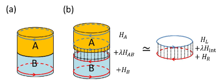
Figure 1: (a) A topological state on a cylinder with a bipartition into two regions $A$ and $B$. (b) The deformed system (see text) with the coupling between $A$ and $B$ regions weighted by a factor $\lambda\in[0,1]$. The system can be understood as two cylinders $A$ and $B$, with edge states propagating along the boundary between $A$ and $B$, coupled by an inter-edge coupling. (c) For small enough $\lambda$, the coupling between the gapped bulk states can be neglected, and the problem can be reduced to an inter-edge coupling problem described by a $(1+1)$-dimensional conformal field theory with a relevant coupling $\lambda H_{\rm int}$.

In order to understand the entanglement properties of the state $\left|G\right\rangle$, we relate them to another problem – the “quantum quench” problem. Consider a “quantum quench” of the system composed of the coupled edges, Eq. 3. For all times $t<0$ the system is in the ground state $\left|G\right\rangle$ of the Hamiltonian $H_{edge}(\lambda_{0})$ with non-vanishing coupling $\lambda_{0}\not=0$ between the edges. At time $t=0$ the coupling $\lambda_{0}$ between the edges is suddenly switched off, so that $\lambda=0$ for $t\geq 0$. After the quantum quench, the left and right moving edge states evolve independently with the Hamiltonian $H_{\rm edge}(\lambda=0)=$ $H_{L}+H_{R}$ of the decoupled edges. Space- and time-dependent correlation functions after a sudden quench, as above, have been studied extensively by Calabrese and CardyCalabrese and Cardy (2006, 2007), who applied BCFT to obtain general properties of such correlation function in the long-time and long-wavelength regime. This is relevant for our purpose because the density matrix $\rho_{L}$ is uniquely determined by the set of all the equal-time correlation functions of operators with support solely on the left-moving edge,

$$C(t,\left\{x_{i}\right\})=$$

$$\left\langle G\right|e^{it(H_{L}+H_{R})}\hat{O}_{L,1}(x_{1})...\hat{O}_{L,n}(x_{n})e^{-it(H_{L}+H_{R})}\left|G\right\rangle\equiv$$

$$\equiv{\rm Tr}_{L}\left[e^{-itH_{L}}\rho_{L}e^{itH_{L}}\hat{O}_{L,1}(x_{1})...\hat{O}_{L,n}(x_{n})\right],$$ (5)

(All the coordinates $x_{1},x_{2},...x_{n}$ reside entirely on the left-moving edge.) In the quantum quench problem, the ground state $\left|G\right\rangle$ of the coupled edge Hamiltonian $H_{edge}(\lambda_{0}\not=0)$ represents an initial condition at time $t=0$ for the evolution with the gapless (critical) decoupled edge system Hamiltonian $H_{L}+H_{R}$ at subsequent times $t>0$. This initial state can be viewedSymanzik (1981); Calabrese and Cardy (2006, 2007) as a boundary condition on the gapless theory of the right and left moving edges. It can thus be described using the methods of boundary critical phenomenadie . This can be achieved in any dimension of space by analytical continuation of the real-time Keldysh contour to imaginary time, and subsequent exchange of the roles of space and imaginary time (possible due to the underlying effective relativistic invariance of the low-energy edge state theory). Moreover, in the present case of a one-dimensional edge, the resulting boundary condition can be analyzed by using the powerful tools of BCFTCardy (1989). The key result that we will use from the theory of boundary critical phenomena is that an arbitrary boundary condition on a gapless bulk theory will always renormalize at long distances into a scale invariant boundary conditionAffleck and Ludwig (1991); see e.g. A. W. W. Ludwig (1994); Calabrese and Cardy (2006). Moreover, in the case of a (1+1) conformal bulk theory, such as the one describing the one-dimensional edges, any scale invariant boundary conditions must be one of a known list of conformally invariant boundary conditionsCardy (1989). Consequently, as emphasized in Ref. Calabrese and Cardy (2006), in the long wavelength limit the correlation functions at a general boundary condition described by a general state $\left|G\right\rangle$ are equal to those at a conformally invariant boundary condition described by a state $\left|G_{*}\right\rangle$ which represents a (boundary) fixed point to which the boundary state $\left|G\right\rangle$ flows under the renormalization group (RG). The difference between $\left|G\right\rangle$ and $\left|G_{*}\right\rangle$ can be represented by an imaginary time evolution operator,

$$\left|G\right\rangle\simeq Z^{-1/2}e^{-\tau_{0}(H_{L}+H_{R})}\left|G_{*}\right\rangle$$ (6)

where $\tau_{0}>0$ is the so-called extrapolation lengthCalabrese and Cardy (2006); die and stands for the RG “distance” of the general boundary state $\left|G\right\rangle$ to the conformal boundary state $\left|G_{*}\right\rangle$. $Z=\left\langle G_{*}\right|e^{-2\tau_{0}(H_{L}+H_{R})}\left|G_{*}\right\rangle$ is a nomalization factor. Physically, the energy scale $1/\tau_{0}$ is determined by the energy gap $E(\lambda_{0})$ induced by the coupling term $\lambda_{0}H_{\rm int}$ between the edges.

In a so-called rational CFT such as the one under consideration, all conformal invariant boundary states $\left|G_{*}\right\rangle$ are knownCardy (1989) to be finite linear combinations of so-called Ishibashi statesIshibashi (1989) which have the form

$$\left|G_{*,a}\right\rangle=$$

$$=\sum_{n=0}^{\infty}\sum_{j=1}^{d_{a}(n)}\left|k(a,n),j;a\right\rangle_{L}\otimes\left|-k(a,n),j;\bar{a}\right\rangle_{R}.$$ (7)

Here $a$ denotes a topological sector in the underlying topological theory, i.e. a topological flux threading the cylinder in Fig. (1(a)), which is represented in the CFT describing the edges by a primary state of a corresponding conformal symmetry algebra (Virasoro or other) of conformal weight $h_{a}$. ($\bar{a}$ denotes the conjugate sector and state of conformal weight $h_{\bar{a}}=h_{a}$.) The label $a$ runs over all possible particle types of the topological state Moore and Seiberg (1989). Here $k(a,n)=2\pi(h_{a}+n)/l$ denotes the momentum, where where $l$ is the circumference of the edge of the cylinder; $j=1,2,..d_{a}(n)$ labels the elements of an orthonormal basis in the subspace of fixed momentum $k(a,n)$. Notice that the left- (right-) moving edge system only contains excitations with positive (negative) momentum. We note that the state in Eq. 7 is and example of a so-called maximally entangled state. The explicit form, Eq. 7, of the Ishibashi states $\left|G_{*,a}\right\rangle$, resulting from conformal invariance, is of great help in determining the form of the reduced density matrix $\rho_{L}$ for the left-moving edge. Upon directly combining Eqs. (6) with (7) one obtains

$$\left|G_{a}\right\rangle\simeq$$

$$\simeq\sum_{n=0}^{\infty}{e^{-2\tau_{0}vk(a,n)}\over Z^{1/2}}\sum_{j=1}^{d_{a}(n)}\left|k(a,n),j;a\right\rangle_{L}\otimes\left|-k(a,n),j;\bar{a}\right\rangle_{R}$$

which yields the following form of the density matrix of the left-moving edge upon tracing out the right moving edge,

$$\rho_{La}={\rm Tr}_{R}\left(\left|G_{a}\right\rangle\left\langle G_{a}\right|\right)\simeq$$

$$\simeq\sum_{n=0}^{\infty}{e^{-4\tau_{0}vk(a,n)}\over Z}\sum_{j=1}^{d_{a}(n)}\left|k(a,n),j;a\right\rangle_{L}\left\langle k(a,n),j;a\right|_{L}=$$

$$=Z^{-1}{\hat{P}}_{a}\ e^{-4\tau_{0}H_{L}}{\hat{P}}_{a}$$ (8)

Here we have used the linear dispersion $H_{L}\left|k,j;a\right\rangle_{L}=vk(a,n)\left|k,j;a\right\rangle_{L}$, $H_{R}\left|-k,j;\bar{a}\right\rangle_{L}=vk\left|-k,j;\bar{a}\right\rangle_{R}$ where $v$ is the edge state velocity and $k$ stands for $k(a,n)$. The label $a$ indicates that $\rho_{La}$ is an operator defined in the topological sector corresponding to topological flux $a$ threading the cylinder, and ${\hat{P}}_{a}$ is the projection operator onto that sector of the Hilbert space of the CFT. In cylinder geometry there is no entanglement between different topological sectors (denoted by different labels $a$).

Eq. (8) is the central result of this work, which demonstrates that the entanglement between left-moving and right-moving edge states in a CFT induced by a relevant coupling is always characterized by a “thermal” density matrix within a fixed topological sector (or primary state, in the CFT context). In other words, in each topological sector the “entanglement Hamiltonian” $H_{\rm E}=-\log\rho_{L}=4\tau_{0}H_{L}+\log Z$ is proportional to the Hamiltonian $H_{L}$ of a physical edge up to a possible shift of the ground state energy in that sector which ensures the proper normalization of the density matrix as a probability distribution. Our result demonstrates not only that the excitation energies of the entanglement spectrum are the same as those of the spectrum of the Hamiltonian of the edge state of the topological system appearing (by assumption) at a physical boundary of region A, in the long-wavelength limit modulo a global rescaling, but also that the most entangled states are in one-to-one correspondence with the low-energy edge states which occur at this boundary.

Example: Free fermions– A simple example in which the general notions, developed in the preceeding part of this article, can also be illustrated using elementary many-body techniques is that of the 2D integer quantum Hall (IQH) state (and more generally non-interacting topological insulators). This state can be described by a free fermion theory, the entanglement properties of which have been studied extensively in the literaturePeschel (2003); Turner et al. (2010); Fidkowski (2010b). However, it is still helpful to present the results here as an illustration, in the language of the much more general formulation obtained above. The edge states of an IQH state with integer filling fraction $\nu=N$ consist of $N$ flavors of non-interacting chiral fermions. For simplicity, we consider an IQH state with filling fraction $N=1$, whose edge state dynamics is governed by the Hamiltonian

$$H_{L}=\sum_{k}vkc_{k}^{\dagger}c_{k},~{}H_{R}=-\sum_{k}vkd_{k}^{\dagger}d_{k}$$ (9)

The simplest inter-edge coupling term is a single-particle inter-edge tunneling

$$H_{\rm int}=E_{\rm g}\sum_{k}\left(c_{k}^{\dagger}d_{k}+d_{k}^{\dagger}c_{k}\right)$$ (10)

with $E_{\rm g}$ the bulk gap which acts as a high-energy cut-off scale for the edge theory. The coupled Hamiltonian $H_{L}+H_{R}+\lambda H_{\rm int}$ is a free Fermion Hamiltonian which can be diagonalized by a unitary transformation to $H_{L}+H_{R}+H_{\rm int}=\sum_{k,s=\pm 1}E_{k}\gamma_{ks}^{\dagger}\gamma_{ks}$ with the gapful energy dispersion $E_{k}=\sqrt{v^{2}k^{2}+E_{\rm g}^{2}}$. Here $\gamma_{k,i}$ ($i=1,2$) are quasiparticle annihilation operators. The ground state $\left|G\right\rangle$ of this gapped system is determined by the conditions $\gamma_{k,i}\left|G\right\rangle=0$ ($i=1,2$). One obtains the following explicit expression for $\left|G\right\rangle$ (unnormalized):

$$\left|G\right\rangle = e^{-H_{\rm e}}\left|G_{*}\right\rangle$$ (11)

with

$$\left|G_{*}\right\rangle = \exp\left\{-\sum_{k>0}\left(c_{k}^{\dagger}d_{k}+d_{-k}^{\dagger}c_{-k}\right)\right\}\left|G_{L}\right\rangle\otimes\left|G_{R}\right\rangle.$$

and $H_{e}\simeq\frac{1}{2E_{\rm g}}(H_{L}+H_{R})$ in the long wavelength limit. The operators $c^{\dagger}_{k}d_{k}$ and $d^{\dagger}_{-k}c_{-k}$ with $k>0$ create quasiparticle excitations of the system of the two edges, so that $\left|G_{*}\right\rangle$ is an equal-weight superposition of all quasi-particle excitation states in the massless theory; this is nothing but the Ishibashi state for the Free fermion CFT (in the sector without topological flux). Thus, with this form of $H_{e}$, we recover correctly (in the long wavelength limit) the general relation (6); the extrapolation length is $\tau_{0}=1/2E_{\rm g}$. As expected, the energy scale $1/\tau_{0}$ is determined by the energy gap $2E_{\rm g}$ of particle-hole excitations.

Conclusion and discussion– In conclusion, we have demonstrated that for a generic $(2+1)$ dimensional topological state possessing gapless edge states which are described by a chiral CFT, the reduced density matrix of of a region $A$ obtained by tracing out the rest of the system always has, in the long wavelength limit, the same form as a thermal density matrix of region $A$ with an open physical boundary. Besides topological states, our analysis also applies to other systems described by coupled CFTs. In particular, our result provides an explanation of the recent numerical and analytical results on the entanglement spectrum of coupled spin chainsPoilblanc (2010) and coupled Luttinger liquidsFurukawa and Kim (2011). Since the relationship between a general boundary state and a scale invariant boundary condition which is the endpoint of the RG flow also holds for higher dimensional scale invariant bulk theoriesdie , we expect that our result will generalize to higher dimensional topological states, such as $(3+1)$ dimensional topological insulators, and especially the fractional topological insulators Levin and Stern (2009); Maciejko et al. (2010); Swingle et al. (2010); Cho and Moore which cannot be analysed using free fermion methodsTurner et al. (2010); Fidkowski (2010b). Details of this generalization will be left for future work.

We would like to note that the reduced density matrix (8) in the topological sector $a$ yields an entanglement entropy of the form $S=-{\rm Tr}\left(\rho_{L}\log\rho_{L}\right)=\alpha L-S_{\rm topo}$, with $S_{\rm topo}=\log\left(D/d_{a}\right)$ the topological entanglement entropyLevin and Wen (2006); Kitaev and Preskill (2006). Here $d_{a}$ is the quantum dimension of the quasi-particle of type $a$, and $D=\sqrt{\sum_{a}d_{a}^{2}}$ is the total quantum dimension. This relation to the topological entropy has been noticed in Ref. Kitaev and Preskill (2006), though in that work the form (8) of the density matrix was taken as an assumption. The present paper proves this assumption.

HK was supported in part by the National Science Foundation under Grant No. PHY05-51164 and JSPS. This work was supported, in part, by the NSF under Grant No. DMR- 0706140 (A.W.W.L.), Alfred P. Sloan Foundation (X.L.Q.).

Appendix A Supplentary Material I: More detailed discussion on irrelevant inter-edge coupling

In the main text we have mainly studied the cases in which the interaction term $\lambda H_{\rm int}$ in Eq. (3) is a relevant coupling in the edge CFT, so that a gap is induced once a finite coupling $\lambda\neq 0$ is turned on. In this appendix, we will discuss the cases in which the interaction term $\lambda H_{\rm int}$ is irrelevant, and provide arguments that our result on entanglement spectrum still holds in this case.

For concreteness of the discussion, we study the simplest fractional quantum Hall state–$1/m$ Laughlin state as an example. In the cylinder geometry shown in Fig. 1, the two edges in the middle are described by a Luttinger liquid (see e.g. Wen (1995))

$$\mathcal{L}_{0}=\frac{m}{2\pi}\left(\partial_{t}-v\partial_{x}\right)\phi_{L}\partial_{x}\phi_{L}+\frac{m}{2\pi}\left(-\partial_{t}-v\partial_{x}\right)\phi_{R}\partial_{x}\phi_{R}$$ (13)

The inter-edge interaction can be written asMoon et al. (1993)

$$\mathcal{L}_{\rm int} = \lambda\cos\left[\frac{1}{R}(\phi_{L}-\phi_{R})\right]$$ (14)

Physically, electron inter-edge tunneling corresponds to $R=1$. When a forward scattering term such as $g\partial_{\mu}\phi_{L}\partial^{\mu}\phi_{R}$ is turned on together with the back-scattering term, the compactification radius $R$ can deviate from $1$. For fractional quantum Hall edge states $m>1$ is an odd integer, and the coupling $\lambda$ is irrelevant if $R=1$, as shown in Fig. 2. If $\lambda$ is continuously tuned starting from $\lambda=0$, the system remains gapless until $\lambda=\lambda_{c}$ where a phase transition occurs and the system becomes gapped. By construction, the physical system (Fig. 1 (a)) without edge between A and B region corresponds to some value $\lambda>\lambda_{c}$ in the gapped phase, as shown in Fig. 2 by point A. For $\lambda<\lambda_{c}$ the coupling is irrelevant, but the compactification radius $R$ of the theory is renormalized. In other words, for $\lambda<\lambda_{c}$ the long wavelength behavior of the coupled system is still described by a CFT but it is different from the original CFT in Eq.(13). Thus naively it seems that our derivation in the main text does not directly apply to this theory. However, if we also turn on the forward scattering which increases $R$, the scaling dimension of $\lambda$ can be tuned to the region where $\lambda$ is relevant, as shown in Fig. 2 by point B. At this point Eq. (8) applies, and the reduced density matrix can be written as $\rho_{L}=Z^{-1}e^{-4\tau_{0}H_{L}}$ in each given topological sector. Now consider a path in the parameter space connecting A and B parameterized by $(\lambda(t),R(t))$ with $t\in[0,1]$. As long as the path stays in the gapped phase, for each point on the path the system has a gapped ground state $\left|G(\lambda(t),R(t))\right\rangle$, which determines a reduced density matrix $\rho_{L}(\lambda(t),R(t))={\rm Tr}_{R}\left|G(\lambda(t),R(t))\right\rangle\left\langle G(\lambda(t),R(t))\right|$ correspondingly. Since no phase transition occurs along the path, the wavefunction of the state $\left|G(\lambda(t),R(t))\right\rangle$ is a smooth function of $\lambda$ and $R$, so that $\rho_{L}(\lambda(t),R(t))$ is also smooth. Consequently, there is a one-to-one correspondence between the states in the low-lying entanglement spectrum of $\rho_{L}$ at the two points A and B. In other words, the low-lying entanglement spectrum of point A contains the same states as the chiral CFT of the edge theory. The eigenvalues of $H_{E}=-\log\rho_{L}(\lambda(t),R(t))$ can change continuously during the deformation, but the long-wavelength limit of the dispersion relation has to remain linear since the deformation is smooth. Thus in the long wavelength limit, the reduced density matrix $\rho_{L}$ at A point still has the form of Eq. (8), with generically a different $\tau_{0}$ from B point.

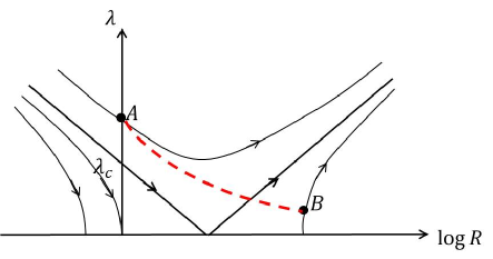
Figure 2: Illustration of the RG flow of model (13) and (14) with two parameters $\lambda$ and $R$. Any two points A and B in the gapped phase can be connected by a continuous path (red dash line). By this continuous deformation one can show that the entanglement spectrum of system A is qualitatively the same as system B. The entanglement Hamiltonian of system B can be obtained using the approach in the main text since $\lambda$ is relevant.

The argument above applies to more generic CFTs as long as such path in the parameter space of the theory exists, which smoothly connects the parameter region where the coupling is irrelevant to the region where the coupling is relevant. In other words, when the coupling $\lambda H_{\rm int}$ is irrelevant, our conclusion on the relation between entanglement spectrum and edge state spectrum still holds as long as there is a marginal coupling in the CFT which can tune the scaling dimension of $H_{\rm int}$ continuously to make it relevant.

Appendix B Supplementary Material II: Detailed derivation of the free Fermion density matrix

The free fermion Hamiltonian given by Eq. (9) and (10) can be diagonalized in the following form:

$$H_{L}+H_{R}+\lambda H_{\rm int} = \sum_{k,s=\pm 1}E_{k}\gamma_{ks}^{\dagger}\gamma_{ks}$$ (15)

$$\text{with~{}}E_{k} = \sqrt{v^{2}k^{2}+E_{\rm g}^{2}},~{}\left(\begin{array}[]{c}\gamma_{k+}\\ \gamma_{-k,-}^{\dagger}\end{array}\right)=\left(\begin{array}[]{cc}u_{k}&-v_{k}\\ v_{k}&u_{k}\end{array}\right)\left(\begin{array}[]{c}c_{k}\\ d_{k}\end{array}\right),~{}\left(\begin{array}[]{c}u_{k}\\ v_{k}\end{array}\right)=\left(\begin{array}[]{c}\sqrt{\frac{E_{k}+vk}{2E_{k}}}\\ -\sqrt{\frac{E_{k}-vk}{2E_{k}}}\end{array}\right)$$ (26)

The ground state $\left|G\right\rangle$ of this gapped system can be determined by the conditions $\gamma_{ks}\left|G\right\rangle=0$ for $s=\pm 1$, which leads to the following form (not normalized)

$$\left|G\right\rangle = \exp\left\{\sum_{k>0}\frac{v_{k}}{u_{k}}c_{k}^{\dagger}d_{k}+\sum_{k<0}\frac{u_{k}}{v_{k}}d_{k}^{\dagger}c_{k}\right\}\left|G_{L}\right\rangle\otimes\left|G_{R}\right\rangle$$

with $\left|G_{L(R)}\right\rangle$ the ground states of the gapless systems $H_{L}$ and $H_{R}$, respectively. The operators $c_{k}^{\dagger}d_{k}$ and $d_{k}^{\dagger}c_{k}$ creates particle-hole excitations in the massless theory. The physical meaning of this state can be understood better by redefining the quasi-particle creation operators in the massless theory as $L_{1k}=c_{k}$ and $L_{2k}=c_{-k}^{\dagger}$ for $k>0$, and similarly $R_{1k}=-d_{-k}^{\dagger}$ and $R_{2k}=d_{k}$ for $k<0$. In term of these operators,

$$\left|G\right\rangle = \exp\left\{\sum_{k>0}\frac{E_{\rm g}}{E_{k}+vk}\Delta_{k}^{\dagger}\right\}\left|G_{L}\right\rangle\otimes\left|G_{R}\right\rangle$$ (28)

with

$$\Delta_{k}^{\dagger}=L_{k1}^{\dagger}R_{-k1}^{\dagger}+L_{k2}^{\dagger}R_{-k2}^{\dagger}=-\left(c_{k}^{\dagger}d_{k}+d_{-k}^{\dagger}c_{-k}\right)$$ (29)

creates a pair of quasi-particles in the two edges. Defining

$$H_{e} = -\frac{1}{2}\sum_{k>0,s=1,2}\log\left({\frac{E_{\rm g}}{E_{k}+vk}}\right)\left(L_{ks}^{\dagger}L_{ks}+R_{-k,s}^{\dagger}R_{-k,s}\right)$$ (30)

$$= -\frac{1}{2}\sum_{k>0,s=1,2}\log\left({\frac{E_{\rm g}}{E_{k}+vk}}\right)\left(c_{k}^{\dagger}c_{k}-d_{k}^{\dagger}d_{k}+c_{-k}c_{-k}^{\dagger}-d_{-k}d_{-k}^{\dagger}\right)$$

we have the identity

$$e^{-H_{e}}L_{ks}^{\dagger}e^{-H_{e}}=\sqrt{\frac{E_{\rm g}}{E_{k}+vk}}L_{ks}^{\dagger},~{}e^{-H_{e}}R_{ks}^{\dagger}e^{-H_{e}}=\sqrt{\frac{E_{\rm g}}{E_{k}+vk}}R_{ks}^{\dagger}$$ (31)

Consequently $\left|G\right\rangle$ can be rewritten as

$$\left|G\right\rangle = e^{-H_{e}}\exp\left\{\sum_{k>0}\Delta_{k}^{\dagger}\right\}e^{-H_{e}}\left|G_{L}\right\rangle\otimes\left|G_{R}\right\rangle$$ (32)

$$= e^{-H_{e}}\exp\left\{\sum_{k>0}\Delta_{k}^{\dagger}\right\}\left|G_{L}\right\rangle\otimes\left|G_{R}\right\rangle\equiv e^{-H_{e}}\left|G_{*}\right\rangle$$

In the last line, we have used the fact that $H_{e}\left|G_{L}\right\rangle\otimes\left|G_{R}\right\rangle=0$. In the long-wavelength limit $k\rightarrow 0$, $H_{e}$ in Eq. (30) is expanded as

$$H_{e} \simeq \sum_{k>0,s=1,2}\frac{vk}{2E_{\rm g}}\left(L_{ks}^{\dagger}L_{ks}+R_{-k,s}^{\dagger}R_{-k,s}\right)$$ (33)

$$\equiv \frac{1}{2E_{\rm g}}\left(H_{L}+H_{R}\right)$$

Consequently, Eq. (32) in the long wavelength limit correctly recovers the general relation (6) with the extrapolation length $\tau_{0}=1/2E_{\rm g}$.

References

- Wen and Niu (1990) X. G. Wen and Q. Niu, Phys. Rev. B 41, 9377 (1990).
- edited by R. E. Prange and Girvin (1987) The Quantum Hall Effect. edited by R. E. Prange and S. M. Girvin (Springer-Verlag, 1987).
- Hasan and Kane (2010) M. Z. Hasan and C. L. Kane, Rev. Mod. Phys. 82, 3045 (2010).
- Qi and Zhang (2010) X.-L. Qi and S.-C. Zhang, Topological insulators and superconductors, e-print arXiv:1008.2026 (2010).
- Moore (2009) J. E. Moore, Nature Phys. 5, 378 (2009).
- Amico et al. (2008) L. Amico, R. Fazio, A. Osterloh, and V. Vedral, Rev. Mod. Phys. 80, 517 (2008).
- Levin and Wen (2006) M. Levin and X.-G. Wen, Phys. Rev. Lett. 96, 110405 (2006).
- Kitaev and Preskill (2006) A. Kitaev and J. Preskill, Phys. Rev. Lett. 96, 110404 (2006).
- Li and Haldane (2008) H. Li and F. D. M. Haldane, Phys. Rev. Lett. 101, 010504 (2008).
- Läuchli et al. (2010) A. M. Läuchli, E. J. Bergholtz, J. Suorsa, and M. Haque, Phys. Rev. Lett. 104, 156404 (2010).
- Regnault et al. (2009) N. Regnault, B. A. Bernevig, and F. D. M. Haldane, Phys. Rev. Lett. 103, 016801 (2009).
- Thomale et al. (2010) R. Thomale, A. Sterdyniak, N. Regnault, and B. A. Bernevig, Phys. Rev. Lett. 104, 180502 (2010).
- Turner et al. (2010) A. M. Turner, Y. Zhang, and A. Vishwanath, Phys. Rev. B 82, 241102 (2010).
- Fidkowski (2010a) L. Fidkowski, Phys. Rev. Lett. 104, 130502 (2010a).
- Yao and Qi (2010) H. Yao and X.-L. Qi, Phys. Rev. Lett. 105, 080501 (2010).
- Fidkowski (2010b) L. Fidkowski, Phys. Rev. Lett. 104, 130502 (2010b).
- Zhang et al. (1989) S.-C. Zhang, T. H. Hansson, and S. Kivelson, Phys. Rev. Lett. 62, 82 (1989).
- Blok and Wen (1990) B. Blok and X. G. Wen, Phys. Rev. B 42, 8133, ibid. 8145 (1990).
- Witten (1989) E. Witten, Commun. Math. Phys. 121, 351 (1989).
- Moore and Read (1991) G. Moore and N. Read, Nucl. Phys. B 360, 362 (1991).
- Haldane (1988) F. D. M. Haldane, Phys. Rev. Lett. 61, 2015 (1988).
- Qi et al. (2006) X.-L. Qi, Y.-S. Wu, and S.-C. Zhang, Phys. Rev. B 74, 045125 (2006).
- Calabrese and Cardy (2006) P. Calabrese and J. Cardy, Phys. Rev. Lett. 96, 136801 (2006).
- Calabrese and Cardy (2007) P. Calabrese and J. Cardy, J. Stat. Mech. p. 06008 (2007).
- Cardy (1989) J. L. Cardy, Nucl. Phys. B324, 581 (1989).
- Symanzik (1981) K. Symanzik, Nucl. Phys. B 190, 1 (1981).
- (27) H.W. Diehl, in Phase Transitions and Critical Phenomena, edited by C. Domb and J. L. Lebowitz (Academic, New York, 1986), Vol. 10.
- Affleck and Ludwig (1991) I. Affleck and A. W. W. Ludwig, Nucl. Phys. B 360, 641 (1991).
- see e.g. A. W. W. Ludwig (1994) see e.g. A. W. W. Ludwig, Int. J. Mod. Phys. B 8, 347 (1994).
- Ishibashi (1989) N. Ishibashi, Mod. Phys. Lett. A4, 251 (1989).
- Moore and Seiberg (1989) G. Moore and N. Seiberg, Phys. Lett. B 220, 422 (1989).
- Peschel (2003) I. Peschel, J. Phys. A 36, L205 (2003).
- Poilblanc (2010) D. Poilblanc, Phys. Rev. Lett. 105, 077202 (2010).
- Furukawa and Kim (2011) S. Furukawa and Y. B. Kim, Phys. Rev. B 83, 085112 (2011).
- Levin and Stern (2009) M. Levin and A. Stern, Phys. Rev. Lett. 103, 196803 (2009).
- Maciejko et al. (2010) J. Maciejko, X. L. Qi, A. Karch, and S. C. Zhang, e-print arXiv:1004.3628 (2010).
- Swingle et al. (2010) B. Swingle, M. Barkeshli, J. McGreevy, and T. Senthil, e-print arXiv:1005.1076 (2010).
- (38) G. Y. Cho and J. E. Moore, e-print arXiv:1011.3485.
- Wen (1995) X.-G. Wen, Advances in Physics 44, 405 (1995).
- Moon et al. (1993) K. Moon, H. Yi, C. L. Kane, S. M. Girvin, and M. P. A. Fisher, Phys. Rev. Lett. 71, 4381 (1993).