Efficient Algorithms for Optimal Control of Quantum Dynamics: The “Krotov” Method unencumbered

Abstract

Efficient algorithms for the discovery of optimal control designs for coherent control of quantum processes are of fundamental importance. One important class of algorithms are sequential update algorithms generally attributed to Krotov. Although widely and often successfully used, the associated theory is often involved and leaves many crucial questions unanswered, from the monotonicity and convergence of the algorithm to discretization effects, leading to the introduction of ad-hoc penalty terms and suboptimal update schemes detrimental to the performance of the algorithm. We present a general framework for sequential update algorithms including specific prescriptions for efficient update rules with inexpensive dynamic search length control, taking into account discretization effects and eliminating the need for ad-hoc penalty terms. The latter, while necessary to regularize the problem in the limit of infinite time resolution, i.e., the continuum limit, are shown to be undesirable and unnecessary in the practically relevant case of finite time resolution. Numerical examples show that the ideas underlying many of these results extend even beyond what can be rigorously proved.

I Introduction

Quantum mechanics has evolved from a fundamental scientific theory to the point where engineering quantum processes is becoming a realistic possibility with many promising applications ranging from control of multi-photon excitations may_theory_2007 ; ohtsuki_optimal_2007 and vibrational and rotational states of molecules dosli_ultrafast_1999 ; wang_femtosecond_2006 ; ndong_vibrational_2010 to entanglement generation in spin chains PRA82n012330 ; PRA81n032312 and gate or process engineering problems in quantum information tesch_quantum_2002 ; treutlein_microwave_2006 ; NJP11n105032 ; JMO56p831 ; from ultracold gasses koch_stabilization_2004 and Bose-Einstein condensates sklarz_loading_2002 ; hohenester_optimal_2007 ; grond_optimal_2009 , to cold atoms in optical lattices greiner_quantum_2002 ; bloch_many-body_2008 , trapped ions leibfried_quantum_2003 ; garcia-ripoll_speed_2003 ; garcia-ripoll_coherent_2005 ; dorner_quantum_2005 ; blatt_entangled_2008 ; johanning_quantum_2009 ; wunderlich_quantum_2010 ; timoney_error-resistant_2008 ; nebendahl_optimal_2009 , quantum dots hohenester_quantum_2004 and rings raesaenen_optimal_2007 , to Josephson junctions spaerl_optimal_2007 ; rebentrost_optimal_2009 and superconducting qubits hofheinz_synthesizing_2009 ; dicarlo_demonstration_2009 ; from nuclear magnetic resonance skinner_application_2003 to attosecond processes ivanov_routes_1995 ; niikura_sub-laser-cycle_2002 . The key to unlocking the potential of quantum systems is coherent control of the dynamics — and in particular optimal control design. The latter involves reformulating a certain task to be accomplished in terms of a control optimization problem for a suitable objective functional.

One approach to solving the resulting control optimization problem is direct closed-loop laboratory optimization, which involves experimental evaluation of the objective function (see e.g. judson_teaching_1992 ; daniel_deciphering_2003 ). This approach has been applied to a range of problems, and in some settingts, e.g., in quantum chemistry, where high fidelities are not critical and the estimation of expectation values for large ensembles is fast and inexpensive, this approach is both feasible and effective. In other situations, however, in particular for complex state engineering and process optimization problems, each experimental evaluation of the objective function may require many experiments and expensive tomographic reconstruction, making it highly desirably to have pre-optimized control designs based on a model of the systems, even if imperfections in the model might necessiate a second stage of adaptive closed-loop optimization to fine-tune the controls.

Model-based optimal control relies on solving the resulting control optimization problems using computer simulations of the dynamics and numerical optimization algorithms. Efficiency is crucial as solving the optimization problem requires the numerical solution of the Schrodinger equation many times over, which is generally expensive for realistic models and practical problems, and the amount of simulation is required is therefore a main limiting factor determining which physical systems the technique can be applied to. In this context two main strands of optimization algorithms can be distinguished, namely, concurrent-in-time and sequential-in-time. The first can be readily understood using general results from numerical analysis and optimization theory. The second, motivated by control of dynamical systems, is often formulated in terms of iterative solution of a set of Euler-Lagrange equations. Despite being widely used to solve control optimization problems for quantum dynamics in the aforementioned applications, its algorithmic performance does not have such a well established theory, and many key issues such as its convergence behavior, the effect of discretization errors and optimal update formulas have not been extensively studied. This motivates us to address these issues in this article.

Although the theory can be generalized to open systems governed by both Markovian schulte-herbrueggen_optimal_2006 and non-Markovian dynamics grace_optimal_2007 , our analysis in this article shall focus on Hamiltonian control systems, i.e., systems whose evolution is governed by a Hamiltonian $H_{{\bf f}}$ dependent on external control fields ${\bf f}={\bf f}(t)$, which determines the evolution of the system via the Schrodinger equation

$$\tfrac{d}{dt}U_{{\bf f}}(t)=-\tfrac{i}{\hbar}H_{{\bf f}}U_{{\bf f}}(t),\quad U(0)=\mathbb{I},$$ (1)

where $U_{{\bf f}}(t)$ is a unitary evolution operator and $\mathbb{I}$ the identity operator on the system’s Hilbert space $\mathcal{H}$, which we assume to have dimension $N<\infty$ here. The evolution of pure-state wavefunctions $|\Psi_{0}\rangle\in\mathcal{H}$ is given by $|\Psi_{{\bf f}}(t)\rangle=U_{{\bf f}}(t)|\Psi_{0}\rangle$, and for density operators $\rho_{0}$ (unit-trace positive operators on $\mathcal{H}$ representing mixed states or quantum ensembles) by $\rho_{{\bf f}}(t)=U_{{\bf f}}(t)\rho_{0}U_{{\bf f}}^{\dagger}(t)$, $U_{{\bf f}}^{\dagger}(t)$ being the adjoint of $U_{{\bf f}}(t)$. In this semi-classical framework the control ${\bf f}(t)$ is a classical variable representing an external field or potential such as a laser, microwave or radio-frequency (RF) pulse or an electric field created by voltages applied to control electrodes, for example. The dependence of the Hamiltonian $H_{{\bf f}}$ on the control can be complicated but often it suffices to consider a simple form such as a linear perturbation of the Hamiltonian, $H_{f}=H_{0}+f(t)H_{1}$, for example. Although at any fixed time $t$ the Hamiltonian depends only on a single parameter $f(t)$, if $H_{0}$ and $H_{1}$ do not commute, i.e., $[H_{0},H_{1}]\neq 0$, varying a single control over time enables us to generate incredibly rich dynamics and effectively provides us with an unlimited number of parameters, a powerful idea, which is developed within the theory of non-linear open-loop control. We can exploit this freedom to manipulate the dynamical evolution of the system to suit our needs and achieve a desired goal. The specific control objectives are as varied as the applications, and many different types of control objectives have been considered, but most fall into one of the following categories.

State-transfer problems involve designing a control ${\bf f}$ to steer a system from an initial state to a target state and come in two flavors, pure- and mixed-state transfer problems, formulated in terms of wavefunctions $|\Psi\rangle$ and density operators $\rho$, respectively. For optimal control purposes they are usually formulated in terms of maximizing the overlap with a desired state $|\Phi\rangle$ or $\sigma$, or so-called transfer fidelity

$$\mathfrak{F}_{1}({\bf f}) =\Re\langle\Phi|\Psi_{{\bf f}}(T)\rangle,$$ (2a)

$$\mathfrak{F}_{2a}({\bf f}) =\operatorname{Tr}(\sigma\rho_{{\bf f}}(T)).$$ (2b)

Maximizing the transfer fidelity is equivalent to minimizing the distance $d(A,B)=\|A-B\|_{S}$ induced by the real Hilbert-Schmidt inner product $\langle A|B\rangle=\Re\operatorname{Tr}(A^{\dagger}B)$ for operators $A,B$ on $\mathcal{H}$, which for wavefunctions can be expressed as $|\langle\Phi|\Psi\rangle|^{2}$, in terms of the standard inner product, and we can equivalently express the problem in terms of minimization of an error functional

$$\mathfrak{E}_{1}({\bf f}) =\tfrac{1}{2}\|\Psi_{{\bf f}}(T)-\Phi\|_{2}^{2}=1-\mathfrak{F}_{1}({\bf f}),$$

$$\mathfrak{E}_{2}({\bf f}) =\tfrac{1}{2}\|\rho_{{\bf f}}(T)-\sigma\|_{S}^{2}=E_{0}-\mathfrak{F}_{2a}({\bf f}),$$

where the constant $E_{0}=\operatorname{Tr}(\rho_{0}^{2})+\operatorname{Tr}(\sigma^{2})$ takes into account the conservation of the linear entropy under unitary evolution.

Trajectory optimization problems have a similar flavor but instead of minimizing the distance from a desired state at a final time $T$, we aim to minimize the distance of the system’s trajectory from a target trajectory $|\Phi_{d}(t)\rangle$ or $\sigma_{d}(t)$ over time, leading to an objective functional of the form

$$\mathfrak{E}_{3}({\bf f}) =\textstyle\tfrac{1}{2}\int_{0}^{T}\!\!\!\|\Psi_{{\bf f}}(t)-\Phi_{d}(t)\|_{2}^{2}\,dt=T-\mathfrak{F}_{3}({\bf f}),$$ (3a)

$$\mathfrak{E}_{4}({\bf f}) =\textstyle\tfrac{1}{2}\int_{0}^{T}\!\!\|\rho_{{\bf f}}(t)-\sigma_{d}(t)\|_{S}^{2}\,dt=E_{0}-\mathfrak{F}_{4a}({\bf f}),$$ (3b)

with $\mathfrak{F}_{3}({\bf f})=\int_{0}^{T}\!\!\Re\langle\Phi_{d}(t)|\Psi_{{\bf f}}(t)\rangle\,dt$ for normalized wavefunctions $|\Psi_{{\bf f}}(t)\rangle$, and $\mathfrak{F}_{4a}({\bf f})=\int_{0}^{T}\!\!\operatorname{Tr}(\sigma_{d}(t)\rho_{{\bf f}}(t))\,dt$ and $E_{0}=\tfrac{1}{2}\int_{0}^{T}\operatorname{Tr}(\rho_{0}^{2})+\operatorname{Tr}(\sigma_{d}^{2}(t))\,dt$ for density operator trajectories.

Observable optimization problems involve optimizing the expectation value of an observable $Q$ (Hermitian operator on $\mathcal{H}$) either at a final time $T$ or over time $[0,T]$, and also come in pure and mixed state versions, leading to the respective target functionals to be maximized

$$\mathfrak{F}_{5}({\bf f}) =\langle\Psi_{{\bf f}}(T)|Q|\Psi_{{\bf f}}(T)\rangle,$$ (4a)

$$\mathfrak{F}_{6}({\bf f}) =\textstyle\int_{0}^{T}\langle\Psi_{{\bf f}}(t)|Q(t)|\Psi_{{\bf f}}(t)\rangle\,dt,$$ (4b)

$$\mathfrak{F}_{2}({\bf f}) =\operatorname{Tr}(Q\rho_{{\bf f}}(T)),$$ (4c)

$$\mathfrak{F}_{4}({\bf f}) =\textstyle\int_{0}^{T}\operatorname{Tr}(Q(t)\rho_{{\bf f}}(t))\,dt.$$ (4d)

The last two of these are just simple generalizations of $\mathfrak{F}_{2a}$ and $\mathfrak{F}_{4a}$ since density matrices are Hermitian operators on $\mathcal{H}$. Observable and trajectory optimization problems involving linear combinations of various objectives can obviously also be considered.

Unitary gate optimization problems involve minimizing the distance from a target gate $V\in\mathbf{U}(N)$ or equivalently maximizing the gate fidelity

$$\mathfrak{F}_{7}({\bf f})=\Re\operatorname{Tr}(V^{\dagger}U_{{\bf f}}(T))=N-\tfrac{1}{2}\|U_{{\bf f}}(T)-V\|_{S}^{2}.$$ (5)

Unitary gate optimization problems and pure-state transfer problems can be formulated using absolute values instead of the real part

$$\mathfrak{F}_{1b}({\bf f}) =|\langle\Phi|\Psi_{{\bf f}}(T)\rangle|^{2},$$ (6a)

$$\mathfrak{F}_{7b}({\bf f}) =|\operatorname{Tr}(V^{\dagger}U_{{\bf f}}(T))|,$$ (6b)

which corresponds to optimizing the overlap with the target state or gate modulo a global phase factor, which is usually irrelevant. Mathematically, this corresponds to restricting the state space to $\mathbf{CP}^{N-1}$ instead of unit vectors in $\mathcal{H}$ or the projective unitary group $\mathbf{PU}(N)$ instead of $\mathbf{U}(N)$.

Historically, the first objective considered in this context was $\mathfrak{F}_{5}$ somloi_controlled_1993 , with further developments for this case carried out in zhu_rapid_1998 and maday_new_2003 . In the same series of papers, zhu_rapidly_1998 considers $\mathfrak{F}_{1b}$ and ohtsuki_monotonically_1999 introduces $\mathfrak{F}_{2}$ in the context of general dissipative evolution. The method was applied to gate problems, using $\mathfrak{F}_{7}$ in palao_quantum_2002 and extending this to (the square of) $\mathfrak{F}_{7b}$ in palao_optimal_2003 . Later ohtsuki_generalized_2004 considered the two quite general types of objectives $\mathfrak{F}_{1}+\mathfrak{F}_{3}$ and $\mathfrak{F}_{5}+\mathfrak{F}_{6}$.

While the objective functionals defined above correspond to many different control problems, a commonality between all of them is that they are simple functionals of the evolution operator $U_{{\bf f}}(t)$, in fact, with the exception of $\mathfrak{F}_{7b}$, all target functionals are linear or bilinear functions of $U_{{\bf f}}(t)$, and therefore many properties can be derived from analysis of the latter.

II Iterative Solution Schemes for Continuous-time Controls

The optimization problems defined in the previous section usually cannot be solved directly by analytical means. Practical schemes for finding solutions therefore generally involve iterative algorithms. A large class of iterative solution schemes that have been proposed for problems of the types above can be described in simple terms by considering a pointer $p$ moving back-and-forth within the time interval $[0,T]$, overwriting the value of the field at that point. More specifically, one usually starts with an initial trial field ${\bf f}(t)=(f_{1}(t),\ldots,f_{M}(t))$, and then sweeps $p$ forward through the whole time interval, while updating the value of $f_{m}(p)$ to

$$(1-\eta)\lim_{t\to p^{+}}f_{m}(t)+\frac{\eta}{w_{m}(p)}\frac{\delta\mathfrak{F}({\bf f})}{\delta f_{m}(p)},$$ (7)

where $\eta$ is a suitable real parameter and $w_{m}(p)$ a suitable real weight function. Here the limit in question is taken from the right and the functional derivative of $\mathfrak{F}$ with respect to the field, $\frac{\delta\mathfrak{F}({\bf f})}{\delta f_{m}(p)}$, is evaluated at the current field ${\bf f}$ and in direction of the delta mass at $p$. Then $p$ is swept backwards through the time interval, while updating $f_{m}(p)$ to

$$(1-\eta^{\prime})\lim_{t\to p^{-}}f_{m}(t)+\frac{\eta^{\prime}}{w_{m}(p)}\frac{\delta\mathfrak{F}({\bf f})}{\delta f_{m}(p)}$$ (8)

with the limit now taken from the left. This forward and backwards sweeping is repeated until some form of convergence is achieved. Of course, we can equally well start with the backward sweep.

The notion of “overwriting the field” is made mathematically rigorous by introducing two fields ${\bf g}$ and $\tilde{{\bf g}}$, which are solutions to initial and final value operator differential equation problems, respectively, and taking the actual field ${\bf f}$ to be equal to ${\bf g}$ on the interval $[0,p)$ and $\tilde{{\bf g}}$ on $(p,T]$. For example, in the gate optimization case we iteratively solve the initial value problem

$$i\hbar\dot{U}^{(n)}(p)=H({\bf g}^{(n)})U^{(n)}(p),\quad U^{(n)}(0)=\mathbb{I},$$ (9a)

$${\bf g}^{(n)}(p)=(1-\eta)\tilde{{\bf g}}^{(n-1)}(p)+\frac{\eta}{w_{m}(p)}\frac{\delta\mathfrak{F}({\bf f})}{\delta f_{m}(p)},$$ (9b)

and the final value problem

$$i\hbar\dot{V}^{(n)}(p)=H(\tilde{{\bf g}}^{(n)})V^{(n)}(p),\quad V^{(n)}(T)=V,$$ (10a)

$$\tilde{{\bf g}}^{(n)}(p)=(1-\eta^{\prime}){\bf g}^{(n)}+\frac{\eta^{\prime}}{w_{m}(p)}\frac{\delta\mathfrak{F}({\bf f})}{\delta f_{m}(p)},$$ (10b)

starting with some initial trial field $\tilde{{\bf g}}^{(0)}$.

There is a subtlety in the cases involving pure-state observables, which are not immediately reducible to an ODE formulation. These cases are usually dealt with by reducing them to pure-state transfer or trajectory tracking problems with a target state $\langle\Phi|=\langle\Psi_{0}|U_{{\bf g}}(T)^{\dagger}Q$ or trajectory $\langle\Phi(t)|=\langle\Psi_{0}|U_{{\bf g}}(t)^{\dagger}Q(t)$, where ${\bf g}$ here is the state of the field the last time the pointer hit $p=T$. The updates of $\langle\Phi|$ or $\langle\Phi(t)|$ when updating ${\bf g}$ at $p=T$ can only increase the fidelity, in the pure state observable case, due to the inequality

$$\langle\Phi_{new}|U_{{\bf f}}(T)|\Psi_{0}\rangle-\Re(\langle\Phi_{old}|U_{{\bf f}}(T)|\Psi_{0}\rangle) \geq$$

$$\langle\Phi_{new}|U_{{\bf f}}(T)|\Psi_{0}\rangle-2\Re\left(\langle\Phi_{old}|U_{{\bf f}}(T)|\Psi_{0}\rangle\right)$$

$$+\langle\Phi_{old}|U_{{\bf g}}(T)|\Psi_{0}\rangle =$$

$$\langle\Psi_{0}|\left[U_{{\bf f}}(T)-U_{{\bf g}}(T)\right]^{\dagger}Q\left[U_{{\bf f}}(T)-U_{{\bf g}}(T)\right]|\Psi_{0}\rangle \geq 0$$

and similarly for the tracking problem, where the current field ${\bf f}$ is used to calculate $\langle\Phi_{new}|$ and ${\bf g}$ is used for $\langle\Phi_{old}|$.

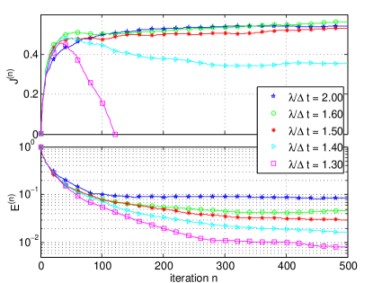
Figure 1: Convergence behavior of error $\mathfrak{E}^{(n)}=1-\mathfrak{F}^{(n)}$ of actual objective, and regularized objective $\mathfrak{J}^{(n)}$ for problem 1 detailed in the appendix with finite time step $\Delta=0.01$ for different values of $\lambda$ shows that monotonic increase of the regularized objective is not guaranteed in the discrete case if the weight of the penalty $\lambda$ is too small. (Initial field ${\bf f}^{(0)}\equiv 0$, $\eta=1$, $\eta^{\prime}=0$, i.e., standard PK-Krotov-update, average cost per forward/backward sweep/iteration $\approx 10.4$ seconds.)

For the typical choices of the objective functional $\mathfrak{F}$ listed above, this scheme can be shown to yield a monotonic increase of the regularized objective function

$$\mathfrak{J}({\bf f})=\mathfrak{F}({\bf f})-\mathfrak{C}({\bf f}),\quad\mathfrak{C}({\bf f})=\textstyle\tfrac{1}{2}\sum_{m}\|f_{m}\|_{w}^{2},$$ (11a)

$$\|f_{m}\|_{w}^{2}=\int_{0}^{T}\!\!|f_{m}(t)|^{2}w_{m}(t)\,dt$$ (11b)

between sweeps (and in fact throughout progression of the pointer $p$) for any positive functions $w_{m}(t)$ and any choice of $\eta,\eta^{\prime}\in[0,2]$ maday_new_2003 . As $\mathfrak{F}({\bf f})$ is uniformly bounded, the sequence $\mathfrak{J}^{(n)}$ is bounded and must converge to some value $\mathfrak{J}_{*}$. However, the best we can hope for is convergence to a critical point of $\mathfrak{J}({\bf f})$, i.e., a point for which the variation of $\mathfrak{J}({\bf f})$ with regard to independent variations of the fields $f_{m}(t)$,

$$\frac{\delta\mathfrak{J}({\bf f})}{\delta f_{m}(t)}=\frac{\delta\mathfrak{F}({\bf f})}{\delta f_{m}(t)}-f_{m}(t)w_{m}(t)$$ (12)

vanishes, which happens if $f_{m}(t)=\frac{1}{w_{m}(t)}\frac{\delta\mathfrak{F}({\bf f})}{\delta f_{m}(t)}$. On the other hand, a necessary condition for the functional $\mathfrak{F}({\bf f})$ to have an extremum is

$$\frac{\delta\mathfrak{F}({\bf f})}{\delta f_{m}(t)}=0\quad\forall m.$$ (13)

This shows that this update scheme generally will not converge to a critical point, much less extremum, of the actual objective $\mathfrak{F}({\bf f})$, as the only critical point shared by the actual objective $\mathfrak{F}$ and the regularized objective $\mathfrak{J}$ is the trivial solution ${\bf f}=0$. In fact, convergence in the stronger sense of convergence of the field iterates ${\bf f}^{(n)}$ to some field ${\bf f}_{\ast}$ that satisfies the critical point condition (12) does not follow trivially, and has only been shown under certain conditions such as sufficiently large penalty terms salomon_limit_2005 , for which the resulting converged fields tend to be far from the global optimum of the unpenalized objective function, as can be seen by comparing the respectively critical point conditions (12) and (13).

Furthermore, numerical solution of the initial and final value problems generally requires some form of time discretization. For a fixed time step $\Delta t$ the change of the regularized objective $\mathfrak{J}$ depends on the choice of the weights $w_{m}$ of the penalty terms and monotonic increase is not guaranteed. When the weights are too small relative to the time step $\Delta t$, the changes in the field amplitudes can become too large and as a result $\mathfrak{J}$ may decrease. An example of this behavior is shown in Fig. 1 for a model system consisting of a linear arrangement of five qubits with uniform, nearest neighbor Heisenberg coupling subject to a fixed global magnetic field in the $x$-direction and five local $Z$-controls, one for each qubit, leading to a Hamiltonian of the form

$$\begin{split}H=&J\sum_{n=1}^{4}\hat{\sigma}_{x}^{(n)}\hat{\sigma}_{x}^{(n+1)}+\hat{\sigma}_{y}^{(n)}\hat{\sigma}_{y}^{(n+1)}+\hat{\sigma}_{z}^{(n)}\hat{\sigma}_{z}^{(n+1)}\\ &+\Omega\sum_{n=1}^{N}\hat{\sigma}_{x}^{(n)}+\sum_{n=1}^{5}f_{n}(t)\hat{\sigma}_{z}^{(n)},\end{split}$$ (14)

where $\hat{\sigma}_{x}^{(n)}$ etc are the usual tensor products of Pauli matrices, e.g., $\hat{\sigma}_{x}^{(1)}=\hat{\sigma}_{x}\otimes I\otimes I\otimes I\otimes I$ and $\hat{\sigma}_{x}$, $\hat{\sigma}_{y}$ and $\hat{\sigma}_{z}$ the the standard Pauli matrices and $I$ the $2\times 2$ identity matrix. For the following simulations we choose the constants $\Omega=10$ and $J=1$.

The convergence plot shows the value of the actual objective $\mathfrak{F}^{(n)}=\frac{1}{32}\Re\operatorname{Tr}(V^{\dagger}U^{(n)}(T))$, the unit gate fidelity, and the regularized objective $\mathfrak{J}^{(n)}=\mathfrak{F}^{(n)}-\mathfrak{C}^{(n)}$ with the penalty term $\mathfrak{C}^{(n)}=\frac{1}{2}\sum_{m}\|f_{m}^{(n)}\|_{w}^{2}$ with uniform weights $w_{m}(t)=\lambda$, as a function of the iteration number $n$ for $\Delta t=0.01$ and different values of $\lambda$. For the smaller values of $\lambda$, $\mathfrak{J}^{(n)}$, after increasing monotonically for a few dozen iterations, starts to decrease as the cost term begins to dominate. One would usually terminate the algorithm at this point but forcing it to continue shows that despite the decrease in $\mathfrak{J}^{(n)}$, the value of the actual objective functional $\mathfrak{F}^{(n)}$ continues to increase. Monotonicity of $\mathfrak{J}^{(n)}$ can be recovered by increasing the weight of the penalty but at the expense of very low final fidelities, which casts doubt on whether optimizing a regularized objective is sensible at all if the real objective is to maximize the fidelity. This problem has also been observed in the literature and as a remedy, a modified version of the regularized objective function $\mathfrak{J}^{\prime}({\bf f})=\mathfrak{F}({\bf f})-\mathfrak{C}_{2}({\bf f})$ with a cost term

$$\mathfrak{C}_{2}({\bf f})=\frac{1}{2}\sum_{m}\|f_{m}-a_{m}\|_{w}^{2}$$ (15)

has been employed reich_monotonically_2010 . It can be shown that if the “reference functions” $a_{m}(t)$ are chosen to be the values of the fields $f_{m}(t)$ in the previous iteration in the iterative update scheme above, giving rise to a dynamic cost term

$$\mathfrak{C}_{2}^{(n)}({\bf f})=\frac{1}{2}\sum_{m}\|f_{m}^{(n)}-f_{m}^{(n-1)}\|_{w}^{2},$$ (16)

then we obtain the modified update rules for the forward and backward sweep

$$\lim_{t\to p^{+}}f_{m}(t)+\frac{\eta}{w_{m}(p)}\frac{\delta\mathfrak{F}({\bf f})}{\delta f_{m}(p)}$$ (17a)

$$\lim_{t\to p^{-}}f_{m}(t)+\frac{\eta^{\prime}}{w_{m}(p)}\frac{\delta\mathfrak{F}({\bf f})}{\delta f_{m}(p)},$$ (17b)

which lead to a monotonic increase in the actual objective $\mathfrak{F}$ for $\eta,\eta^{\prime}>0$. If the sequence of field iterates ${\bf f}^{(n)}$ converges to some field ${\bf f}_{*}$ then we further have $\|f_{m}^{(n)}-f_{m}^{(n-1)}\|\to 0$, i.e., the cost term vanishes in the limit, $\lim_{n\to\infty}\mathfrak{C}_{2}^{(n)}=0$, thus the resulting field ${\bf f}_{*}$ approaches a critical point of actual objective $\mathfrak{F}({\bf f})$. However, such convergence is not guaranteed.

III Optimization of Objective without Penalty

The previous section shows that optimizing a regularized objective with a fixed cost term is problematic in that (i) the critical points of the regularized objective differ from those of the actual objective and (ii) in the discrete time setting even monotonicity cannot be guaranteed. The former issue can be addressed by introducing a variable penalty term but at the expense of compounding technical problems about monotonicity and convergence. We shall now show that the introduction of a regularized objective is unnecessary, and in fact undesirable in particular in the discrete time setting.

As observed above, a necessary condition for the fidelity $\mathfrak{F}({\bf f})$ (infidelity or error $\mathfrak{E}({\bf f})$) to assume a maximum (minimum) at some ${\bf f}={\bf f}_{*}$ is that ${\bf f}_{*}$ be a critical point of $\mathfrak{F}({\bf f})$, i.e., that the variation of $\mathfrak{F}({\bf f})$ with respect to ${\bf f}$ vanish for ${\bf f}={\bf f}_{*}$. As all the objective functionals defined above are simple functionals of the evolution operator $U_{{\bf f}}(t)$, their respective critical points are defined in terms the critical points of $U_{{\bf f}}(t)$, which can be found by rewriting the Schrodinger equation in integral form

$$U_{{\bf f}+\Delta{\bf f}}(t)-U_{{\bf f}}(t)=-i\int_{t_{0}}^{t}U_{{\bf f}}(t,\tau)\Delta H(\tau)U_{{\bf f}+\Delta{\bf f}}(\tau)d\tau$$ (18)

as can be verified simply by differentiating both sides, with $\Delta H(\tau)=H_{{\bf f}+\Delta{\bf f}}(\tau)-H_{{\bf f}}(\tau)$ and $U(t_{2},t_{1})=U(t_{2})U(t_{1})^{\dagger}$. Iteratively substituting (18) into itself yields a perturbative series expansion similar to a Taylor expansion for ordinary functions

$$U_{{\bf f}+\Delta{\bf f}}(t)=U_{{\bf f}}(t)-i\int_{0}^{t}U_{{\bf f}}(t,\tau)\Delta H(\tau)U_{{\bf f}}(\tau)d\tau\\ -\!\!\!\underset{0<\tau_{1}<\tau_{2}<t}{\int\!\!\!\int}\!\!\!\!\!\!U_{{\bf f}}(t,\tau_{2})\Delta H(\tau_{2})U_{{\bf f}}(\tau_{2},\tau_{1})\Delta H(\tau_{1})U_{{\bf f}}(\tau_{1})d\tau_{1}d\tau_{2}\\ +\text{higher order terms}.$$ (19)

The $(n+1)$th term in the expansion (19)

$$(-i)^{n}\underset{0<\tau_{1}<\cdots<\tau_{n}<t}{\int\cdots\int}U_{{\bf f}}(t,\tau_{n})\Delta H(\tau_{n})U_{{\bf f}}(\tau_{n})\\ \cdots U_{{\bf f}}(\tau_{1})^{{\dagger}}\Delta H(\tau_{1})U_{{\bf f}}(\tau_{1})d\tau_{1}\cdots d\tau_{n}$$ (20)

can be bounded by $\tfrac{1}{n!}\|\Delta H\|_{1}^{n}$, where $\|\Delta H\|_{1}$ refers to $\int_{0}^{t}\|\Delta H(\tau)\|d\tau$ for any chosen unitarily invariant norm. This shows that the maps ${\bf f}\mapsto U_{{\bf f}}(t)$ have functional derivatives of all orders for all $t$ and are in a well-defined sense real analytic. By the polarization method, these expansions determine all mixed (functional) derivatives of both $U_{{\bf f}}(T)$ and $U_{{\bf f}}$, with the $n^{th}$ order derivative in directions ${\bf f}_{1},\ldots,{\bf f}_{n}$ bounded in norm by $C^{n}\prod_{k=1}^{n}\|{\bf f}_{k}\|_{1}$ in both cases.

Assuming ${\bf f}=(f_{1}(t),\ldots,f_{M}(t))$ is a vector of independent controls $f_{m}(t)$ in a suitable function space such as $L^{q}[0,T]$ for $q>1$, for example, defining the local variations of the Hamiltonian with respect to the controls $H_{m}(p)=\tfrac{\delta H_{{\bf f}}(p)}{\delta f_{m}(p)}$, we see that the variation of the evolution operator with respect to local variations of the controls are given by

$$\frac{\delta U_{{\bf f}}(t)}{\delta f_{m}(p)}=-iU_{{\bf f}}(t,p)H_{m}(p)U_{{\bf f}}(p),$$ (21)

from which we can effectively compute the variations of all of the objective functionals defined in the previous section, giving for instance,

$$\tfrac{\delta\mathfrak{F}_{3}({\bf f})}{\delta f_{m}(p)} =\textstyle\int_{p}^{T}\!\!\Im\langle\Phi_{d}(t)|U_{{\bf f}}(t,p)H_{m}(p)|\Psi_{{\bf f}}(p)\rangle\,dt$$

$$\tfrac{\delta\mathfrak{F}_{4}({\bf f})}{\delta f_{m}(p)} =\textstyle\int_{p}^{T}\!\!\operatorname{Tr}(Q(t)U_{{\bf f}}(t,p)[\rho_{{\bf f}}(p),iH_{m}(p)]U_{{\bf f}}(p,t))\,dt$$

$$\tfrac{\delta\mathfrak{F}_{6}({\bf f})}{\delta f_{m}(p)} =\textstyle\int_{p}^{T}\!\!2\Im\langle\Psi_{{\bf f}}(t)|Q(t)U_{{\bf f}}(t,p)H_{m}(p)|\Psi_{{\bf f}}(p)\rangle\,dt.$$

Given any $\mathfrak{F}$ that is a sum of multi-linear terms in $U_{{\bf f}}(T)$ and $U_{{\bf f}}$ that are bounded in all entries of $U_{{\bf f}}$, we can easily devise schemes that lead to a monotonic increase of $\mathfrak{F}$. Let $b$ be a positive function that vanishes outside the interval $[-1,1]$ and integrates to $1$, and let $b_{s,p}(x)=b((x-p)/s)$ be the rescaled version of $b$ centered at point $p$. Assuming ${\bf f}(p)$ bounded about $p$ and $s\leq p,T-p$, the gradient of $U_{{\bf f}}(T)$ with respect to $b_{s}$ is

$$-i\int_{p-s}^{p+s}U_{{\bf f}}(T,\tau)b_{s,p}(\tau)H_{m}(p)U_{{\bf f}}(\tau)\,d\tau\\ =-isU_{{\bf f}}(T,p)H_{m}(p)U_{{\bf f}}(p)+O(s^{2})$$ (23)

since $U_{{\bf f}}(\tau)$ is locally Lipschitz at $\tau=p$, where the error term is bounded independently of $b$. Under the same assumptions, the gradient of $U_{{\bf f}}(t)$ in direction $b_{s}$ is the function of $t$

$$\left\{\begin{array}[]{r@{\qquad}l}-isU_{{\bf f}}(t,p)H_{m}(p)U_{{\bf f}}(p)&t>p\\ 0&\text{otherwise}\end{array}\right.$$ (24)

up to an $O(s^{2})$ error, as measured in any $L^{q}$ norm with $q<\infty$. Applying the product rule to our general $\mathfrak{F}$ with the approximations (23) and (24), dividing by $s$, then letting $s\rightarrow 0$, shows that the value $\frac{\delta\mathfrak{F}({\bf f})}{\delta f_{m}(p)}$ is always well-defined and yields an expression for it. The exact sense in which this quantity matches the derivative of $\mathfrak{F}$ evaluated at a $\delta$-mass is that $b$ is a positive mollifier. Denoting the addition of $\alpha b_{s}$ to the $m$th field $f_{m}$ by ${\bf f}+\alpha b_{s}\mathbb{I}_{m}$, a Taylor expansion to first order gives

$$\mathfrak{F}({\bf f}+\alpha b_{s}\mathbb{I}_{m})=\mathfrak{F}({\bf f})+\alpha s\frac{\delta\mathfrak{F}({\bf f})}{\delta f_{m}(p)}+O(s^{2})$$ (25)

for each $\alpha$. This shows that for any $\alpha$ of the same sign as $\frac{\delta\mathfrak{F}({\bf f})}{\delta f_{m}(p)}$, assuming the former is non-zero, there is a sufficiently small scale $s$ for which adding $\alpha b_{s}$ to the field leads to an increase in $\mathfrak{F}$. Thus, if we add a sequence of such increments $\alpha b_{s,p_{k}}$ centered at different times $p_{k}$, the corresponding sequence $\mathfrak{F}^{(k)}$ will be monotonically increasing. For a fidelity function $\mathfrak{F}$, which is a continuous function from the compact domain $\mathbf{U}(N)$ to $\mathbb{R}$, the range of $\mathfrak{F}$ is bounded. Thus $\mathfrak{F}^{(k)}$ is a uniformly bounded, monotonically increasing sequence, i.e., convergent. Convergence of $\mathfrak{F}^{(k)}$ to some value $\mathfrak{F}_{*}$ is not a very strong property, however; what is more interesting is whether we converge to a global maximum of the fidelity, or equivalently, whether the infidelity/error $\mathfrak{E}$ goes to $0$, and the rate of convergence.

Using this update rule, making bigger changes to each $f_{m}$ in its gradient direction should in principle offer larger increases in the fidelity $\mathfrak{F}({\bf f})$ for the same displacement incurred by the pointer $p$. On the other hand, we can expect larger choices of $\alpha$ to directly lead to higher amplitudes of ${\bf f}$, which in turn induce more oscillation in $U_{\bf f}$, the gradients $\frac{\delta\mathfrak{F}({\bf f})}{\delta f_{m}(p)}$ and therefore in the fields. So it would seem that in choosing $\alpha$, we are making a trade-off between high amplitude and oscillation in the fields, which are generally undesirable features, and fast convergence of the algorithm. To make this intuition about speed rigorous, we can prove that there is an upper bound on the instantaneous rate of convergence which increases with the search length $\alpha$ and tends to zero as $\alpha$ vanishes. However, this is a static analysis that cannot take into account the evolution of the algorithm. Once we move to a more sophisticated ‘stateful’ analysis, we can derive a different bound on the asymptotic rate of convergence which is actually decreasing in the search length $\alpha$. The resulting bounds on the asymptotic convergence rates in the continuous limit are shown in Fig. 2. The non-trivial stateful bound in particular shows that larger search lengths, which are bound to result in greater speeds towards the start of the algorithm, will tend to slow down optimization in the long run, at least past a certain value of $\alpha$.

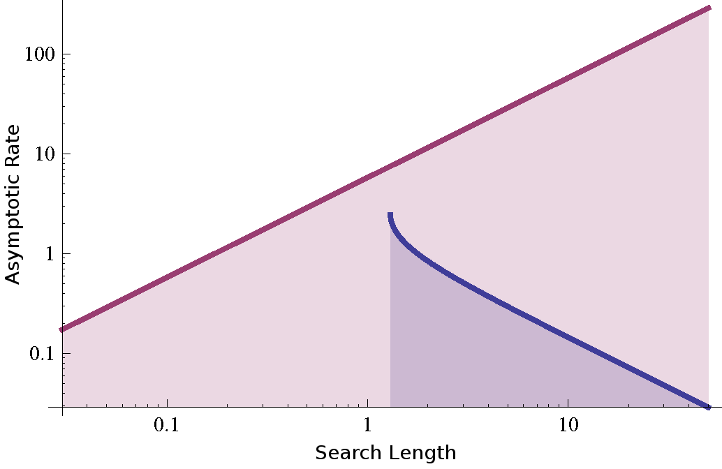
Figure 2: Static (red, increasing) and stateful (blue, decreasing) upper bounds on the asymptotic rate of convergence for back-and-forth sweeping in the continuous limit $s\to 0$ for a single control field show that there is an asymptotic rate that cannot be exceeded no matter what search length $\alpha$ is used.

IV Field discretization and practical optimization schemes

The previous section shows that we can in principle easily monotonically increase the objective function by iteratively updating the controls in a sequence of forward and backward sweeps. In practice solving the optimal control problem numerically requires discretization of time. This is often done implicitly but we shall see that the choice of discretization restricts the class of monotonic schemes that are available compared to the continuous case. It is therefore desirable to explicitly discretize the problem and derive optimization schemes for this case. We can do this by choosing a basis function $b$, with a step size $s$ and a set of positions $p_{k}$. The most common choice is to partition of the interval $[0,T]$ into a fixed number of intervals of size $\Delta t=T/K$ and restrict the controls $f_{m}(t)$ to be piecewise constant functions

$$f_{m}(t)=\sum_{k=1}^{K}f_{mk}\chi_{k},$$ (26)

where $\chi_{k}$ is the characteristic function of the interval $I_{k}=[t_{k-1},t_{k})$, $t_{0}=0$ and $t_{K}=T$. In this case we have

$$\mathfrak{F}({\bf f}+\alpha\chi_{k}\mathbb{I}_{m})=\mathfrak{F}({\bf f})+\alpha\frac{\partial\mathfrak{F}({\bf f})}{\partial f_{mk}}+O(\alpha^{2}\Delta t^{2}),$$ (27)

where $\mathbb{I}_{m}$ indicates that we are adding the basis function to the field $f_{m}(t)$. For a given fixed $\Delta t$ the $O(\alpha^{2}\Delta t^{2})$ term in Eq. (27) need not be negligible and $\alpha$ must be chosen carefully to ensure $\mathfrak{F}({\bf f}+\alpha\chi_{k}\mathbb{I}_{m})\geq\mathfrak{F}({\bf f})$. In theory choosing the time step $\Delta t$ and search length $\alpha$ small will ensure $\mathfrak{F}({\bf f}+\alpha\chi_{k}\mathbb{I}_{m})\geq\mathfrak{F}({\bf f})$, i.e., a monotonic increase in the objective functional, but this will result in tiny increases in the objective function in each step and thus slow convergence. For the discretized version of the problem one can actually prove stronger convergence results in the sense that under relatively mild conditions, the sequence of field iterates ${\bf f}^{(n)}$ must either converge to a critical point ${\bf f}_{\ast}$ of the fidelity function or diverge to infinity (see appendix B).

IV.1 Time Resolution and Gradient Accuracy

The first critical choice we have to make is the time resolution or time step $\Delta t$, which effectively determines the finite-dimensional subspace of the infinite-dimensional function space $L^{q}[0,T]$ we choose to restrict the optimization to. Considering that we started with a continuous-time optimal control problem, it may seem natural to choose small time steps $\Delta t$ to approximate the continuous case, and it is certainly true that choosing $\Delta t$ too large may prevent us from being able to reach high fidelities by restricting the search space too much. In general, a minimum requirement for controllability is that the dimensionality of the search space $M\times K$ be no less than the dimension of the state space. For optimization of five-qubit unitary gates, for example, the state space is the unitary group $\mathbf{U}(32)$, which has dimension $32^{2}$. Thus we will require at least $MK\geq 1024$ and higher time resolutions may be necessary to achieve high fidelities, although the fidelities considered satisfactory in practice may be low in this context. But aside from such considerations, small time steps are not necessarily a good idea. Simple analysis shows that the computational cost per iteration for a fixed problem and system size $N$ is determined by the number of time steps $K$, and thus $\Delta t=T/K$ if the target time $T$ is fixed. Higher time resolutions, i.e., smaller $\Delta t$, are therefore computationally more expensive. Of course, this cost may be offset by larger gains per iteration. However, we shall see that the discrete rate of convergence is always of order $\Delta t$, and for unitary gate optimization problems with fixed proportional search length the upper bound on the rate of convergence is of order $\Delta t^{2}$, for example, suggesting that larger $\Delta t$ may actually facilitate faster convergence. Another reason why very small time steps are often undesirable are the characteristics of the fields, e.g., to avoid excessively complex and noisy solutions.

Choosing larger $\Delta t$ requires careful reconsideration of the gradient computation, however. Assuming for simplicity that the total Hamiltonian is linear in the controls

$$H[{\bf f}]=H_{0}+\sum_{m=1}^{M}f_{m}H_{m},$$ (28)

with time-independent $H_{m}$, we have $\delta H[{\bf f}]/\delta f_{m}=H_{m}$ and Eq. (19) gives immediately

$$\frac{\partial U_{{\bf f}}(T)}{\partial f_{mk}}=U_{{\bf f}}(T,t_{k})J_{mk}U_{{\bf f}}(t_{k},t_{0})$$ (29a)

$$J_{mk}=\int_{t_{k-1}}^{t_{k}}\!\!\!U_{{\bf f}}(t_{k},t)(-iH_{m})U_{{\bf f}}(t,t_{k})\,dt,$$ (29b)

from which we can calculate the various gradients, after setting $\langle\Phi_{{\bf f}}(t_{k})|:=\langle\Phi|U_{{\bf f}}(T,t_{k})$ and $Q_{{\bf f}}(t_{k}):=U_{{\bf f}}(T,t_{k})^{\dagger}QU_{{\bf f}}(T,t_{k})$, as

$$\tfrac{\partial\mathfrak{F}_{1}}{\partial{\bf f}_{mk}} =\Re\langle\Phi_{\bf f}(t_{k})|J_{mk}|\Psi_{\bf f}(t_{k})\rangle$$

$$\tfrac{\partial\mathfrak{F}_{1b}}{\partial{\bf f}_{mk}} =2\Re(\langle\Phi_{\bf f}(t_{k})|J_{mk}|\Psi_{\bf f}(t_{k})\rangle\langle\Psi_{\bf f}(t_{k})|\Phi_{\bf f}(t_{k})\rangle)$$

$$\tfrac{\partial\mathfrak{F}_{2}}{\partial{\bf f}_{mk}} =\operatorname{Tr}(Q_{\bf f}(t_{k})[J_{mk},\rho_{\bf f}(t_{k})])$$

$$\tfrac{\partial\mathfrak{F}_{5}}{\partial{\bf f}_{mk}} =2\Re\langle\Psi_{\bf f}(T)|QU_{\bf f}(T,t_{k})J_{mk}|\Psi_{\bf f}(t_{k})\rangle$$

$$\tfrac{\partial\mathfrak{F}_{7}}{\partial{\bf f}_{mk}} =\Re\operatorname{Tr}(V^{{\dagger}}U_{\bf f}(T,t_{k})J_{mk}U_{\bf f}(t_{k}))$$

$$\tfrac{\partial\mathfrak{F}_{7b}}{\partial{\bf f}_{mk}} =\Re\left(\operatorname{Tr}(V^{{\dagger}}U_{\bf f}(T,t_{k})J_{mk}U_{\bf f}(t_{k}))\tfrac{\overline{\operatorname{Tr}(V^{{\dagger}}U_{\bf f}(T))}}{|\operatorname{Tr}(V^{{\dagger}}U_{\bf f}(T))|}\right).$$

For small $\Delta t$ the integral defining $J_{mk}$ can be approximated by replacing the integrand by its value at some point, e.g., the right endpoint

$$J_{mk}\approx(-iH_{m})\Delta t.$$ (31)

The accuracy of this first-order approximation depends on $\Delta t$ and the eigenvalues of the total Hamiltonian $H({\bf f})=H_{0}+\sum_{m}f_{m}(t)H_{m}$, i.e., the approximation is liable to break down when norm of any of the Hamiltonians $H_{m}$ is large, or if the field amplitudes become too large unless very small time steps are used. For piecewise constant controls $H[{\bf f}(t_{k})]$ is constant on the interval $I_{k}$, and it is easy to derive an exact formula for the gradient by evaluating the integrals $J_{mk}$ analytically, noting that $U_{{\bf f}}(t_{k},t)=e^{(t_{k}-t)B}$, and thus

$$\begin{split}J_{mk}&=\int_{0}^{\Delta t}e^{\tau B}(-iH_{m})e^{-\tau B}d\tau\\ &=\gamma(\Delta t\operatorname{ad}_{B})(-iH_{m})\Delta t\end{split}$$ (32)

where $B=-iH({\bf f}(t_{k}))$ and

$$\gamma(z)=\frac{e^{z}-1}{z}=\sum_{n=0}^{\infty}\frac{z^{n}}{(n+1)!}.$$ (33)

For Hamiltonian systems $\gamma(z)$ can be evaluated via the eigendecomposition of the skew-Hermitian matrix $B=V\Lambda V^{\dagger}$, where $\Lambda=\operatorname{diag}(\lambda_{r})$ and $\lambda_{r}$ purely imaginary. This allows us to evaluate $\gamma(\Delta t\operatorname{ad}_{B})(-iH_{m})$, noting that

$$J_{mk}=\sum_{r,s=1}^{N}|v_{r}\rangle\langle v_{r}|J_{mk}|v_{s}\rangle\langle v_{s}|$$ (34)

where $\langle v_{r}|J_{mk}|v_{s}\rangle$ are determined by $\gamma(z)$ evaluated at the eigenvalues of the adjoint $\operatorname{ad}_{B}$ times $\Delta t$, which are determined by the differences of eigenvalues $\lambda_{r}$ of $B$, $\omega_{rs}=\lambda_{r}-\lambda_{s}$:

$$\langle v_{r}|J_{mk}|v_{s}\rangle=\gamma(\omega_{rs}\Delta t)\langle v_{r}|-iH_{m}|v_{s}\rangle\Delta t.$$ (35)

The first order approximation $\gamma(\omega_{rs}\Delta t)=1$ is off by close to $\min\{\Delta t|\omega_{rs}|/2,1\}$. Thus, to ensure that the standard approximation is reasonably accurate we require $\Delta t<\|\operatorname{ad}_{B}\|^{-1}$ where $\|A\|$ is the operator norm, $\max|{\rm eig}(A)|$. In problem 1 it can be shown that $\|\operatorname{ad}_{B}\|\approx 100$, with the dominant contribution being $H_{0}$, which shows that for $\Delta t=0.01$ standard approximation is over 95% accurate while for $\Delta t=0.1$, $x$ can be as large as $10$, i.e., $\gamma(ix)$ is far from $1$ and the error in the gradients is huge, and we are in fact performing more of a random walk than a gradient search! A histogram of the actual distribution of the gradient overlaps

$$\frac{\langle\nabla\mathfrak{F}_{\rm exact}|\nabla\mathfrak{F}_{\rm approx}\rangle}{\|\nabla\mathfrak{F}_{\rm exact}\|\cdot\|\nabla\mathfrak{F}_{\rm approx}\|}$$ (36)

for problem 1 in Fig. 4 confirms this, showing that the first order approximation is excellent for $\Delta t=0.01$ — the distribution is narrow with a median overlap of 99.77% — while for $\Delta t=0.1$ the distribution is broad with a median overlap of only $41.80$%.

Figure 3: $\gamma(ix)$ shows that $|\gamma(ix)|$ is close to $1$ for $|x|<1$ but quickly drops off for larger $x$ leading to large errors in the standard gradient approximation.

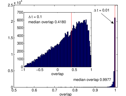
Figure 4: Histogram plot of overlap of first order gradient approximation with the exact gradient for problem 1 for $\Delta t=0.01$ and $\Delta t=0.1$ (red lines: medians).

Alternatively, it can be verified by induction that

$$(\Delta t\operatorname{ad}_{B})^{n}H_{m}=\sum_{k=0}^{n}\left(\begin{array}[]{c}n\\ k\end{array}\right)\Delta t^{n}B^{n-k}H_{m}(-B)^{k}$$ (37)

leading to

$$\gamma(\Delta t\operatorname{ad}_{B})H_{m}=\sum_{n=0}^{\infty}\frac{\Delta t^{n}}{n+1}\sum_{k=0}^{n}\frac{B^{n-k}H_{m}(-B)^{k}}{(n-k)!k!}.$$ (38)

One possibility to evaluate this series is to truncate the infinite sum at some $N-1\geq 1$ and invert the order of summation to reduce the number of required matrix products to $3N-4$. Any such sum of the first $N$ terms of the series yields an approximation to the exact gradient expression of order $N$ in $\Delta t$. For $N$ even we can reduce the number of required products to $2N-2$ by summing $N/2$ terms of the form

$$a_{j}\left(\sum_{k=0}^{N-1}r_{j}^{k}\frac{\Delta t^{k}B^{k}}{k!}\right)H_{m}\left(\sum_{k=0}^{N-1}(-r_{j})^{k}\frac{\Delta t^{k}B^{k}}{k!}\right)$$ (39)

for suitable choices of $a_{j},r_{j}$. To recover the first $N$ terms in the series, the coefficients $a_{j},r_{j}$ must satisfy

$$\sum_{j=1}^{N/2}a_{j}r_{j}^{n}=\frac{1}{n+1}=\int_{0}^{1}x^{n}\,dx$$ (40)

for $n=0,\ldots,N-1$. This relation uniquely determines the $r_{j}$ as the nodes, and $a_{j}$ as the corresponding weights of Gauss-Legendre quadrature over the interval $[0,1]$.

The series expansion is preferable to the eigendecomposition for pure-state or state vector optimization problems; in particular for a fidelity function such as $\mathfrak{F}_{1}$, $\mathfrak{F}_{1b}$ or $\mathfrak{F}_{5}$, whose gradient in step $k$ is expressible in terms of the real inner product of the state $|\Psi_{{\bf f}}(t_{k})\rangle$ and some vector $\langle\Phi|$, as $\langle\Phi|J_{mk}|\Psi_{{\bf f}}(t_{k})\rangle$. This expression can be approximated to order $N$ by first computing $B^{k}|\Psi_{{\bf f}}(t_{k-1})\rangle$ and $\langle\Phi_{{\bf f}}(t_{k-1})|B^{k}$ for $k=1,\ldots,N-1$ and then applying either of (38) or (39). These procedures use only matrix-vector or vector-vector operations, avoiding the need for relatively expensive matrix multiplications and an eigendecomposition. Specifically, Eq. (38) needs $MN+2N-2$ matrix-vector products and $N((N+1)/2+M)$ vector operations to evaluate for all controls, while Eq. (39) achieves the same order of approximation with only $MN/2+2N-2$ and $(N+M)N/2$ operations respectively. The series expansion therefore can be applied to state transfer problems for high-dimensional systems with sparse Hamiltonians, where the eigendecomposition is infeasible. However, additional measures such as scaling and squaring may be needed for larger time steps to ensure that the series approximation can be truncated for small $N$. Another alternative are finite difference approximations to estimate the gradients. These issues are further explored in the context of spin dynamics for large-scale systems in de_fouquieres_second_2011 .

We can also derive an efficient series approximation for density matrix and unitary gate optimization problems with fidelity functions $\mathfrak{F}_{2}$, $\mathfrak{F}_{7}$ or $\mathfrak{F}_{7b}$. The gradients on step $k$ of these fidelities can all be expressed as $\operatorname{Tr}(AJ_{mk})$ for some skew-Hermitian matrix $A$, which is $[\rho_{\bf f}(t_{k}),Q_{\bf f}(t_{k})]$ for $\mathfrak{F}_{2}$, and the skew-Hermitian part $(X-X^{\dagger})/2$ of $X=U_{\bf f}(t_{k})V^{\dagger}U_{\bf f}(T,t_{k})$ for $\mathfrak{F}_{7}$ or the phase multiple of $X$ for $\mathfrak{F}_{7b}$. Using the fact $\operatorname{Tr}(W[X,Y])=\operatorname{Tr}([W,X]Y)$ iteratively, we can re-write $\operatorname{Tr}(AJ_{mk})$ as

$$-\operatorname{Tr}\left(\sum_{n=0}^{\infty}\frac{\Delta t^{n}}{(n+1)!}\operatorname{ad}_{-B}^{n}(A)iH_{m}\right)\Delta t,$$ (41)

which when truncated to its first $N$ terms, requires $N-1$ matrix multiplications (plus $N+M$ negligible element-wise matrix operations) to evaluate for all controls, noting that the commutator $[X,Y]$ of skew-Hermitian matrices $X,Y$ is the skew-Hermitian part of $2XY$. Formula (35), however, has the advantage of being exact, and its numerical cost being independent of $\Delta t$. Furthermore, once the eigendecomposition of $H[{\bf f}(t_{k})]$ is known, the computation of the evolution operators $U_{{\bf f}}(t_{k},t_{k-1})$ becomes trivial. This makes it suitable — and in many cases probably preferable — for use in density matrix and unitary gate optimization problems.

IV.2 Variants of Sequential Update

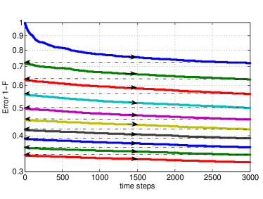
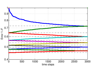
Figure 5: Evolution of fidelity (first 10 iterations) for forward-only (top) forward-backward (middle) and split (bottom) update for $\Delta t=0.01$. For continuous forward-backward sweeps the gradient quickly becomes very small and the fidelity barely increases after a few iterations. For the forward-only and split update the switch-overs enable revival of the gradients and thus the rate of fidelity decrease, thereby accelerating convergence.

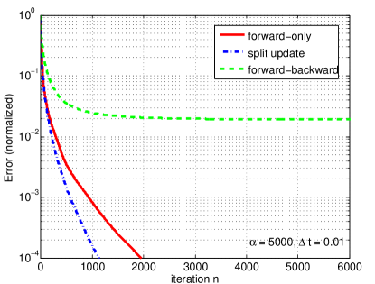
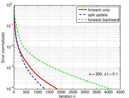
Figure 6: Convergence behavior for forward-only, forward-backward and split update for $\Delta t=0.01$ and $\alpha=5000$ and $\Delta t=0.1$ and $\alpha=200$ shows that forward-only update is preferable to back-and-forth update and split update is even better. The differences decrease with larger time steps.

The straightforward discrete analogue of the continuous forward and/or backward sweeping is sequentially updating the fields ${\bf f}(t_{k})$ for $k=1$ to $k=K$ (or $k=K$ to $k=1$) according to the rule

$${\bf f}^{(n+1)}(t_{k})={\bf f}^{(n)}(t_{k})+\alpha\nabla_{k}\mathfrak{F}({\bf f}^{(n)}),$$ (42)

where $\nabla_{k}\mathfrak{F}=(\tfrac{\partial\mathfrak{F}}{\partial f_{mk}})_{m=1}^{M}$ is the gradient vector at time $t_{k}$, and iterating the procedure, starting with an initial trial field ${\bf f}^{(0)}$ as before. As in the continuous case, we have the option of sweeping forward and backward, continually updating the fields in both directions, as e.g., in zhu_rapid_1998 and the generalized scheme proposed by maday_new_2003 , or updating the fields only in one direction, usually the forward sweep, as in the PK-Krotov version of the iterative update scheme discussed in Sec. II, where $\eta=1$ and $\eta^{\prime}=0$. Intuitively one might expect that updating the fields in both directions should accelerate convergence, but convergence analysis shows that this is not the case. Continually updating the fields in both directions in fact reduces the asymptotic rate of convergence.

This is illustrated in Fig. 6, which shows that the asymptotic rate of convergence is substantially greater for the forward-only update than for forward-backward update, in particular for small $\Delta t$, i.e., updating on the forward sweep only is preferable to updating on both sweeps. This can intuitively be explained as follows. The sequential update scheme aims to minimize the gradient at each time step. By continuity, minimizing the gradient at time $t_{k}$ tends to decrease the gradient at the subsequent time step $t_{k+1}$. As the magnitude of the gradient is the main factor limiting the increments in the fidelity at each time step, we quickly reach an asymptotic regime. If we only update in one direction, however, there is a step jump at every iteration, whenever we switch from $t=t_{K}$ to $t=t_{1}$, which allows the gradient to rebound, facilitating larger gains in subsequent steps.

These observations suggest that updating the fields in a strictly sequential manner is not the optimal strategy, and that convergence might be accelerated by introducing step jumps. For example, instead of updating the fields sequentially in a single forward or backward sweep, we could update half the fields ${\bf f}(t_{k})$ in the forward sweep and the other half in the backward sweep. We could choose the fields to be updated in the forward sweep randomly or choose to update all odd time slices $f(t_{2k-1})$ in the forward sweep, and the even ones in the backward sweep. The gains of such schemes per single time slice update must be offset against increased computational overheads associated with such non-sequential updates, chiefly additional matrix multiplications to propagate the changes. However, there is one simple variations of strictly sequential update that can be implemented without increasing the total number of operations (matrix exponentials, matrix multiplications and gradient evaluations) per single iteration: if we update the first $K/2$ time slices consecutively in the forward sweep, propagate without updating to $k=K$, and update the second half of the field consecutively in the backward sweep and then back-propagate from $k=K/2$ to $k=1$ without updating. Fig. 6 shows that this split update strategy outperforms the forward-only update although the gains are smaller than for back-and-forth update versus forward-only update, and the advantage of the split update scheme diminishes for larger time steps, not too surprisingly, as for fewer and larger time steps the local gradients do not die off as fast, and therefore the rebound effect induced by the switch-overs is reduced. The cost per iteration for all update schemes was about $\approx 3.05$ seconds for $\Delta t=0.01$ ($K=3000$) using the first-order gradient approximation, which is accurate for this time step, and $\approx 0.34$ seconds for $\Delta t=0.1$ ($K=300$) using the exact gradient formula . The total operation count (matrix multiplications, propagation steps, gradient evaluations) per iteration for $K=300$ is approximately $1/10$ of the number of operations for $K=3000$. The time per iteration for $K=300$ is slightly greater than one tenth of the time per iteration for $K=3000$, $3.05/10=0.305<0.34$. The additional cost reflects the fact the exact gradient evaluations are slightly more computationally expensive than the first-order approximation.

IV.3 Dynamic Search-length Adjustment

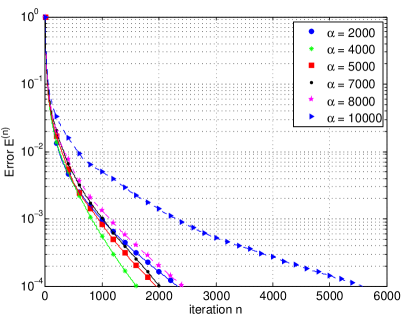
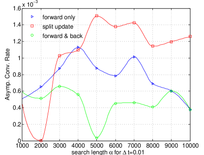
Figure 7: Convergence behavior for sequential optimization without penalty (problem 1, $\Delta t=0.01$, forward-only update) for different choices of the search length parameter $\alpha$ shows significant dependence of convergence rate on $\alpha$ (left). The convergence plots allow estimation of the “asymptotic” convergence rate as a function of $\alpha$, shown right for different update strategies.

Another crucial parameter in the gradient-based sequential optimization is the choice of the search length $\alpha$. Fig. 7 shows that the rate of convergence depends strongly on $\alpha$ even if all other parameters are the same, and we therefore require a way to choose a suitable search length based on a simplified local model of the function to be optimized. As previously explained, a quadratic approximation, say $\tilde{F}(\alpha)$, to the fidelity change

$$F(\alpha)=\mathfrak{F}({\bf f}+\alpha\Delta{\bf f}_{k})-\mathfrak{F}({\bf f})$$ (43)

in some direction $\Delta{\bf f}_{k}$ is often sufficient for the purposes of our optimization problems. Such a second-order model $\tilde{F}$ is determined by matching two quantities in addition to the obvious $\tilde{F}(0)=0=F(0)$, for which it is natural to choose the derivative $\tilde{F}^{\prime}(0)=F^{\prime}(0)$ and value $\tilde{F}(\alpha_{0})=F(\alpha_{0})$ at some $\alpha_{0}$. Assuming that $F^{\prime}(0)=\Delta{\bf f}_{k}^{T}\cdot\nabla_{k}\mathfrak{F}({\bf f})$ is strictly positive, such as with $\Delta{\bf f}_{k}=\nabla_{k}\mathfrak{F}({\bf f})$ the non-zero gradient, all possible $\tilde{F}$ are equivalent up to scale (and a sign), so that we can just consider an appropriately invariant quantity e.g. $\xi=1-\frac{F(\alpha_{0})}{F^{\prime}(0)\alpha_{0}}$. Since $\tilde{F}(\alpha)=F^{\prime}(0)(\alpha-\frac{\xi}{\alpha_{0}}\alpha^{2})$, for $\xi>0$ then $\tilde{F}$ has its second root at $\alpha=\frac{\alpha_{0}}{\xi}$, so its maximum at $\alpha_{\ast}:=\frac{\alpha_{0}}{2\xi}$, while otherwise $\tilde{F}$ is simply unbounded. If the quadratic approximation is accurate, $(2\xi)^{-1}$ is then close to the factor by which we must multiply the current search length $\alpha_{0}$ in order to maximize the fidelity gain $F$ in the current step. Note that this choice of new search length $\alpha_{\ast}$ makes sense even in general, since $\xi$ measures the relative error in the linear expansion $F^{\prime}(0)\alpha$ of $F(\alpha)$ at $\alpha_{0}$ and shrinks or grows $\alpha_{0}$ according to whether and how much this error is above or below one half. We are then aiming for the largest $\alpha$ for which the gradient based model is still relevant, so again the largest reliable fidelity gain, although in the general case, when $\xi^{-1}$ is large or negative, it is safer to let $\alpha_{\ast}$ be some fixed multiple, say $2$, of $\alpha_{0}$. Fig. 8 though, with $F(\alpha)$ and $\tilde{F}(\alpha)$ computed for a randomly chosen time step for problem 1, shows that the quadratic model to be an excellent approximation here, as the theory would lead us to expect.

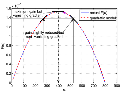
Figure 8: Actual $F(\alpha)$ and quadratic model $\tilde{F}$ for a randomly selected time step $t_{k}$ (problem 1).

These considerations suggest that the locally optimal update strategy is to set the search length $\alpha$ to $\alpha_{*}$ in each step. However, this strategy has one problem: at the local maximum $\alpha_{*}$ the derivative of the second order approximation $\tilde{F}(\alpha)$ vanishes, and thus the derivative of $F(\alpha)$ will be approximately zero as well. By continuity of the gradient this tends to ensure that the gradient at the next time step $t_{k+1}$ will be small, especially for small $\Delta t$. Therefore, the most greedy local update strategy may not be the best in the long run as it rapidly kills off the gradients, thus reducing future gains and decreasing the rate of convergence in the longer run. This effect will be most pronounced for the back-and-forth update, the most greedy update strategy, but it is still significant for forward-only and even split update. This suggests an alternative strategy for choosing $\alpha$. Instead of choosing $\alpha=\alpha_{*}$, we may wish to choose $\alpha$ to be slightly larger or smaller than $\alpha_{*}$. Fig. 8 shows that this will not reduce the local gain very much but has a significant impact on the gradients. Indeed, Fig. 9 shows that the median fidelity averaged over 100 runs using the split-update strategy with the most greedy choice of search length $\alpha=\alpha_{*}$ is slower in the long run than two variants of search length adjustment motivated by the above considerations. Variant 3 in the figure is based on a deliberate overshooting strategy, choosing $\alpha=1.25\alpha_{*}$ in each time step. Variant 1 is aimed at slowly changing the search length until it falls within a desirable range $[r_{1},r_{2}]\alpha_{*}$ around the maximum, and trying to keep it in this range. If the current search length $\alpha<r_{1}\alpha_{*}$ then we increase $\alpha$ by a fixed factor $\alpha_{1}$, if $\alpha>r_{2}\alpha_{*}$ then we decrease $\alpha$ by a factor $\alpha_{2}$. This ensures that whenever $\alpha$ falls outside the desirable range, it is increased or decreased in each step until it falls back in the desirable range. We chose $r_{1}=\frac{2}{3}$ and $r_{2}=\frac{4}{3}$ and $\alpha_{1}=0.99$, $\alpha_{2}=1.01$. The $r$-values are motivated by the quadratic model, while there is no simple rule for choosing $\alpha_{1}$ and $\alpha_{2}$. Our choice of factors very close to $1$ may appear strange and does reduce gains during the first few-hundred time steps if the initial choice of $\alpha$ is far from the optimum value, but even such a small factor allows $\alpha$ to increase 20-fold in a single iteration with $K=300$ steps ($1.01^{300}\approx 20$), and gradual changes can facilitate convergence of $\alpha$ to a near optimal value, especially for gate optimization problems. Fig. 9 suggests that this strategy is clearly better than the most greedy one, though slightly worse than the systematic overshoot strategy when considering only the median fidelity over 100 runs. Systematic overshoot can result in large changes in the search lengths especially initially, leading to instabilities and occasional failure, however. This is evident in Fig. 10, which shows the evolution of the search lengths as a function of the total number of time steps executed for three different search length strategies. In all three cases the search length $\alpha$ quickly approaches a limiting value. The limiting values of $\alpha$ for variant 1 and the systematic overshoot strategy (variant 3) above are very close, and about 30% larger than the limiting value for the most greedy strategy (variant 2). Variant 1, although based on somewhat ad-hoc choices, has the advantage of avoiding fluctuations and large spikes in the search length, especially during the first few hundred time steps when the quadratic model may not be very accurate.

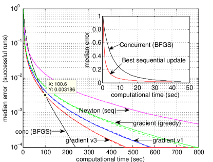
Figure 9: Median fidelity for 100 runs as a function of computational time for different optimization strategies: sequential gradient, sequential Newton and concurrent quasi-Newton update using BFGS algorithm for problem 1 with $\Delta t=0.1$ as a function of the search length $\alpha$.

Another reason why avoidance of large changes from one time step to the next is desirable is computational efficiency. Usually, in optimization problems one would apply any change in the search length immediately, but this is computationally expensive as it requires the computation of a matrix exponential $\exp(-i\Delta tH[{\bf f}(t_{k})])$ for the new field ${\bf f}(t_{k})$, and the gain of increasing the step length for any given time interval is usually small, especially when the search length is close to its optimum. To avoid such overheads one may choose not to apply the search length change at the current step, but only at the next time step. This is not too unreasonable as continuity considerations suggest that the optimal search length should not vary too much from one time step to the next, and it ensures that the computational overhead of the dynamic search length adjustment is negligible and the computational cost per iteration is constant as it would be for a fixed search length. For sequential optimization over many time slices avoiding the computational overhead of multiple fidelity re-evaluations at each time step is usually preferable over the small gain achieved by applying the search length change to the current time interval, and for unitary gate optimization problems in particular, the search length usually quickly approaches an optimal value and varies relatively little after this, as shown in Fig. 10.

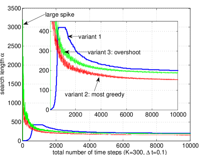
Figure 10: Variation of dynamic search length parameter $\alpha$ as the function of the total number of time steps executed ($K=300$ steps per iteration, $\Delta t=0.1$, forward-only update) for different search length strategies.

IV.4 Higher-Order Methods

In the previous two sections we have considered changing the fields locally in direction $\Delta{\bf f}_{k}$ of the gradient $\nabla_{k}\mathfrak{F}({\bf f})$ using a quadratic model for the fidelity change $F$ along that line as a function of the search length $\alpha$. In general though, there is nothing special about the gradient direction, unless the local Hessian is a scalar multiple of the identity. Thus we should do better if we replace the simple gradient update by a Newton update step:

$$\Delta{\bf f}_{k}=-[\mathfrak{H}^{(k)}]^{-1}\nabla_{k}\mathfrak{F}({\bf f}),$$ (44)

using the full matrix of second order partial derivatives $\mathfrak{H}_{k}$ (Hessian), provided that $\mathfrak{H}^{(k)}$ is strictly negative definite, given that we are maximizing. If the Hessian $\mathfrak{H}^{(k)}$ is indefinite or positive definite, the Newton step should never be used since it would take us to some irrelevant saddle point, or worse the minimum, rather than the desired maximum, of the quadratic model. In these cases, the quadratic model has no unconstrained maximum, and as it is anyway only accurate in a neighborhood of the original ${\bf f}_{k}$, a trust-region method (see Appendix A), which restricts attention to suitably small changes in ${\bf f}_{k}$, should be used.

For sequential update the Hessian matrix for the $k$th time interval is $\mathfrak{H}_{mn}^{(k)}=\frac{\partial^{2}\mathfrak{F}}{\partial f_{mk}\partial f_{nk}}$, which is an $M\times M$ matrix, $M$ being the number of controls. We can easily derive an analytic expression for it from Eq. (19); taking $\mathfrak{F}=\frac{1}{N}\Re\operatorname{Tr}(W^{\dagger}U_{{\bf f}}(T))$, for example, we obtain

$$-\tfrac{1}{N}\Re\operatorname{Tr}\left(W^{{\dagger}}U_{{\bf f}}(T,t_{k})J_{mn}^{(k)}U_{{\bf f}}(t_{k-1},0)\right),$$ (45)

where $J_{mn}^{(k)}$ is the double integral

$$J_{mn}^{(k)}=\!\!\!\!\underset{t_{k-1}<{\sigma}<{\tau}<t_{k}}{\int\!\!\int}\!\!\!\!U_{{\bf f}}(t_{k},\tau)H_{m}U_{{\bf f}}(\tau,\sigma)H_{n}U_{{\bf f}}(\sigma,t_{k-1})d\sigma d\tau.$$ (46)

For piecewise-constant controls ${\bf f}(t_{k})$ we can again evaluate this expression exactly. Indeed, if $iH[{\bf f}(t_{k})]=V\Lambda V^{\dagger}$ is an eigendecomposition of $iH[{\bf f}(t_{k})]$ and $|v_{r}\rangle$ are the columns of $V$ and $\lambda_{r}$ the corresponding eigenvalues, then

$$\langle v_{r}|J_{mn}^{(k)}|v_{s}\rangle=e^{-\lambda_{r}\Delta t}\sum_{q}\\ \underset{0<{\sigma}<{\tau}<\Delta t}{\int\!\!\int}e^{\lambda_{r}\tau}\langle v_{r}|H_{m}|v_{q}\rangle e^{-\lambda_{q}(\tau-\sigma)}\langle v_{q}|H_{n}|v_{s}\rangle e^{-\lambda_{s}\sigma}d\sigma d\tau\\ =\sum_{q}D_{rqs}\langle v_{r}|H_{m}|v_{q}\rangle\langle v_{q}|H_{n}|v_{s}\rangle$$

with coefficients of

$$D_{rqs}=\left\{\begin{array}[]{ll}\frac{\Delta te^{-\lambda_{r}\Delta t}}{\omega_{qs}}\left[\gamma(\omega_{rs}\Delta t)-\gamma(\omega_{rq}\Delta t)\right]&\lambda_{q}\neq\lambda_{s}\\ \frac{\Delta te^{-\lambda_{s}\Delta t}}{\omega_{rs}}\left[1-\gamma(\omega_{qr}\Delta t)\right]&\lambda_{q}=\lambda_{s}\neq\lambda_{r}\\ \Delta t^{2}e^{-\lambda_{r}\Delta t}&\lambda_{q}=\lambda_{s}=\lambda_{r}\end{array}\right.$$ (47)

Assuming that we have already computed the exact gradient, then the eigendecomposition of $iH[{\bf f}(t_{k})]$ and $\langle v_{r}|H_{m}|v_{s}\rangle$ are known for all $H_{m}$, thus we can in principle evaluate the exact Hessian without too much additional computational effort, but the computational overhead of evaluating the Hessian and inverting it still needs to be carefully weighed against the potential gains.

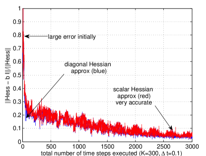
Figure 11: Accuracy of scalar Hessian approximation as a function of the optimization time steps. The relative error $\|\mathfrak{H}-\beta\mathbb{I}\|/\|\mathfrak{H}\|$, where $\beta$ is the average of the diagaonal elements of $\mathfrak{H}$, is quite large initially but the off-diagonal elements of $\mathfrak{H}$ quickly die off, and after only 3000 time steps (10 iterations at $K=300$ time steps per iteration), the relative error of the scalar approximation is on the order of 5%.

For small $\Delta t$ we can approximate the double integral

$$J_{mn}^{(k)}\approx\tfrac{1}{2}\Delta t^{2}U_{{\bf f}}(t_{k},\tau_{k})\{H_{m},H_{n}\}U_{{\bf f}}(\tau_{k},t_{k-1})$$ (48)

where $\tau_{k}=t_{k}-\tfrac{1}{2}\Delta t=t_{k-1}+\tfrac{1}{2}\Delta t$ and $\{H_{m},H_{n}\}=H_{m}H_{n}+H_{n}H_{m}$ is the anti-commutator, which yields

$$\mathfrak{H}_{mn}^{(k)}\approx-\tfrac{1}{2N}\Re\operatorname{Tr}\left(W^{\dagger}U_{{\bf f}}(T,\tau_{k})\{H_{m},H_{n}\}U_{{\bf f}}(\tau_{k},0)\right),$$

and if $W^{\dagger}U_{{\bf f}}(T,0)\approx\mathbb{I}$ then $W^{\dagger}U_{{\bf f}}(T,\tau_{k})\approx U_{{\bf f}}(\tau_{k},0)^{\dagger}$, thus cycling products under the trace, we obtain

$$\mathfrak{H}_{mn}^{(k)}\approx-\tfrac{1}{N}\Re\operatorname{Tr}(H_{m}H_{n}).$$ (49)

So if the control Hamiltonians $H_{m}$ are orthonormal with respect to the usual Hilbert-Schmidt inner product, i.e., $\operatorname{Tr}(H_{m}H_{n})=\delta_{mn}$ then we expect the Hessian $\mathfrak{H}^{(k)}$ to approach a multiple of the identity $-\tfrac{1}{N}\mathbb{I}$, at least for sufficiently small $\Delta t$ and fidelity sufficiently close to its maximum of $1$. In this limit the Newton update reduces to the greedy gradient update with the search length $\alpha_{\ast}$ based on a quadratic model of $F(\alpha)$ discussed in the previous section, since the gradient and Newton directions then coincide. Thus, if the local Hessian is close to a scalar matrix then evaluation and inversion of the Hessian simply adds extra computational overhead over the greedy gradient update. Furthermore, considering that the greedy gradient update is suboptimal globally, the Newton method may actually achieve worse convergence per iteration in the long run than the modified gradient update with overshoot, although the Newton method could be adapted to incorporate a scaling factor $\gamma$ to achieve a similar deliberate over- or undershoot effect.

These observations are confirmed by Fig. 9, showing that the sequential Newton update does not perform well in the long run for problem 1, which clearly satisfies $\operatorname{Tr}(H_{m}H_{n})=\delta_{mn}$. Close inspection shows that the Newton update outperforms the gradient update for the first few iterations, consistent with Fig. 11, which shows the relative error of the scalar Hessian approximation $\|\mathfrak{H}^{(k)}-\beta\mathbb{I}\|/\|\mathfrak{H}^{(k)}\|$ where $\beta$ here is the average of the diagonal elements of $\mathfrak{H}^{(k)}$, as the function of the total number of time steps executed. As expected, the scalar matrix approximation is a very poor fit initially but after approximately 3,000 time steps (10 iterations with $K=300$ time steps) the error of the scalar approximation is approximately 5%. Despite the fact that our time steps $\Delta t=0.1$ are not small ($\max|\omega_{nm}|\Delta t\not\leq 1$), and (48) is therefore not a very good approximation and the Hessian in the limit is not exactly diagonal, after a few iterations the diagonal elements are still sufficiently small to be negligible. This illustrates an important difference between approximating the gradient and Hessian — for both of these, it is the relative error which determines how accurate the step (44) will be, but contrary to the gradient, the Hessian does not tend to vanish at high fidelities, so that cruder approximations suffice to usefully estimate it.

The condition $\operatorname{Tr}(H_{m}H_{n})\propto\delta_{mn}$, implying $\mathfrak{H}^{(k)}\to\beta\mathbb{I}$ for gate optimization problems, is clearly satisfied for problems involving qubits or spin-$\tfrac{1}{2}$ particles with multiple independent local controls such as $X^{(n)}$, $Y^{(n)}$ or $Z^{(n)}$, and can always be made to hold by an application of the Gram-Schmidt orthonormalisation process to the control matrices. This argument does not apply however, to pure-state transfer, tracking or observable optimization problems, for which the Hessian in the limit can be arbitrary. For instance, if we consider the simplest case, $\mathfrak{F}_{1}({\bf f})=\Re\langle\Phi|\Psi_{{\bf f}}(T)\rangle$, then the local Hessian for the $k$th time slice, assuming $\Delta t$ not too large, is

$$\mathfrak{H}^{(k)}\approx\Re\langle\Phi|U_{{\bf f}}(T,\tau_{k})\{H_{m},H_{n}\}|\Psi_{{\bf f}}(\tau_{k})\rangle.$$ (50)

This expression will vanish for all $\tau_{k}$ and regardless of the initial and target state if $H_{m}$ and $H_{n}$ anti-commute, but in general it need not vanish even at the global maximum, and $\{H_{m},H_{n}\}=0$ for all $m,n>0$ is a much stronger condition than orthogonality, which is generally not even satisfied for spin systems with independent local controls on different qubits because e.g., $\{X^{(m)},X^{(n)}\}=2X^{(m)}X^{(n)}\neq 0$.

This suggests a dynamic choice of update rule depending on the type of problem considered. For gate optimization problems it may be useful to do a few trust-region update steps initially, possibly switching to a simplified Newton update as the Hessian approaches a diagonal matrix, before finally switching to a gradient update with a search length of $\frac{1}{N}$, or determined as described in the previous section. For other optimization problems such as state transfer or observable optimization, trust-region update is likely to be advantageous, although the added computational cost of evaluating the Hessian must be taken into account. This cost can be amortized, however, by exploiting the similarity between $\mathfrak{H}^{(k)}$ at adjacent $k$s for a given field along a sweep, and the fact that each $\mathfrak{H}^{(k)}$ individually converge as the field converges. Fig. 9 also suggests that sequential update algorithms initially lead to much larger gains in the fidelity than the most common concurrent update strategy based on a quasi-Newton algorithm with BFGS Hessian update de_fouquieres_second_2011 . However, the initial advantage of the sequential update diminshes as the optimization proceeds and the concurrent update overtakes the sequential varieties at high fidelities. The issue of comparison of sequential and concurrent update algorithms is explored in detail in machnes_comparing_2010 , which confirms this observation for a range of gate optimization problems, and suggests the development of hybrid strategies.

V Monotonicity and Rate of Convergence

If we allow the step size $s$ to be arbitrarily small, or in the extreme case let it vanish so that we are considering the instantaneous or continuous method, we have seen that analysis of the sequential scheme reduces to that of $\frac{\delta\mathfrak{F}({\bf f})}{\delta f_{m}(p)}$, because for all the fidelity functions we are considering, and even more generally, the fidelity varies in a linear fashion with respect to such local changes in the fields. Once we move to a fixed step size however, an accurate approximation to $\mathfrak{F}({\bf f}+\alpha b_{s}\mathbb{I}_{m})$ can require arbitrarily high order derivatives of $\mathfrak{F}$, and the most we can say in general regarding the $s\to 0$ regime is that the number of derivatives required to achieve a given accuracy for $\alpha$ scales as $1/s$. This is a weak result, however, which does not reveal much more than we had already established about different choices of $\alpha$. To get stronger results we need to distinguish at least two cases. The first is the unitary gate problem of $\mathfrak{F}_{7}$ or $\mathfrak{F}_{7b}$ and the second the pure state problem of $\mathfrak{F}_{1}$, which using the adjoint representation encompasses $\mathfrak{F}_{2}$ and therefore also $\mathfrak{F}_{5}$ and $\mathfrak{F}_{1b}$ as special cases of this latter. Contrary to the vanishing $s$ situation the analysis for finite step size $s$ is quite context sensitive and it is convenient to describe our results for the single control case before generalizing to several controls.

V.1 Quadratic Structure

Let us consider, at a given value of the single field $f$, how the fidelity $\mathfrak{F}|_{\alpha}:=\mathfrak{F}(f+\alpha b_{s,p_{k}})$ varies as the $f_{k}$ component of the field, corresponding to the basis function $b_{s,p_{k}}$, is changed by an amount $\alpha$. For all fidelity functions, integrating up the lower bound on their second derivative gives the quadratic lower bound

$$\mathfrak{F}|_{\alpha}\geq\mathfrak{F}(f)+\alpha\frac{\partial\mathfrak{F}(f)}{\partial f_{k}}+q\alpha^{2}$$ (51)

for $q$ equal to some global constant $q_{b}$. This immediately means any $\alpha$ between $0$ and $-\frac{1}{q_{b}}\frac{\partial\mathfrak{F}(f)}{\partial f_{k}}$ must lead to an increase in $\mathfrak{F}$, so that we have already identified a whole class of schemes monotonically increasing in $\mathfrak{F}$. In the unitary cases, what is interesting is that we can also find an upper bound of this form, with $q=q_{a}$, and such that $q_{a}\to q_{b}$ as $\mathfrak{E},s\to 0$. The actual fidelity along this local change in the field $\mathfrak{F}|_{\alpha}$ is therefore increasingly constrained as we approach the asymptotic instantaneous regime, so that an increase in $\mathfrak{F}$ can only happen for $\alpha$ between $0$ and $\frac{\partial\mathfrak{F}(f)}{\partial f_{k}}(\|H_{1}\|_{S}^{2}+O(\sqrt{\mathfrak{E}}+s))/s^{2}$. Over this $\alpha$ interval of interest, the difference between the bounds, therefore also the error incurred by the second order Taylor expansion of $\mathfrak{F}|_{\alpha}$ about $0$, is $\mathfrak{E}\,O(\sqrt{\mathfrak{E}}+s)$. More generally, in the unitary multiple control cases, we have that the local Hessian entries

$$\frac{\partial^{2}\mathfrak{F}(f)}{\partial f_{mk}\partial f_{nk}}=\frac{1}{s^{2}}[\operatorname{Tr}(H_{m}H_{n})+O(\sqrt{\mathfrak{E}}+s)],$$ (52)

and the error in the second order expansion of $\mathfrak{F}({\bf f})$ is still $\mathfrak{E}\,O(\sqrt{\mathfrak{E}}+s)$ for any change in ${\bf f}_{k}$ resulting in an increase of $\mathfrak{F}$.

This offers a classification of those $\alpha$ leading to monotonically increasing algorithms which coincides with the one of the previous section for fixed $\alpha$ and arbitrarily small $s$, but is also applicable to the practically relevant context with both $\alpha$ and $s$ fixed. It is also interesting to note that as $\mathfrak{F}|_{\alpha}$ is linear for arbitrarily small $s$, it is natural to add to it a purely quadratic cost term $\mathfrak{C}$ to ensure $\mathfrak{J}=\mathfrak{F}+\mathfrak{C}$ has a unique global maximum with respect to changes in $f$ by $b_{s}$ — but for $s$ fixed, such an alteration of the objective is inappropriate as it interferes with the already quadratic nature of $\mathfrak{F}|_{\alpha}$. In practice we also find that its second order Taylor expansion is a very good approximation to $\mathfrak{F}|_{\alpha}$ even when $s$ and especially $\mathfrak{E}$ are quite some distance away from the limiting value of $0$, and it therefore does not seem worth considering higher order expansions. Going beyond second order would also be quite problematic for more than one control as we would not have a reliable way of finding even local maxima based on this information.

V.2 Asymptotic Rate of Convergence

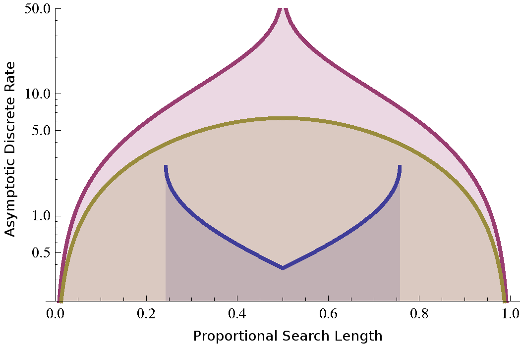
Figure 12: Static (red, above) and stateful (blue, below) bounds and static overestimate (yellow, in between) on the asymptotic rate of convergence for step size $s=\frac{\|H_{1}\|}{4\|[H_{1},H_{0}]\|}$. This is in the idealized case of $q_{a}=q_{b}$, but otherwise the left half of the figure would still be as shown with the proportional search length interpreted as $\alpha q_{b}$. The static bound is in fact infinite at $\frac{1}{2}$ since we cannot strictly rule out attaining a global maximum in a single step, but in practice it is standard to assume this can never happen, in which case the static overestimate gives an impression of what the bound would look like.

One guiding principle of numerical optimization is to be greedy: we wish to update the variables whenever enough information can be obtained to do so intelligently and aim to induce the largest possible increase in the objective. This would point towards back-and-forth sweeping, going to the maximum in ${\bf f}_{k}$ on each step, as the most efficient strategy as forward-only sweeping wastes the opportunity to increase the fidelity when propagating the backwards ODE. In the single field and unitary cases of the previous subsection the second order Taylor expansion generally provides a good estimate for the location of the maximum of $\mathfrak{F}|_{\alpha}$ closest to $0$, and using this $\alpha$ to update ${\bf f}_{k}$ gives a canonical optimization algorithm from the set of all possible strategies leading to a monotonic increase in the fidelity.

Unfortunately, as we have seen, this is not the best strategy as it is susceptible to rather extreme slowdown in the long run. The problem is that the fidelity is effectively quadratic and therefore going for the nearest maximum of fidelity is equivalent to making the local gradient as close to zero as possible. Moreover, as the Hessian converges to a fixed value in the limit the increase in fidelity achievable in this way is proportional to the gradient norm squared. Since the gradient $\frac{\partial\mathfrak{F}(f)}{\partial f_{k}}$ is the continuous function $\frac{\delta\mathfrak{F}(f)}{\delta f_{k}(t)}$ integrated against $b_{s,p_{k}}$, it cannot change much as we step to the next basis function $b_{s,p_{k+1}}$ centered at an adjacent point $p_{k+1}$, as is always the case for back-and-forth sweeping. Therefore taking the largest gains available on the current step, as with the canonical greedy algorithm, precludes large gains being made on subsequent steps. It is not immediately obvious, however, what the effect of this will be overall. To answer this question, we derive bounds on the rate of convergence, in particular the asymptotic rate, as we are already in the regime of small infidelity $\mathfrak{E}$ throughout. This stateful bound on the asymptotic rate of convergence is compared to the static bound in Fig. 12 for an illustrative choice of the step size $s$ and every valid search length $\alpha$. The combined bound reproduces the bimodal profile of asymptotic rate vs search length observed in Fig. 7 (right) — the rate must vanish towards the ends of the interval of search lengths making fidelity increase, but it must also be small for greedy search lengths in the middle of the interval.

In the remaining pure state, density matrix and observable cases, the situation is less decisive; in particular, the local Hessian need not converge to any predetermined value as $\mathfrak{E}$ and $s$ vanish. Naturally the fidelity with respect to local change in some ${\bf f}_{k}$ can only be accurately approximated up to the nearest local maximum by its second order Taylor expansion when the Hessian is not too small as otherwise this quadratic model does not even have a clear maximum. In the asymptotic instantaneous regime of small $\mathfrak{E}$ and $s$, however, we do have that when the Hessian is small, the local gradient must be too, implying that substantial increases in fidelity require large changes be made to ${\bf f}_{k}$. Our lack of certainty in the asymptotic local Hessian values precludes rigorously extending the clean picture from Fig. 12 to these cases, but the intuition behind it is equivalent. We must choose at each step between maximizing the immediate fidelity gain and restricting future gains by having a small gradient, and possibly introducing undesirably large peaks in the field by making large changes to the field amplitude.

V.3 General Rate Behavior

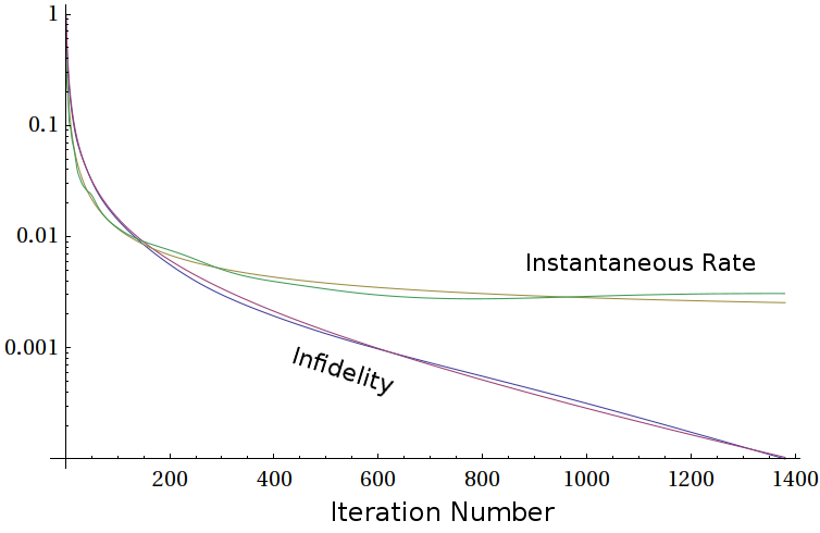
Figure 13: Combined plot of the infidelity and instantaneous rate across several sweeps comparing their actual and modelled values. The rate model is obtained by a two parameter least-squares fit of (53) to the rate data, which itself comes from forward differences of the infidelity logarithm. The infidelity model is based on the same $r^{\ast}$ and $r_{0}$, combined with a fitted value for the additional scale factor involved. The plotted run is the one with median sum of squares error in the infidelity model across a set of 100 runs.

In the asymptotic $\mathfrak{E}\to 0$ regime the behavior of discretized sequential optimization methods is determined by their linearization as discrete dynamical systems, independently of the specific objective or fidelity, number of controls, or type of sweep. This viewpoint motivates the following ansatz to describe the (instantaneous) rate of convergence at high fidelities:

$$r^{\ast}+\frac{1}{n}-\frac{r_{0}-r^{\ast}}{e^{n(r_{0}-r^{\ast})}-1}$$ (53)

where $n$ is the iteration number, $r^{\ast}$ the asymptotic rate and $(r^{\ast}+r_{0})/2$ the initial $n=0$ rate. Upon integration this provides a model for $\log(\mathfrak{E})$ up to a scale factor, and hence a model for $\mathfrak{F}$ with only $3$ parameters. While this model is motivated by analysis of the asymptotic regime it appears to approximate both the rate and fidelity remarkably accurately down to the first iteration as illustrated in Fig. 13.

VI Conclusions

In the context of quantum control, the method due to Krotov is usually presented in a continuous formulation and only discretized a posteriori for numerical use. However, we have seen how even the fundamental monotonicity property is jeopardized if the discretization scale $\Delta t$ is not taken into account when choosing the update rule. It is thus natural to view the discretized method, which is a sequentially updating optimization algorithm, as more fundamental and consider its continuous analogue as an instantaneous limit of this. The fidelity with respect to local changes in the field made in each step of such a sequential algorithm is essentially a quadratic function, which becomes linear in the instantaneous limit. Addition of a penalty in the continuous Krotov method can therefore be seen as a way of making the objective function quadratic, from which a canonical update formula emerges. Such a penalty is unnecessary for the discretized method, however, and in fact undesirable from both a theoretical and practical point of view.

At this stage a large class of monotonic update schemes with different sets of search lengths are available and in the literature the choice is typically left to the user. However, the search length is an important parameter that strongly influences the performance characteristics of the algorithm and guidance in selecting it is thus critical. The instrumental notion in doing so is the asymptotic rate of convergence, which had previously been shown salomon_convergence_2007 to be qualitatively at least linear, but for which no quantitative estimates were available. At first glance the natural choice of update scheme is the greedy one, maximizing immediate fidelity gains, but the asymptotic rate of convergence analysis shows that we cannot extrapolate from the initial rate of convergence, and proves this to be a poor strategy in the long run. Fortunately, the reason behind this failing also emerges from the analysis and we are able to offer modifications to the greedy search length or back-and-forth sweeping that enhance performance. The analysis explains why forward-only sweeping appears to be the preferred strategy in the literature, and suggests further improvements such as a split sweep that logically extend the advantage of forward-only over back-and-forth sweeping.

In discretizing the continuous method it is also common to use $\frac{\delta\mathfrak{F}}{\delta f(t_{k})}\Delta t$, where $\frac{\partial\mathfrak{F}}{\partial f_{k}}$ is the derivative in the instantaneous limit. However, this is only an approximation that is liable to break down and corrupt the algorithm, especially towards low infidelities $\mathfrak{E}$ or larger time steps $\Delta t$. We address this issue by outlining the exact method and various series expansions appropriate for computing these gradients $\frac{\partial\mathfrak{F}}{\partial f_{k}}$ for the most common choice of piecewise constant controls for each of the fidelity functionals under consideration. In selecting an update direction and search length one is naturally lead to use second derivative (Hessian) information, for which an exact formula is also available. In contrast to the situation for concurrent update optimization algorithms, the analysis also shows however that using the full local Hessian generally does not result in a performance improvement compared to a dynamic search length adjustment based on a quadratic model, at least for unitary gate optimization problems.

Looking forward, the general formulation of sequential methods applied to a wide range of control optimization problems that arise in the context of quantum control, as well as simplified convergence results should enable a streamlined application of these methods to optimizing other fidelity functions. The fact that any parametrization of the fields in terms of localized functions can be used for the sequential optimization opens the way for more problem-adapted choices than the standard top-hat function. Finally, the study of the convergence rate initiated herein should enable further development of heuristics to make more efficient choices of search lengths and sweeping patterns, and the development of hybrid methods that take advantage of the rapid improvements attainable by sequential update in the initial phase of the optimization to find suitable candidate fields with moderately high fidelities before switching to alternative strategies such as concurrent update to avoid the convergence slowdown of sequential update methods in the asymptotic regime. Taking together such improvements in the efficiency of the algorithms employed for dynamic control optimization should facilitate the application of the method to a wide range of coherent control problems and more realistic systems with larger Hilbert space dimensions or systems involving many qubits.

Appendix A Trust-Region Methods

The trust region sub-problem (TRSP) consists in finding a value of $x$ with $\|x\|\leq r$ such that $\frac{1}{2}x^{\mathrm{T}}Ax+g^{\mathrm{T}}x$ attains its minimum possible value over this ball of radius $r$. Since $A$ can always be taken symmetric, in a suitable eigenbasis, it can be expressed as a diagonal matrix with diagonal elements $\lambda_{1}\leq\lambda_{2}\ldots\leq\lambda_{n}$. We implicitly work in this basis in what follows, so in particular let $g_{1},\ldots,g_{n}$ be the components of the vector $g$ expressed in this basis. The key to solving this problem is finding the scalar $\mu^{\ast}\leq\min\{\lambda_{1},0\}$ such that $x_{\mu^{\ast}}$ defined by

$$x_{\mu}=-\left(A-\mu I\right)^{-1}g$$ (54)

has norm as close to $r$ as possible. If there exists $\mu_{*}$ such that $\|x_{\mu^{\ast}}\|=r$ then $x_{\mu^{\ast}}$ is the unique solution of the TRSP corresponding to a minimum at the boundary of the trust region. If $\|x_{\mu^{\ast}}\|<r$ and $\mu_{\ast}=0<\lambda_{1}$ then the unique solution of the TRSP is $x_{\mu_{\ast}}=-A^{-1}g$, corresponding to a minimum in the interior of the trust region. If $\|x_{\mu^{\ast}}\|<r$ but $\mu_{\ast}\leq\lambda_{1}<0$ then $e_{1}$ (the eigenvector corresponding to $\lambda_{1}$) is a direction of decrease and we can change the first component of $x_{\mu^{\ast}}$ (in the chosen eigenbasis) to reach norm $r$, and this point is a (not necessarily unique) solution to the TRSP corresponding to a minimum at the boundary.

To find $\mu^{\ast}$, one can find the roots of $\frac{1}{r}+\varphi(\mu)$, where

$$\varphi(\mu)=-\|x_{\mu}\|^{-1}=-\left(\sum_{k=1}^{n}\frac{g_{k}^{2}}{(\lambda_{k}-\mu)^{2}}\right)^{-1/2}.$$ (55)

As $\varphi$ is a convex increasing function for $\mu\leq\min\{\lambda_{1},0\}$ and its derivative $\varphi^{\prime}(\mu)=-\varphi(\mu)^{3}\sum_{k=1}^{n}\frac{g_{k}^{2}}{(\lambda_{k}-\mu)^{3}}$ is readily available, an efficient strategy is to use Newton root finding starting from $\mu_{0}=\min\left\{\lambda_{1},0\right\}$. If $\varphi\left(\mu_{0}\right)\leq-\frac{1}{r}$, then $\mu_{0}=\mu^{\ast}$. When $\mu_{0}=\lambda_{1}$ and $g_{1}\neq 0$ care must be taken to use $\varphi^{\prime}(\mu_{0})=\frac{1}{|g_{1}|}$.

Appendix B Convergence Results for Discretized Problem

As in the continuous case, convergence of the sequence $\{\mathfrak{F}^{(n)}\}$ (as a sequence of real numbers) is easy to establish provided (i) the objective functional $\mathfrak{F}({\bf f})$ is bounded above if we are maximizing, or below if we are minimizing, and (ii) the update scheme ensures monotonicity $\mathfrak{F}^{(n+1)}-\mathfrak{F}^{(n)}\geq 0$, as a monotonically increasing (decreasing) sequence of real numbers that is uniformly bounded above (below) is convergent. However, ideally we would like to know that we actually converge to a field ${\bf f}_{*}$ that is a critical point, and even better a global maximum (minimum) of the objective $\mathfrak{F}$. The latter convergence property is not a trivial matter since optimizing parameters sequentially can lead to iterates spiraling into a closed path without the gradient of the function converging to zero powell_search_1973 .

Sequential update schemes amount to iteratively updating a set of coordinates $\tilde{e}_{1},\ldots,\tilde{e}_{\tilde{K}}$ in a certain order. Specifically, we have $\tilde{K}=K$ and $\tilde{e}_{k}=e_{k}$ for forward-only update , $\tilde{K}=2(K-1)$ and $e_{1},\ldots,e_{K},\ldots,e_{2}$ for back-and-forth sweeping, and $\tilde{K}=K$ and $e_{1},\ldots,e_{\lfloor K/2\rfloor}$,$e_{K},\ldots,e_{\lfloor K/2\rfloor+1}$ for split update. In general $\tilde{e}_{n}$, equal to $\tilde{e}_{k}$ for $k\equiv n\operatorname{mod}\tilde{K}$, is the direction of the change between $x^{n}$ and $x^{n-1}$. In what follows, the full derivative is written $\mathrm{d}$, individual coordinates are referenced through subscripting, and we make use of the shorthand $\partial_{n}$ for the partial derivative in coordinate $\tilde{e}_{n+1}$.

Theorem 1

If we are sequentially maximizing an analytic function $F:\mathbb{R}^{K}\rightarrow\mathbb{R}$ with uniformly bounded second derivatives

$$\left|\frac{\partial^{2}F}{\partial x_{i}\partial x_{j}}\right|\leq\beta,$$ (56)

then we can obtain $F(x^{n+1})-F(x^{n})\geq\mu|\partial_{n}F(x^{n})|^{2}$ for $\mu=\frac{1}{2\beta}$ on each iteration. If this inequality holds for some $\mu$ and the lengths of our searches are forced to satisfy

$$|\tilde{x}^{n+1}_{n}-\tilde{x}^{n}_{n}|\leq\gamma|\partial_{n}F(x^{n})|$$ (57)

for some constant $\gamma$ then the sequence of iterates $x^{n}$ either diverges to infinity or converges to a stationary point.

Proof  To verify the first claim, suppose we vary the $i^{\operatorname{th}}$ coordinate. $-\beta\leq\tfrac{\partial^{2}F}{\partial x_{i}^{2}}$ over this line implies that $F$ is strictly increasing between $x$ and $x^{\prime}=x+\tfrac{1}{\beta}\tfrac{\partial F}{\partial x_{i}}e_{i}$ and the value of $F$ at $x^{\prime}$ is at least $F(x)+\frac{1}{2\beta}\left|\tfrac{\partial F}{\partial x_{i}}\right|^{2}$.

Next notice that updating $x^{n}$ along any coordinate can only alter the derivative $\tfrac{\partial F}{\partial x_{i}}$ by at most $\beta|\tilde{x}^{n+1}_{n}-\tilde{x}^{n}_{n}|\leq\beta\gamma|\partial_{n}F(x^{n})|$, so over several iterations we have

$$\left|\frac{\partial F}{\partial x_{i}}(x^{n})\right|\leq\left|\frac{\partial F}{\partial x_{i}}(x^{n+k})\right|+\sum_{j=0}^{k-1}\beta\gamma|\partial_{n+j}F(x^{n+j})|$$

for any non-negative $k$. Letting $k_{i}+1$ be the smallest index within $1,\ldots,\tilde{K}$ such that $\tilde{e}_{n+k_{i}+1}=e_{i}$, therefore

$$\|\mathrm{d}F(x^{n})\|_{1} \leq\sum_{i=1}^{K}\left|\partial_{n+k_{i}}F(x^{n+k_{i}})\right|+\sum_{j=0}^{k_{i}-1}\beta\gamma|\partial_{n+j}F(x^{n+j})|$$

$$\leq\sigma\sum_{j=0}^{\tilde{K}-1}|\partial_{n+j}F(x^{n+j})|$$

with $\sigma=1+(K-1)\beta\gamma$. Hence

$$F(x^{n+\tilde{K}})-F(x^{n})$$

$$\geq \sum_{j=0}^{\tilde{K}-1}\mu|\partial_{n+j}F(x^{n+j})|^{2}$$

$$\geq \frac{\mu}{\tilde{K}}\left(\sum_{j=0}^{\tilde{K}-1}|\partial_{n+j}F(x^{n+j})|\right)^{2}$$

$$\geq \frac{\mu}{\tilde{K}\sigma\gamma}\|\mathrm{d}F(x^{n})\|_{1}\sum_{j=0}^{\tilde{K}-1}|\tilde{x}^{n+j+1}_{n+j}-\tilde{x}^{n+j}_{n+j}|$$

$$\geq \frac{\mu}{\tilde{K}\sigma\gamma}\|\mathrm{d}F(x^{n})\|_{1}\|x^{n+\tilde{K}}-x^{n}\|_{1}$$

But this is exactly the primary descent condition of absil_convergence_2006 , and by the main result in this paper, the sequence $x^{n}$ either diverges, i.e., $\|x^{n}\|\rightarrow\infty$, or converges to some point $x^{\ast}$. In any case, if $F(x^{n})$ remains bounded we have

$$\sum_{n=0}^{\infty}|\partial_{n}F(x^{n})|^{2}\leq\frac{1}{\mu}\left(\underset{n\rightarrow\infty}{\lim}F(x^{n})-F(x^{0})\right)<\infty$$

implying $\partial_{n}F(x^{n})\rightarrow 0$ and by the earlier bound, $\|\mathrm{d}F(x^{n})\|\rightarrow 0$ as $n\rightarrow\infty$; in particular when $x^{\ast}$ exists, $\mathrm{d}F(x^{\ast})=0$. $\Box$

The same argument holds for objectives with or without a penalty term. However, if we add a standard weighted norm squared penalty term $\mathfrak{C}$, this norm of the controls is guaranteed to be uniformly bounded, so there is no way the controls can fail to converge at all.

References

- (1) V. May, D. Ambrosek, M. Oppel, and L. González, J. Chem. Phys. 127, 144102 (2007).
- (2) Y. Ohtsuki and Y. Fujimura, Chemical Physics 338, 285 (2007).
- (3) N. Doslić, K. Sundermann, L. González, O. Mó, J. Giraud-Girard, and O. Kühn, Phys. Chem. Chem. Phys. 1, 1249 (1999).
- (4) L. Wang, H. Meyer, and V. May, J. Chem. Phys. 125, 014102 (2006).
- (5) M. Ndong and C. P. Koch, Phys. Rev. A 82, 043437 (2010).
- (6) X. Wang, A. Bayat, S. Bose, and S. G. Schirmer, Phys. Rev. A 82, 012330 (2010).
- (7) X. Wang, A. Bayat, S. G. Schirmer, and S. Bose, Phys. Rev. A 81, 032312 (2010).
- (8) C. M. Tesch and R. de Vivie-Riedle, Phys. Rev. Lett. 89, 157901 (2002).
- (9) P. Treutlein, T. W. Hänsch, J. Reichel, A. Negretti, M. A. Cirone, and T. Calarco, Phys. Rev. A 74, 022312 (2006).
- (10) R. Nigmatullin and S. G. Schirmer, New J. Physics 11, 105032 (2009).
- (11) S. Schirmer, J. Mod. Opt. 56, 831 (2009).
- (12) C. P. Koch, J. P. Palao, R. Kosloff, and F. Masnou-Seeuws, Phys. Rev. A 70, 013402 (2004).
- (13) S. E. Sklarz and D. J. Tannor, Phys. Rev. A 66, 053619 (2002).
- (14) U. Hohenester, P. K. Rekdal, A. Borzì, and J. Schmiedmayer, Phys. Rev. A 75, 023602 (2007).
- (15) J. Grond, G. von Winckel, J. Schmiedmayer, and U. Hohenester, Phys. Rev. A 80, 053625 (2009).
- (16) M. Greiner, O. Mandel, T. Esslinger, T. W. Hansch, and I. Bloch, Nature 415, 39 (2002).
- (17) I. Bloch, J. Dalibard, and W. Zwerger, Rev. Mod. Phys. 80, 885 (2008).
- (18) D. Leibfried, R. Blatt, C. Monroe, and D. Wineland, Rev. Mod. Phys. 75, 281 (2003).
- (19) J. J. García-Ripoll, P. Zoller, and J. I. Cirac, Phys. Rev. Lett. 91, 157901 (2003).
- (20) J. J. García-Ripoll, P. Zoller, and J. I. Cirac, Phys. Rev. A 71, 062309 (2005).
- (21) U. Dorner, T. Calarco, P. Zoller, A. Browaeys, and P. Grangier, J. Opt. B 7, S341 (2005).
- (22) R. Blatt and D. Wineland, Nature 453, 1008 (2008).
- (23) M. Johanning, A. F. Varón, and C. Wunderlich, J. Phys. B 42, 154009 (2009).
- (24) C. Wunderlich, Nature 463, 37 (2010).
- (25) N. Timoney, V. Elman, S. Glaser, C. Weiss, M. Johanning, W. Neuhauser, and C. Wunderlich, Phys. Rev. A 77, 052334 (2008).
- (26) V. Nebendahl, H. Häffner, and C. F. Roos, Phys. Rev. A 79, 012312 (2009).
- (27) U. Hohenester and G. Stadler, Phys. Rev. Lett. 92, 196801 (2004).
- (28) E. Rasanen, A. Castro, J. Werschnik, A. Rubio, and E. K. U. Gross, Phys. Rev. Lett. 98, 157404 (2007).
- (29) A. Spörl, T. Schulte-Herbrüggen, S. J. Glaser, V. Bergholm, M. J. Storcz, J. Ferber, and F. K. Wilhelm, Phys. Rev. A 75, 012302 (2007).
- (30) P. Rebentrost, I. Serban, T. Schulte-Herbrüggen, and F. K. Wilhelm, Phys. Rev. Lett. 102, 090401 (2009).
- (31) M. Hofheinz, H. Wang, M. Ansmann, R. C. Bialczak, E. Lucero, M. Neeley, A. D. O’Connell, D. Sank, J. Wenner, J. M. Martinis, and A. N. Cleland, Nature 459, 546 (2009).
- (32) L. DiCarlo, J. M. Chow, J. M. Gambetta, L. S. Bishop, B. R. Johnson, D. I. Schuster, J. Majer, A. Blais, L. Frunzio, S. M. Girvin, and R. J. Schoelkopf, Nature 460, 240 (2009).
- (33) T. E. Skinner, T. O. Reiss, B. Luy, N. Khaneja, and S. J. Glaser, J. Magn. Res. 163, 8 (2003).
- (34) M. Ivanov, P. B. Corkum, T. Zuo, and A. Bandrauk, Phys. Rev. Lett. 74, 2933 (1995).
- (35) H. Niikura, F. Legare, R. Hasbani, A. D. Bandrauk, M. Y. Ivanov, D. M. Villeneuve, and P. B. Corkum, Nature 417, 917 (2002).
- (36) R. S. Judson and H. Rabitz, Physical Review Letters 68, 1500 (1992).
- (37) C. Daniel, J. Full, L. González, C. Lupulescu, J. Manz, A. Merli, Štefan Vajda, and L. Wöste, Science 299, 536 (2003).
- (38) T. Schulte-Herbrueggen, A. Spoerl, N. Khaneja, and S. J. Glaser, quant-ph/0609037 (2006).
- (39) M. Grace, C. Brif, H. Rabitz, I. A. Walmsley, R. L. Kosut, and D. A. Lidar, J. Phys. B 40, S103 (2007).
- (40) J. Somloi, V. A. Kazakov, and D. J. Tannor, Chem. Phys. 172, 85 (1993).
- (41) W. Zhu and H. Rabitz, J. Chem. Phys. 109, 385 (1998).
- (42) Y. Maday and G. Turinici, J. Chem. Phys. 118, 8191 (2003).
- (43) W. Zhu, J. Botina, and H. Rabitz, J. Chem. Phys. 108, 1953 (1998).
- (44) Y. Ohtsuki, W. Zhu, and H. Rabitz, J. Chem. Phys. 110, 9825 (1999).
- (45) J. P. Palao and R. Kosloff, Phys. Rev. Lett. 89, 188301 (2002).
- (46) J. P. Palao and R. Kosloff, Phys. Rev. A 68, 062308 (2003).
- (47) Y. Ohtsuki, G. Turinici, and H. Rabitz, J. Chem. Phys. 120, 5509 (2004).
- (48) J. Salomon, in IEEE Conf. Decision & Control (IEEE, ADDRESS, 2005), Vol. 44, p. 5854.
- (49) D. Reich, M. Ndong, and C. P. Koch, arXiv:1008.5126 (2010).
- (50) P. de Fouquieres, S. G. Schirmer, S. J. Glaser, and I. Kuprov, arXiv:1102.4096 (2011).
- (51) S. Machnes, U. Sander, S. J. Glaser, P. de Fouquieres, A. Gruslys, S. Schirmer, and T. Schulte-Herbrueggen, arXiv:1011.4874 (2010).
- (52) J. Salomon, Mathematical Modelling & Numerical Analysis 41, 77 (2007).
- (53) M. J. D. Powell, Mathematical Programming 4, 193 (1973).
- (54) P. A. Absil, R. Mahony, and B. Andrews, SIAM J. Optim. 16, 531 (2006).