High-Dimensional Topological Insulators with Quaternionic Analytic Landau Levels

Abstract

We study the 3D topological insulators in the continuum by coupling spin-$\frac{1}{2}$ fermions to the Aharonov-Casher SU(2) gauge field. They exhibit flat Landau levels in which orbital angular momentum and spin are coupled with a fixed helicity. The 3D lowest Landau level wavefunctions exhibit the quaternionic analyticity as a generalization of the complex analyticity of the 2D case. Each Landau level contributes one branch of gapless helical Dirac modes to the surface spectra, whose topological properties belong to the $\mathbb{Z}_{2}$-class. The flat Landau levels can be generalized to an arbitrary dimension. Interaction effects and experimental realizations are also studied.

The 2D quantum Hall (QH) systems Klitzing1980 ; tsui1982 are among the earliest examples of quantum states characterized by topology thouless1982 ; haldane1988 rather than symmetry in condensed matter physics. Their magnetic band structures possess topological Chern numbers defined in time-reversal (TR) symmetry breaking systems thouless1982 ; avron1983 ; niu1985 ; kohmoto1985 ; avron1990 . The consequential quantized charge transport originates from chiral edge modes laughlin1981 ; halperin1982 , a result from the chirality of Landau level wavefunctions. Current studies of TR invariant topological insulators (TIs) have made great success in both 2D and 3D. They are described by a $\mathbb{Z}_{2}$-invariant which is topologically stable with respect to TR invariant perturbations bernevig2006a ; kane2005 ; kane2005a ; fu2007 ; fu2007a ; moore2007 ; bernevig2006 ; qi2008 ; roy2009 ; roy2010 ; hasan2010 ; qi2011 . On open boundaries, they exhibit odd numbers of gapless helical edge modes in 2D systems and surface Dirac modes in 3D systems. TIs have been experimentally observed through transport experiments konig2007 ; qu2010 ; xiong2012 and spectroscopic measurements roushan2009 ; hsieh2008 ; hsieh2009 ; xia2009 ; chen2009 ; alpichshev2010 ; zhang2009a .

The current research of 3D TIs has been focusing on the Bloch-wave band structures. Nevertheless, Landau levels (LLs) possess the advantages of the elegant analytic properties and flat spectra, both of which have played essential roles in the study of 2D integer and fractional QH effects laughlin1983 ; Haldane1983 ; halperin1984 ; girvin1984 ; arovas1984 ; haldane1985 ; girvin1987 ; jain1989 ; jain2007 ; zhang1989 ; moore1991 ; wen1992 ; sondhi1993 ; murthy2003 ; DasSarma2005 ; DasSarma2008 . As pioneered by Zhang and Hu zhang2001 , LLs and QH effects have been generalized to various high dimensional manifolds zhang2001 ; bernevig2002 ; elvang2003 ; fabinger2002 ; bernevig2003 ; hasebe2010 . However, to our knowledge, TR invariant isotropic LLs have not been studied in 3D flat space before. It would be interesting to develop the LL counterpart of 3D TIs in the continuum independent of the band inversion mechanism. The analytic properties of 3D LL wavefunctions and the flatness of their spectra provide an opportunity for further investigation on non-trivial interaction effects in 3D topological states.

In this Letter, we construct 3D isotropic flat LLs in which spin-$\frac{1}{2}$ fermions are coupled to an $SU(2)$ Aharonov-Casher potential. When odd number LLs are fully filled, the system is a 3D $\mathbb{Z}_{2}$ TI with TR symmetry. Each LL state has the same helicity structure, i.e., the relative orientation between orbital angular momentum and spin. Just like that the 2D lowest LL (LLL) wavefunctions in the symmetric gauge are complex analytic functions, the 3D LLL ones are mapped into quaternionic analytic functions. Different from the 2D case, there is no magnetic translational symmetry for the 3D LL Hamiltonian due to the non-Abelian nature of the gauge field. Nevertheless, magnetic translations can be applied for the Gaussian pocket-like localized eigenstates in the LLL. The edge spectra exhibit gapless Dirac modes. Their stability against TR invariant perturbations indicates the $\mathbb{Z}_{2}$ nature. This scheme can be easily generalize to $N$ dimensions. Interaction effects and the Laughlin-like wavefunctions for the 4D case are constructed. Realizations of the 3D LL system are discussed.

We begin with the 3D LL Hamiltonian for a spin-$\frac{1}{2}$ non-relativistic particle as

$$H^{3D,LL}=\frac{1}{2m}\sum_{a}\big{\{}-i\hbar\nabla^{a}-\frac{q}{c}A^{a}(\vec{r})\big{\}}^{2}+V(r),$$ (1)

where $A^{a}_{\alpha\beta}=\frac{1}{2}G\epsilon_{abc}\sigma_{\alpha\beta}^{b}r^{c}$ is a 3D isotropic $SU(2)$ gauge with Latin indices run over $x,y,z$ and Greek indices denote spin components $\uparrow,\downarrow$; $G$ is a coupling constant and $\sigma$’s are Pauli matrices; $V(r)=-\frac{1}{2}m\omega_{0}^{2}r^{2}$ is a harmonic potential with $\omega_{0}=|qG|/(2mc)$ to maintain the flatness of LLs. $\vec{A}$ can be viewed as an Aharonov-Casher potential associated with a radial electric field linearly increasing with $r$ as $\vec{E}(r)\times\vec{\sigma}$. $H^{3D,LL}$ preserves the TR symmetry in contrast to the 2D QH with TR symmetry broken. It also gives a 3D non-Abelian generalization of the 2D quantum spin Hall Hamiltonian based on Landau levels studied in Ref. bernevig2006a . More explicitly, $H^{3D,LL}$ can be further expanded as a harmonic oscillator with a constant spin-orbit (SO) coupling as

$$H^{3D,LL}_{\mp}=\frac{p^{2}}{2m}+\frac{1}{2}m\omega_{0}^{2}r^{2}\mp\omega_{0}\vec{\sigma}\cdot\vec{L},$$ (2)

where $\mp$ apply to the cases of $qG>0~{}(<0)$, respectively. The spectra of Eq. 2 were studied in the context of the supersymmetric quantum mechanics bagchi2001 . However, its connection with Landau levels was not noticed. Eq. 1 has also been proposed to describe the electrodynamic properties of superconductors hirsch2008 ; hirsch2008a ; hirsch2013 .

The spectra and eigenstates of Eq. 1 are explained as follows. We introduce the helicity number for the eigenstate of $\vec{L}\cdot\vec{\sigma}$, defined as the sign of its eigenvalue of the total angular momentum $\vec{J}=\vec{L}+\vec{S}$, which equals $\pm 1$ for the sectors of $j_{\pm}=l\pm\frac{1}{2}$, respectively. At $qG>0$, the eigenstates are denoted as $\psi_{n_{r};j_{\pm},j_{z};l}(\vec{r})=R_{n_{r},l}(r)\mathcal{Y}_{j_{\pm},j_{z};l}(\hat{\Omega})$, where the radial function is $R_{n_{r}l}(r)=r^{l}e^{-\frac{r^{2}}{4l_{G}^{2}}}F(-n_{r},l+\frac{3}{2},\frac{r^{2}}{2l_{G}^{2}})$; $F$ is the confluent hypergeometric function and $l_{G}=\sqrt{\frac{\hbar c}{qG}}$ is the analogy of the magnetic length; $\mathcal{Y}_{j_{\pm},j_{z};l}(\hat{\Omega})$’s are the spin-orbit coupled spheric harmonic with $j_{\pm}=l\pm\frac{1}{2}$, respectively. Flat spectra appear with infinite degeneracy in the sector of $j_{+}$, where the energy dispersion $E_{n_{r},l}^{+}=(2n_{r}+\frac{3}{2})\hbar\omega_{0}$ is independent of $l$, and thus $n_{r}$ serves as the LL index. For the sector of $j_{-}$, the energy disperses with $l$ as $E_{n_{r},l}^{-}=[2(n_{r}+l)+\frac{5}{2}]\hbar\omega_{0}$. Similar results apply to the case of $qG<0$, where the infinite degeneracy occurs in the sector of $j_{-}$. These LL wavefunctions are the same as those of the 3D harmonic oscillator but with different organizations. As illustrated in Fig. 1 (a), these eigenstates along each diagonal line with the positive (negative) helicity fall into the flat LL states for the case of $qG>0~{}(<0)$, respectively. The ladder algebra generating the whole 3D LL states is explained in the Supplemental Material suppl .

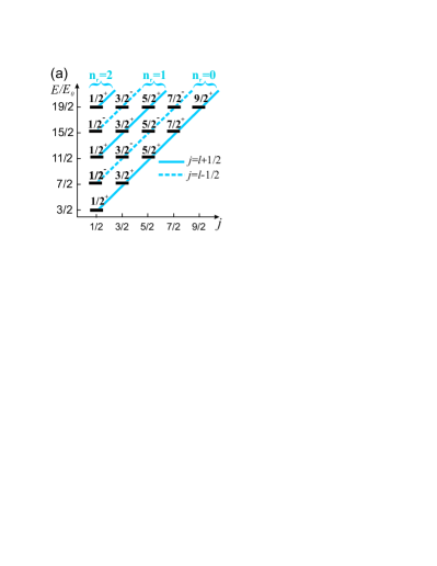
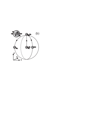
Figure 1: a) The eigenstates of the 3D harmonic oscillator labeled by total angular momentum $j_{\pm}=l\pm\frac{1}{2}$. Following the solid diagonal (dashed) lines, these states are reorganized into the 3D LL sates with the positive (negative) helicity. b) The magnetic translation for the LLL state ($l=0$) localized at the origin in the case of $qG>0$, whose spin is set along an arbitrary direction in the $xy$-plane. The displacement vector $\vec{\delta}$ lies in the plane perpendicular to spin orientation. The resultant state remains in the LLL as a localized Gaussian pocket.

Compared to the 2D case, a marked difference is that the 3D LL Hamiltonian has no magnetic translational symmetry. The non-Abelian field strength grows quadratically with $r$ as $F_{ij}(\vec{r})=\partial_{i}A_{j}-\partial_{j}A_{i}-\frac{iq}{\hbar c}[A_{i},A_{j}]=g\epsilon_{ijk}\big{\{}\sigma^{k}+\frac{1}{4l_{G}^{2}}r^{k}(\vec{\sigma}\cdot\vec{r})\big{\}}$. Nevertheless, magnetic translations still apply to the highest weight states of the total angular momentum $\vec{J}=\vec{L}+\vec{S}$ in the LLL at $qG>0$. For simplicity, we drop the normalization factors of wavefunctions below. For the positive helicity states with $j_{z}=j_{+}$, $\vec{L}$ and $\vec{S}$ are parallel to each other. Their wavefunctions are denoted by $\psi_{\hat{z},l}^{hw}(\vec{r})=(x+iy)^{l}e^{-\frac{r^{2}}{4l_{G}^{2}}}\otimes\alpha_{\hat{\Omega}=\hat{z}}$, where $\alpha_{\hat{\Omega}}$ is the spin eigenstate of $\hat{\Omega}\cdot\vec{\sigma}$ with eigenvalue $1$. For these states, the magnetic translation is defined as usual $T_{\hat{z}}(\vec{\delta})=\exp[-\vec{\delta}\cdot\vec{\nabla}+\frac{i}{4l_{G}^{2}}\vec{r}_{xy}\cdot(\hat{z}\times\vec{\delta})]$, where $\vec{\delta}$ is the displacement vector in the $xy$-plane and $\vec{r}_{xy}$ is the projection of $\vec{r}$ in the $xy$-plane. The resultant state, $T_{\hat{z}}(\vec{\delta})\psi_{\hat{z},l}^{hw}(\vec{r})=e^{i\frac{\vec{r}_{xy}\cdot(\hat{z}\times\delta)}{4l_{G}^{2}}}\psi_{\hat{z},l}^{hw}(\vec{r}-\vec{\delta})$, remains in the LLL. Generally speaking, the highest weight states can be defined in a plane spanned by two orthogonal unit vectors $\hat{e}_{1,2}$ as $\psi_{\hat{e}_{3},l}^{hw}(\vec{r})=[(\hat{e}_{1}+i\hat{e}_{2})\cdot\vec{r}]^{l}e^{-\frac{r^{2}}{4l_{G}^{2}}}\otimes\alpha_{\hat{e}_{3}}$ with $\hat{e}_{3}=\hat{e}_{1}\times\hat{e}_{2}$. The magnetic translation for such states is defined as $T_{\hat{e}_{3}}(\vec{\delta})=\exp[-\vec{\delta}\cdot\vec{\nabla}+\frac{i}{4l_{G}^{2}}~{}\vec{r}_{12}\cdot(\hat{e}_{3}\times\vec{\delta})]$, where $\vec{\delta}$ lies in the $\hat{e}_{1,2}$-plane and $\vec{r}_{12}=\vec{r}-\hat{e}_{3}(\vec{r}\cdot\hat{e}_{3})$. As an example, let us translate the LLL state localized at the origin as illustrated in Fig. 1 (b). We set the spin direction of $\psi^{LLL}_{\hat{e}_{3},l=0}$ in the $xy$-plane parameterized by $\hat{e}_{3}(\gamma)=\hat{x}\cos\gamma+\hat{y}\sin\gamma$, i.e., $\alpha_{\hat{e}_{3}}(\gamma)=\frac{1}{\sqrt{2}}(|\uparrow\rangle+e^{i\gamma}|\downarrow\rangle)$, and translate it along $\hat{e}_{1}=\hat{z}$ at the distance $R$. The resultant states read as

$$\psi_{\gamma,R}(\rho,\phi,z)=e^{i\frac{g}{2}R\rho\sin(\phi-\gamma)}e^{-|\vec{r}-R\hat{z}|^{2}/4l_{G}^{2}}\otimes\alpha_{\hat{e}_{3}}(\gamma),$$ (3)

where $\rho=\sqrt{x^{2}+y^{2}}$ and $\phi$ is the azimuthal angular of $\vec{r}$ in the $xy$-plane. Such a state remains in the LLL as an off-centered Gaussian wave packet.

The highest weight states and their descendent states from magnetic translations defined above have a clear classic picture. The classic equations of motion are derived as

$$\dot{\vec{r}} = \frac{1}{m}\vec{p}+2\omega_{0}(\vec{r}\times\frac{1}{\hbar}\vec{S}),\ \ \,\dot{\vec{p}}=2\omega_{0}\vec{p}\times\frac{1}{\hbar}\vec{S}-m\omega_{0}^{2}\vec{r},$$

$$\dot{\vec{S}} = \frac{2\omega_{0}}{\hbar}\vec{S}\times\vec{L},$$ (4)

where $\vec{p}$ is the canonical momentum, $\vec{L}=\vec{r}\times\vec{p}$ is the canonical orbital angular momentum, and $\vec{S}$ here is the expectation value of $\frac{\hbar}{2}\vec{\sigma}$. The first two describe the motion in a non-inertial frame subject to the angular velocity $\frac{2\omega_{0}}{\hbar}\vec{S}$, and the third equation is the Larmor precession. $\vec{L}\cdot\vec{S}$ is a constant of motion of Eq. 4. In the case of $\vec{S}\parallel\vec{L}$, it is easy to prove that both $\vec{S}$ and $\vec{L}$ are conserved. Then the cyclotron motions become coplanar within the equatorial plane perpendicular to $\vec{S}$. Centers of the circular orbitals can be located at any points in the plane.

The above off-centered LLL states break all the rotational symmetries. Nevertheless, we can recover the rotational symmetry around the axis determined by the origin and the packet center. Let us perform the Fourier transform of $\psi_{\gamma,R}(\rho,\phi,z)$ in Eq. 3 with respect to the azimuthal angle $\gamma$ of spin polarization. The resultant state, $\psi_{j_{z}=m+\frac{1}{2},R}(\rho,\phi,z)=\int_{0}^{2\pi}\frac{d\gamma}{2\pi}e^{im\gamma}\psi_{\gamma,R}$, is a $j_{z}$-eigenstate as

$$e^{\frac{-|\vec{r}-R\hat{z}|^{2}}{4l_{G}^{2}}}e^{im\phi}\Big{\{}J_{m}(x)|\uparrow\rangle+J_{m+1}(x)e^{i\phi}|\downarrow\rangle\Big{\}},$$ (5)

with $x=R\rho/(2l_{G}^{2})$. At large distance of $R$, the spatial extension of $\psi_{j_{z}=m+\frac{1}{2},R}$ in the $xy$-plane is at the order of $ml_{G}^{2}/R$, which is suppressed at large values of $R$ and scales linear with $m$. In particular, the narrowest states $\psi_{\pm\frac{1}{2},R}$ exhibit an ellipsoid shape with an aspect ratio decaying as $l_{G}/R$ when $R$ goes large.

In analogy to the fact that the 2D LLL states are complex analytic functions due to chirality, we have found an impressive result that the helicity in 3D LL systems leads to the quaternionic analyticity. Quaternion is the first discovered non-commutative division algebra, which has three anti-commuting imaginary units $i$, $j$ and $k$, satisfying $i^{2}=j^{2}=k^{2}=-1$ and $ij=k$. It has been applied in quantum systems Balatsky1992 ; adler1995 and SO coupled Bose-Einstein condensations li2012b . Just like two real numbers forming a complex number, a two-component complex spinor $\psi=(\psi_{\uparrow},\psi_{\downarrow})^{T}$ can be viewed as a quaternion defined as $f=\psi_{\uparrow}+j\psi_{\downarrow}$. In the quaternion representation, the TR transformation $i\sigma_{2}\psi^{*}$ becomes $Tf=-fj$ satisfying $T^{2}=-1$; multiplying a U(1) phase factor $e^{i\phi}\psi$ corresponds to $fe^{i\phi}$; the SU(2) operations $e^{-i\frac{\sigma_{x}}{2}\phi}\psi$, $e^{-i\frac{\sigma_{y}}{2}\phi}\psi$, and $e^{-i\frac{\sigma_{z}}{2}\phi}\psi$ map to $e^{\frac{k}{2}\phi}f$, $e^{\frac{j}{2}\phi}f$, and $e^{-\frac{i}{2}\phi}f$, respectively. The quaternion version of $\psi^{LLL}_{j=j_{+},j_{z}=m+\frac{1}{2}}$ is $f_{j_{+},j_{z}}^{LLL}(x,y,z)=\Psi_{\uparrow,j_{+},j_{z}}+j\Psi_{\downarrow,j_{+},j_{z}}$, where $\Psi_{\uparrow,j_{+},j_{z}}=\langle j_{+},j_{z}|l,m;\frac{1}{2},\frac{1}{2}\rangle r^{l}Y_{l,m}$, $\Psi_{\downarrow,j_{+},j_{z}}=\langle j_{+},j_{z}|l,m+1;\frac{1}{2},-\frac{1}{2}\rangle r^{l}Y_{l,m+1}$. Please note that the Gaussian factor does not appear in $f_{j_{+},j_{z}}^{LLL}$ which is a quaternionic polynomial.

As a generalization of the Cauchy-Riemann condition, a quaternionic analytic function $f(x,y,z,u)$ satisfies the Fueter condition sudbery1979 as

$$\frac{\partial f}{\partial x}+i\frac{\partial f}{\partial y}+j\frac{\partial f}{\partial z}+k\frac{\partial f}{\partial u}=0,$$ (6)

where $x$, $y$, $z$ and $u$ are coordinates in the 4D space. In Eq. 6, imaginary units are multiplied from the left, thus it is the left-analyticity condition which works in our convention. Below, we prove the LLL function $f_{j_{+},j_{z}}^{LLL}(x,y,z)$ satisfying Eq. 6. Since $f_{j_{+},j_{z}}^{LLL}$ is defined in 3D space, it is a constant over $u$, and thus only the first three terms in Eq. 6 apply to it. Obviously the highest weight states with spin along the $z$-axis, $f^{LLL}_{j_{+}=j_{z}=l+\frac{1}{2}}=(x+iy)^{l}$, satisfy Eq. 6 which is reduced to complex analyticity. By applying an arbitrary SU(2) rotation $g$ characterized by the Eulerian angles $(\alpha,\beta,\gamma)$, $f^{LLL}_{j_{+}=j_{z}}$ transforms to

$$f^{\prime,~{}LLL}(x,y,z)=e^{-i\frac{\alpha}{2}}e^{j\frac{\beta}{2}}e^{-i\frac{\gamma}{2}}f^{LLL}_{j_{+}=j_{z}}(x^{\prime},y^{\prime},z^{\prime}),$$ (7)

where $(x^{\prime},y^{\prime}$, $z^{\prime})$ are the coordinates by applying the inverse of $g$ on $(x,y,z)$. We check that $(\frac{\partial}{\partial x}+i\frac{\partial}{\partial y}+j\frac{\partial}{\partial z})f^{\prime LLL}(x,y,z)=e^{i\frac{\alpha}{2}}e^{-j\frac{\beta}{2}}e^{i\frac{\gamma}{2}}\Big{\{}\frac{\partial}{\partial x^{\prime}}+i\frac{\partial}{\partial y^{\prime}}+j\frac{\partial}{\partial z^{\prime}}\Big{\}}f^{LLL}_{j_{+},j_{z}}(x^{\prime},y^{\prime},z^{\prime})=0$. Essentially, we have proved that Fueter condition is rotationally invariant. Since all the highest weight states are connected through SU(2) rotations, and they form an over-complete basis for the angular momentum representations, we conclude that all the 3D LLL states with the positive helicity are quaternionic analytic.

Next we prove that the set of quaternionic LLL states $f^{LLL}_{j_{+}=l+\frac{1}{2},j_{z}}$form the complete basis for quaternionic valued analytic polynomials in 3D. Any linear superposition of the LLL states with $j_{+}$ can be represented as $f_{l}=\sum_{j_{z}=-j_{+}}^{j_{+}}f^{LLL}_{j_{+},j_{z}}~{}c_{j_{z}}$, where $c_{j_{z}}$ is a complex coefficient. Because of the TR relation $f^{LLL}_{j_{+},-j_{z}}=-f^{LLL}_{j_{+},-j_{z}}j$, $f_{l}$ can be expressed in terms of $l+1$ linearly independent basis as

$$f_{l}(x,y,z)=\sum_{m=0}^{l}f^{LLL}_{j_{+}=l+\frac{1}{2},j_{z}=m+\frac{1}{2}}q_{m},$$ (8)

where $q_{m}=c_{m+\frac{1}{2}}-jc_{-m-\frac{1}{2}}$ is a quaternion constant. On the other hand, it can be calculated that the rank of the linearly independent $l$-th order quaternionic polynomials satisfying Eq. 6 is just $C^{2}_{l+2}-C^{2}_{l+1}=l+1$, thus $f^{LLL}_{j_{+},j_{z}}$’s with $j_{z}\geq\frac{1}{2}$ are complete.

The topological nature of the 3D LL problem exhibits clearly in the gapless surface states. A numeric calculation of the gapless surface spectra is presented in the Supplemental Material suppl . At $qG>0$, inside the bulk, LL spectra are flat with respect to $j_{+}=l+\frac{1}{2}$. As $l$ goes large, the classical orbital radius $r_{c}$ approaches the open boundary with the radius $R_{0}$. For example, for a LLL state, $r_{c}=\sqrt{2l}l_{G}$. States with $l>l_{c}\approx\frac{1}{2}(R_{0}/l_{G})^{2}$ become surface states. Their spectra become $E(l)\approx l(l+1)\frac{\hbar^{2}}{2mR_{0}^{2}}-l\hbar\omega_{0}$. When the chemical potential $\mu$ lies inside the gap, it cuts the surface states with the Fermi angular momentum denoted by $l_{f}$. These surface states satisfy $\vec{\sigma}\cdot\vec{L}=l\hbar$, thus the their spectra can be linearized around $l_{f}$ as $H_{bd}=(v_{f}/R_{0})\vec{\sigma}\cdot\vec{L}-\mu$. This is the Dirac equation defined on a sphere with the radius $R_{0}$. It can be expanded around $\vec{r}=R_{0}\hat{e}_{r}$ as $H_{bd}=\hbar v_{f}(\vec{k}\times\vec{\sigma})\cdot\hat{e}_{r}-\mu$. Similar reasoning applies to other Landau levels which also give rise to Dirac spectra. Because of the lack of Bloch wave band structure, it remains a challenging problem to directly calculate the bulk topological index. Nevertheless, the $\mathbb{Z}_{2}$ structure manifests through the surface Dirac spectra. Since each fully occupied LL contributes one helical Dirac Fermi surface, the bulk is $\mathbb{Z}_{2}$-nontrivial (trivial) if odd (even) number of LLs are occupied. In the $\mathbb{Z}_{2}$-nontrivial case, the gapless helical surface states are protected by TR symmetry and are robust under TR invariant perturbations.

In Eq. 2, the harmonic frequency $\omega_{T}$ is set to be equal with the SO frequency $\omega_{0}$ to maintain the flatness of LL spectra. However, the $\mathbb{Z}_{2}$ topology of the 3D LLs does not rely on this. Define $\Delta\omega=\omega_{T}-\omega_{0}$, and we set $\Delta\omega\geq 0$ to maintain the spectra bounded from below. $\Delta\omega>0$ corresponds to imposing an external potential $\Delta V(r)=\frac{1}{2}m(\omega_{T}^{2}-\omega_{0}^{2})r^{2}$ to the bulk Hamiltonian of Eq. 2. If $\Delta\omega\ll\omega_{0}$, $\Delta V(r)$ is soft. It results in energy dispersions of 3D LLs but does not affect their topology. For simplicity, let us check the case of $qG>0$. The $\vec{\sigma}\cdot\vec{L}$ term commutes with the overall harmonic potential, thus the LL wavefunctions remain the same as those of Eq. 2 by replacing $\omega_{0}$ with $\omega_{T}$. Their dispersions become $E^{+}_{n_{r},j_{+}}=(2n_{r}+1)\hbar\omega_{T}+\frac{1}{2}\hbar\omega_{0}+j_{+}\hbar\Delta\omega$ which are very slow. In other words, $\Delta V(r)$ imposes a finite sample size with the radius of $R^{2}<\hbar/(m\Delta\omega)=2l_{G}\frac{\omega_{0}}{\Delta\omega}$ even without an explicit boundary. Inside this region, $\Delta V$ is smaller than the LL gap, and the LL states are bulk states. Their energies are within the LL gap and the angular momentum numbers $j_{+}<\frac{2\omega_{T}}{\Delta\omega}$. LL states outside this region can be viewed as surface states with positive helicity. For a given Fermi energy, it also cuts a helical Fermi surface with the same form of effective surface Hamiltonian.

The above scheme can be easily generalized to arbitrary dimensions suppl by combining the $N$-D harmonic oscillator potential and SO coupling. For example, in 4D, we have $H^{4D,LL}=\frac{p_{4D}^{2}}{2m}+\frac{1}{2}m\omega_{0}^{2}r_{4D}^{2}-\omega_{0}\sum_{1\leq a<b\leq 4}\Gamma^{ab}L_{ab}$, where $L_{ab}=r_{a}p_{b}-r_{b}p_{a}$ and the 4D spin operators are defined as $\Gamma^{ij}=-\frac{i}{2}[\sigma^{i},\sigma^{j}]$, $\Gamma^{i4}=\pm\sigma^{i}$ with $1\leq i<j\leq 3$. The $\pm$ signs of $\Gamma^{i4}$ correspond to two complex conjugate irreducible fundamental spinor representations of $SO(4)$, and the $+$ sign will be taken below. The spectra of the positive helicity states are flat as $E_{+,n_{r}}=(2n_{r}+2)\hbar\omega$. Following a similar method in 3D, we prove that the quaternionic version of the 4D LLL wavefunctions satisfy the full equation of Eq. 6. They form the complete basis for quaternionic left-analytic polynomials in 4D. For each $l$-th order, the rank can be calculated as $C^{3}_{l+3}-C^{3}_{l+2}=\frac{1}{2}(l+1)(l+2)$.

We consider the interaction effects in the LLLs. For simplicity, let us consider the 4D system and the short-range interactions. Fermions can develop spontaneous spin polarization to minimize the interaction energy in the LLL flat band. Without loss of generality, we assume that spin takes the eigenstate of $\Gamma^{12}=\Gamma^{34}=\sigma^{3}$ with the eigenvalue 1. The LLL wavefunctions satisfying this spin polarization can be expressed as $\Psi^{LLL,4D}_{m,n}=(x+iy)^{m}(z+iu)^{n}e^{-\frac{r^{2}_{4D}}{4l_{G}^{c}2}}\otimes|\alpha\rangle$ with $|\alpha\rangle=(1,0)^{T}$. The 4D orbital angular momentum number for the orbital wavefunction is $l=m+n$ with $m\geq 0$ and $n\geq 0$. It is easy to check that $\Psi^{LLL,4D}_{m,n}$ is the eigenstate of $\sum_{ab}L_{ab}\Gamma^{ab}$ with the eigenvalue $(m+n)\hbar$. If all the $\Psi^{LLL,4D}_{m,n}$’s are filled with $0\leq m<N_{m}$ and $0\leq n<N_{n}$, we write down a Slater-determinant wavefunction as

$$\Psi(v_{1},w_{1};\cdots;v_{N},w_{N})=\det[v_{i}^{\alpha}w_{i}^{\beta}],$$ (9)

where the coordinates of the $i$-th particle form two pairs of complex numbers abbreviated as $v_{i}=x_{i}+iy_{i}$ and $w_{i}=z_{i}+iu_{i}$; $\alpha$, $\beta$ and $i$ satisfy $0\leq\alpha<N_{m}$, $0\leq\beta<N_{n}$, and $1\leq i\leq N=N_{m}N_{n}$. Such a state has a 4D uniform density as $\rho=\frac{1}{4\pi^{4}l_{G}^{4}}$. We can write down a Laughlin-like wavefunction as the $k$-th power of Eq. 9 whose filling relative to $\rho$ should be $1/k^{2}$. For the 3D case, we also consider the spin polarized interacting wavefunctions. However, it corresponds to that fermions concentrate to the highest weight states in the equatorial plane perpendicular to the spin polarization, and thus reduces to the 2D Laughlin states. In both 3D and 4D cases, fermion spin polarizations are spontaneous, thus low energy spin waves should appear as low energy excitations. Due to the SO coupled nature, spin fluctuations couple to orbital motions, which leads to SO coupled excitations and will be studied in a later publication.

One possible experimental realization for the 3D LL system is the strained semiconductors. The strain tensor $\epsilon_{ab}=\frac{1}{2}(\partial_{a}u_{b}+\partial_{b}u_{a})$ generates SO coupling as $H_{SO}=\hbar\alpha[(\epsilon_{xy}k_{y}-\epsilon_{xz}k_{z})\sigma_{x}+(\epsilon_{zy}k_{z}-\epsilon_{xy}k_{x})\sigma_{y}+(\epsilon_{zx}k_{x}-\epsilon_{yz}k_{y})\sigma_{z}]$ where $\alpha=8\times 10^{5}$m/s for GaAs. The 3D strain configuration with $\vec{u}=\frac{f}{2}(yz,zx,xy)$ combined with a suitable scalar potential gives rise to Eq. 1 with the correspondence $\omega_{0}=\frac{1}{2}\alpha f$. A similar method was proposed in Ref. bernevig2006a to realize 2D quantum spin Hall LLs. A LL gap of 1mK corresponds to a strain gradient of the order of 1% over 60 $\mu$m, which is accessible in experiments. Another possible system is the ultra-cold atom system. For example, recently evidence of fractionally filled 2D LLs with bosons has been reported in rotating systems Gemelke2010 .

Furthermore, synthetic SO coupling generated through atom-light interactions has become a major research direction in ultra-cold atom system lin2011 ; dalibard2011 . The SO coupling term in the 3D LL Hamiltonian $\omega\vec{\sigma}\cdot\vec{L}$ is equivalent to the spin-dependent Coriolis forces from spin-dependent rotations, i.e., different spin eigenstates along $\pm x$, $\pm y$ and $\pm z$ axes feel angular velocities parallel to these axes, respectively. An experimental proposal to realize such an SO coupling has been designed and will be reported in a later publication zhouprep .

In conclusion, we have generalized the flat LLs to 3D and 4D flat spaces, which are high dimensional topological insulators in the continuum without Bloch-wave band structures. The 3D and 4D LLL wavefunctions in the quaternionic version form the complete bases of the quaternionic analytic polynomials. Each filled LL contributes one helical Dirac Fermi surface on the open boundary. The spin polarized Laughlin-like wavefunction is constructed for the 4D case. Interaction effects and topological excitations inside the LLLs in high dimensions would be interesting for further investigation. In particular, we expect that the quaternionic analyticity would greatly facilitate this study.

This work grew out of collaborations with J. E. Hirsch, to whom we are especially grateful. Y. L. and C. W. thank S. C. Zhang and J. P. Hu for helpful discussions. Y. L. and C. W. are supported by NSF DMR-1105945 and AFOSR. FA9550-11-0067 (YIP).

Note Added: Near the completion of this manuscript, we learned that the 3D Landau level problem is also studied by Zhang zhangprivate .

In this supplementary material, we present several points which are not discussed in the maintext. These include the ladder algebra to explain the degeneracy of the 3D Landau level (LL) wavefunctions, the quaternionic version of the 3D lowest Landau level (LLL) states with the negative helicity, the numerical calculation on the 3D LL spectra with the open boundary, and the generalization of LLs to an arbitrary dimension.

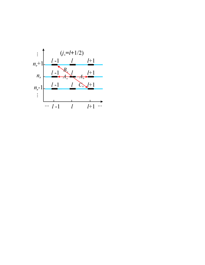
Figure 2: The algebra structure of the 3D Landau levels in the positive helicity sector. Operators $A_{\pm}(l)$ connect states with different $l$ in the same Landau level, while $B_{-}(l)$ and $C_{+}(l)$ connect those between neighboring Landau levels.

Appendix A The ladder algebra for the spectra flatness

The degeneracy of the 3D LL over different values of angular momentum is not accidental, but protected by a ladder algebra constructed below. For example, we take the case of $qG>0$ and consider the positive helicity Landau level states of $H_{+}$. The variable transformation for the radial eigenstates is applied as $\chi_{n_{r},l}(r)=rR_{n_{r},l}(r)$, and the corresponding radial Hamiltonians become

$$H_{l}=\hbar\omega_{0}\Big{\{}-\frac{d^{2}}{dr^{\ast 2}}+\frac{l(l+1)}{r^{\ast 2}}-l+\frac{1}{4}r^{\ast 2}\Big{\}},$$ (10)

where the dimensionless radius is $r^{\ast}=\frac{r}{l_{G}}$. The ladder operators are defined as

$$A_{+}(l) = \frac{d}{dr^{\ast}}-\frac{l+1}{r^{\ast}}-\frac{1}{2}r^{\ast},$$

$$A_{-}(l) = -\frac{d}{dr^{\ast}}-\frac{l}{r^{\ast}}-\frac{1}{2}r^{\ast}.$$ (11)

They satisfy the relations

$$H_{l\pm 1}A_{\pm}(l)=A_{\pm}(l)H_{l}.$$ (12)

Consequentially, $\chi_{n_{r},l\pm 1}=A_{\pm}(l)\chi_{n_{r},l}$ with the same energy independent of $l$. All the states in the same LL can be reached by successively applying $A_{\pm}$ operators.

To connect different LLs, other two ladder operators are defined as

$$B_{-}(l) = -\frac{d}{dr^{\ast}}-\frac{l}{r^{\ast}}+\frac{1}{2}r^{\ast},$$

$$C_{+}(l) = \frac{d}{dr^{\ast}}-\frac{l+1}{r^{\ast}}+\frac{1}{2}r^{\ast},$$ (13)

which satisfy

$$H_{l-1}B_{-}(l) = B_{-}(l)(H_{l}+2\hbar\omega_{0}),$$

$$H_{l+1}C_{+}(l) = C_{+}(l)(H_{l}-2\hbar\omega_{0}),$$ (14)

respectively. By applying $B_{-}(l)$ ($C_{+}(l)$) to $\chi_{n_{r},l}(r)$, we arrive at

$$\chi_{n_{r}+1,l-1} = B_{-}(l)\chi_{n_{r},l},$$

$$\chi_{n_{r}-1,l+1} = C_{+}(l)\chi_{n_{r},l},$$ (15)

where the energy shifts $\pm 2\hbar\omega_{0}$, respectively, as illustrated in Fig. 2. Similar algebra can also be constructed for the case of $qG<0$.

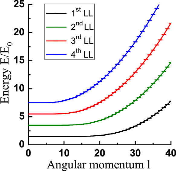
Figure 3: The energy dispersion of the first four Landau levels v.s. $l=j-\frac{1}{2}$. Open boundary condition is used for a ball with the radius $R_{0}/l_{G}=8$. The edge states correspond to those with large values of $l$ and develop linear dispersions with $l$. The most probable radius of the LLL state with $l$ is $r=l_{G}\sqrt{l}$.

Appendix B Numerical calculation for the gapless surface Dirac modes

The surface states of the 3D LL Hamiltonian Eq. 2 in the main text are gapless helical Dirac modes. We have numerically calculated the spectra with the open boundary condition for the positive helicity states with $j_{+}=l+\frac{1}{2}$. The results for the first four LLs are plotted in Fig. 3. For the lowest LL (LLL) states, when the orbital angular momentum $l$ exceeds a characteristic value $l_{c}\approx 30$, the spectra become dispersive indicating the onset of surface states. Although the surface spectra look very similar to those of the 2D quantum Hall edges, a crucial difference is that each $l$ in Fig. 3 does not represent a single chiral state but a set of helical states of $2j_{+}+1$ fold degeneracy with $j_{+}=l+\frac{1}{2}$.

Appendix C Quaternionic wavefunction for the $j_{-}$ sector  

In the main text, we have showed that the 3D LLL states with the positive helicity in the quaternion representation form a set of complete basis for the quaternionic left-analytic polynomials. For the case of the LLL with negative helicity, their quaternionic version $g^{LLL}_{j_{-},j_{z}}(x,y,z)$ are not analytic any more. Nevertheless, since the wavefunctions of the negative helicity sector can be related to the positive one via $\mathcal{Y}_{j_{-},j_{z};l+1}(\hat{\Omega})=-\vec{\sigma}\cdot\hat{\Omega}\mathcal{Y}_{j_{+},j_{z};l}(\hat{\Omega})$, where $\vec{\sigma}\cdot\hat{\Omega}$ has odd parity, their quaternionic version is related to the analytic one through $g^{LLL}_{j_{-}=(l+1)-\frac{1}{2},j_{z}}=(-\hat{x}k-\hat{y}j+\hat{z}i)f^{LLL}_{j_{+}=l+\frac{1}{2},j_{z}}i$. Here, the representation of quaternion imaginary units $\{i,j,k\}$ as Pauli matrices $\{i\sigma_{z},-i\sigma_{y},-i\sigma_{x}\}$ are used, as derived from the rotational properties of the spin-orbit coupled spheric harmonics.

Appendix D Generalization to $N$-dimensions

The study in 3D and 4D LL systems can be generalized to $N$-D by replacing the vector and scalar potentials in Eq. 1 in the main text with the $SO(N)$ gauge field

$$A^{a}(\vec{r})=gr^{b}S^{ab},\ \ \,V(r)=-\frac{N-2}{2}m\omega_{0}r^{2},$$ (16)

respectively, where $S^{ab}$ are the $SO(N)$ spin operators constructed based on the Clifford algebra. The rank-$k$ Clifford algebra contains $2k+1$ matrices with the dimension $2^{k}\times 2^{k}$ which anti-commute with each other denoted as $\Gamma^{a}~{}(1\leq a\leq 2k+1)$. Their commutators generate

$$\Gamma^{ab}=-\frac{i}{2}[\Gamma^{a},\Gamma^{b}],$$ (17)

for $1\leq a<b\leq 2k+1$. For odd dimensions $N=2k+1$, the $SO(N)$ spin operators in the fundamental spinor representation can be constructed by using the rank-$k$ matrices as $S^{ab}=\frac{1}{2}\Gamma^{ab}$. For even dimensions $N=2k+2$, we can select $2k+2$ ones among the $2k+3$ $\Gamma$-matrices of rank-$(k+1)$ to form $S^{ab}=\frac{1}{2}\Gamma^{ab}$, then all of $S^{ab}$ commute with $\Gamma^{2k+3}$. This $2^{k+1}$-D spinor representation of $S^{ab}$ is thus reducible into the fundamental and anti-fundamental representations. Both of them are $2^{k}$-D, which can be constructed from the rank-$k$ $\Gamma$-matrices as $S^{a,2k+2}=\pm\frac{1}{2}\Gamma^{a}(1\leq a\leq 2k+1)$ and $S^{ab}=\frac{1}{2}\Gamma^{ab}(1\leq a<b<2k+1)$, respectively.

As for TR properties, $\Gamma^{a}$’s are TR even and odd at even and odd values of $k$, respectively. We conclude that at $N=2k+1$, the $N$-D version of the LL Hamiltonian is TR invariant in the fundamental spinor representation. At $N=4k$, it is also TR invariant in both the fundamental and anti-fundamental representations. However $N=4k+2$, each one of the fundamental and anti-fundamental representations is not TR invariant, but transforms into each other under TR operation.

Similarly, the $N$-D LL Hamiltonian can be reorganized as the harmonic oscillator with SO coupling. For the case of $qG>0$, it becomes

$$H_{N,+}=\frac{p^{2}}{2m}+\frac{1}{2}m\omega_{0}^{2}r^{2}-\hbar\omega_{0}\Gamma_{ab}L_{ab},$$ (18)

where $L_{ab}=r_{a}p_{b}-r_{b}p_{a}$ with $1\leq a<b\leq N$. The $l$-th order $N$-D spherical harmonic functions are eigenstates of $L^{2}=L_{ab}L_{ab}$ with the eigenvalue of $\hbar^{2}l(l+D-2)$. The $N$-$D$ harmonic oscillator has the energy spectra of $E_{n_{r},l}=(2n_{r}+l+N/2)\hbar\omega$. When coupling to the fundamental spinors, the $l$-th spherical harmonics split into the positive helicity ($j_{+}$) and negative helicity $(j_{-})$ sectors, whose eigenvalues of the $\Gamma_{ab}L_{ab}$ are $\hbar l$ and $-\hbar(l+N-2)$, respectively. For the positive helicity sector, its spectra become independent of $l$ as $E_{+}=(2n_{r}+N/2)\hbar\omega$, with the radial wave functions are

$$R_{n_{r}l}(r)=r^{l}e^{-r^{2}/4l_{G}^{2}}F(-n_{r},l+N/2,r^{2}/2l_{G}^{2}).$$ (19)

The highest weight states in the LLL can be written as

$$\psi_{ab,\pm l}^{hw}(\vec{r})=[(\hat{e}_{a}\pm i\hat{e}_{b})\cdot\vec{r}]^{l}e^{-r^{2}/4l_{G}^{2}}\otimes\alpha_{\pm,ab},$$ (20)

where $\alpha_{\pm,ab}$ is the eigenstate of $\Gamma_{ab}$ with eigenvalue $\pm 1$, respectively. The magnetic translation in the $ab$-plane by the displacement vector $\vec{\delta}$ takes the form

$$T_{ab}(\vec{\delta})=\exp\big{[}-\vec{\delta}\cdot\vec{\nabla}+\frac{i}{2l_{G}^{2}}\Gamma_{ab}(r_{a}\delta_{b}-r_{b}\delta_{a})\big{]}.$$ (21)

Similarly to the 3D case, staring from the LLL state localized around the origin with $l=0$, we can perform the magnetic translation and Fourier transformation with respect to the transverse spin polarization. The resultant localized Gaussian pockets are LLL states of the eigenstates of the $SO(N-1)$ symmetry with respect to the translation direction $\vec{\delta}$. Again each LL contributes to one channel of surface Dirac modes on $S^{N-1}$ described by $H_{bd}=(v_{f}/R_{0})\Gamma_{ab}L_{ab}-\mu$.

References

- (1) K. Klitzing, G. Dorda, and M. Pepper, Phys. Rev. Lett. 45, 494 (1980).
- (2) D. C. Tsui, H. L. Stormer, and A. C. Gossard, Phys. Rev. Lett. 48, 1559 (1982).
- (3) D. J. Thouless, M. Kohmoto, M. P. Nightingale, and M. den Nijs, Phys. Rev. Lett. 49, 405 (1982).
- (4) F. D. M. Haldane, Phys. Rev. Lett. 61, 2015 (1988).
- (5) J. E. Avron, R. Seiler, and B. Simon, Phys. Rev. Lett. 51, 51 (1983).
- (6) Q. Niu, D. Thouless, and Y. Wu, Phys. Rev. B 31, 3372 (1985).
- (7) M. Kohmoto, Ann. Phys. 160, 343 (1985).
- (8) J. E. Avron, R. Seiler, and B. Simon, Phys. Rev. Lett. 65, 2185 (1990).
- (9) R. Laughlin, Phys. Rev. B 23, 5632 (1981).
- (10) B. I. Halperin, Phys. Rev. B 25, 2185 (1982).
- (11) B. A. Bernevig and S. C. Zhang, Phys. Rev. Lett. 96, 106802 (2006).
- (12) C. L. Kane and E. J. Mele, Phys. Rev. Lett. 95, 146802 (2005).
- (13) C. L. Kane and E. J. Mele, Phys. Rev. Lett. 95, 226801 (2005).
- (14) L. Fu and C. L. Kane, Phys. Rev. B 76, 045302 (2007).
- (15) L. Fu, C. L. Kane, and E. J. Mele, Phys. Rev. Lett. 98, 106803 (2007).
- (16) J. E. Moore and L. Balents, Phys. Rev. B 75, 121306 (2007).
- (17) B. A. Bernevig, T. L. Hughes, and S. C. Zhang, Science 314, 1757 (2006).
- (18) X. L. Qi, T. L. Hughes, and S. C. Zhang, Phys. Rev. B 78, 195424 (2008).
- (19) R. Roy, Phys. Rev. B 79, 195322 (2009).
- (20) R. Roy, New J. Phys. 12, 065009 (2010).
- (21) M. Z. Hasan and C. L. Kane, Rev. Mod. Phys. 82, 3045 (2010).
- (22) X. L. Qi and S. C. Zhang, Rev. Mod. Phys. 83, 1057 (2011).
- (23) M. König et al., Science 318, 766 (2007).
- (24) D.-X. Qu et al., Science 329, 821 (2010).
- (25) J. Xiong et al., Physica E 44, 917 (2012).
- (26) P. Roushan et al., Nature 460, 1106 (2009).
- (27) D. Hsieh et al., Nature 452, 970 (2008).
- (28) D. Hsieh et al., Phys. Rev. Lett. 103, 146401 (2009).
- (29) Y. Xia et al., Nature Phys. 5, 398 (2009).
- (30) Y. Chen et al., Science 325, 178 (2009).
- (31) Z. Alpichshev et al., Phys. Rev. Lett. 104, 16401 (2010).
- (32) T. Zhang et al., Phys. Rev. Lett. 103, 266803 (2009).
- (33) R. Laughlin, Phys. Rev. Lett. 50, 1395 (1983).
- (34) F. Haldane, Phys. Rev. Lett. 51, 605 (1983).
- (35) B. I. Halperin, Phys. Rev. Lett. 52, 1583 (1984).
- (36) S. Girvin and T. Jach, Phys. Rev. B 29, 5617 (1984).
- (37) D. Arovas, J. R. Schrieffer, and F. Wilczek, Phys. Rev. Lett. 53, 722 (1984).
- (38) F. D. M. Haldane and E. H. Rezayi, Phys. Rev. Lett. 54, 237 (1985).
- (39) S. Girvin and A. MacDonald, Phys. Rev. Lett. 58, 1252 (1987).
- (40) J. K. Jain, Phys. Rev. Lett. 63, 199 (1989).
- (41) J. K. Jain, Composite fermions (Cambridge University Press, 2007).
- (42) S. C. Zhang, T. H. Hansson, and S. Kivelson, Phys. Rev. Lett. 62, 82 (1989).
- (43) G. Moore and N. Read, Nucl. Phys. B 360, 362 (1991).
- (44) X.-G. Wen, Int. J. Mod. Phys. B 06, 1711 (1992).
- (45) S. Sondhi, A. Karlhede, S. Kivelson, and E. Rezayi, Phys. Rev. B 47, 16419 (1993).
- (46) G. Murthy and R. Shankar, Rev. Mod. Phys. 75, 1101 (2003).
- (47) S. Das Sarma, M. Freedman, and C. Nayak, Phys. Rev. Lett. 94, 166802 (2005).
- (48) S. Das Sarma and A. Pinczuk, Perspectives in quantum Hall effects (Wiley-VCH, 2008).
- (49) S. C. Zhang and J. P. Hu, Science 294, 823 (2001).
- (50) B. A. Bernevig et al., Ann. Phys. 300, 185 (2002).
- (51) H. Elvang and J. Polchinski, Comptes Rendus Physique 4, 405 (2003).
- (52) M. Fabinger, J. High Energy Phys. 05 (2002) 037 (2002).
- (53) B. A. Bernevig, J. Hu, N. Toumbas, and S. C. Zhang, Phys. Rev. Lett. 91, 236803 (2003).
- (54) K. Hasebe, Symmetry, Integrability and Geometry: Methods and Applications 6, 071 (2010).
- (55) B. Bagchi, Supersymmetry in quantum and classical mechanics (Chapman & Hall/CRC, 2001).
- (56) J. E. Hirsch, Europhys. Lett. 81, 67003 (2008).
- (57) J. E. Hirsch, Annalen der Physik 17, 380 (2008).
- (58) J. E. Hirsch, (private communication); Journal of Superconductivity and Novel Magnetism 26, 2239 (2013)..
- (59) A. V. Balatsky, arXiv:cond-mat/9205006 (1992).
- (60) S. Adler, Quaternionic quantum mechanics and quantum fields (Oxford University Press, USA, 1995), Vol. 88.
- (61) Y. Li, X. Zhou, and C. Wu, arXiv:1205.2162 (2012).
- (62) A. Sudbery, Math. Proc. Cambridge Philos. Soc 85, 199 (1979).
- (63) See Supplemental Material at the appendix for discussions on the ladder algebra generating 3D LL states, quaternionic properties of 3D LL wave functions in the negative helicity branch, the surface spectra and generalizations to arbitrary higher dimensional flat space.
- (64) N. Gemelke, E. Sarajlic, and S. Chu, arXiv preprint arXiv:1007.2677 (2010).
- (65) Y. J. Lin, K. Jiménez-García, and I. B. Spielman, Nature 471, 83 (2011).
- (66) J. Dalibard, F. Gerbier, G. Juzeliūnas, and P. Öhberg, Rev. Mod. Phys. 83, 1523 (2011).
- (67) X. Zhou, Y. Li, and C. Wu, in preparation .
- (68) S. C. Zhang, private communication .
Supplemental Material for “Topological insulators with quaternionic analytic Landau levels”