Networked Controller Design using Packet Delivery Prediction in Mesh Networks

Abstract

Much of the current theory of networked control systems uses simple point-to-point communication models as an abstraction of the underlying network. As a result, the controller has very limited information on the network conditions and performs suboptimally. This work models the underlying wireless multihop mesh network as a graph of links with transmission success probabilities, and uses a recursive Bayesian estimator to provide packet delivery predictions to the controller. The predictions are a joint probability distribution on future packet delivery sequences, and thus capture correlations between successive packet deliveries. We look at finite horizon LQG control over a lossy actuation channel and a perfect sensing channel, both without delay, to study how the controller can compensate for predicted network outages.

Network Estimation and Packet Delivery Prediction for Control over Wireless Mesh Networks The work was supported by the EU project FeedNetBack, the Swedish Research Council, the Swedish Strategic Research Foundation, the Swedish Governmental Agency for Innovation Systems, and the Knut and Alice Wallenberg Foundation. PHOEBUS CHEN, CHITHRUPA RAMESH, AND KARL H. JOHANSSON Stockholm 2010   ACCESS Linnaeus Centre Automatic Control School of Electrical Engineering KTH Royal Institute of Technology SE-100 44 Stockholm, Sweden TRITA-EE:043

1 Introduction

Increasingly, control systems are operated over large-scale, networked infrastructures. In fact, several companies today are introducing devices that communicate over low-power wireless mesh networks for industrial automation and process control [1, 2]. While wireless mesh networks can connect control processes that are physically spread out over a large space to save wiring costs, these networks are difficult to design, provision, and manage [3, 4]. Furthermore, wireless communication is inherently unreliable, introducing packet losses and delays, which are detrimental to control system performance and stability.

Research in the area of Networked Control Systems (NCSs) [5] addresses how to design control systems which can account for the lossy, delayed communication channels introduced by a network. Traditional tasks in control systems design, like stability/performance analysis and controller/estimator synthesis, are revisited, with network models providing statistics about packet losses and delays. In the process, the studies highlight the benefits and drawbacks of different system architectures. For example, Figure 1 depicts the general system architecture of a networked control system over a mesh network proposed by Robinson and Kumar [6]. A fundamental architecture problem is how to choose the best location to place the controllers, if they can be placed at any of the sensors, actuators, or communication relay nodes in the network. One insight from Schenato et al. [7] is that if the controller can know whether the control packet reaches the actuator, e.g., we place the controller at the actuator, then the optimal LQG controller and estimator can be designed separately (the separation principle).

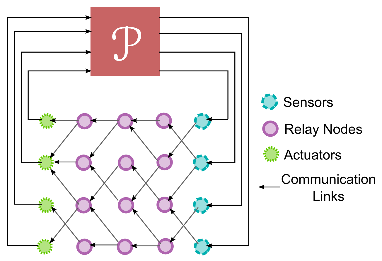
Figure 1: A networked control system over a mesh network, where the controllers can be located on any node.

To gain more insights on how to architect and design NCSs, two limitations in the approach of many current NCS research studies need to be addressed. The first limitation is the use of simple models of packet delivery over a point-to-point link or a star network topology to represent the network, which are often multihop and more complex. The second limitation is the treatment of the network as something designed and fixed a priori before the design of the control system. Very little information is passed through the interface between the network and the control system, limiting the interaction between the two “layers” to tune the controller to the network conditions, and vice versa.

1.1 Related Works

Schenato et al. [7] and Ishii [8] study stability and controller synthesis for different control system architectures, but they both model networks as i.i.d. Bernoulli processes that drop packets on a single link. The information passed through the interface between the network and the control system is the packet drop probability of the link, which is assumed to be known and fixed. Seiler and Sengupta [9] study stability and $\mathcal{H}_{\infty}$ controller synthesis when the network is modeled as a packet-dropping link described by a two-state Markov chain (Gilbert-Elliott model), where the information passed through the network-controller interface are the transition probabilities of the Markov chain. Elia [10] studies stability and the synthesis of a stabilizing controller when the network is represented by an LTI system with stochastic disturbances modeled as parallel, independent, multiplicative fading channels.

Some related work in NCSs do use models of multihop networks. For instance, work on consensus of multi-agent systems [11] typically study how the connectivity graph(s) provided by the network affects the convergence of the system, and is not focused on modeling the links. Robinson and Kumar [6] study the optimal placement of a controller in a multihop network with i.i.d. Bernoulli packet-dropping links, where the packet drop probability is known to the controller. Gupta et al. [12] study how to optimally process and forward sensor measurements at each node in a multihop network for optimal LQG control, and analyze stability when packet drops on the links are modeled as spatially-independent Bernoulli, spatially-independent Gilbert-Elliott, or memoryless spatially-correlated processes. Varagnolo et al. [13] compare the performance of a time-varying Kalman filter on a wireless TDMA mesh network under unicast routing and constrained flooding. The network model describes the routing topology and schedule of an implemented communication protocol, TSMP [14], but it assumes that transmission successes on the links are spatially-independent and memoryless. Both Gupta et al. [12] and Varagnolo et al. [13] are concerned with estimation when packet drops occur on the sensing channel, and the estimators do not need to know network parameters like the packet loss probability.

1.2 Contributions

Our approach is a step toward using more sophisticated, multihop network models and passing more information through the interface between the controller and the network. Similar to Gupta et al. [12], we model the network routing topology as a graph of independent links, where transmission success on each link is described by a two-state Markov chain. The network model consists of the routing topology and a global TDMA transmission schedule. Such a minimalist network model captures the essence of how a network with bursty links can have correlated packet deliveries [15], which are particularly bad for control when they result in bursts of packet losses. Using this model, we propose a network estimator to estimate, without loss of information, the state of the network given the past packet deliveries. The network estimate is translated to a joint probability distribution predicting the success of future packet deliveries, which is passed through the network-controller interface so the controller can compensate for unavoidable network outages. The network estimator can also be used to notify a network manager when the network is broken and needs to be reconfigured or reprovisioned, a direction for future research.

Section 2 describes our plant and network models. We propose two network estimators, the Static Independent links, Hop-by-hop routing, Scheduled (SIHS) network estimator and the Gilbert-Elliott Independent links, Hop-by-hop routing, Scheduled (GEIHS) network estimator in Section 3. Next, we design a finite-horizon, Future-Packet-Delivery-optimized (FPD) LQG controller to utilize the packet delivery predictions provided by the network estimators, presented in Section 4. Section 5 provides an example and simulations demonstrating how the GEIHS network estimator combined with the FPD controller can provide better performance than a classical LQG controller or a controller assuming i.i.d. packet deliveries. Finally, Section 7 describes the limitations of our approach and future work.

2 Problem Formulation

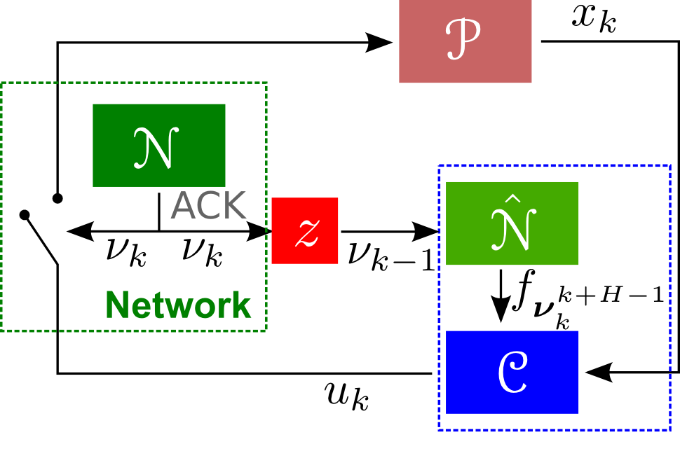
Figure 2: A control loop for plant ${\mathscr{P}}$ with the network on the actuation channel. The network estimator $\hat{{\mathscr{N}}}$ passes packet delivery predictions $f_{\bm{\nu}_{{}^{k}}^{{}_{k+H-1}}}$ to the FPD controller ${\mathscr{C}}$, with past packet delivery information obtained from the network ${\mathscr{N}}$ over an acknowledgement (ACK) channel.

This paper studies an instance of the general system architecture depicted in Figure 1, with a single control loop containing one sensor and one actuator. One network estimator and one controller are placed at the sensor, and we assume that an end-to-end acknowledgement (ACK) that the controller-to-actuator packet is delivered is always received at the network estimator, as shown in Figure 2. For simplicity, we assume that the plant dynamics are significantly slower than the end-to-end packet delivery deadline, so that we can ignore the delay introduced by the network. The general problem is to jointly design a network estimator and controller that can optimally control the plant using our proposed SIHS and GEIHS network models. In our problem setup, the controller is only concerned with the past, present, and future packet delivery sequence and not with the detailed behavior of the network, nor can it affect the behavior of the network. Therefore, the network estimation problem decouples from the control problem. The information passed through the network-controller interface is the packet delivery sequence, specifically the joint probability distribution describing the future packet delivery predictions.

2.1 Plant and Network Models

The state dynamics of the plant ${\mathscr{P}}$ in Figure 2 is given by

$$x_{k+1}=Ax_{k}+\nu_{k}Bu_{k}+w_{k}\quad,$$ (1)

where $A\in{\mathbb{R}}^{\ell\times\ell}$, $B\in{\mathbb{R}}^{\ell\times m}$, and $w_{k}$ are i.i.d. zero-mean Gaussian random variables with covariance matrix $R_{w}\in{\mathbb{S}}_{+}^{\ell}$, where ${\mathbb{S}}_{+}^{\ell}$ is the set of $\ell\times\ell$ positive semidefinite matrices. The initial state $x_{0}$ is a zero-mean Gaussian random variable with covariance matrix $R_{0}\in{\mathbb{S}}_{+}^{\ell}$ and is mutually independent of $w_{k}$. The binary random variable $\nu_{k}$ indicates whether a packet from the controller reaches the actuator ($\nu_{k}=1$) or not ($\nu_{k}=0$), and each $\nu_{k}$ is independent of $x_{0}$ and $w_{k}$ (but the $\nu_{k}$’s are not independent of each other).

Let the discrete sampling times for the control system be indexed by $k$, but let the discrete time for schedule time slots (described below) be indexed by $t$. The time slot intervals are smaller than the sampling intervals. The time slot when the control packet at sample time $k$ is generated is denoted $t_{k}$, and the deadline for receiving the control packet at the receiver is $t_{k}^{\prime}$. We assume that $t_{k}^{\prime}\leq t_{k+1}$ for all $k$. Figure 3 illustrates the relationship between $t$ and $k$.

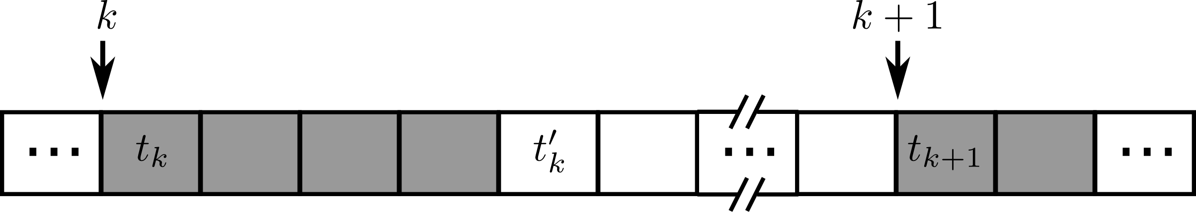
Figure 3: The packet containing the control input $u_{k}$ is generated right before time slot $t_{k}$. The packet may be in transit through the network in the shaded time slots, until right before time slot $t_{k}^{\prime}$. Thus, time $t_{k}$ is aligned with the beginning of the time slot.

The model of the TDMA wireless mesh network (${\mathscr{N}}$ in Figure 2) consists of a routing topology $G$, a link model describing how the transmission success of a link evolves over time, and a fixed repeating schedule $\mathbf{F}^{(T)}$. The SIHS network model and the GEIHS network model only differ in the link model. Each of these components will be described in detail below.

The routing topology is described by $G=({\mathcal{V}},{\mathcal{E}})$, a connected directed acyclic graph with the set of vertices (nodes) ${\mathcal{V}}=\{1,\dots,M\}$ and the set of directed edges (links) ${\mathcal{E}}\subseteq\{(i,j)\>:\>i,j\in{\mathcal{V}},\>i\neq j\}$, where the number of edges is denoted $E$. The source node is denoted $a$ and the sink (destination) node is denoted $b$. Only the destination node has no outgoing edges.

At any moment in time, the links in $G$ can be either be up (succeeds if attempt to transmit packet) or down (fails if attempt to transmit packet). Thus, there are $2^{E}$ possible topology realizations $\tilde{G}=({\mathcal{V}},\tilde{{\mathcal{E}}})$, where $\tilde{{\mathcal{E}}}\subseteq{\mathcal{E}}$ represents the edges that are up.

At time $t_{k}$, the actual state of the topology is one of the topology realizations but it is not known to the network estimator. With some abuse of terminology, we define $G^{{}_{(k)}}$ to be the random variable representing the state of the topology at time $t_{k}$.

This paper considers the network under two link models, the static link model and the Gilbert-Elliott (G-E) link model. Both network models assume all the links in the network are independent.

The static link model assumes the links do not switch between being up and down while packets are sent through the network. Therefore, the sequence of topology realizations over time is constant. While not realistic, it leads to the simple network estimator in Section 3.1 for pedagogical purposes. The a priori transmission success probability of link $l=(i,j)$ is $p_{l}$.

The G-E link model represents each link $l$ by the two-state Markov chain shown in Figure 4. At each sample time $k$, a link in state 0 (down) transitions to state 1 (up) with probability $p_{l}^{\mathrm{u}}$, and a link from state 1 transitions to state 0 with probability $p_{l}^{\mathrm{d}}$. The steady-state probability of being in state 1, which we use as the a priori probability of the link being up, is

$$p_{l}=p_{l}^{\mathrm{u}}/(p_{l}^{\mathrm{u}}+p_{l}^{\mathrm{d}})\quad.$$

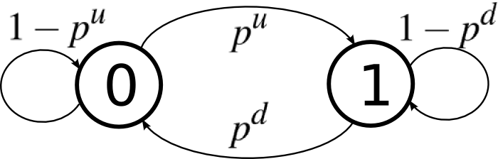
Figure 4: Gilbert-Elliott link model

The fixed, repeating schedule of length $T$ is represented by a sequence of matrices $\mathbf{F}^{(T)}=(F^{(1)},F^{(2)},\dots,F^{(T)})$, where the matrix $F^{(t-1\pmod{T}+1)}$ represents the links scheduled at time $t$. The matrix $F^{(t)}\in\{0,1\}^{M\times M}$ is defined from the set ${\mathcal{F}}^{(t)}\subseteq{\mathcal{E}}$ containing the links scheduled for transmission at time $t$. We assume that nodes can only unicast packets, meaning that for all nodes $i$, if $(i,j)\in{\mathcal{F}}^{(t)}$ then for all $v\neq j,(i,v)\not\in{\mathcal{F}}^{(t)}$. Furthermore, a node holds onto a packet if the transmission fails and can retransmit the packet the next time an outgoing link is scheduled (hop-by-hop routing). Thus, the matrix $F^{(t)}$ has entries

$$F_{ij}^{(t)}=\begin{cases}1&\text{if $(i,j)\in{\mathcal{F}}^{(t)}$, or}\\ &\text{if $i=j$ and $\forall v\in{\mathcal{V}},(i,v)\not\in{\mathcal{F}}^{(t)}$}\\ 0&\text{otherwise.}\end{cases}$$

An exact description of the network consists of the sequence of topology realizations over time and the schedule $\mathbf{F}^{(T)}$. Assuming a topology realization $\tilde{G}$, the links that are scheduled and up at any given time $t$ are represented by the matrix $\tilde{F}^{(t;\tilde{G})}\in\{0,1\}^{M\times M}$, with entries

$$\tilde{F}_{ij}^{(t;\tilde{G})}=\begin{cases}1&\text{if $(i,j)\in{\mathcal{F}}^{(t)}\cap\tilde{{\mathcal{E}}}$, or }\\ &\text{if $i=j$ and $\forall v\in{\mathcal{V}},(i,v)\not\in{\mathcal{F}}^{(t)}\cap\tilde{{\mathcal{E}}}$}\\ 0&\text{otherwise.}\end{cases}$$ (2)

Define the matrix $\tilde{F}^{(t,t^{\prime};\tilde{G})}=\tilde{F}^{(t;\tilde{G})}\tilde{F}^{(t+1;\tilde{G})}\dotsm\tilde{F}^{(t^{\prime};\tilde{G})}$, such that entry $\tilde{F}_{ij}^{(t,t^{\prime};\tilde{G})}$ is 1 if a packet at node $i$ at time $t$ will be at node $j$ at time $t^{\prime}$, and is 0 otherwise. Since the destination $b$ has no outgoing links, a packet sent from the source $a$ at time $t$ reaches the destination $b$ at or before time $t^{\prime}$ if and only if $\tilde{F}_{ab}^{(t,t^{\prime};\tilde{G})}=1$. To simplify the notation, let the function $\delta_{\kappa}$ indicate whether the packet delivery $\tilde{\nu}\in\{0,1\}$ is consistent with the topology realization $\tilde{G}$, assuming the packet was generated at $t_{\kappa}$, i.e.,

$$\delta_{\kappa}(\tilde{\nu};\tilde{G})=\begin{cases}1&\text{if $\tilde{\nu}=\tilde{F}_{ab}^{(t_{\kappa},t_{\kappa}^{\prime};\tilde{G})}$}\\ 0&\text{otherwise.}\end{cases}$$ (3)

The function assumes the fixed repeating schedule $\mathbf{F}^{(T)}$, the packet generation time $t_{\kappa}$, the deadline $t_{\kappa}^{\prime}$, the source $a$, and the destination $b$ are implicitly known.

2.2 Network Estimators

As shown in Figure 2, at each sample time $k$ the network estimator $\hat{{\mathscr{N}}}$ takes as input the previous packet delivery $\nu_{k-1}$, estimates the topology realization using the network model and all past packet deliveries, and outputs the joint probability distribution of future packet deliveries $f_{\bm{\nu}_{{}^{k}}^{{}_{k+H-1}}}$. For clarity in the following exposition, let ${\mathscr{V}}_{\kappa}\in\{0,1\}$ be the value taken on by the packet delivery random variable $\nu_{\kappa}$ at some past sample time $\kappa$. Let the vector $\bm{{\mathscr{V}}}_{{}^{0}}^{{}_{k-1}}=[{\mathscr{V}}_{0},\dots,{\mathscr{V}}_{k-1}]$ denote the history of packet deliveries at sample time $k$, the values taken on by the vector of random variables $\bm{\nu}_{{}^{0}}^{{}_{k-1}}=[\nu_{0},\dots,\nu_{k-1}]$. Then,

$$f_{\bm{\nu}_{{}^{k}}^{{}_{k+H-1}}}(\bm{\tilde{\nu}}_{{}^{0}}^{{}_{H-1}})=\operatorname{{\mathbb{P}}}(\bm{\nu}_{{}^{k}}^{{}_{k+H-1}}=\bm{\tilde{\nu}}_{{}^{0}}^{{}_{H-1}}|\bm{\nu}_{{}^{0}}^{{}_{k-1}}=\bm{{\mathscr{V}}}_{{}^{0}}^{{}_{k-1}})$$ (4)

is the prediction of the next $H$ packet deliveries, where $\bm{\nu}_{{}^{k}}^{{}_{k+H-1}}=[\nu_{k},\dots,\nu_{k+H-1}]$ is a vector of random variables representing future packet deliveries and $\bm{\tilde{\nu}}_{{}^{0}}^{{}_{H-1}}\in\{0,1\}^{H}$.

The SIHS and GEIHS network estimators only differ in the network models. The parameters of the network models — topology $G$, schedule $\mathbf{F}^{(T)}$, link probabilities $\{p_{l}\}_{l\in{\mathcal{E}}}$ or $\{p_{l}^{\mathrm{u}},p_{l}^{\mathrm{d}}\}_{l\in{\mathcal{E}}}$, source $a$, sink $b$, packet generation times $t_{k}$, and deadlines $t_{k}^{\prime}$ — are known a priori to the network estimators and are left out of the conditional probability expressions.

In Section 3, we will use the probability distribution on the topology realizations (our network state estimate),

$$\operatorname{{\mathbb{P}}}(G^{{}_{(k)}}=\tilde{G}|\bm{\nu}_{{}^{0}}^{{}_{k-1}}=\bm{{\mathscr{V}}}_{{}^{0}}^{{}_{k-1}})\quad,$$

to obtain $f_{\bm{\nu}_{{}^{k}}^{{}_{k+H-1}}}$ from $\bm{{\mathscr{V}}}_{{}^{0}}^{{}_{k-1}}$ and the network model.

2.3 FPD Controller

The FPD controller (${\mathscr{C}}$ in Figure 2) optimizes the control signals to the statistics of the future packet delivery sequence, derived from the past packet delivery sequence. We choose the optimal control framework because the cost function allows us to easily compare the FPD controller with other controllers. The control policy operates on the information set

$${\mathcal{I}}^{{}^{\mathscr{C}}}_{k}=\{\bm{x}_{{}^{0}}^{{}_{k}},\bm{u}_{{}^{0}}^{{}_{k-1}},\bm{\nu}_{{}^{0}}^{{}_{k-1}}\}\quad.$$ (5)

The control policy minimizes the linear quadratic cost function

$$\operatorname*{{\mathbb{E}}}\left[\scriptstyle x_{N}^{T}Q_{0}x_{N}+\sum_{n=0}^{N-1}x_{n}^{T}Q_{1}x_{n}+\nu_{n}u_{n}^{T}Q_{2}u_{n}\displaystyle\right]\quad,$$ (6)

where $Q_{0}$, $Q_{1}$, and $Q_{2}$ are positive definite weighting matrices and $N$ is the finite horizon, to get the minimum cost

$$J=\min_{{}_{u_{0},\dots,u_{N-1}}}\operatorname*{{\mathbb{E}}}\left[\scriptstyle x_{N}^{T}Q_{0}x_{N}+\sum_{n=0}^{N-1}x_{n}^{T}Q_{1}x_{n}+\nu_{n}u_{n}^{T}Q_{2}u_{n}\displaystyle\right]\quad.$$

Section 4 will show that the resulting architecture separates into a network estimator and a controller which uses the pdf $f_{\bm{\nu}_{{}^{k}}^{{}_{k+H-1}}}$ supplied by the network estimator ($\hat{{\mathscr{N}}}$ in Figure 2) to find the control signals $u_{k}$.

3 Network Estimation and Packet Delivery Prediction

We will use recursive Bayesian estimation to estimate the state of the network, and use the network state estimate to predict future packet deliveries. Figure 5 is the graphical model / hidden Markov model [16] describing our recursive estimation problem.

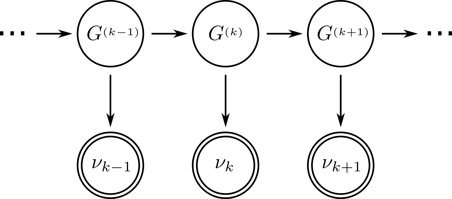
Figure 5: Graphical model describing the network estimation problem. $\nu_{k}$ is the measurement output variable at time $k$, and $G^{{}_{(k)}}$ is the hidden state of the network.

3.1 SIHS Network Estimator

The steps in the SIHS network estimator are derived from (4). We introduce new notation for conditional pdfs (i.e., $\alpha_{k},\beta_{k},Z_{k}$), which will be used later to state the steps in the estimator compactly. First, express $f_{\bm{\nu}_{{}^{k}}^{{}_{k+H-1}}}(\bm{\tilde{\nu}}_{{}^{0}}^{{}_{H-1}})$ as

$$\underbrace{\operatorname{{\mathbb{P}}}(\bm{\nu}_{{}^{k}}^{{}_{k+H-1}}=\bm{\tilde{\nu}}_{{}^{0}}^{{}_{H-1}}|\bm{\nu}_{{}^{0}}^{{}_{k-1}}=\bm{{\mathscr{V}}}_{{}^{0}}^{{}_{k-1}})}_{f_{\bm{\nu}_{{}^{k}}^{{}_{k+H-1}}}(\bm{\tilde{\nu}}_{{}^{0}}^{{}_{H-1}})}=\sum_{\tilde{G}}\underbrace{\operatorname{{\mathbb{P}}}(\bm{\nu}_{{}^{k}}^{{}_{k+H-1}}=\bm{\tilde{\nu}}_{{}^{0}}^{{}_{H-1}}|G^{{}_{(k-1)}}=\tilde{G})}_{\alpha_{k}(\bm{\tilde{\nu}}_{{}^{0}}^{{}_{H-1}};\tilde{G})}\cdot\underbrace{\operatorname{{\mathbb{P}}}(G^{{}_{(k-1)}}=\tilde{G}|\bm{\nu}_{{}^{0}}^{{}_{k-1}}=\bm{{\mathscr{V}}}_{{}^{0}}^{{}_{k-1}})}_{\beta_{k}(\tilde{G})}\quad,$$

where we use the relation

$$\operatorname{{\mathbb{P}}}(\bm{\nu}_{{}^{k}}^{{}_{k+H-1}}=\bm{\tilde{\nu}}_{{}^{0}}^{{}_{H-1}}|G^{{}_{(k-1)}}=\tilde{G},\bm{\nu}_{{}^{0}}^{{}_{k-1}}=\bm{{\mathscr{V}}}_{{}^{0}}^{{}_{k-1}})=\operatorname{{\mathbb{P}}}(\bm{\nu}_{{}^{k}}^{{}_{k+H-1}}=\bm{\tilde{\nu}}_{{}^{0}}^{{}_{H-1}}|G^{{}_{(k-1)}}=\tilde{G})\quad.$$

This relation states that given the state of the network, future packet deliveries are independent of past packet deliveries. The expression $\operatorname{{\mathbb{P}}}(\bm{\nu}_{{}^{k}}^{{}_{k+H-1}}=\bm{\tilde{\nu}}_{{}^{0}}^{{}_{H-1}}|G^{{}_{(k-1)}}=\tilde{G})$ indicates whether the future packet delivery sequence $\bm{\tilde{\nu}}_{{}^{0}}^{{}_{H-1}}$ is consistent with the graph realization $\tilde{G}$, meaning

$$\operatorname{{\mathbb{P}}}(\bm{\nu}_{{}^{k}}^{{}_{k+H-1}}=\bm{\tilde{\nu}}_{{}^{0}}^{{}_{H-1}}|G^{{}_{(k-1)}}=\tilde{G})=\prod_{h=0}^{H-1}\delta_{k+h}(\tilde{\nu}_{h};\tilde{G})\quad,$$

where $\prod$ is the and operator (sometimes denoted $\bigwedge$). The network state estimate at sample time $k$ from past packet deliveries is $\beta_{k}(\tilde{G})$ and is obtained from the network state estimate at sample time $k-1$, since

$$\underbrace{\operatorname{{\mathbb{P}}}(G^{{}_{(k-1)}}=\tilde{G}|\bm{\nu}_{{}^{0}}^{{}_{k-1}}=\bm{{\mathscr{V}}}_{{}^{0}}^{{}_{k-1}})}_{\beta_{k}(\tilde{G})}=\frac{\overbrace{\operatorname{{\mathbb{P}}}(\nu_{k-1}={\mathscr{V}}_{k-1}|G^{{}_{(k-1)}}=\tilde{G})}^{\delta_{k-1}({\mathscr{V}}_{k-1};\tilde{G})}\cdot\overbrace{\operatorname{{\mathbb{P}}}(G^{{}_{(k-1)}}=\tilde{G}|\bm{\nu}_{{}^{0}}^{{}_{k-2}}=\bm{{\mathscr{V}}}_{{}^{0}}^{{}_{k-2}})}^{\beta_{k-1}(\tilde{G})}}{\underbrace{\operatorname{{\mathbb{P}}}(\nu_{k-1}={\mathscr{V}}_{k-1}|\bm{\nu}_{{}^{0}}^{{}_{k-2}}=\bm{{\mathscr{V}}}_{{}^{0}}^{{}_{k-2}})}_{Z_{k}}}\quad.$$ (7)

Here, $\operatorname{{\mathbb{P}}}(G^{{}_{(k-1)}}=\tilde{G}|\bm{\nu}_{{}^{0}}^{{}_{k-2}}=\bm{{\mathscr{V}}}_{{}^{0}}^{{}_{k-2}})=\operatorname{{\mathbb{P}}}(G^{{}_{(k-2)}}=\tilde{G}|\bm{\nu}_{{}^{0}}^{{}_{k-2}}=\bm{{\mathscr{V}}}_{{}^{0}}^{{}_{k-2}})=\beta_{k-1}(\tilde{G})$ for the static link model because $G^{{}_{(k-1)}}=G^{{}_{(k-2)}}=G^{{}_{(0)}}$. Again, we used the independence of future packet deliveries from past packet deliveries given the network state,

$$\operatorname{{\mathbb{P}}}(\nu_{k-1}={\mathscr{V}}_{k-1}|G^{{}_{(k-1)}}=\tilde{G},\bm{\nu}_{{}^{0}}^{{}_{k-2}}=\bm{{\mathscr{V}}}_{{}^{0}}^{{}_{k-2}})=\operatorname{{\mathbb{P}}}(\nu_{k-1}={\mathscr{V}}_{k-1}|G^{{}_{(k-1)}}=\tilde{G})\quad.$$

Note that $\operatorname{{\mathbb{P}}}(\nu_{k-1}={\mathscr{V}}_{k-1}|G^{{}_{(k-1)}}=\tilde{G})$ can only be 0 or 1, indicating whether the packet delivery is consistent with the graph realization. Finally, $\operatorname{{\mathbb{P}}}(\nu_{k-1}={\mathscr{V}}_{k-1}|\bm{\nu}_{{}^{0}}^{{}_{k-2}}=\bm{{\mathscr{V}}}_{{}^{0}}^{{}_{k-2}})$ is the same for all $\tilde{G}$, so it is treated as a normalization constant.

At sample time $k=0$, when no packets have been sent through the network, $\beta_{0}(\tilde{G})=\operatorname{{\mathbb{P}}}(G^{{}_{(0)}}=\tilde{G})$, which is expressed in (8d) below. This equation comes from the assumption that all links in the network are independent.

To summarize, the SIHS Network Estimator and Packet Delivery Predictor is a recursive Bayesian estimator where the measurement output step consists of

$$f_{\bm{\nu}_{{}^{k}}^{{}_{k+H-1}}}(\bm{\tilde{\nu}}_{{}^{0}}^{{}_{H-1}}) =\sum_{\tilde{G}}\alpha_{k}(\bm{\tilde{\nu}}_{{}^{0}}^{{}_{H-1}};\tilde{G})\cdot\beta_{k}(\tilde{G})$$ (8a)

$$\alpha_{k}(\bm{\tilde{\nu}}_{{}^{0}}^{{}_{H-1}};\tilde{G}) =\prod_{h=0}^{H-1}\delta_{k+h}(\tilde{\nu}_{h};\tilde{G})\quad,$$ (8b)

and the innovation step consists of

$$\beta_{k}(\tilde{G}) =\frac{\delta_{k-1}({\mathscr{V}}_{k-1};\tilde{G})\cdot\beta_{k-1}(\tilde{G})}{Z_{k}}$$ (8c)

$$\beta_{0}(\tilde{G}) =\left(\prod_{l\in\tilde{{\mathcal{E}}}}p_{l}\right)\left(\prod_{l\in{\mathcal{E}}\backslash\tilde{{\mathcal{E}}}}1-p_{l}\right)\quad,$$ (8d)

where $$\alpha_{k} \beta_{k} Z_{k} \sum_{\tilde{G}}\beta_{k}(\tilde{G})=1 \delta_{k+h} \delta_{k-1}$$ and are functions, is a normalization constant such that , and the functions and are defined by (3).

3.2 GEIHS Network Estimator

For compact notation in the probability expressions below, we use $\bm{{\mathscr{V}}}_{{}^{0}}^{{}_{k-1}}$ in place of $\bm{\nu}_{{}^{0}}^{{}_{k-1}}=\bm{{\mathscr{V}}}_{{}^{0}}^{{}_{k-1}}$ and only write the random variable and not its value ($\tilde{\cdot}$) .

The derivation of the GEIHS network estimator is similar to the previous derivation, except that the state of the network evolves with every sample time $k$. Since all the links in the network are independent, the probability that a given topology $\tilde{G}^{\prime}$ at sample time $k-1$ transitions to a topology $\tilde{G}$ after one sample time is given by

$$\Gamma(\tilde{G};\tilde{G}^{\prime})=\operatorname{{\mathbb{P}}}(G^{{}_{(k)}}|G^{{}_{(k-1)}})=\left(\prod_{l_{1}\in\tilde{{\mathcal{E}}}^{\prime}\cap\tilde{{\mathcal{E}}}}1-p_{l_{1}}^{\mathrm{d}}\right)\left(\prod_{l_{2}\in\tilde{{\mathcal{E}}}^{\prime}\backslash\tilde{{\mathcal{E}}}}p_{l_{2}}^{\mathrm{d}}\right)\left(\prod_{l_{3}\in\tilde{{\mathcal{E}}}\backslash\tilde{{\mathcal{E}}}^{\prime}}p_{l_{3}}^{\mathrm{u}}\right)\left(\prod_{l_{4}\in{\mathcal{E}}\backslash(\tilde{{\mathcal{E}}}^{\prime}\cup\tilde{{\mathcal{E}}})}1-p_{l_{4}}^{\mathrm{u}}\right)\quad.$$ (9)

First, express $f_{\bm{\nu}_{{}^{k}}^{{}_{k+H-1}}}(\bm{\tilde{\nu}}_{{}^{0}}^{{}_{H-1}})$ as

$$\underbrace{\operatorname{{\mathbb{P}}}(\bm{\nu}_{{}^{k}}^{{}_{k+H-1}}|\bm{{\mathscr{V}}}_{{}^{0}}^{{}_{k-1}})}_{f_{\bm{\nu}_{{}^{k}}^{{}_{k+H-1}}}(\bm{\tilde{\nu}}_{{}^{0}}^{{}_{H-1}})}=\sum_{G^{{}_{(k+H-1)}}}\underbrace{\operatorname{{\mathbb{P}}}(\nu_{k+H-1}|G^{{}_{(k+H-1)}})}_{\delta_{k+H-1}(\tilde{\nu}_{H-1};\tilde{G}_{H-1})}\cdot\underbrace{\operatorname{{\mathbb{P}}}(\bm{\nu}_{{}^{k}}^{{}_{k+H-2}},G^{{}_{(k+H-1)}}|\bm{{\mathscr{V}}}_{{}^{0}}^{{}_{k-1}})}_{\alpha_{H-1|k-1}(\bm{\tilde{\nu}}_{{}^{0}}^{{}_{H-2}},\tilde{G}_{H-1})}\quad,$$

where for $h=2,\dots,H-1$

$$\underbrace{\operatorname{{\mathbb{P}}}(\bm{\nu}_{{}^{k}}^{{}_{k+h-1}},G^{{}_{(k+h)}}|\bm{{\mathscr{V}}}_{{}^{0}}^{{}_{k-1}})}_{\alpha_{h|k-1}(\bm{\tilde{\nu}}_{{}^{0}}^{{}_{h-1}},\tilde{G}_{h})}=\sum_{G^{{}_{(k+h-1)}}}\underbrace{\operatorname{{\mathbb{P}}}(G^{{}_{(k+h)}}|G^{{}_{(k+h-1)}})}_{\Gamma(\tilde{G}_{h};\tilde{G}_{h-1})}\cdot\underbrace{\operatorname{{\mathbb{P}}}(\nu_{k+h-1}|G^{{}_{(k+h-1)}})}_{\delta_{k+h-1}(\tilde{\nu}_{h-1};\tilde{G}_{h-1})}\cdot\underbrace{\operatorname{{\mathbb{P}}}(\bm{\nu}_{{}^{k}}^{{}_{k+h-2}},G^{{}_{(k+h-1)}}|\bm{{\mathscr{V}}}_{{}^{0}}^{{}_{k-1}})}_{\alpha_{h-1|k-1}(\bm{\tilde{\nu}}_{{}^{0}}^{{}_{h-2}},\tilde{G}_{h-1})}\quad.$$ (10)

When $h=1$, replace $\operatorname{{\mathbb{P}}}(\bm{\nu}_{{}^{k}}^{{}_{k+h-2}},G^{{}_{(k+h-1)}}|\bm{{\mathscr{V}}}_{{}^{0}}^{{}_{k-1}})$ in (10) with $\operatorname{{\mathbb{P}}}(G^{{}_{(k)}}|\bm{{\mathscr{V}}}_{{}^{0}}^{{}_{k-1}})=\beta_{k|k-1}(\tilde{G})$. The value $\beta_{k|k-1}(\tilde{G})$ comes from

$$\underbrace{\operatorname{{\mathbb{P}}}(G^{{}_{(k)}}|\bm{{\mathscr{V}}}_{{}^{0}}^{{}_{k-1}})}_{\beta_{k|k-1}(\tilde{G})}=\sum_{G^{{}_{(k-1)}}}\underbrace{\operatorname{{\mathbb{P}}}(G^{{}_{(k)}}|G^{{}_{(k-1)}})}_{\Gamma(\tilde{G};\tilde{G}^{\prime})}\cdot\underbrace{\operatorname{{\mathbb{P}}}(G^{{}_{(k-1)}}|\bm{{\mathscr{V}}}_{{}^{0}}^{{}_{k-1}})}_{\beta_{k-1|k-1}(\tilde{G}^{\prime})}\quad.$$

The value $\beta_{k-1|k-1}(\tilde{G}^{\prime})$ comes from (7), with $\beta_{k}$ replaced by $\beta_{k-1|k-1}$ and $\beta_{k-1}$ replaced by $\beta_{k-1|k-2}$. Finally, $\beta_{0|-1}(\tilde{G})=\operatorname{{\mathbb{P}}}(G^{{}_{(0)}})$, where all links are independent and have link probabilities equal to their steady-state probability of being in state 1, and is expressed in (11f) below.

To summarize, the GEIHS Network Estimator and Packet Delivery Predictor is a recursive Bayesian estimator. The measurement output step consists of

$$f_{\bm{\nu}_{{}^{k}}^{{}_{k+H-1}}}(\bm{\tilde{\nu}}_{{}^{0}}^{{}_{H-1}})=\sum_{\tilde{G}_{H-1}}\delta_{k+H-1}(\tilde{\nu}_{H-1};\tilde{G}_{H-1})\cdot\alpha_{H-1|k-1}(\bm{\tilde{\nu}}_{{}^{0}}^{{}_{H-2}},\tilde{G}_{H-1})\quad,$$ (11a)

where the function $$\alpha_{H-1|k-1} h=2,\ldots,H-1$$ is obtained from the following recursive equation for :

$$\alpha_{h|k-1}(\bm{\tilde{\nu}}_{{}^{0}}^{{}_{h-1}},\tilde{G}_{h})=\sum_{\tilde{G}_{h-1}}\Gamma(\tilde{G}_{h};\tilde{G}_{h-1})\cdot\delta_{k+h-1}(\tilde{\nu}_{h-1};\tilde{G}_{h-1})\cdot\alpha_{h-1|k-1}(\bm{\tilde{\nu}}_{{}^{0}}^{{}_{h-2}},\tilde{G}_{h-1})\quad,$$ (11b)

with initial condition

$$\alpha_{1|k-1}(\bm{\tilde{\nu}}_{{}^{0}}^{{}_{0}},\tilde{G}_{1})=\sum_{\tilde{G}}\Gamma(\tilde{G}_{1};\tilde{G})\cdot\delta_{k}(\tilde{\nu}_{0};\tilde{G})\cdot\beta_{k|k-1}(\tilde{G})\quad.$$ (11c)

The prediction and innovation steps consist of

$$\beta_{k|k-1}(\tilde{G}) =\sum_{\tilde{G}^{\prime}}\Gamma(\tilde{G};\tilde{G}^{\prime})\cdot\beta_{k-1|k-1}(\tilde{G}^{\prime})$$ (11d)

$$\beta_{k-1|k-1}(\tilde{G}) =\frac{\delta_{k-1}({\mathscr{V}}_{k-1};\tilde{G})\cdot\beta_{k-1|k-2}(\tilde{G})}{Z_{k-1}}$$ (11e)

$$\beta_{0|-1}(\tilde{G}) =\left(\prod_{l\in\tilde{{\mathcal{E}}}}p_{l}\right)\left(\prod_{l\in{\mathcal{E}}\backslash\tilde{{\mathcal{E}}}}1-p_{l}\right)\quad,$$ (11f)

where $$\alpha_{h|k-1} \beta_{k-1|k-1} \beta_{k|k-1} Z_{k-1} \sum_{\tilde{G}}\beta_{k-1|k-1}(\tilde{G})=1 \delta_{\kappa} \kappa \Gamma$$, , and are functions, is a normalization constant such that , and the functions (for the different values of above) and are defined by (3) and (9), respectively.

3.3 Packet Predictor Complexity

The network estimators are trying to estimate network parameters using measurements collected at the border of the network, a general problem studied in the field of network tomography [17] under various problem setups. One of the greatest challenges in network tomography is getting good estimates with low computational complexity estimators.

Our proposed network estimators are “optimal” with respect to our models in the sense that there is no loss of information, but they are computationally expensive.

Property 1.

The SIHS network estimator described by the set of equations (8) takes $O(E2^{E})$ to initialize and $O(2^{H}2^{E})$ to update the network state estimate and predictions at each step. The GEIHS network estimator described by the set of equations (11) takes $O(E2^{2E})$ to initialize and $O(2^{H}2^{2E})$ for each update step.

Proof.

Let $D=\max_{k}t_{k}^{\prime}-t_{k}$. We assume that converting $\tilde{G}$ to the set of links that are up, $\tilde{{\mathcal{E}}}$, takes constant time. Also, one can simulate the path of a packet by looking up the scheduled and successful link transmissions instead of multiplying matrices to evaluate $\tilde{F}_{ab}^{(t_{\kappa},t_{\kappa}^{\prime};\tilde{G})}$, so computing $\delta_{\kappa}$ for each graph $\tilde{G}$ only takes $O(D)$. The computational complexities below assume that the pdfs can be represented by matrices, and multiplying an $\ell\times m$ matrix with a $m\times n$ matrix takes $O(\ell mn)$.

SIHS packet delivery predictor complexity:

Computing $\alpha_{k}$ in (8b) takes $O(D2^{H}2^{E})$ and computing $\beta_{k}$ in (8c) takes $O(D2^{E})$, since there are $2^{E}$ graphs and $2^{H}$ packet delivery prediction sequences. Computing $f_{\bm{\nu}_{{}^{k}}^{{}_{k+H-1}}}$ in (8a) takes $O(D2^{H}2^{E})$. The SIHS packet delivery predictor update step is the aggregate of all these computations and takes $O(D2^{H}2^{E})$.

The initialization step of the SIHS packet delivery predictor is just computing $\beta_{0}$ in (8d), which takes $O(E2^{E})$.

GEIHS packet delivery predictor complexity:

Computing $\alpha_{h|k-1}$ in (11b) takes $O(D2^{E}+2^{E}2^{h}+2^{2E}2^{h})$ and computing $\alpha_{1|k-1}$ in (11c) takes $O(D2^{E}+2^{E+1}+2^{2E+1})$, so computing all of them takes $O(DH2^{E}+2^{H}(2^{E}+2^{2E}))$, or just $O(DH2^{E}+2^{H}2^{2E})$. Computing $\beta_{k|k-1}$ in (11d) takes $O(2^{2E})$, and computing $\beta_{k-1|k-1}$ in (11e) takes $O(D2^{E})$. Computing $f_{\bm{\nu}_{{}^{k}}^{{}_{k+H-1}}}$ in (11a) takes $O(D2^{E}+2^{H}2^{E})$. The GEIHS packet delivery predictor update step is the aggregate of all these computations and takes $O(DH2^{E}+2^{H}2^{2E})$.

Computing $\Gamma$ in (9) takes $O(E2^{2E})$, and computing $\beta_{0|-1}$ in (11f) takes $O(E2^{E})$. The initialization step of the GEIHS packet delivery predictor is the aggregate of these computations and takes $O(E2^{2E})$.

If we assume that the deadline $D$ is short enough to be considered constant, we get the computational complexities given in Property 1. ∎

A good direction for future research is to find lower complexity, “suboptimal” network estimators for our problem setup, and compare them to our “optimal” network estimators.

3.4 Discussion

Our network estimators can easily be extended to incorporate additional observations besides past packet deliveries, such as the packet delay and packet path traces. The latter can be obtained by recording the state of the links that the packet has tried to traverse in the packet payload. The function $\delta_{k-1}$ in (8c) and (11e) just needs to be replaced with another function that returns 1 if the the received observation is consistent with a network topology $\tilde{G}$, and 0 otherwise. The advantage of using more observations than the one bit of information provided by a packet delivery is that it will help the GEIHS network estimator more quickly detect changes in the network state. A more non-trivial extension of the GEIHS network estimator would use additional observations provided by packets from other flows (not from our controller) to help estimate the network state, which could significantly decrease the time for the network estimator to detect a change in the state of the network. This is non-trivial because the network model would now have to account for queuing at nodes in the network, which is inevitable with multiple flows.

Note that the network state probability distribution, $\beta_{k}(\tilde{G})$ in (8c) or $\beta_{k-1|k-1}(\tilde{G})$ in (11e), does not need to converge to a probability distribution describing one topology realization to yield precise packet predictions $f_{\bm{\nu}_{{}^{k}}^{{}_{k+H-1}}}(\bm{\tilde{\nu}}_{{}^{0}}^{{}_{H-1}})$, where precise means there is one (or very few similar) high probability packet delivery sequence(s) $\bm{\tilde{\nu}}_{{}^{0}}^{{}_{H-1}}$. Several topology realizations $\tilde{G}$ may result in the same packet delivery sequence.

Also, note that the GEIHS network estimator performs better when the links in the network are more bursty. Long bursts of packet losses from bursty links result in poor control system performance, which is when the network estimator would help the most.

4 FPD Controller

In this section, we derive the FPD controller using dynamic programming. Next, we present two controllers for comparison with the FPD controller. These comparative controllers assume particular statistical models (e.g., i.i.d. Bernoulli) for the packet delivery sequence pdf which may not describe the actual pdf, while the FPD controller allows for all packet delivery sequence pdfs. We derive the LQG cost of using these controllers. Finally, we present the computational complexity of the optimal controller.

4.1 Derivation of the FPD Controller

We first present the FPD controller and then present its derivation.

Theorem 4.1.

For a plant with state dynamics given by (1), the optimal control policy operating on the information set (5) which minimizes the cost function (6) results in an optimal control signal $u_{k}=-L_{k}x_{k}$, where

$$L_{k}=\big{(}Q_{2}+B^{T}S_{k+1}\scriptstyle(\nu_{k}=1,\bm{\nu}_{{}^{0}}^{{}_{k-1}})\displaystyle B\big{)}^{-1}B^{T}S_{k+1}\scriptstyle(\nu_{k}=1,\bm{\nu}_{{}^{0}}^{{}_{k-1}})\displaystyle A$$ (12)

and $S_{k}:\{0,1\}^{k}\mapsto{\mathbb{S}}_{+}^{\ell}$ and $s_{k}:\{0,1\}^{k}\mapsto{\mathbb{R}}_{+}$ are the solutions to the cost-to-go at time $k$, given by

$$S_{k}\scriptstyle(\bm{\nu}_{{}^{0}}^{{}_{k-1}})\displaystyle={} Q_{1}+A^{T}\operatorname*{{\mathbb{E}}}\big{[}S_{k+1}\scriptstyle(\bm{\nu}_{{}^{0}}^{{}_{k}})\displaystyle|\bm{\nu}_{{}^{0}}^{{}_{k-1}}\big{]}A$$

$$-\operatorname{{\mathbb{P}}}(\nu_{k}=1|\bm{\nu}_{{}^{0}}^{{}_{k-1}})\bigg{[}A^{T}S_{k+1}\scriptstyle(\nu_{k}=1,\bm{\nu}_{{}^{0}}^{{}_{k-1}})\displaystyle B\big{(}Q_{2}+B^{T}S_{k+1}\scriptstyle(\nu_{k}=1,\bm{\nu}_{{}^{0}}^{{}_{k-1}})\displaystyle B\big{)}^{-1}B^{T}S_{k+1}\scriptstyle(\nu_{k}=1,\bm{\nu}_{{}^{0}}^{{}_{k-1}})\displaystyle A\bigg{]}$$

$$s_{k}\scriptstyle(\bm{\nu}_{{}^{0}}^{{}_{k-1}})\displaystyle={} \operatorname{trace}\left\{\operatorname*{{\mathbb{E}}}\big{[}S_{k+1}\scriptstyle(\bm{\nu}_{{}^{0}}^{{}_{k}})\displaystyle|\bm{\nu}_{{}^{0}}^{{}_{k-1}}\big{]}R_{w}\right\}+\operatorname*{{\mathbb{E}}}\big{[}s_{k+1}\scriptstyle(\bm{\nu}_{{}^{0}}^{{}_{k}})\displaystyle|\bm{\nu}_{{}^{0}}^{{}_{k-1}}\big{]}\quad.$$

Proof.

The classical problem in Åström [18] is solved by reformulating the original problem as a recursive minimization of the Bellman equation derived for every time instant, beginning with $N$. At time $n$, we have the minimization problem

$$\quad\min_{{}_{u_{n},\ldots,u_{N-1}}}\;\operatorname*{{\mathbb{E}}}[x_{N}^{T}Q_{0}x_{N}+\sum_{i=n}^{N-1}x_{i}^{T}Q_{1}x_{i}+\nu_{i}u_{i}^{T}Q_{2}u_{i}]$$

$$={} \operatorname*{{\mathbb{E}}}\left[\min_{{}_{u_{n},\ldots,u_{N-1}}}\operatorname*{{\mathbb{E}}}[x_{N}^{T}Q_{0}x_{N}+\sum_{i=n}^{N-1}x_{i}^{T}Q_{1}x_{i}+\nu_{i}u_{i}^{T}Q_{2}u_{i}|{\mathcal{I}}^{{}^{\mathscr{C}}}_{n}]\right]$$

$$={} \operatorname*{{\mathbb{E}}}\left[\quad\;\min_{{}_{u_{n}}}\quad\operatorname*{{\mathbb{E}}}[x_{n}^{T}Q_{1}x_{n}+\nu_{n}u_{n}^{T}Q_{2}u_{n}+V_{n+1}|{\mathcal{I}}^{{}^{\mathscr{C}}}_{n}]\right]\quad,$$

where $V_{n}$ is the Bellman equation at time $n$. This is given by

$$V_{n}=\min_{{}_{u_{n}}}\;\operatorname*{{\mathbb{E}}}\left[x_{n}^{T}Q_{1}x_{n}+\nu_{n}u_{n}^{T}Q_{2}u_{n}+V_{n+1}|{\mathcal{I}}^{{}^{\mathscr{C}}}_{n}\right]\quad.$$

To solve the above nested minimization problem, we assume that the solution to the functional is of the form $V_{n}=x_{n}^{T}S_{n}\scriptstyle(\bm{\nu}_{{}^{0}}^{{}_{n-1}})\displaystyle x_{n}+s_{n}\scriptstyle(\bm{\nu}_{{}^{0}}^{{}_{n-1}})\displaystyle$, where $S_{n}$ and $s_{n}$ are functions of the past packet deliveries $\bm{\nu}_{{}^{0}}^{{}_{n-1}}$ that return a positive semidefinite matrix and a scalar, respectively. However, both $S_{n}$ and $s_{n}$ are not functions of the applied control sequence $\bm{u}_{{}^{0}}^{{}_{n-1}}$. We prove this supposition using induction. The initial condition at time $N$ is trivially obtained as $V_{N}=x_{N}^{T}Q_{0}x_{N}$, with $S_{N}=Q_{0}$ and $s_{N}=0$. We now assume that the functional at time $n+1$ has a solution of the desired form, and attempt to derive this at time $n$. We have

$$V_{n}={} \min_{{}_{u_{n}}}\;\operatorname*{{\mathbb{E}}}\left[x_{n}^{T}Q_{1}x_{n}+\nu_{n}u_{n}^{T}Q_{2}u_{n}+x_{n+1}^{T}S_{n+1}\scriptstyle(\bm{\nu}_{{}^{0}}^{{}_{n}})\displaystyle x_{n+1}+s_{n+1}\scriptstyle(\bm{\nu}_{{}^{0}}^{{}_{n}})\displaystyle|{\mathcal{I}}^{{}^{\mathscr{C}}}_{n}\right]$$

$$={} \min_{{}_{u_{n}}}\;\operatorname*{{\mathbb{E}}}\Big{[}x_{n}^{T}\big{(}Q_{1}+A^{T}S_{n+1}\scriptstyle(\bm{\nu}_{{}^{0}}^{{}_{n}})\displaystyle A\big{)}x_{n}+\nu_{n}u_{n}^{T}\big{(}Q_{2}+B^{T}S_{n+1}\scriptstyle(\bm{\nu}_{{}^{0}}^{{}_{n}})\displaystyle B\big{)}u_{n}$$

$$\quad\quad+\nu_{n}x_{n}^{T}A^{T}S_{n+1}\scriptstyle(\bm{\nu}_{{}^{0}}^{{}_{n}})\displaystyle Bu_{n}+\nu_{n}u_{n}^{T}B^{T}S_{n+1}\scriptstyle(\bm{\nu}_{{}^{0}}^{{}_{n}})\displaystyle Ax_{n}+w_{n}^{T}S_{n+1}\scriptstyle(\bm{\nu}_{{}^{0}}^{{}_{n}})\displaystyle w_{n}+s_{n+1}\scriptstyle(\bm{\nu}_{{}^{0}}^{{}_{n}})\displaystyle|{\mathcal{I}}^{{}^{\mathscr{C}}}_{n}\Big{]}$$

$$={} \min_{{}_{u_{n}}}\;x_{n}^{T}\bigg{(}Q_{1}+A^{T}\operatorname*{{\mathbb{E}}}\big{[}S_{n+1}\scriptstyle(\bm{\nu}_{{}^{0}}^{{}_{n}})\displaystyle|\bm{\nu}_{{}^{0}}^{{}_{n-1}}\big{]}A\bigg{)}x_{n}+\operatorname{trace}\bigg{\{}\operatorname*{{\mathbb{E}}}\big{[}S_{n+1}\scriptstyle(\bm{\nu}_{{}^{0}}^{{}_{n}})\displaystyle|\bm{\nu}_{{}^{0}}^{{}_{n-1}}\big{]}R_{w}\bigg{\}}+\operatorname*{{\mathbb{E}}}[s_{n+1}\scriptstyle(\bm{\nu}_{{}^{0}}^{{}_{n}})\displaystyle|\bm{\nu}_{{}^{0}}^{{}_{n-1}}]$$

$$\quad\quad+\operatorname{{\mathbb{P}}}(\nu_{n}=1|\bm{\nu}_{{}^{0}}^{{}_{n-1}})\bigg{[}u_{n}^{T}\big{(}Q_{2}+B^{T}S_{n+1}\scriptstyle(\nu_{n}=1,\bm{\nu}_{{}^{0}}^{{}_{n-1}})\displaystyle B\big{)}u_{n}$$

$$\quad\quad+x_{n}^{T}A^{T}S_{n+1}\scriptstyle(\nu_{n}=1,\bm{\nu}_{{}^{0}}^{{}_{n-1}})\displaystyle Bu_{n}+u_{n}^{T}B^{T}S_{n+1}\scriptstyle(\nu_{n}=1,\bm{\nu}_{{}^{0}}^{{}_{n-1}})\displaystyle Ax_{n}\bigg{]}\quad.$$ (13)

In the last equation above, the expectation of the terms preceded by $\nu_{n}$ require the conditional probability $\operatorname{{\mathbb{P}}}(\nu_{n}=1|\bm{\nu}_{{}^{0}}^{{}_{n-1}})$ and an evaluation of $S_{n+1}$ with $\nu_{n}=1$. The corresponding terms with $\nu_{n}=0$ vanish as they are multiplied by $\nu_{n}$. The control input at sample time $n$ which minimizes the above expression is found to be $u_{n}=-L_{n}x_{n}$, where the optimal control gain $L_{n}$ is given by (12), with $k$ replaced by $n$. Substituting for $u_{n}$ in the functional $V_{n}$, we get a solution to the functional of the desired form, with $S_{n}$ and $s_{n}$ given by

$$S_{n}\scriptstyle(\bm{\nu}_{{}^{0}}^{{}_{n-1}})\displaystyle={} Q_{1}+A^{T}\operatorname*{{\mathbb{E}}}\big{[}S_{n+1}\scriptstyle(\bm{\nu}_{{}^{0}}^{{}_{n}})\displaystyle|\bm{\nu}_{{}^{0}}^{{}_{n-1}}\big{]}A$$

$$-\operatorname{{\mathbb{P}}}(\nu_{n}=1|\bm{\nu}_{{}^{0}}^{{}_{n-1}})\bigg{[}A^{T}S_{n+1}\scriptstyle(\nu_{n}=1,\bm{\nu}_{{}^{0}}^{{}_{n-1}})\displaystyle B\big{(}Q_{2}+B^{T}S_{n+1}\scriptstyle(\nu_{n}=1,\bm{\nu}_{{}^{0}}^{{}_{n-1}})\displaystyle B\big{)}^{-1}B^{T}S_{n+1}\scriptstyle(\nu_{n}=1,\bm{\nu}_{{}^{0}}^{{}_{n-1}})\displaystyle A\bigg{]}$$ (14a)

$$s_{n}\scriptstyle(\bm{\nu}_{{}^{0}}^{{}_{n-1}})\displaystyle={} \operatorname{trace}\left\{\operatorname*{{\mathbb{E}}}\big{[}S_{n+1}\scriptstyle(\bm{\nu}_{{}^{0}}^{{}_{n}})\displaystyle|\bm{\nu}_{{}^{0}}^{{}_{n-1}}\big{]}R_{w}\right\}+\operatorname*{{\mathbb{E}}}\big{[}s_{n+1}\scriptstyle(\bm{\nu}_{{}^{0}}^{{}_{n}})\displaystyle|\bm{\nu}_{{}^{0}}^{{}_{n-1}}\big{]}\quad.$$ (14b)

Notice that $S_{n}$ and $s_{n}$ are functions of the variables $\bm{\nu}_{{}^{0}}^{{}_{n-1}}$. When $n=k$, the current sample time, these variables are known, and $S_{n}$ and $s_{n}$ are not random. But $S_{n+i}$ and $s_{n+i}$, for values of $i\in\{1,\ldots,N-n-1\}$, are functions of the variables $\bm{\nu}_{{}^{0}}^{{}_{n+i-1}}$, of which only the variables $\bm{\nu}_{{}^{n}}^{{}_{n+i-1}}$ are random variables since they are unknown to the controller at sample time $n=k$. Since the value of $S_{n+1}$ is required at sample time $n$, we compute its conditional expectation as

$$\operatorname*{{\mathbb{E}}}\big{[}S_{n+1}\scriptstyle(\bm{\nu}_{{}^{0}}^{{}_{n}})\displaystyle|\bm{\nu}_{{}^{0}}^{{}_{n-1}}\big{]}=\operatorname{{\mathbb{P}}}(\nu_{n}=1|\bm{\nu}_{{}^{0}}^{{}_{n-1}})S_{n+1}\scriptstyle(\nu_{n}=1,\bm{\nu}_{{}^{0}}^{{}_{n-1}})\displaystyle+\operatorname{{\mathbb{P}}}(\nu_{n}=0|\bm{\nu}_{{}^{0}}^{{}_{n-1}})S_{n+1}\scriptstyle(\nu_{n}=0,\bm{\nu}_{{}^{0}}^{{}_{n-1}})\displaystyle\quad.$$ (14c)

The above computation requires an evaluation of $S_{n+i}\scriptstyle(\bm{\nu}_{{}^{0}}^{{}_{n+i-1}})\displaystyle$ through a backward recursion for $i\in\{1,\ldots,N-n-1\}$ for all combinations of $\bm{\nu}_{{}^{n+i}}^{{}_{N-2}}$. More explicitly, the expression at any time $n+i$, for $i\in\{N-n-1,\ldots,1\}$, is given by

$$\operatorname*{{\mathbb{E}}}\big{[}S_{n+i}\scriptstyle(\bm{\nu}_{{}^{0}}^{{}_{n+i-1}})\displaystyle|\bm{\nu}_{{}^{0}}^{{}_{n-1}}\big{]}={} Q_{1}+A^{T}\operatorname*{{\mathbb{E}}}\big{[}S_{n+i+1}\scriptstyle(\bm{\nu}_{{}^{0}}^{{}_{n+i}})\displaystyle|\bm{\nu}_{{}^{0}}^{{}_{n-1}}\big{]}A$$

$$-\sum_{\bm{\tilde{\nu}}_{{}^{0}}^{{}_{i-1}}\in\{0,1\}^{i}}\operatorname{{\mathbb{P}}}\big{(}\nu_{n+i}=1,\bm{\nu}_{{}^{n}}^{{}_{n+i-1}}=\bm{\tilde{\nu}}_{{}^{0}}^{i-1}|\bm{\nu}_{{}^{0}}^{{}_{n-1}}\big{)}$$

$$\times A^{T}S_{n+i+1}\scriptstyle(\nu_{n+i}=1,\bm{\nu}_{{}^{n}}^{{}_{n+i-1}}=\bm{\tilde{\nu}}_{{}^{0}}^{i-1},\bm{\nu}_{{}^{0}}^{{}_{n-1}})\displaystyle B$$

$$\times\big{(}Q_{2}+B^{T}S_{n+i+1}\scriptstyle(\nu_{n+i}=1,\bm{\nu}_{{}^{n}}^{{}_{n+i-1}}=\bm{\tilde{\nu}}_{{}^{0}}^{i-1},\bm{\nu}_{{}^{0}}^{{}_{n-1}})\displaystyle B\big{)}^{-1}$$

$$\times B^{T}S_{n+i+1}\scriptstyle(\nu_{n+i}=1,\bm{\nu}_{{}^{n}}^{{}_{n+i-1}}=\bm{\tilde{\nu}}_{{}^{0}}^{i-1},\bm{\nu}_{{}^{0}}^{{}_{n-1}})\displaystyle A$$

$$\operatorname*{{\mathbb{E}}}\big{[}s_{n+i}\scriptstyle(\bm{\nu}_{{}^{0}}^{{}_{n+i-1}})\displaystyle|\bm{\nu}_{{}^{0}}^{{}_{n-1}}\big{]} =\operatorname{trace}\left\{\operatorname*{{\mathbb{E}}}\big{[}S_{n+i+1}\scriptstyle(\bm{\nu}_{{}^{0}}^{{}_{n+i}})\displaystyle|\bm{\nu}_{{}^{0}}^{{}_{n-1}}\big{]}R_{w}\right\}+\operatorname*{{\mathbb{E}}}\big{[}s_{n+i+1}\scriptstyle(\bm{\nu}_{{}^{0}}^{{}_{n+i}})\displaystyle|\bm{\nu}_{{}^{0}}^{{}_{n-1}}\big{]}\quad.$$

Using the above expressions, we obtain the net cost to be

$$J=\operatorname{trace}{S_{0}R_{0}}+\sum_{n=0}^{N-1}\operatorname{trace}\left\{\operatorname*{{\mathbb{E}}}[S_{n+1}\scriptstyle(\bm{\nu}_{{}^{0}}^{{}_{n}})\displaystyle]R_{w}\right\}\quad.$$ (15)

Notice that the control inputs $u_{n}$ are only applied to the plant and do not influence the network or $\bm{\nu}_{{}^{0}}^{{}_{N-1}}$. Thus, the architecture separates into a network estimator and controller, as shown in Figure 2. ∎

4.2 Comparative controllers

In this section, we compare the performance of the FPD controller to two controllers that assume particular statistical models for the packet delivery sequence pdf, the IID controller and the ON controller.

IID Controller: The IID controller was described in Schenato et al. [7] and assumes that the packet deliveries are i.i.d. Bernoulli with packet delivery probability equal to the a priori probability of delivering a packet through the network. This is our first comparative controller, where $u_{k}=-L_{k}^{\textrm{IID}}x_{k}$ and the control gain $L_{k}^{\textrm{IID}}$ is given by

$$L_{k}^{\textrm{IID}}=\big{(}Q_{2}+B^{T}S_{k+1}^{\textrm{IID}}B\big{)}^{-1}B^{T}S_{k+1}^{\textrm{IID}}A\quad.$$

Here, $S_{k+1}^{\textrm{IID}}$ is the solution to the Riccati equation for the control problem where the packet deliveries are assumed to be i.i.d. Bernoulli. The backward recursion is initialized to $S_{N}^{\textrm{IID}}=Q_{0}$ and is given by

$$S_{k}^{\textrm{IID}}=Q_{1}+A^{T}S_{k+1}^{\textrm{IID}}A-\operatorname{{\mathbb{P}}}(\nu_{k}=1)A^{T}S_{k+1}^{\textrm{IID}}B\big{(}Q_{2}+B^{T}S_{k+1}^{\textrm{IID}}B\big{)}^{-1}B^{T}S_{k+1}^{\textrm{IID}}A\quad.$$

ON Controller: The ON controller assumes that the packets are always delivered, or that the network is always online. This is our second comparative controller, where $u_{k}=-L_{k}^{\textrm{ON}}x_{k}$ and the control gain $L_{k}^{\textrm{ON}}$ is given by

$$L_{k}^{\textrm{ON}}=\big{(}Q_{2}+B^{T}S_{k+1}^{\textrm{ON}}B\big{)}^{-1}B^{T}S_{k+1}^{\textrm{ON}}A\quad.$$

Here, $S_{k+1}^{\textrm{ON}}$ is the solution to the Riccati equation for the classical control problem which assumes no packet losses on the actuation channel. The backward recursion is initialized to $S_{N}^{\textrm{ON}}=Q_{0}$ and is given by

$$S_{k}^{\textrm{ON}}=Q_{1}+A^{T}S_{k+1}^{\textrm{ON}}A-A^{T}S_{k+1}^{\textrm{ON}}B\big{(}Q_{2}+B^{T}S_{k+1}^{\textrm{ON}}B\big{)}^{-1}B^{T}S_{k+1}^{\textrm{ON}}A\quad.$$

Comparative Cost: The FPD controller is the most general form of a causal, optimal LQG controller that takes into account the packet delivery sequence pdf. It does not assume the packet delivery sequence pdf comes from a particular statistical model. Approximating the actual packet delivery sequence pdf with a pdf described by a particular statistical model, and then computing the optimal control policy, will result in a suboptimal controller. However, it may be less computationally expensive to obtain the control gains for such a suboptimal controller. For example, the IID controller and the ON controller are suboptimal controllers for networks like the one described in Section 2.1, since they presume a statistical model that is mismatched to the packet delivery sequence pdf obtained from the network model.

• The average LQG cost of using a controller with control gain $L_{n}^{{\textrm{comp}}}$ is

  $$J=\operatorname{trace}{S_{0}^{\textrm{sopt}}R_{0}}+\sum_{n=0}^{N-1}\operatorname{trace}\left\{\operatorname*{{\mathbb{E}}}[S_{n+1}^{\textrm{sopt}}\scriptstyle(\bm{\nu}_{{}^{0}}^{{}_{n}})\displaystyle]R_{w}\right\}\quad,$$ (16a)

  where

  $$S_{n}^{\textrm{sopt}}\scriptstyle(\bm{\nu}_{{}^{0}}^{{}_{n-1}})\displaystyle={} Q_{1}+A^{T}\operatorname*{{\mathbb{E}}}\big{[}S_{n+1}^{\textrm{sopt}}\scriptstyle(\bm{\nu}_{{}^{0}}^{{}_{n}})\displaystyle|\bm{\nu}_{{}^{0}}^{{}_{n-1}}\big{]}A+\operatorname{{\mathbb{P}}}(\nu_{n}=1|\bm{\nu}_{{}^{0}}^{{}_{n-1}})$$

  $$\times\bigg{[}L_{n}^{{\textrm{comp}}^{T}}\big{(}Q_{2}+B^{T}S_{n+1}^{\textrm{sopt}}\scriptstyle(\nu_{n}=1,\bm{\nu}_{{}^{0}}^{{}_{n-1}})\displaystyle B\big{)}L_{n}^{{\textrm{comp}}}$$

  $$-A^{T}S_{n+1}^{\textrm{sopt}}\scriptstyle(\nu_{n}=1,\bm{\nu}_{{}^{0}}^{{}_{n-1}})\displaystyle BL_{n}^{{\textrm{comp}}}-L_{n}^{{\textrm{comp}}^{T}}B^{T}S_{n+1}^{\textrm{sopt}}\scriptstyle(\nu_{n}=1,\bm{\nu}_{{}^{0}}^{{}_{n-1}})\displaystyle A\bigg{]}\quad,$$ (16b)

  and $\operatorname*{{\mathbb{E}}}\big{[}S_{n+1}^{\textrm{sopt}}\scriptstyle(\bm{\nu}_{{}^{0}}^{{}_{n}})\displaystyle|\bm{\nu}_{{}^{0}}^{{}_{n-1}}\big{]}$ is computed in a similar manner to (14c). The control gain $L_{n}^{{\textrm{comp}}}$ can be the gain of a comparative controller (e.g., $L_{n}^{\textrm{IID}}$ or $L_{n}^{\textrm{ON}}$) where the statistical model for the packet delivery sequence is mismatched to the actual model. ∎

This can be seen from the proof of Theorem 4.1, if we substitute for the control input with $u_{n}^{{\textrm{sopt}}}=-L_{n}^{{\textrm{comp}}}x_{n}$ in (13), instead of minimizing the expression to find the optimal $u_{n}$. On simplifying, we get the solution to the cost-to-go $V_{n}$ of the form $x_{n}^{T}S_{n}^{\textrm{sopt}}\scriptstyle(\bm{\nu}_{{}^{0}}^{{}_{n-1}})\displaystyle x_{n}+s_{n}^{\textrm{sopt}}\scriptstyle(\bm{\nu}_{{}^{0}}^{{}_{n-1}})\displaystyle$, with $S_{n}^{\textrm{sopt}}$ given by (16b) and $s_{n}^{\textrm{sopt}}$ given by

$$s_{n}^{\textrm{sopt}}\scriptstyle(\bm{\nu}_{{}^{0}}^{{}_{n-1}})\displaystyle=\operatorname{trace}\left\{\operatorname*{{\mathbb{E}}}\big{[}S_{n+1}^{\textrm{sopt}}\scriptstyle(\bm{\nu}_{{}^{0}}^{{}_{n}})\displaystyle|\bm{\nu}_{{}^{0}}^{{}_{n-1}}\big{]}R_{w}\right\}+\operatorname*{{\mathbb{E}}}\big{[}s_{n+1}^{\textrm{sopt}}\scriptstyle(\bm{\nu}_{{}^{0}}^{{}_{n}})\displaystyle|\bm{\nu}_{{}^{0}}^{{}_{n-1}}\big{]}\quad.$$

4.3 Algorithm to Compute Optimal Control Gain

At sample time $k$, we have $\bm{\nu}_{{}^{0}}^{{}_{k-1}}$. To compute $L_{k}$ given in (12), we need $S_{k+1}\scriptstyle(\nu_{k}=1,\bm{\nu}_{{}^{0}}^{{}_{k-1}})\displaystyle$, which can only be obtained through a backward recursion from $S_{N}$. This requires knowledge of $\bm{\nu}_{{}^{k}}^{{}_{N-1}}$, which are unavailable at sample time $k$. Thus, we must evaluate $\{S_{k+1},\ldots,S_{N}\}$ for every possible sequence of arrivals $\bm{\nu}_{{}^{k}}^{{}_{N-1}}$. This algorithm is described below.

1. Initialization: $S_{N}\scriptstyle(\bm{\nu}_{{}^{k}}^{{}_{N-1}}=\bm{\tilde{\nu}}_{{}^{0}}^{{}_{N-k-1}},\bm{\nu}_{{}^{0}}^{{}_{k-1}})\displaystyle=Q_{0},$ $\forall\;\bm{\tilde{\nu}}_{{}^{0}}^{{}_{N-k-1}}\in\{0,1\}^{N-k}$.

2. for $n=N-1:-1:k+1$

   • Using (14c), compute $\operatorname*{{\mathbb{E}}}\big{[}S_{n+1}\scriptstyle(\bm{\nu}_{{}^{0}}^{{}_{n}})\displaystyle|\bm{\nu}_{{}^{0}}^{{}_{k-1}},\bm{\tilde{\nu}}_{{}^{0}}^{{}_{n-k-1}}\big{]},$ $\forall\;\bm{\tilde{\nu}}_{{}^{0}}^{{}_{n-k-1}}\in\{0,1\}^{n-k}$.

   • Using (14a), compute $S_{n}\scriptstyle(\bm{\nu}_{{}^{k}}^{{}_{n-1}}=\bm{\tilde{\nu}}_{{}^{0}}^{{}_{n-k-1}},\bm{\nu}_{{}^{0}}^{{}_{k-1}})\displaystyle,$ $\forall\;\bm{\tilde{\nu}}_{{}^{0}}^{{}_{n-k-1}}\in\{0,1\}^{n-k}$.

3. Compute $L_{k}$ using $S_{k+1}\scriptstyle(\nu_{k}=1,\bm{\nu}_{{}^{0}}^{{}_{k-1}})\displaystyle$.

For $k=0$, the values $S_{0}$, $\operatorname*{{\mathbb{E}}}[S_{1}\scriptstyle(\nu_{0})\displaystyle]$, and the other values obtained above can be used to evaluate the cost function according to (15).

4.4 Computational Complexity of Optimal Control Gain

The FPD controller is optimal but computationally expensive, as it requires an enumeration of all possible packet delivery sequences from the current sample time until the end of the control horizon to calculate the optimal control gain (12) at every sample time $k$.

Property 2.

The algorithm presented in Section 4.3 for computing the optimal control gain for the FPD controller takes $O(q^{3}(N-k)2^{N-k})$ operations at each sample time $k$, where $q=\max(\ell,m)$ and $\ell$ and $m$ are the dimensions of the state and control vectors.

Proof.

The computational complexities below assume that multiplying an $\ell\times m$ matrix with a $m\times n$ matrix takes $O(\ell mn)$, and that inverting an $\ell\times\ell$ matrix takes $O(\ell^{3})$.

For the computation of $L_{k}$ in (12), we need to run the algorithm presented in Section 4.3. The steps within the for-loop (Step 2) of the algorithm require matrix multiplications and inversions that take $O((2\ell^{3}+6\ell^{2}m+2\ell^{2}+2\ell m^{2}+m^{3}+m^{2})2^{N-k})$ operations, or $O(q^{3}2^{N-k})$ operations if we let $q=\max(\ell,m)$. This must be repeated $N-k-1$ times in the for-loop, so Step 2 takes $O(q^{3}(N-k-1)2^{N-k})$.

Finally, Step 3 takes $O(4\ell^{2}m+\ell m^{2}+m^{3}+m^{2})$ operations for the matrix multiplications and inversions, which simplifies to $O(q^{3})$. Combining these results and simplifying yields the computational complexity given in Property 2. ∎

For the SIHS network model, once the network state estimates from the SIHS network estimator converge, the conditional probabilities $f_{\bm{\nu}_{{}^{k}}^{{}_{k+H-1}}}$ will not change and the computations can be reused. But, for a network that evolves over time, like the GEIHS network model, the computations cannot be reused, and the computational cost remains high.

5 Examples and Simulations

Using the system architecture depicted in Figure 2, we will demonstrate the GEIHS network estimator on a small mesh network and use the packet delivery predictions in our FPD controller. Figure 6 depicts the routing topology and short repeating schedule of the network. Packets are generated at the source every 409 time slots, and the packet delivery deadline is $t_{k}^{\prime}-t_{k}=9,\forall k$. The network estimator assumes all links have $p^{\mathrm{u}}=0.0135$ and $p^{\mathrm{d}}=0.0015$.

Routing Topology

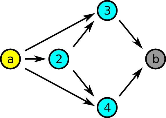
Schedule

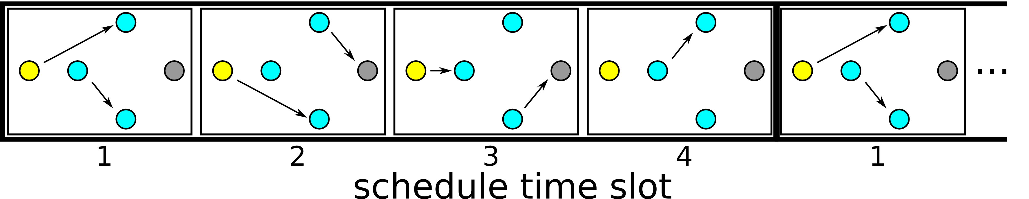
Figure 6: Example of a simple mesh network for network estimation.

The packet delivery predictions from the network estimator are shown in Figure 7. Although the network estimator provides $f_{\bm{\nu}_{{}^{k}}^{{}_{k+H-1}}}(\bm{\tilde{\nu}}_{{}^{0}}^{{}_{H-1}})$, at each sample time $k$ we plot the average prediction $\operatorname*{{\mathbb{E}}}[\bm{\nu}_{{}^{k}}^{{}_{k+H-1}}]$. In this example, all the links are up for $k\in\{1,\ldots,4\}$ and then link $(3,b)$ fails from $k=5$ onwards. After seeing a packet loss at $k=5$, the network estimator revises its packet delivery predictions and now thinks there will be a packet loss at $k=7$. The average prediction for the packet delivery at a particular sample time tends toward 1 or 0 as the network estimator receives more information (in the form of packet deliveries) about the new state of the network.

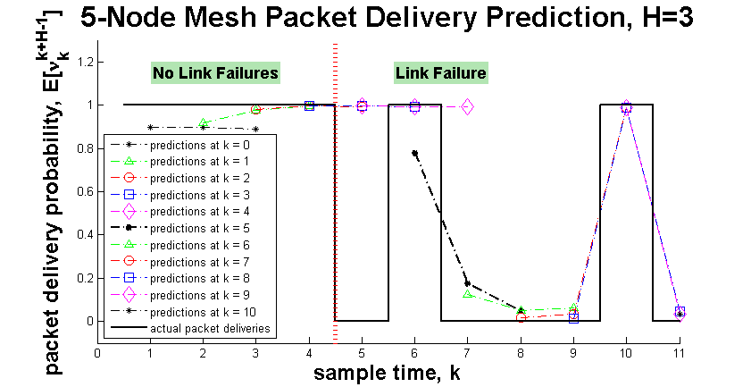
Figure 7: Packet delivery predictions when network in Figure 6 has all links up and then link $(3,b)$ fails.

The prediction for $k=7$ (packet generated at schedule time slot 3) at $k=5$ is influenced by the packet delivery at $k=5$ (packet generated at schedule time slot 1) because hop-by-hop routing allows the packets to traverse the same links under some realizations of the underlying routing topology $G$. Mesh networks with many interleaved paths allow packets generated at different schedule time slots to provide information about each others’ deliveries, provided the links in the network have some memory. As discussed in Section 3.4, since a packet delivery provides only one bit of information about the network state, it may take several packet deliveries to get good predictions after the network changes.

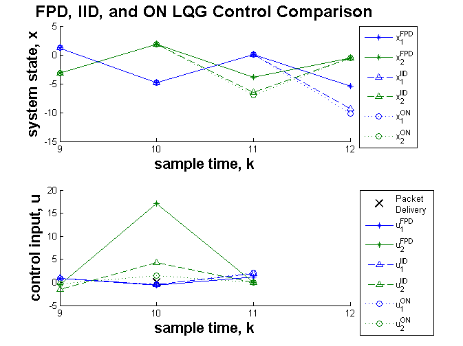
Figure 8: Plot of the different control signals and state vectors when using the FPD controller, an IID controller, and an ON controller (see text for details).

Now, consider a linear plant with the following parameters

$$A=\left[\begin{array}[]{cc}0&1.5\\ 1.5&0\end{array}\right],B=\left[\begin{array}[]{cc}5&0\\ 0&0.2\end{array}\right],R_{w} =\left[\begin{array}[]{cc}0.1&0\\ 0&0.1\end{array}\right],R_{0}=\left[\begin{array}[]{cc}10&0\\ 0&10\end{array}\right]$$

$$Q_{1}=Q_{2}=\left[\begin{array}[]{cc}1&0\\ 0&1\end{array}\right],Q_{n} =\left[\begin{array}[]{cc}10&0\\ 0&10\end{array}\right]\quad.$$

The transfer matrix $A$ flips and expands the components of the state at every sampling instant. The input matrix $B$ requires the second component of the control input to be larger in magnitude than the first component to have the same effect on the respective component of the state. Also, the final state is weighted more than the other states in the cost criterion. We compare the three finite horizon LQG controllers discussed in Section 4, namely the FPD controller, the IID controller, and the ON controller with their costs (15) and (16a).

The controllers are connected to the plant at sample times $k=9,10,11$ through the network example given in Figure 7. Figure 8 shows the control signals computed by the different controllers and the plant states when the control signals are applied following the actual packet delivery sequence. From the predictions at $k=8,9,10$ in Figure 7, we see that the FPD controller has better knowledge of the packet delivery sequence than the other two controllers. The FPD controller uses this knowledge to compute an optimal control signal that outputs a large magnitude for the second component of $u_{10}$, despite the high cost of this signal. The IID and ON controllers believe the control packet is likely to be delivered at $k=11$ and choose, instead, to output a smaller increase in the first component of $u_{11}$, since this will have the same effect on the final state if the control packet at $k=11$ is successfully delivered.

The FPD controller is better than the other controllers at driving the first component of the state close to zero at the end of the control horizon, $k=12$. Thus, the packet delivery predictions from the network estimator help the FPD controller significantly lower its LQG cost, as shown in Table 1. The costs reported here are obtained from Monte-Carlo simulations of the system, averaged over 10,000 runs, but with the network state set to the one described above.

Table 1: Simulated LQG Costs (10,000 runs) for Example Described in Section 5

FPD Controller	IID Controller	ON Controller
681.68	1,008.2	1,158.9

6 Discussion on Network Model Selection

The ability of the network estimator to accurately predict packet deliveries is dependent on the network model. A natural objection to the GEIHS network model is that it assumes links are independent and does not capture the full behavior of a lossy and bursty wireless link through the G-E link model [15]. Why not use one of the more sophisticated link models mentioned by Willig et al. [15]? Why not use a network model that can capture correlation between the links in the network? A good network model must be rich enough to capture the relevant behavior of the actual network, but not have too many parameters that are difficult to obtain.

In our problem setup, the relevant behavior is the packet delivery sequence of the network. As mentioned in Section 3.4, the network state probability distribution does not need to identify the exact network topology realization to get precise packet delivery predictions. In this regard, the GEIHS network model has too many states ($2^{E}$ states) and may be overmodeling the actual network. However, the more relevant question is: Does the GEIHS network model yield accurate packet delivery predictions, predictions that are close to the actual future packet delivery sequence? Do the simplifications from assuming link independence and using a G-E link model result in inaccurate packet delivery predictions? These questions need further investigation, involving real-world experiments.

Our GEIHS network model has as parameters the routing topology $G$, the schedule $\mathbf{F}^{(T)}$, the G-E link transition probabilities $\{p_{l}^{\mathrm{u}},p_{l}^{\mathrm{d}}\}_{l\in{\mathcal{E}}}$, the source $a$, the sink $b$, the packet generation times $t_{k}$, and the deadlines $t_{k}^{\prime}$. The most difficult parameters to obtain are the link transition probabilities, which must be estimated by link estimators running on the nodes and relayed to the GEIHS network estimator. Furthermore, on a real network these parameters will change over time, albeit at a slower time scale than the link state changes. The issue of how to obtain these parameters is not addressed in this paper.

Despite its limitations, the GEIHS network model is a good basis for comparisons when other network models for our problem setup are proposed in the future. It also raises several related research questions and issues.

Are there classes of routing topologies where packet delivery statistics are less sensitive to the parameters in our G-E link model $p_{l}^{\mathrm{u}}$ and $p_{l}^{\mathrm{d}}$? How do we build networks (e.g., select routing topologies and schedules) that are “robust” to link modeling error and provide good packet delivery statistics (e.g., low packet loss, low delay) for NCSs? The latter half of the question, building networks with good packet delivery statistics, is partially addressed by other works in the literature like Soldati et al. [19], which studies the problem of scheduling a network to optimize reliability given a routing topology and packet delivery deadline.

Another issue arises when we use a controller that reacts to estimates of the network’s state. In our problem setup, if the network estimator gives wrong (inaccurate) packet delivery predictions, the FPD controller can actually perform worse than the ON controller. How do we design FPD controllers that are robust to inaccurate packet delivery predictions?

7 Conclusions

This paper proposes two network estimators based on simple network models to characterize wireless mesh networks for NCSs. The goal is to obtain a better abstraction of the network, and interface to the network, to present to the controller and (future work) network manager. To get better performance in a NCS, the network manager needs to control and reconfigure the network to reduce outages and the controller needs to react to or compensate for the network when there are unavoidable outages. We studied a specific NCS architecture where the actuation channel was over a lossy wireless mesh network and a network estimator provided packet delivery predictions for a finite horizon, Future-Packet-Delivery-optimized LQG controller.

There are several directions for extending the basic problem setup in this paper, including those mentioned in Sections 3.3, 3.4, and 6. For instance, placing the network estimator(s) on the actuators in the general system architecture depicted in Figure 1 is a more realistic setup but will introduce a lossy channel between the network estimator(s) and the controller(s). Also, one can study the use of packet delivery predictions in a receding horizon controller rather than a finite horizon controller.

References

- [1] Wireless Industrial Networking Alliance, “WINA website,” http://www.wina.org, 2010.
- [2] International Society of Automation, “ISA-SP100 wireless systems for automation website,” http://www.isa.org/isa100, 2010.
- [3] I. Chlamtac, M. Conti, and J. J. N. Liu, “Mobile ad hoc networking: Imperatives and challenges,” Ad Hoc Networks, vol. 1, no. 1, pp. 13–64, 2003.
- [4] R. Bruno, M. Conti, and E. Gregori, “Mesh networks: commodity multihop ad hoc networks,” IEEE Communications Magazine, vol. 43, no. 3, pp. 123–131, Mar. 2005.
- [5] J. P. Hespanha, P. Naghshtabrizi, and Y. Xu, “A survey of recent results in networked control systems,” Proc. of the IEEE, vol. 95, pp. 138–162, 2007.
- [6] C. Robinson and P. Kumar, “Control over networks of unreliable links: Controller location and performance bounds,” in Proc. of the 5th International Symposium on Modeling and Optimization in Mobile, Ad Hoc, and Wireless Networks (WiOpt), Apr. 2007, pp. 1–8.
- [7] L. Schenato, B. Sinopoli, M. Franceschetti, K. Poolla, and S. S. Sastry, “Foundations of control and estimation over lossy networks,” Proc. of the IEEE, vol. 95, pp. 163–187, 2007.
- [8] H. Ishii, “ control with limited communication and message losses,” Systems & Control Letters, vol. 57, no. 4, pp. 322–331, 2008.
- [9] P. Seiler and R. Sengupta, “An approach to networked control,” IEEE Transactions on Automatic Control, vol. 50, pp. 356–364, 2005.
- [10] N. Elia, “Remote stabilization over fading channels,” Systems & Control Letters, vol. 54, no. 3, pp. 237–249, 2005.
- [11] R. Olfati-Saber, J. Fax, and R. Murray, “Consensus and cooperation in networked multi-agent systems,” Proc. of the IEEE, vol. 95, no. 1, pp. 215–233, Jan. 2007.
- [12] V. Gupta, A. Dana, J. Hespanha, R. Murray, and B. Hassibi, “Data transmission over networks for estimation and control,” IEEE Trans. on Automatic Control, vol. 54, no. 8, pp. 1807–1819, Aug. 2009.
- [13] D. Varagnolo, P. Chen, L. Schenato, and S. Sastry, “Performance analysis of different routing protocols in wireless sensor networks for real-time estimation,” in Proc. of the 47th IEEE Conference on Decision and Control, Dec. 2008.
- [14] K. S. J. Pister and L. Doherty, “TSMP: Time synchronized mesh protocol,” in Proc. of the IASTED International Symposium on Distributed Sensor Networks (DSN), Nov. 2008.
- [15] A. Willig, M. Kubisch, C. Hoene, and A. Wolisz, “Measurements of a wireless link in an industrial environment using an ieee 802.11-compliant physical layer,” IEEE Trans. on Industrial Electronics, vol. 49, no. 6, pp. 1265–1282, Dec. 2002.
- [16] P. Smyth, D. Heckerman, and M. I. Jordan, “Probabilistic independence networks for hidden markov probability models,” Neural Comput., vol. 9, no. 2, pp. 227–269, 1997.
- [17] R. Castro, M. Coates, G. Liang, R. Nowak, and B. Yu, “Network tomography: Recent developments,” Statistical Science, vol. 19, no. 3, pp. 499–517, Aug. 2004.
- [18] K. J. Åström, Introduction to Stochastic Control Theory. Academic Press, 1970, republished by Dover Publications, 2006.
- [19] P. Soldati, H. Zhang, Z. Zou, and M. Johansson, “Optimal routing and scheduling of deadline-constrained traffic over lossy networks,” in Proc. of the IEEE Global Telecommunications Conference, Miami FL, USA, Dec. 2010.