Simulation of melting of two dimensional Lennard-Jones solids

Abstract

We study the nature of melting of a two dimensional (2D) Lennard-Jones solid using large scale Monte Carlo simulation. We use systems of up to 102,400 particles to capture the decay of the correlation functions associated with translational order (TO) as well as the bond-orientational (BO) order. We study the role of dislocations and disclinations and their distribution functions. We computed the temperature dependence of the second moment of the TO order parameter ($\Psi_{G}$) as well as of the order parameter $\Psi_{6}$ associated with BO order. Applying finite-size scaling of these second moments we determined the anomalous dimension critical exponents $\eta(T)$ and $\eta_{6}(T)$ associated with power-law decay of the $\Psi_{G}$ and $\Psi_{6}$ correlation functions. We also computed the temperature dependent distribution of the order parameters $\Psi_{G}$ and $\Psi_{6}$ on the complex plane which support a two stage melting with a hexatic phase as an intermediate phase. From the correlation functions of $\Psi_{G}$ and $\Psi_{6}$ we extracted the corresponding temperature dependent correlation lengths $\xi(T)$ and $\xi_{6}(T)$. The analysis of our results leads to a consistent picture strongly supporting a two stage melting scenario as predicted by the Kosterlitz, Thouless, Halperin, Nelson, and Young (KTHNY) theory where melting occurs via two continuous phase transitions, first from solid to a hexatic fluid at temperature $T_{m}$, and then from the hexatic fluid to an isotropic fluid at a critical temperature $T_{i}$. We find that $\xi(T)$ and $\xi_{6}(T)$ have a distinctly different temperature dependence each diverging at different temperature and that their finite size scaling properties are consistent with the KTHNY theory. We also used the temperature dependence of $\eta$ and $\eta_{6}$ and their theoretical bounds to provide estimates for the critical temperatures $T_{m}$ and $T_{i}$, which can also be estimated using the Binder ratio. Our results are within error bars the same as those extracted from the divergence of the correlation lengths.

I Introduction

The most widely considered theory of 2D melting is the so-called KTHNY theory of Kosterlitz and Thouless KT , Halperin and Nelson HN ; NH , and Young Young , which predicts that melting in two dimensions occurs via two continuous phase transitions, first from solid to hexatic fluid, and then from hexatic fluid to isotropic fluid. This theory begins from the fact that true translational order cannot exist at any non-zero temperature in 2D because of the infrared divergence caused by the zero point motion of long-wave-length density fluctuations. According to the KTHNY theory, another form of true long-range order exists below some non-zero temperature $T_{m}$ where only the directions of the nearest-neighbor bonds order. This long-range bond order disappears above $T_{m}$ because of dislocation unbinding which leads to an intermediate phase, the hexatic phase, characterized by topological order, where while dislocations are unbound, disclinations with opposite topological charge remain bound. These disclinations become unbound at a higher temperature $T_{i}$ where the system becomes an isotropic disordered fluid.

Simulation of melting in classical two-dimensional (2D) systems has been tackled by means of a variety of computational studiesKrauth for several decades without reaching a definite conclusion regarding its nature. In particular for hard disks in 2D, a large number of computer simulation studies have been applied to understand 2D melting, since this is the toy model on which the Metropolis Monte Carlo method itself was first introducedMetropolis and soon afterward, the 2D melting of hard disks was studiedDisks . One of the reasons for the difficulty to reach an unequivocal conclusion is that in 2D a conventional solid with true translational order cannot exist, and, instead the correlations decay very slowly over long distance. This requires large size systems where the relaxation time scales become very long for these types of phenomena. In particular for hard disk systems, when using a local updating algorithm or even molecular dynamics, particles remain stuck in their local “cage” for large computational time scales, precisely because of the hard disk constraint.

One might think that Monte Carlo simulation of soft-core potentials, such as the Lennard-Jones system in 2D, might not be plagued by the same level of computational severity as the hard-disk systems, because of the softening of the hard-core constraint. As a matter of fact there are a number of studies of the Lennard-Jones solidChester by computer simulation where also a general consensus about the nature of melting has not been established. Some studies have favored a first-order transition from solid to liquid Toxvaerd ; Abraham ; Bakker ; Chester84 , as predicted by the grain boundary melting suggestionChui , while other studies Frenkel ; Udink ; Somer ; Somer98 have leaned toward the KTHNY theory. The most thorough of these studies, however, are at least one decade old and because of the fact that the computational resource constraints of today are significantly better, a more thorough study should be possible.

In the present paper, we study the nature of melting of a two dimensional (2D) Lennard-Jones solid using large scale Monte Carlo simulation. We use systems of up to 102,400 particles to capture the decay of the correlation functions associated with translational as well as the bond-orientational order. We find that to carry out thorough investigations beyond these sizes, calculations using the Metropolis local update become impractical using today’s high performance computing because of the long relaxation time scales. Further technical details of our simulation are described in the next section, and the remainder of the paper is organized as follows. In Sec. III we discuss the role of defects in the KTHNY theory of melting and present the results of a geometric defect analysis. In Sec. IV we show the temperature dependence of both order parameters, $\Psi_{G}$ and $\Psi_{6}$, as well as their second moments, $\Psi_{G}^{2}$ and $\Psi_{6}^{2}$. The system-size dependence of $\Psi_{G}^{2}$ and $\Psi_{6}^{2}$ can be used to determine the critical exponents $\eta$ and $\eta_{6}$, as shown in Sec. V. In the same section, the KTHNY values of the critical exponents at melting, $\eta(T_{m})$ and $\eta_{6}(T_{i})$, are used to estimate the transition temperatures $T_{m}$ and $T_{i}$. Next, in Sec. VI, we present our results on the correlation function associated with bond orientational order above $T_{i}$ and determine the temperature dependent correlation length $\xi_{6}(T)$. In the same section, we demonstrate finite-size scaling of $\Psi_{6}^{2}$. A similar presentation is given in Sec. VII for the pair distribution function and the correlation length of translational order, $\xi(T)$. In addition, we present our findings for the scaling behavior of the second moment of $\Psi_{G}^{2}$ in this same section. Sec. VIII presents an analysis of the melting transition using Binder’s cumulant ratio Binder81 for each order parameter, and also includes a discussion of finite-size scaling theory in the presence of multiple correlation lengths. Finally, in Sec. IX, we give a brief summary of our main findings and conclusions.

II Simulation details

In the Lennard-Jones potential, for two particles separated by a distance $r$,

$$V(r)=4\epsilon\left(\left(\frac{\sigma}{r}\right)^{12}-\left(\frac{\sigma}{r}\right)^{6}\right),$$ (1)

an attractive inverse sixth power tail is combined with a repulsive inverse twelfth power hard core, such that there are only two parameters: $\epsilon$, the potential well depth, and $\sigma$, the hard-core diameter. However, our results can be inferred for any particular value of these parameters (for a specific real system), since in our calculations, distance is measured in units of $\sigma$ and temperature in units of $\epsilon/k_{B}$.

In our calculations we have truncated the Lennard-Jones potential at a distance of 3$\sigma$, and shifted the value of the potential within this cutoff distance by a constant so that the resulting potential approaches zero at 3$\sigma$ (matching the values beyond 3$\sigma$). This truncation is justified because the Lennard-Jones potential is already quite small (-0.005$\epsilon$) at this distance, and is not expected to significantly affect the accuracy of our simulations. Additionally, by using a cutoff distance, we are able to use a cell list structure in our algorithms so that our computations scale as $O(N)$ instead of the $O(N^{2})$ scaling without a cutoff distance ($N$ is the number of particles in our simulation cell).

We have collected data for systems of 1600, 6400, and 25600 particles over a wide temperature range at a density of 0.873. Additionally, we have simulated a system of 102400 particles for three temperature values at the same density in order to verify our results for the smaller system sizes. To accommodate the expected low temperature triangular solid phase, a periodic simulation cell of proportion 2:$\sqrt{2}$ is used. We have performed our calculations on the Florida State University shared High-Performance Computing facility, which contains several thousand compute nodes. The processors on these nodes range in speed from 2.3 GHz to 2.8 GHz, and it takes about 34 hours to perform 1,000,000 Monte Carlo sweeps for $N=25600$ particles, including calculating observables every 100 Monte Carlo sweeps (MCS). We have found that, except for the $N=102,400$ particle system, a million MCS are sufficient to reach equilibrium, even near the critical points. The data presented here is obtained over one million MCS, after a period of one (for $N=102,400$) or two (for $N=1600,6400$, and 25600) million MCS of equilibration.

To take advantage of our computational resources, we utilized a trivially parallel Monte Carlo implementation of 100 threads, each with a unique random number seed and initial configuration. Simulations begin from an initial near-ordered configuration (particles are placed in a triangular lattice, with 5% lattice spacing random fluctuations). Statistics for thermodynamic variables are collected by generating averages on each of the 100 parallel threads, then using the central limit theorem we obtain the total average, as we have 100 independent means.

Although in our preliminary studies we have computed thermodynamic quantities for a range of densities and temperatures, the effects of critical slowing down near the melting transition and our desire to study the largest possible systems have led us to focus on a single density, 0.873 (all densities are in units of particles per $\sigma^{-2}$). This density was chosen for several reasons. This is a density that could be readily compared to prior numerical simulations of Lennard-Jones melting Udink . Also, we wanted a density that is relatively low, but large enough to avoid the solid-vapor coexistence phase at low temperatures. Strictly speaking, there is a solid phase in the zero temperature limit only at densities of 0.9165 (the density at which the spacing of the triangular lattice is the same as the position of the Lennard-Jones potential minimum) and above. Below this density there is a solid-vapor coexistence phase. However, the triple point density is roughly 0.82, so at higher densities the system will in general become solid before the onset of melting occurs Chester .

III Role of defects

III.1 Defect types

In two dimensions, the densest packing of particles of uniform size is achieved in a triangular lattice. In such a configuration, each particle has exactly six nearest neighbors. Thermal fluctuations will lead to distortions in the lattice, or even destroy it completely. To quantify this, we use the Delaunay triangulation to determine the nearest neighbor network of our particle configurations. The nearest neighbor network tells us the number of nearest neighbors, or coordination number, of each particle. For a system of particles in a periodic plane, the average coordination number is always six Allen . Particles in a triangularly ordered region will be six-coordinated, while disruptions in the lattice will lead to particles with coordination numbers greater than or less than six. A defect is defined as any coordination number other than six. These non-six-coordinated atoms may be thought of as disclinations of charge ${\bf n}$, their coordination number being $6+{\bf n}$.

The most common type of disruption, or defect, is a five- or seven-coordinated particle. These may be interpreted as disclinations of charge plus or minus one. Two oppositely charged disclinations may be thought of as a dislocation. More complex arrangements of disclinations are possible, such as dislocation pairs and grain boundary loops, but in our analysis we have only considered individual defects. The defect fraction, $f_{d}=1-N_{6}/N$, is defined as the fraction of particles that do not have six neighbors, where $N$ is the number of particles in the system, and $N_{6}$ is the number of six-coordinated particles in the system. Remembering that dislocations are made of two bound disclinations of opposite charge, and that dislocations become unbound above the melting point, we can expect the defect fraction to experience a jump at the melting point Allen . Additionally, at low temperatures we can expect an energy gap to occur, which is the energy cost to create a dislocation pair. Because the overall disclinicity of the system must be zero, as well as the net Burgers vector of any dislocations, the lowest-energy defect excitation is a dislocation pair of opposite Burgers vectors. In practice this is usually two pairs of 5- and 7-coordinated particles. This leads to an exponential behavior in the defect fraction, $f_{d}=e^{-\beta\Delta}$, where $\Delta$ is the lowest-energy for a defect type excitation of the system.

III.2 Unbinding of defects

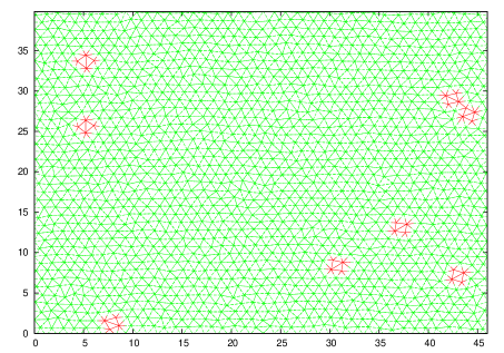
Figure 1: The Delaunay triangulation for $N=1600$ particles at T=0.70. Defects are shown in red.

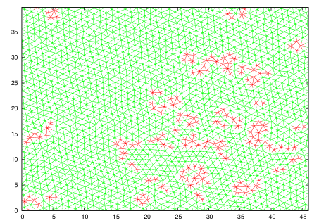
Figure 2: The Delaunay triangulation for $N=1600$ particles at T=0.90. Defects are shown in red.

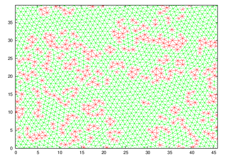
Figure 3: The Delaunay triangulation for $N=1600$ particles at T=1.10. Defects are shown in red.

In Figures 1,2,3 the Delaunay triangulated configuration of a 1600 particle system is shown at temperatures 0.7, 0.9 and 1.1 respectively. The defects are shown in red. At low temperature as demonstrated in Figure 1, we see that defects occur in quadruplets consisting of two 5-coordinated and two 7-coordinated particles. As the temperature is raised to 0.9 (Figure 2) we can see isolated dislocations (one 5-fold coordinated atom bound to a 7-fold coordinated atom). At yet higher temperature, such as 1.1 (Figure 3) we can observe isolated disclinations.

This can also be seen in the pair distribution functions $g_{77}(r)$, $g_{55}(r)$, and $g_{57}(r)$, for pairs of 7-coordinated particles, pairs of 5-fold coordinated atoms and for 5-fold-7-fold coordinated atoms respectively. In Figure 4, a sharp peak in $g_{77}(r)$ is observed at low temperatures ($T=0.70$), indicating that dislocations are tightly bound. At higher temperatures ($T=0.90$ and $T=1.10$), the peak in $g_{77}(r)$ is greatly diminished, and dislocations become first weakly bound ($T=0.90$) and then completely unbound ($T=1.10$). $g_{55}(r)$, while not shown, behaves qualitatively similar to $g_{77}(r)$, as both are representative of the pair distribution of dislocations.

Figure 4: The pair distribution function for 7-coordinated particles, $g_{77}(r)$. The peak for T=0.70 extends to $\sim 50$.

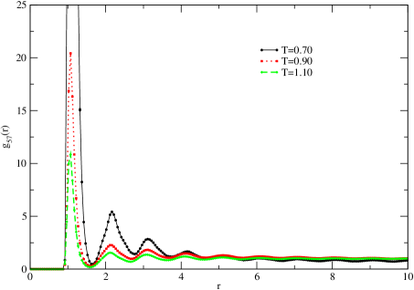
Figure 5: The pair distribution function for pairs consisting of one 5-coordinated particle and one 7-coordinated particle, $g_{57}(r)$. The peak for T=0.70 extends to $\sim 150$.

The pair distribution function for disclinations, $g_{57}(r)$, is shown in Figure 5. While the sharp peak at low ($T=0.70$) and intermediate ($T=0.90$) temperature is expected, the peak at $T=1.10$, while quite lower, is still very substantial. This indicates that disclinations have not become completely unbound, and indeed it is difficult to find isolated disclinations in the snapshot configurations presented in Figure 3. When isolated disclinations do occur, they are still next-nearest neighbors with at least one other disclination of opposite charge.

III.3 Defect fraction

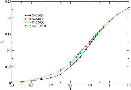
Figure 6: Fraction of defects, $f_{d}$, as defined by the fraction of non-six-coordinated particles in the Delaunay triangulation, $f_{d}=1-N_{6}/N$. The rapid rise in $f_{d}$ from near zero to almost 25% is a possible sign that dislocation and/or disclination unbinding is occurring.

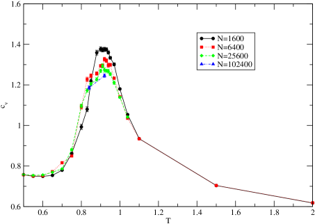
Figure 7: The presence of a peak in the specific heat is indicative of a phase transition. Interestingly, the peak near $T=0.9$ appears to lessen in magnitude as the system size is increased.

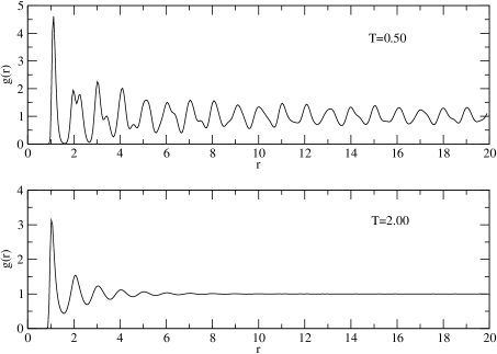
Figure 8: The distribution function shows ordering at low temperatures, as shown above for $T=0.50$, while at higher temperatures, such as T=2.00 shown above, there is a loss of order over moderate length scales.

According to the KTHNY theory, disclinations remain very tightly bound below $T_{m}$. Above $T_{m}$, the disclinations are screened from one another by the presence of free dislocations yet remain bound, albeit by a weaker logarithmic bindingNH . Thus, we expect a proliferation of defects to occur around $T_{m}$, and to continue growing until somewhere above $T_{i}$, where a saturation should occur. In Figure 6 we show the average defect fraction as a function of temperature. At low temperature, there are very few defects, while at high temperature there is a considerable fraction of the system that is defected. In between, there is a region of rapidly increasing defect fraction, from $T=0.8$ to $T=1.0$. This can be quantitatively verified by calculating the temperature derivative of the defect fraction, which is indeed found to have a broad peak in this temperature region. The overall shape of $df_{d}(T)/dT$ is very similar to that of the specific heat capacity, to be shown next. Additionally, we can see some size dependence in the region $0.6<T<1.0$, although this seems to be an issue mostly for comparisons of the smallest system size ($N=1600$) to the larger system sizes.

The specific heat per particle at constant volume, $c_{V}$, can be calculated from the energy fluctuations,

$$c_{V}={1\over N}{{\langle E^{2}\rangle-\langle E\rangle^{2}}\over{k_{B}T^{2}}}$$ (2)

where $E$ is the total energy of an $N$ particle system. We have calculated the specific heat and show it as a function of temperature in Figure 7. One can see a broad peak in the specific heat per particle. According to the KTHNY theory, there should be an essential singularity in the specific heat at both $T_{m}$ and $T_{i}$NH . However, it is not clear whether this will be visible above background contributions to the specific heat. Either way, the peak in specific heat points to a rearrangement of order in the systems studied. Also, if we look at the distribution function (Figure 8), we see ordering at low temperatures, and fluid behavior at high temperatures. Overall, it is clear that there is a phase transition occurring, with a disordered fluid state at high temperatures and an ordered state at low temperatures.

III.4 Defect excitation energy

In the KTHNY theory, dislocations are bound at low temperatures, and there is a defect core energy associated with their creation. This leads to an energy gap, and thus using the Arrhenius law, we expect $f_{d}=e^{-2E_{c}/k_{B}T}$, where we have used $2E_{c}$ because dislocation pairs are the lowest energy excitation (isolated dislocations are forbidden). In Table 1 we show the defect activation energy as calculated by the Arrhenius law at low temperatures. Taking the low temperature limit, we find $E_{c}=1.49\pm 0.01$.

Temperature	N=1600	N=6400	N=25600
0.50	1.49946(30)	1.4919(19)	1.4873(14)
0.55	1.50267(85)	1.4884(31)	1.4778(22)
0.60	1.4996(14)	1.4635(43)	1.4252(31)
0.65	1.4872(26)	1.3908(59)	1.3480(29)
0.70	1.4543(30)	1.2795(49)	1.2835(15)
0.75	1.3640(54)	1.2027(19)	1.2390(26)

Table 1: Defect activation energy for various system sizes and temperatures, as computed using the Arrhenius law. The numbers in parentheses are the uncertainty of the trailing digits.

IV Order parameters

IV.1 Definition and temperature dependence

Let us define a global order parameter of translational order,

$$\Psi_{\vec{G}}=\frac{1}{N}\sum_{j=1}^{N}\exp\left(i\vec{G}\cdot\vec{r_{j}}\right),$$ (3)

where $\vec{G}$ is a reciprocal lattice vector, and $\vec{r_{j}}$ is the position vector of particle $j$. If there is translational ordering in a system, then clearly $\Psi_{\vec{G}}$ will be non-zero if $\vec{G}$ is a reciprocal lattice vector of the appropriate lattice geometry. Due to the shape of our simulational cell, at low temperatures this will be a triangular lattice with nearest-neighbors in the x-direction. At high temperatures, no translational ordering is present, and all possible values of $\vec{G}$ should give the same (qualitative) result. However, at intermediate temperatures, it may be possible for there to be some degree of translational ordering that is not strictly commensurate with our simulation cell. Indeed, we have observed “canted” solid phases at intermediate temperatures, where we find partial triangular order with nearest neighbors in a direction titled from the x-axis by a small angle. In this case, if $\vec{G}$ for the triangular order commensurate with our simulation cell is used, $\Psi_{\vec{G}}$ will be found to be zero. However, if we use an appropriate $\vec{G}$ for the order present, $\Psi_{\vec{G}}$ will be found to be non-zero. For this reason, we define the true translational order to be the maximum value of $\Psi_{\vec{G}}$ for all $\vec{G}$. In practice, it is not possible to perform this optimization for each Monte Carlo configuration, so we make the following assumptions. First, due to the nature of ordering in two dimensions, we assume any lattice will be triangular. Second, because the density of particles is fixed, we assume the lattice spacing in said triangular solid to be the same as that for the commensurate cell. Thus, we keep the magnitude of $\vec{G}$ constant, and simply determine the direction of solid ordering for each configuration by looking at the average bond direction between nearest neighbor particles. This turns out to be a good estimate of the true translational order for a system, but it must be remembered that it is strictly speaking a lower bound.

The local order parameter which measures the degree of six-fold orientational ordering is defined as

$$\psi_{6}(\vec{r}_{i})={1\over{n(i)}}\sum_{j=1}^{n(i)}e^{i6\theta_{ij}}\$$ (4)

where $\theta_{ij}$ is the angle of the bond between particles $i$ and $j$ and the sum over $j$ extends over all $n(i)$ nearest neighboring atoms found by the Delaunay triangulation. The global order parameter associated with bond-orientational order is obtained as an average over all particles.

$$\Psi_{6}={1\over N}\sum_{i=1}^{N}\psi_{6}(\vec{r}_{i}).$$ (5)

In a perfectly bond-ordered triangular solid, we have that $n(i)=6$ and $\theta_{ij}=\pi/3$ for all $j=1,..,6$. In such case $|\langle\Psi_{6}\rangle|=1$. In the low temperature phase, there is bond-orientational order, so $\langle\Psi_{6}\rangle$ should be a point on the perimeter of a circle with a radius approaching unity as $T\to 0$. In the hexatic phase there is quasi-long-range bond-orientational order, which implies that the distribution of $\langle\Psi_{6}\rangle$ should become a ring in the imaginary plane. In the isotropic phase both $\langle\Psi_{6}\rangle$ and $\langle\Psi_{\vec{G}}\rangle$ should be distributed around zero value.

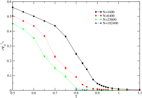
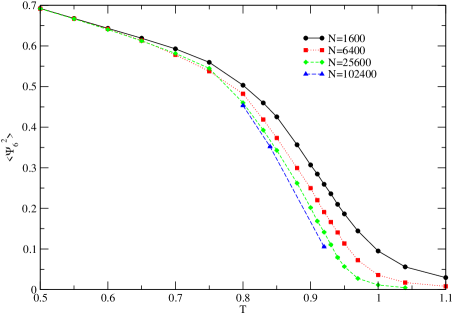
Figure 9: The second moment of the translational (top) and bond orientational (bottom) order parameters.

In the top panel of Figure 9 we show the second moment of the translational order parameter, $\Psi_{G}^{2}$ . There appears to be a transition from a translationally ordered phase at low temperatures to a disordered phase at higher temperatures. In the ordered phase there is a clear relation between $\Psi_{\vec{G}}^{2}$ and system size. We will explore this relation in a later section, but for now let us point out that this finite-size scaling relation begins to break down above $T=0.60$. This is expected within the KTHNY theory of melting due to the unbinding of dislocations. However, on closer inspection, the behavior of the curves for $N=6400$ and $N=25600$ in the region $0.6<T<0.8$ is not a smooth connection of the data at higher and lower temperature. This is due to our measured quantity $\Psi_{G}$ being a lower bound of translational order.

Also shown in Figure 9 is the second moment of the bond orientational order parameter, $\Psi_{6}^{2}$ (bottom panel). At low temperatures there is substantial bond orientational order. Below $T=0.70$ there is very little dependence of $\Psi_{6}^{2}$ on system size. As the temperature is increased, $\Psi_{6}^{2}$ begins to show a marked dependence on system size as well as a steep decline in value as we approach the high temperature disordered phase.

IV.2 Order parameter distribution

The main prediction of Halperin and NelsonHN ; NH and YoungYoung is that if two dimensional melting is the result of dislocation unbinding, as proposed by Kosterlitz and ThoulessKT , then a second unbinding transition (of disclinations) is required to reach an isotropic fluid state. This implies the presence of a novel hexatic fluid phase. In Figure 10 we show an intensity plot of the distribution of $\Psi_{\vec{G}}$ and of $\Psi_{6}$ on the complex plane for three different temperatures.

At $T=0.70$ (top row), our calculation of the distribution of the order parameters finds a ring of values for $\Psi_{\vec{G}}$, while $\Psi_{6}$ is localized in a small region away from the origin (a very narrow peak showing as a “star” along the positive real axis). This is consistent with the presence of long-range bond orientational order ($|\langle\Psi_{6}\rangle|>0$), while the ring of $\Psi_{\vec{G}}$ values is expected for quasi-long-range translational order. At $T=0.90$ (middle row), we that $\Psi_{\vec{G}}$ is clustered about the origin, indicating a lack of translational order. Interestingly, $\Psi_{6}$ now shows a ring of values about the origin, indicating quasi-long-range order. This is exactly what is expected of the hexatic fluid phase. Finally, at $T=1.10$ (bottom row) we see that both order parameters are distributed about the origin, indicating an isotropic fluid phase of no order.

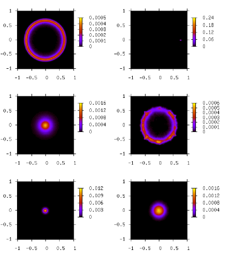
Figure 10: Intensity plots of the probability of $\Psi_{\vec{G}}$ (left column) and $\Psi_{6}$ (right column) on the complex plane for T=0.70 (top row), T=0.90 (middle row), and T=1.10 (bottom row).

V Critical exponents

In the topological solid phase, the scaling form for the second moment of the translational order parameter is $\langle\Psi_{G}^{2}\rangle\sim L^{-\eta}$, where $L$ is the (linear) system size and $\eta$ is a critical exponent. In the hexatic fluid phase, a similar relation holds for bond orientational order, $\langle\Psi_{6}^{2}\rangle\sim L^{-\eta_{6}}$. According to the KTHNY theory of melting, the critical exponents $\eta$ and $\eta_{6}$ will have specific values at melting. The translational critical exponent is bounded at lower melting temperature: $1/4<\eta(T_{m})<1/3$. Additionally, the bond orientational critical exponent grows from zero at $T_{m}$ to 1/4 at $T_{i}$, and is related to the translational correlation length: $\eta_{6}(T)\sim\xi(T)^{-2}$ NH .

By plotting $\langle\Psi_{G}^{2}\rangle$ (or $\langle\Psi_{6}^{2}\rangle$) versus $L$ on a log-log plot, we can find $\eta$ (or $\eta_{6}$). To demonstrate the validity of this scaling law and that our results are not limited by system size, in Figure 11 we plot $\langle\Psi_{6}^{2}\rangle$ versus $\ln L$ for all system sizes at the two temperatures where we have results for the $N=102400$ system. Results of linear least squares fits to the three smallest system sizes (used to generate the data for Figure 12) are shown as a dotted blue line (for data at T=0.80), a dashed red line (for data at T=0.84), and a long-dashed green line (for data at T=0.92). For the higher temperature, the $N=102400$ data falls directly on this line, within error bars. At T=0.84, however, the $N=102400$ data indicates that a smaller value for $\eta_{6}$ at this temperature may be necessary. This could either be due to the (presumably) large translational correlation lengths at this temperature, which would invalidate results for small system sizes, or perhaps a very long relaxation time. Either way, from our data it is clear that by T=0.92 the KTHNY value of $\eta_{6}$ at $T_{i}$ has been well passed.

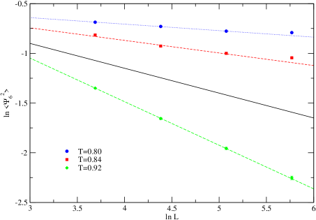
Figure 11: Scaling of $<\Psi_{6}^{2}>$ with system size $L$, shown on a logarithmic plot. Results for T=0.84 are shown as blue circles, while data collected at T=0.92 is represented by red squares. In both cases, the data for the three smaller systems was fit to the equation $\ln<\Psi_{6}^{2}>=-\eta_{6}\ln L+const$, and the result is plotted as the dotted and dashed lines (the solid line is the KTHNY value of $\eta_{6}$ at $T_{i}$). In both cases, the value of $\ln<\Psi_{6}^{2}>$ of the largest system size ($N=102400$) is reasonably close to the value expected from scaling.

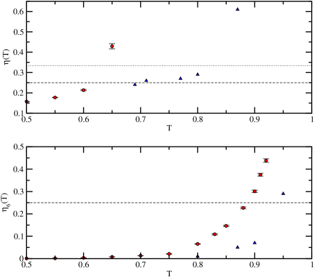
Figure 12: Anomalous dimensionality of (top) the translational order parameter and (bottom) the bond orientational order parameter. Our current results are shown in both figures as red circles. Shown for comparison are the results of Udink and van der Elsken Udink (blue triangles, both figures). In the top figure, the dashed and dotted lines represent the lower and upper bounds of $\eta$ at $T_{m}$, according to KTHNY theory; in the bottom figure, the dashed line represents the predicted value of $\eta_{6}$ at $T_{i}$.

In Figure 12 we show the extracted values of $\eta$ and $\eta_{6}$, the critical exponents of translational and bond orientational order. In both panels, we show our results as red circles. In the top panel, we can see that $\eta$ crosses the KTHNY melting value in the temperature range $0.6<T<0.65$. In the bottom panel we show the critical exponent of bond orientational order, $\eta_{6}$. This exponent crosses the KTHNY melting value (see dashed line) at a temperature near 0.89, in close agreement with the value for $T_{i}$ derived from the divergence of the correlation length $\xi_{6}$ obtained in the next section. This value for $T_{i}$ is also in good agreement with the value reported in Ref. Keola10, . However, in Figure 12 we also show the algebraic exponents reported by Udink and van der ElskenUdink . In both panels, we can see that their values cross the KTHNY melting zone at higher temperatures than our values. We believe this disagreement may be due to insufficient thermalization time in their study, as this could lead to artificially low values of the critical exponents. We should sound a note of caution here in regards to the scaling of $\langle\Psi_{G}^{2}\rangle$. Because our measurements for $\Psi_{G}^{2}$ are lower bounds, it is possible that the extracted exponents $\eta(T)$ are not correct in the temperature regime where $\vec{G}$ is no longer commensurate with the simulation cell, as is the case for $T>0.6$.

VI Correlation Functions

The correlation function for bond orientational order is given by

$$C_{6}(r)=<\psi_{6}(r)\psi_{6}^{*}(0)>,$$ (6)

where $\psi_{6}(\vec{r})$ is the local bond-orientational order parameter defined in Sec. IV. In the isotropic fluid phase, the asymptotic form of $C_{6}(r)$ is $\sim\exp(r/\xi_{6})$ NH . At shorter distances, however, a power law decay comes into play, such that as $\xi_{6}$ diverges as $T_{i}$ is approached from above, then the asymptotic form becomes $C_{6}(r)\sim r^{-\eta_{6}}$ at $T_{i}$ and below, with $\eta_{6}(T_{i})=1/4$. Additionally, we observe oscillations in $C_{6}(r)$ that seem to decay with an exponential envelope. Thus, we used the following fitting form for the bond orientational correlation function for distances $r$ much less than the system size $L$:

$$C_{6}(r)=A{{e^{-r/\xi_{6}}}\over{r^{\eta_{6}}}}+B\sin(kr+\delta){{e^{-r/\xi}}\over{r^{\eta}}}.$$ (7)

We have used a particle-centric definition of the bond orientational correlation function, so in our calculations of $C_{6}(r)$ there will be an influence from $g(r)$, the pair distribution function. In the limit of perfect bond orientational ordering ($\psi_{6}=1$ everywhere), $C_{6}(r)$ and $g(r)$ will be equivalent. We approximate the oscillatory portion of $C_{6}(r)$ which is due to the translational atomic arrangement using a damped oscillator. The periodic form is captured by using $\sin(kr+\delta)$, where k is expected to be near the first reciprocal lattice vector in magnitude ($\sim 6$) and $\delta$ is just a phase-shift parameter. The size of the oscillations are expected to decay exponentially in the fluid phase, and algebraically in the hexatic phase, so we add also a power law, ending up with a term $sin(kr+\delta)r^{-\eta}e^{-r/\xi}$. An example fit is shown in Figure 13. Note that the fitting procedure returns parameters much more precise than the error bars in Figure 13 would indicate are possible. This is due to the high degree of correlation between neighboring points of $C_{6}(r)$. In fact, up to a separation of $3$ the values of $C_{6}(r)$ are still 99% correlated! This simply means that the relative form (including the rate of decay) of $C_{6}(r)$ is consistent between our various calculations, remembering that we average the values of 100 independent parallel Monte Carlo simulations.

We wish to note that we observe an upturn in $C_{6}(r)$ as $r$ approaches $L/2$. At temperatures closer to melting (larger correlation lengths), the upturn occurs further from $L/2$. Next, we would like to determine a characteristic distance $R$ for a given finite-system of linear dimension $L$ so as to stay away from this upturn due to finite-size effects. Namely, we wish to limit the range of $r$ in our fit of the correlation function to the form given by Eq. 7 in the range $\xi_{6}<r<R$. Let us assume a periodic form for the correlation function:

$$C_{6}(r)=A\left(\frac{exp(-r/\xi_{6})}{r^{\eta_{6}}}+\frac{exp(-(L-r)/\xi_{6})}{(L-r)^{\eta_{6}}}\right)$$ (8)

Neglecting the power-law term, the upturn is expected to occur when the $L-r$ terms are a significant fraction of the $r$ terms. Thus,

$$R={L\over 2}-{{\xi_{6}}\over 2}\ln(x)$$ (9)

where $R$ is the distance at which the $L-r$ terms are a fraction $x$ of the $r$ terms. Using $x=0.05$ or 5%, this leads to

$$R={L\over 2}-{{3\xi_{6}}\over 2}.$$ (10)

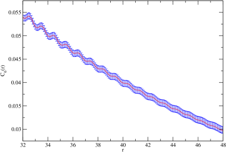
Figure 13: Example of fitting the bond orientational correlation function, $C_{6}$, to the form shown in Equation 7. The data is for $N=25600$ particles at $T=0.97$. The critical exponents are fixed at their maximum values, $\eta=0.33$ and $\eta_{6}=0.25$. The extracted correlation lengths are $\xi=7.40\pm 0.19$ and $\xi_{6}=32.6\pm 0.7$.

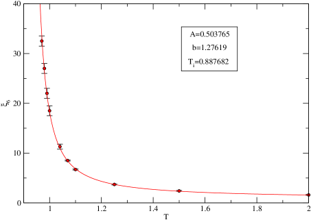
Figure 14: Correlation lengths of the bond orientational order parameter as determined by fitting the bond orientational correlation function to the form mentioned in the text.

In Figure 14 we show $\xi_{6}(T)$ as determined by fitting $C_{6}(r)$ in the range $\xi_{6}<r<R$. These values were fit to the KTHNY form of the expected divergence of $\xi_{6}$ as $T_{i}$ is approached from above: $\xi_{6}(T)=A\exp(b/t^{\nu})$, where $t=(T-T_{i})/T_{i}$ and $\nu=1/2$. This fit gives a value for $T_{i}$ near 0.89.

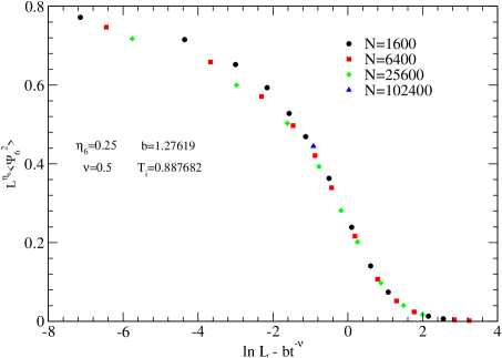
Figure 15: Demonstration of finite-size-scaling by plotting the dimensionless quantity $L^{\eta_{6}}\langle\Psi_{6}^{2}\rangle$ versus $\ln(L/\xi_{6})$, i.e., the logarithm of the ratio of the finite-system-size to the correlation length, for various size systems.

Using the calculated correlation length and critical exponent $\eta_{6}$, in Figure 15 we plot the dimensionless quantity $L^{\eta_{6}}\langle\Psi_{6}^{2}\rangle$ as a function of the dimensionless ratio $\ln(L/\xi_{6})$ for all size-lattice considered here. Notice that the data collapse onto the same scaling function using the same values of the parameters for our fit to $\xi_{6}(T)$ shown in Figure 14, and also setting $\eta_{6}=\eta_{6}(T_{i})=1/4$. This provides additional support for the theory.

VII Distribution functions

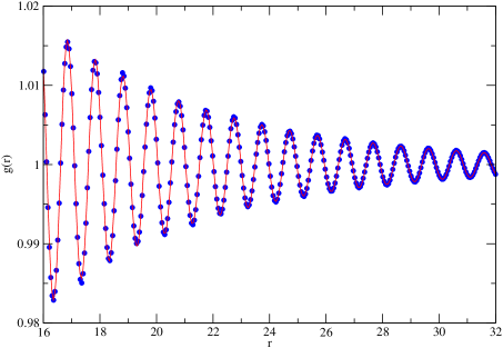
Figure 16: Example of fitting the pair distribution function, $g(r)$, to the form shown in Equation 13. The data is for $N=25600$ particles at $T=0.97$. The critical exponent $\eta$ is fixed at its maximum value, 1/3. The extracted correlation length is $\xi=8.09\pm 0.04$.

In the disordered phase ($T>T_{i}$) the distribution function can be obtained as an angular average of the bond-orientational correlation function $C_{\vec{G}}(\vec{r})$ as

$$g(r)=1+{1\over{2\pi}}\int_{0}^{2\pi}e^{i\vec{G}\cdot\vec{r}}C_{\vec{G}}(\vec{r})d\phi.$$ (11)

The integration of $e^{i\vec{G}\cdot\vec{r}}$ will give us a zeroth-order Bessel function of the first kind, $J_{0}(Gr)$, and using the KTHNY form of the translational correlation function, $C_{\vec{G}}(\vec{r})\sim\exp(-r/\xi)r^{-\eta}$, we wind up with the following form for the radial pair distribution function (in the high temperature limit):

$$g(r\to\infty)=1+AJ_{0}(Gr)e^{-r/\xi}r^{-\eta}$$ (12)

where $A$ is some amplitude.

The $\vec{G}$ that we use here is the same as in the definition of the translational order parameter, namely we use the first reciprocal lattice vector of the idealized triangular lattice that is commensurate with our simulation cell. For the density considered ($\rho\sigma^{2}=0.873$), this means $G\simeq 6.3\sigma^{-2}$. Thus $Gr$ is quite large for moderate values of $r$, and we can use the asymptotic expansion of $J_{0}$, namely $J_{0}(x\to\infty)=\sqrt{2/\pi x}\cos(x-\pi/4)$. Thus in practice we fit $g(r)$ in the disordered phase to the following form,

$$g(r\to\infty)=1+A\cos(kr+\delta){{e^{-r/\xi}}\over{r^{\eta+1/2}}}.$$ (13)

An example fit is shown in Figure 16. In Figure 17 we show the correlation length of translational order as calculated by fitting $g(r)$ to the above form. Results are shown for the $N=25600$ and $N=102400$ particle systems. Clearly, $\xi$ remains finite even as the orientational correlation length diverges. However, there are some discrepancies in our values of $\xi$. At $T=0.92$, the value of $\xi$ extracted from the $N=25600$ particle system does not agree with the value for $N=102400$ particles.

We believe that some of this difference may be attributable to finite size effects. Additionally, there is also the possibility that the $N=102400$ particle system has not fully thermalized. While we have tried to ensure that the data for this largest system is completely thermalized, it can be very difficult to distinguish between stable and metastable states. In either case, we can not consistently fit all the data to the KTHNY form, $\xi=A\exp(b/t^{\nu})$, so instead we have made the fit for only the $N=25600$ data. The result of a fit with $T_{m}=0.61$, $A=0.00311$ and $B=6.62$ using $\nu=0.36963$ is shown in Figure 17 as the red curve. In addition, a few other curves are also shown for different values of these parameters with the same value of $T_{m}=0.61$ whose significance is discussed next.

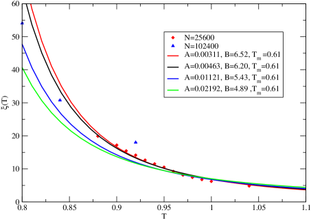
Figure 17: Correlation lengths of the translational order parameter as determined by fitting the pair distribution function to the form mentioned in the text. The range of the fit is from $2\xi$ to $4\xi$, with $\eta$ fixed at its maximum value of 1/3. At $T=0.80$, the fitting range is from $\xi$ to $2\xi$. The solid lines are obtained from the KTHNY form, $\xi=A\exp(b/t^{\nu})$, using $\nu=0.36963$ and various values of the other parameters. Our best fit corresponds to the red curve.

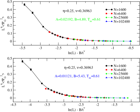
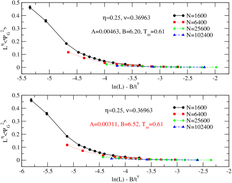
Figure 18: Demonstration of finite-size-scaling by plotting the dimensionless quantity $L^{\eta}\langle\Psi_{G}^{2}\rangle$ versus $\ln(L/\xi)$, i.e., the logarithm of the ratio of the finite-system-size to the measured correlation length, for the two size systems, using $\eta=1/4$ and for various parameters. Due to our calculation of $\langle\Psi_{G}^{2}\rangle$ being a lower bound translational order, only data for $T>0.8$ are shown.

In Figure 18 we show the approximate validity of finite-size scaling by plotting the dimensionless quantity $L^{\eta}\langle\Psi_{G}^{2}\rangle$ versus $\ln(L/\xi)$, i.e., the logarithm of the ratio of the finite-system-size to the measured correlation length, for two different size systems using the lower bound of $\eta=0.25$ according to the KTHNY theory, namely $1/4<\eta<1/3$. The best collapse is obtained for the parameters $A=0.02192$, $B=4.89$ and $T_{m}=0.61$ shown as the top curve in Figure 18. (Note that we have used the constraint $T_{m}>0.6$ as indicated by the behavior of the critical exponent $\eta$). Using the values of the parameters obtained for this “best” collapse we obtain the curve for $\xi(T)$ shown as a green line in Fig. 17. The collapse obtained by using the parameters obtained by the best fit to the correlation length (corresponding to the red curve in Fig. 17) is shown as the graph at the bottom. We have also included two more fits of both types of data, obtained by using parameter values between the above two extremes. We can observe that while we do not obtain the best fit of both sets of data (i.e., collapse of $L^{\eta}\langle\Psi_{G}^{2}\rangle$ versus $\ln(L/\xi)$ (Fig. 18), and the temperature dependence of $\xi(T)$ (Fig. 17) for the same values of these parameters we see that the values of $T_{m}$ and $b$ are close, only the prefactor $A$ cannot be accurately determined. We feel that the overall quality of fit is reasonable given the fact that we had the difficulty discussed above in determining the correlation length associated with translational order.

Several experimental investigations Murray ; Tang have used the decay of the envelope of $g(r)$ to extract $\xi$. The resulting values of $\xi$ appear not to diverge across the melting transition, so perhaps there is some shortfall in using $g(r)$ to get $\xi$ at low temperature. For instance, Murray and Van Winkle observe a finite peak in $\xi$, while for $\xi_{6}$ a divergence is seen to occur Murray .

Regardless of these differences, if we plot the results for $\xi(T)$ on the same plot with the results for $\xi_{6}(T)$ as shown in Figure 19, we see clearly that these two correlation length are very different and the differences between these various fitting forms for $\xi$ are not significant on this scale.

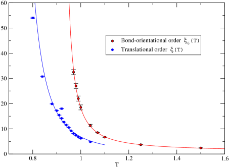
Figure 19: Correlation lengths of the translational order parameter are compared to $\xi_{6}(T)$.

VIII Binder ratios

A central concept in finite-size scaling theory is that any dimensionless quantity should be a function of dimensionless ratios of the finite-size length ($L$) of the system to the correlation length $\xi(T)$ which emerges naturally and it diverges near the critical point Privman90 . Therefore, close enough to the critical point a dimensionless quantity becomes a scaling function $f(L/\xi)$. At precisely the critical point, where the correlation length diverges, all dimensionless quantities are expected to be independent of the system size.

A straightforward way to construct a dimensionless variable is to take the ratio of cumulants. A simple non-trivial ratio is the so-called Binder ratio Binder81 of the fourth and second cumulants,

$$U(x)=1-\frac{\langle(x-\langle x\rangle)^{4}\rangle}{3\langle(x-\langle x\rangle)^{2}\rangle^{2}}.$$ (14)

As mentioned above, this( dimensionless) variable is expected to be system-size independent at a critical point. Hence, if the values of $U(x)$ for several system sizes are plotted across a continuous phase transition, they should cross at the critical point. This is the standard way of estimating for example the critical temperature of a thermal phase transition using the method of Binder ratios.

In the case of melting in two dimensions, however, we have seen that there are two correlation lengths: one for translational order, and another for bond orientational order. Clearly, if we approach very close to either $T_{i}$ or $T_{i}$ only one of these two correlation lengths dominates. For example if we approach $T_{m}$ sufficiently close from above, $\xi$ becomes very large and $\xi_{6}$ is infinite. Thus, there is only one finite correlation length. When we approach $T_{i}$ from above, both $\xi_{6}$ and $\xi$ are finite, but if we are sufficiently close to $T_{i}$, $\xi_{6}\gg\xi$ and so we can neglect the influence of $\xi$. In practice, however, because $\xi_{6}$ grows very rapidly as the temperature $T_{i}$ is approached and we can only study finite-size size systems, the size of $\xi$ is not necessarily negligible as compared to the size of $\xi_{6}$. This implies that the scaling function becomes $f(L/\xi,L/\xi_{6})$. As we have shown in the previous section, $\xi$ is still finite when $\xi_{6}$ diverges at the upper critical temperature, $T_{i}$. Thus, the Binder ratio would only be expected to have a crossing at $T_{i}$ if $\xi\ll L$, which is not the case for the system sizes we have considered ($\xi(T_{i})\approx 20$, half the length of the smallest system size). However, depending on the exact form of the scaling function, there may still be a crossing in the vicinity of $T_{i}$.

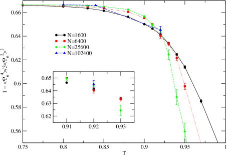
Figure 20: Simplified Keola10 Binder ratio of the bond orientational order parameter (lines are guides for the eye). The inset shows $U(\Psi_{6})$ near the crossing temperature, $T_{c}$.

Looking at the Binder ratio in Figure 20, we can see that there is an apparent crossing of $U(\Psi_{6})$ at $T_{c}=0.92\pm 0.01$. Although our statistical uncertainty is too great to identify the system-size dependence of the Binder ratio crossing (see inset), the finite-size scaling theory outlined above indicates that $T_{c}$ should approach $T_{i}$ when $\xi\ll L$. Thus, while we could use the value of $T_{c}$ as an estimate of $T_{i}$, the method obtained earlier for critical exponents is expected to yield more accurate results to the system sizes considered here.

While we have also calculated $U(\Psi_{G})$, the shortfalls of our estimator for translational order in the temperature region $0.6\leq T\leq 0.8$ lead to an inconclusive analysis of the Binder crossing.

Lastly, let us point out that the finite-size scaling theory discussed in this section should be applicable to any dimensionless parameter. In Sec. VI we demonstrated the scaling collapse of the quantity $L^{\eta_{6}}\langle\Psi_{6}^{2}\rangle$ when plotted as a function of $L/\xi_{6}$. In light of the analysis above, it is clear that we have neglected the $\xi$ dependence of this dimensionless quantity. In Figure 17 we can see that for $T>0.95$ $\xi$ is more or less constant ($\xi\approx 8$). But as $T_{i}$ is approached, $\xi$ increases more rapidly, such that $\xi(T_{i})\approx 20$. This could explain the scatter seen in the scaling collapse of $L^{\eta_{6}}\langle\Psi_{6}^{2}\rangle$ shown in Figure 15.

IX Conclusions

We have shown that several key predictions from the KTHNY theory of two-stage continuous melting are seen in the classical system of Lennard-Jones (LJ) particles in two dimensions.

First, using Delaunay triangulation we can define disclinations and dislocations and this allows us to investigate the role of defects in the 2D melting process. We can clearly observe at low temperature that disclinations of 5-fold coordinates atoms and disclinations of 7-fold coordinated atoms are bound into dislocations which themselves are bound into dislocation pairs. Near $T_{m}$ we begin to see unbound dislocations and at a higher temperature we begin to observe unbinding of disclinations. The derivative with respect to temperature of the total defect fraction exhibits a broad peak near $T\sim 0.9$ very similar to the specific heat peak. Near this temperature we find that the short-range peak (main peak) of the pair distribution function of the 5-fold coordinated atoms and that of the 7-fold coordinated atoms greatly diminishes. The pair distribution function of 5-fold-7-fold coordinated particles also decreases greatly at roughly the same temperature.

We calculated the distribution of the order parameters $\Psi_{G}$ and $\Psi_{6}$ on the complex plane. Below $T_{m}$, we see the characteristic “Mexican hat”-like circularly symmetric distribution for $\Psi_{G}$, i.e., while the magnitude of $\Psi_{G}$ is finite below $T_{m}$, its phase fluctuates causing the system to lose its translational order. The orientational order parameter, $\Psi_{6}$, however, remains frozen to a particular direction below $T_{m}$ because the system is large enough to allow, for all practical purposes, for such a spontaneous symmetry breaking. In the temperature range $T_{m}<T<T_{i}$, the “Mexican-hat”-like distribution of $\Psi_{G}$ collapses to a distribution around zero, while the distribution of $\Psi_{6}$ becomes “Mexican-hat”-like. This could serve as a textbook description of the hexatic order. For $T>T_{i}$ the distribution of both $\Psi_{G}$ and $\Psi_{6}$ are centered around zero value.

We also calculated the temperature dependence of the second moment of the above two order parameters for various size systems and from the size-dependence of the results we have extracted the anomalous dimensions, i.e., the critical exponents $\eta$ and $\eta_{6}$.

Furthermore, we calculated the correlation functions $C_{G}(\vec{r})$ and $C_{6}(\vec{r})$ of the order parameter $\Psi_{G}$ and $\Psi_{6}$ respectively. We find that both are controlled by two characteristic correlation lengths, one is $\xi(T)$, which characterizes the decay of the correlation of the atomic positions and the other is $\xi_{6}(T)$, which provides the decay of the bond-orientation correlations. We demonstrate that we can accurately extract both $\xi(T)$ and $\xi_{6}(T)$.

We find that the two correlation lengths $\xi_{6}(T)$ and $\xi(T)$ have very different temperature dependence, each diverging as we lower the temperature at two different characteristic critical temperatures $T_{i}$ and $T_{m}$ respectively, obtained by fitting the calculated correlation length to the forms suggested by KTHNY theory. Furthermore, using the calculated correlation length and critical exponent $\eta_{6}$, we find that the dimensionless quantity $L^{\eta_{6}}\langle\Psi_{6}^{2}\rangle$ as a function of the dimensionless ratio $\ln(L/\xi_{6})$ for all size-lattice considered here collapse onto the same scaling function. A similar conclusion is also reached for the finite-size scaling of the corresponding quantities related to the translational order, i.e., $L^{\eta}\langle\Psi_{\vec{G}}^{2}\rangle$ versus $\ln(L/\xi)$. This provides additional support for the KTHNY theory.

References

- (1) J. M. Kosterlitz and D. J. Thouless, J. Phys. C, 6, 1181 (1973).
- (2) B. I Halperin and D. R. Nelson, Phys. Rev. Lett. 41, 121 (1978).
- (3) D. R. Nelson and B. I Halperin, Phys. Rev. B 19, 2459 (1979).
- (4) A. P. Young, Phys. Rev. B 19, 1855 (1979).
- (5) W. Krauth, Statistical Mechanics: Algorithms and computations, Oxford University Press Oxford, U.K., (2006).
- (6) N. Metropolis et al., J. Chem. Phys. 21, 1087 (1953).
- (7) B. J. Alder and T. E. Wainwright, Phys. Rev. 127, 359 (1962).
- (8) K. J. Strandburg, Rev. Mod. Phys. 60, 161 (1988).
- (9) S. Toxvaerd, J. Chem. Phys. 69, 4750 (1979); Phys. Rev. Lett. 44, 1002 (1980); Phys. Rev. A 24, 2735 (1981).
- (10) F. F. Abraham, Phys. Rev. Lett. 44, 463 (1980).
- (11) A. F. Bakker, C. Bruin, and H. J. Hilhorst, Phys. Rev. Lett. 52, 449 (1984).
- (12) K. J. Strandburg, J. A. Zollweg, and G. V. Chester, Phys. Rev. B 30, 2755 (1984).
- (13) S. T. Chui, Phys. Rev. Lett. 48, 933 (1982); Phys. Rev. B 28, 178 (1983).
- (14) D. Frenkel and J. P. McTague, Phys. Rev. Lett. 42, 1632 (1979).
- (15) C. Udink and J. van der Elsken, Phys. Rev. B 35, 279 (1987).
- (16) F. L. Somer, Jr., et al., Phys. Rev. Lett. 79, 3431 (1997).
- (17) F. L. Somer, Jr., G. S. Canright, and T. Kaplan, Phys. Rev. E 58, 5748 (1998).
- (18) K. Binder, Z. Phys. B 43, 119 (1981).
- (19) M. P. Allen, D. Frenkel, W. Gignac, and J. P. McTague, J. Chem. Phys. 78, 4206 (1983).
- (20) K. Wierschem and E. Manousakis, Physics Procedia 3, 1515 (2010).
- (21) C. A. Murray and D. H. Van Winkle, Phys. Rev. Lett. 58, 1200 (1987).
- (22) Y. Tang, A. J. Armstrong, R. C. Mockler, and W. J. OSullivan, Phase Transitions 21, 75 (1990).
- (23) V. Privman, Finite Size Scaling and Numerical Simulation of Statistical Systems (World Scientific, Singapore,1990).