Link smearing considered as MCRG transformation
Abstract
Gauge link smearing is widely used in lattice QCD computations. The idea is to remove the local (UV) fluctuations of the gauge field configurations while keeping the longer-range (IR) properties intact. Important applications are in the definitions of interpolating hadron operators as well as in updating the gauge field configurations with dynamical quarks in the so-called Hybrid Monte Carlo (HMC) algorithm. Here we study the effectiveness of various smearing methods and try to quantify these with tools known from Monte Carlo Renormalization Group (MCRG).
Institut für Physik (Theoretische Physik)
Universität Graz,
A-8010 Graz, Austria
1 Motivation
In lattice gauge theory the group valued link variables encode the gauge field. In the Monte Carlo (MC) approach the space of gauge configurations is sampled according to the probability weight factor , where denotes the effective gauge action, which may include terms coming from the integration of the fermionic variables as well. All observables are then determined from averaging functions of the gauge link variables over the MC-generated ensemble of gauge configurations. Wilson loops (traces of ordered products of gauge link variables along a loop) are the best known of such observables and allow to estimate the string tension. However, also quark propagators (leading to hadron n-point functions) are computed from the link variables.
Since in many cases one is interested in the infrared behavior, i.e., correlations over distances large in lattice units, it is often worthwhile to smoothen the gauge configuration in a gauge-invariant fashion. This is done by constructing new link variables from an averaged sum of gauge link products along paths connecting the end points of the original link. Since the lattice size is not changed by this procedure we can consider such a smearing step as a MC block spin transformation (BST) with scaling factor 1. Actually, if we would be able to determine the effective action corresponding to the smeared configurations weight factor, one could simulate directly the smoother gauge system, without changing long distance correlations.
Smearing involves neighboring gauge links and thus has a certain effective radius of impact in lattice units. As long as the number of smearing steps is small compared to the lattice size, the long distance correlations will be unaffected. Iterating the smearing procedure extends this range and eventually the configurations will approach trivial ones, where all physical information is washed out. Non-local properties like topological modes will survive more of such steps and indeed smearing has also been used to improve identification of topological sectors.
Here we will study the behavior of some observables under various smearing BSTs with the tools of the Monte Carlo Renormalization Group (MCRG) and try to obtain a more quantitative characterization of the smearing flow and efficiency of these smearing methods.
For completeness we summarize the four smearing algorithms that we have studied.
APE Smearing [1]:
The “smeared” link variable is built from a weighted sum over “staples” and the original link variable,
| (1) | |||||
| (2) | |||||
This sum is projected into SU(3) by maximizing . We take as discussed in [2].
Hypercubic (HYP) Smearing [3]:
This is a 3-step procedure which takes into account contributions from within a hypercube, again projected to SU(3). For the parameters involved in the definition we choose the values , , , suggested in [3].
nHYP Smearing [4]:
This is like HYP smearing, with a projection into U(3) via
| (3) |
This smearing is differentiable with regard to the link variables, a property which is required for the HMC algorithm. The parameters are chosen like for the HYP smearing.
STOUT Smearing [5]:
This also leads to a differentiable expression. The new link variable
| (4) |
is constructed from the hermitian, traceless matrix which is built from a weighted sum over staples . This type of smearing is also widely used in simulations with the HMC algorithm. Following the notation of [5] we choose as suggested in [6].
2 MCRG tools
We study the different methods on an ensemble of 300 configurations of lattice size , generated with two light dynamical quarks flavors and the Chirally Improved Dirac operator [7, 8]. The parameters of the action correspond to a lattice unit of 0.144 fm and a pion mass of 322 MeV. Details on action and simulation can be found in [9, 10].
The expectation values of five observables are determined: plaquette , planar rectangular -loop , bent loop , twisted bent loop (“chair”) and the topological charge and susceptibility (in the formulation of [2]).
Figure 1 (l.h.s.) shows the change of the plaquette expectation value from one step of smearing to the next (for all four methods). Already here one finds a ratio of HYP : APE : STOUT 3 : 2 : 1 (i.e., one HYP step corresponds approximately to three STOUT steps). The other observables show similar behavior.
We note that for given configurations different smearing methods lead to different (close to integer) values of the topological charge for that configuration, stabilizing at a value typically only after 50–100 smearing steps. This nonlocal quantity thus proved not very useful for the subsequently discussed flow study.
In MCRG block spin transformations [11] the RG flow in the space of couplings approaches a renormalized trajectory connecting fixed points. This renormalized trajectory has a correspondence in the space of observables. Similarly, the smearing flow can also be followed in the space of observables (figure 1, r.h.s.). These trajectories (also for other projections in the space of observables) are close to each other for the different smearing types, while the speed along the trajectories can be different. We also find that HYP and nHYP are almost indistinguishable.
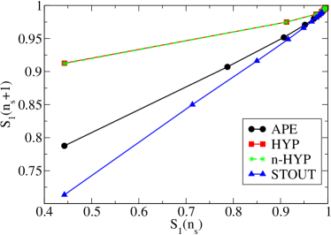
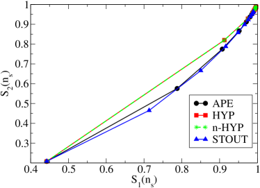
In MCRG the block spin transformation of an ensemble of spin configurations distributed according to an action leads to another ensemble with a different effective action , thus following a renormalized trajectory (connecting fixed points) in the space of coupling constants . We use this framework to study the change of the effective action under smearing transformations. The derivative matrix
| (5) |
(where the superscripts denote the number of blocking steps) defines a linearization of the flow in coupling space. It may be derived from cross-correlations of observables measured on configurations for different numbers of smearing steps [12],
| (6) | |||||
| (7) |
For BSTs close to a fixed point approaches the fixed point value and then its eigenvalues (if greater than 1) can be related to the relevant critical exponents through (here b is the scale factor of the BST).
In our case we are interested in for small . Its diagonalization gives the information about the main flow directions and the speed of flow. Actually, in case one knows the starting point in coupling space one can approximately recover . Related problems have been discussed recently in the context of trivializing maps [13]. For the gauge configuration ensembles used here we do not know , since they result from a simulation with dynamical fermions and thus the full effective gauge action is not the simple one used for the gauge part alone.
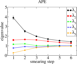
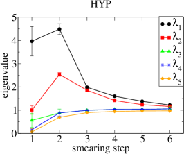
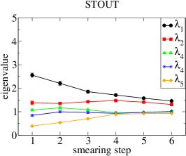
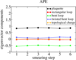
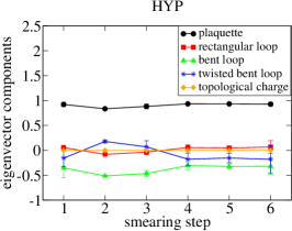
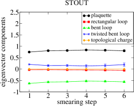
Figure 2 shows the leading eigenvalues of the diagonalization. Only two of them are significantly larger than 1; asymptotically they all approach 1 of course. The data for HYP smearing show a peak in the second step, they also give the largest eigenvalues indicating the strongest effect (on the observables considered).
Comparing the eigenvalues with the (normalized) eigenvectors for the leading eigenvalue (figure 3) we find that the dominant direction is the plaquette followed by the bent loop in all cases. The eigenvectors are defined only up to normalization (we normalized to unit length) and overall sign, which we choose such that continuity in is obtained.
The eigenvectors for the 2nd largest eigenvalue confirms that APE and STOUT smearing follow similar trajectories. Here the bent loop and the twisted bent loop dominate the flow. The eigenvectors for HYP smearing exhibit stronger fluctuation: more directions in coupling space are activated, mixing the local degrees of freedom stronger than the other types.
3 Conclusions
We try to make a step towards a systematic classification of gauge link smearing algorithms. Viewing smearing steps as analogues of block spin transformations, we attempt to quantify their effectiveness. This is a first attempt towards developing a tool for classification of the effect smearing has in configuration space. We find that the different methods follow similar trajectories in the space of local observables and effective couplings, however with different speed. The nHYP results are close to the HYP results. In our study only few local observables have been included; considering more would allow for a better and more complete quantification.
Acknowledgments:
We wish to thank G. Engel, C. Gattringer and A. Hasenfratz for discussions. The computations were done on the computing facilities of the computer center of Universität Graz.
References
- [1] APE Collaboration, M. Albanese et. al., Glueball masses and string tension in lattice QCD, Phys. Lett. B 192 (1987) 163.
- [2] F. D. R. Bonnet, D. B. Leinweber, A. G. Williams, and J. M. Zanotti, Improved smoothing algorithms for lattice gauge theory, Phys. Rev. D65 (2002) 114510, [hep-lat/0106023].
- [3] A. Hasenfratz and F. Knechtli, Flavor symmetry and the static potential with hypercubic blocking, Phys. Rev. D 64 (2001) 034504, [hep-lat/0103029].
- [4] A. Hasenfratz, R. Hoffmann and S. Schaefer,Hypercubic smeared links for dynamical fermions, JHEP 0705 (2007) 029, [hep-lat/0702028].
- [5] C. Morningstar and M. Peardon, Analytic smearing of SU(3) link variables in lattice QCD, Phys. Rev. D 69 (2004) 054501, [hep-lat/0311018].
- [6] S. Dürr, Gauge action improvement and smearing, Comput. Phys. Commun. 172 (2005) 163, [hep-lat/0409141].
- [7] C. Gattringer, A new approach to Ginsparg-Wilson fermions, Phys. Rev. D 63 (2001) 114501, [hep-lat/0003005].
- [8] C. Gattringer, I. Hip, and C. B. Lang, Approximate Ginsparg-Wilson fermions: A first test, Nucl. Phys. B 597 (2001) 451, [hep-lat/0007042].
- [9] C. Gattringer, C. Hagen, C. B. Lang, M. Limmer, D. Mohler, and A. Schäfer, Hadron spectroscopy with dynamical Chirally Improved fermions, Phys. Rev. D 79 (2009) 054501, [arXiv:0812.1681].
- [10] G. P. Engel, C. B. Lang, M. Limmer, D. Mohler, and A. Schäfer, Meson and baryon spectrum for QCD with two light dynamical quarks, Phys. Rev. D82 (2010) 034505, [arXiv:1005.1748].
- [11] S.-K. Ma, Renormalization group by Monte Carlo methods, Phys. Rev. Lett. 37 (1976) 461.
- [12] R. H. Swendsen, Monte Carlo renormalization group, Phys. Rev. Lett. 42 (1979) 859.
- [13] M. Lüscher, Trivializing maps, the Wilson flow and the HMC algorithm, Commun. Math. Phys. 293 (2010) 899, [arXiv:0907.5491].