Chemotaxis When Bacteria Remember: Drift versus Diffusion

Abstract

Escherichia coli (E. coli) bacteria govern their trajectories by switching between running and tumbling modes as a function of the nutrient concentration they experienced in the past. At short time one observes a drift of the bacterial population, while at long time one observes accumulation in high-nutrient regions. Recent work has viewed chemotaxis as a compromise between drift toward favorable regions and accumulation in favorable regions. A number of earlier studies assume that a bacterium resets its memory at tumbles – a fact not borne out by experiment – and make use of approximate coarse-grained descriptions. Here, we revisit the problem of chemotaxis without resorting to any memory resets. We find that when bacteria respond to the environment in a non-adaptive manner, chemotaxis is generally dominated by diffusion, whereas when bacteria respond in an adaptive manner, chemotaxis is dominated by a bias in the motion. In the adaptive case, favorable drift occurs together with favorable accumulation. We derive our results from detailed simulations and a variety of analytical arguments. In particular, we introduce a new coarse-grained description of chemotaxis as biased diffusion, and we discuss the way it departs from older coarse-grained descriptions.

Author Summary

The chemotaxis of Escherichia coli is a prototypical model of navigational strategy. The bacterium maneuvers by switching between near-straight motion, termed runs, and tumbles which reorient its direction. To reach regions of high nutrient concentration, the run-durations are modulated according to the nutrient concentration experienced in recent past. This navigational strategy is quite general, in that the mathematical description of these modulations also accounts for the active motility of C. elegans and for thermotaxis in Escherichia coli. Recent studies have pointed to a possible incompatibility between reaching regions of high nutrient concentration quickly and staying there at long times. We use numerical investigations and analytical arguments to reexamine navigational strategy in bacteria. We show that, by accounting properly for the full memory of the bacterium, this paradox is resolved. Our work clarifies the mechanism that underlies chemotaxis and indicates that chemotactic navigation in wild-type bacteria is controlled by drift while in some mutant bacteria it is controlled by a modulation of the diffusion. We also propose a new set of effective, large-scale equations which describe bacterial chemotactic navigation. Our description is significantly different from previous ones, as it results from a conceptually different coarse-graining procedure.

Introduction

The bacterium E. coli moves by switching between two types of motions, termed ‘run’ and ‘tumble’ bergbook . Each results from a distinct movement of the flagella. During a run, flagella motors rotate counter-clockwise (when looking at the bacteria from the back), inducing an almost constant forward velocity of about $20\mu m/s$, along a near-straight line. In an environment with uniform nutrient concentration, run durations are distributed exponentially with a mean value of about $\tau_{R}=1s$ berg72 . When motors turn clockwise, the bacterium undergoes a tumble, during which, to a good approximation, it does not translate but instead changes its direction randomly. In a uniform nutrient-concentration profile, the tumble duration is also distributed exponentially but with a much shorter mean value of about $\tau_{T}=0.1s$ turner .

When the nutrient (or, more generally, chemoattractant) concentration varies in space, bacteria tend to accumulate in regions of high concentration footnote ; adler . This is achieved through a modulation of the run durations. The biochemical pathway that controls flagella dynamics is well understood bergbook ; eisen ; leibler ; uri and the stochastic ‘algorithm’ which governs the behavior of a single motor is experimentally measured. The latter is routinely used as a model for the motion of a bacteria with many motors bergbook ; gennes ; kafri ; verg ; lars . This algorithm represents the motion of the bacterium as a non-Markovian random walker whose stochastic run durations are modulated via a memory kernel, shown in Fig. 1. Loosely speaking, the kernel compares the nutrient concentration experienced in the recent past with that experienced in the more distant past. If the difference is positive, the run duration is extended; if it is negative, the run duration is shortened.

Figure 1: Bilobe response function of wild-type E. coli used in the numerics in Fig. 3. For the sake of computational simplicity, we have used a discrete sampling of the experimental data presented in Ref. segall instead of working with the complete data set. This did not affect our conclusions.

In a complex medium bacterial navigation involves further complications; for example, interactions among the bacteria, and degradations or other dynamical variations in the chemical environment. These often give rise to interesting collective behavior such as pattern formation cates_pnas ; mittal . However, in an attempt to understand collective behavior, it is imperative to first have at hand a clear picture of the behavior of a single bacterium in an inhomogeneous chemical environment. We are concerned with this narrower question in the present work.

Recent theoretical studies of single-bacterium behavior have shown that a simple connection between the stochastic algorithm of motion and the average chemotactic response is far from obvious gennes ; lars ; kafri ; verg . In particular, it appeared that favorable chemotactic drift could not be reconciled with favorable accumulation at long times, and chemotaxis was viewed as resulting from a compromise between the two lars . The optimal nature of this compromise in bacterial chemotaxis was examined in Ref. verg . In various approximations, while the negative part of the response kernel was key to favorable accumulation in the steady state, it suppressed the drift velocity. Conversely, the positive part of the response kernel enhanced the drift velocity but reduced the magnitude of the chemotactic response in the steady state.

Here, we carry out a detailed study of the chemotactic behavior of a single bacterium in one dimension. We find that, for an ‘adaptive’ response kernel (i.e., when the positive and negative parts of the response kernel have equal weight such that the total area under the curve vanishes), there is no incompatibility between a strong steady-state chemotaxis and a large drift velocity. A strong steady-state chemotaxis occurs when the positive peak of the response kernel occurs at a time much smaller than $\tau_{R}$ and the negative peak at a time much larger than $\tau_{R}$, in line with experimental observation. Moreover, we obtain that the drift velocity is also large in this case. For a general ‘non-adaptive’ response kernel (i.e., when the area under the response kernel curve is non-vanishing), however, we find that a large drift velocity indeed opposes chemotaxis. Our calculations show that, in this case, a position-dependent diffusivity is responsible for chemotactic accumulation.

In order to explain our numerical results, we propose a simple coarse-grained model which describes the bacterium as a biased random walker with a drift velocity and diffusivity, both of which are, in general, position-dependent. This simple model yields good agreement with results of detailed simulations. We emphasize that our model is distinct from existing coarse-grained descriptions of E. coli chemotaxis schnitzer ; coarse ; mittal ; blythe . In these, coarse-graining was performed over left- and right-moving bacteria separately, after which the two resulting coarse-grained quantities were then added to obtain an equation for the total coarse-grained density. We point out why such approaches can fail and discuss the differences between earlier models and the present coarse-grained model.

Models

Following earlier studies of chemotaxis berg82 ; kafri , we model the navigational behavior of a bacterium by a stochastic law of motion with Poissonian run durations. A switch from run to tumble occurs during the small time interval between $t$ and $t+dt$ with a probability

$$\frac{dt}{\tau_{R}}\left\{1-\mathcal{F}\left[c\right]\right\}.$$ (1)

Here, $\tau_{R}\simeq 1s$ and $\mathcal{F}\left[c\right]$ is a functional of the chemical concentration, $c(t^{\prime})$, experienced by the bacterium at times $t^{\prime}\leq t$. In shallow nutrient gradients, the functional can be written as

$$\mathcal{F}\left[c\right]=\int_{-\infty}^{t}dt^{\prime}R(t-t^{\prime})c(t^{\prime})$$ (2)

The response kernel, $R(t)$, encodes the action of the biochemical machinery that processes input signals from the environment. Measurements of the change in the rotational bias of a flagellar motor in wild-type bacteria, in response to instantaneous chemoattractant pulses were reported in Refs. berg82 ; segall ; experiments were carried out with a tethering assay. The response kernel obtained from these measurements has a bimodal shape, with a positive peak around $t\simeq 0.5s$ and a negative peak around $t\simeq 1.5s$ (see Fig. 1). The negative lobe is shallower than the positive one and extends up to $t\simeq 4s$, beyond which it vanishes. The total area under the response curve is close to zero. As in other studies of E. coli chemotaxis, we take this response kernel to describe the modulation of run duration of swimming bacteria gennes ; lars ; kafri ; verg . Recent experiments suggest that tumble durations are not modulated by the chemical environment and that as long as tumbles last long enough to allow for the reorientation of the cell, bacteria can perform chemotaxis successfully bai ; mora .

The model defined by Eqs. 1 and 2 is linear. Early experiments pointed to a non-linear, in effect a threshold-linear, behavior of a bacterium in response to chemotactic inputs berg82 ; segall . In these studies, a bacterium modulated its motion in response to a positive chemoattractant gradient, but not to a negative one. In the language of present model, such a threshold-linear response entails replacing the functional defined in Eq. 2 by zero whenever the integral is negative. More recent experiments suggest a different picture, in which a non-linear response is expected only for a strong input signal whereas the response to weak chemoattractant gradient is well described by a linear relation shimizu . Here, we present an analysis of the linear model. For the sake of completeness, in Supporting Information, we present a discussion of models which include tumble modulations and a non-linear response kernel. Although recent experiments have ruled out the existence of both these effects in E.coli chemotaxis, in general such effects can be relevant to other systems with similar forms of the response function.

The shape of the response function hints to a simple mechanism for the bacterium to reach regions with high nutrient concentration. The bilobe kernel measures a temporal gradient of the nutrient concentration. According to Eq. 1, if the gradient is positive, runs are extended; if it is negative, runs are unmodulated. However, recent literature gennes ; lars ; kafri has pointed out that the connection between this simple picture and a detailed quantitative analysis is tenuous. For example, de Gennes used Eqs. 1 to calculate the chemotactic drift velocity of bacteria gennes . He found that a singular kernel, $R(t)=\alpha\delta(t-\Delta)$, where $\delta$ is a Dirac function and $\alpha$ a positive constant, lead to a mean velocity in the direction of increasing nutrient concentration even when bacteria are memoryless ($\Delta=0$). Moreover, any addition of a negative contribution to the response kernel, as seen in experiments (see Fig. 1), lowered the drift velocity. Other studies considered the steady-state density profile of bacteria in a container with closed walls, both in an approximation in which correlations between run durations and probability density were ignored lars and in an approximation in which the memory of the bacterium was reset at run-to-tumble switches kafri . Both these studies found that, in the steady state, a negative contribution to the response function was mandatory for bacteria to accumulate in regions of high nutrient concentration. These results seem to imply that the joint requirement of favorable transient drift and steady-state accumulation is problematic. The paradox was further complicated by the observation kafri that the steady-state single-bacterium probability density was sensitive to the precise shape of the kernel: when the negative part of the kernel was located far beyond $\tau_{R}$ it had little influence on the steady-state distribution lars . In fact, for kernels similar to the experimental one, model bacteria accumulated in regions with low nutrient concentration in the steady state kafri .

Results

Simulations and analytical treatment of chemotactic bacterial accumulation

In order to resolve these paradoxes and to better understand the mechanism that leads to favorable accumulation of bacteria, we perform careful numerical studies of bacterial motion in one dimension. In conformity with experimental observations berg82 ; segall , we do not make any assumption of memory reset at run-to-tumble switches.

We model a bacterium as a one-dimensional non-Markovian random walker. The walker can move either to the left or to the right with a fixed speed, $v$, or it can tumble at a given position before initiating a new run. In the main paper, we present results only for the case of instantaneous tumbling with $\tau_{T}=0$, while results for non-vanishing $\tau_{T}$ are discussed in Supporting Information. There, we verify that for an adaptive response kernel $\tau_{T}$ does not have any effect on the steady-state density profile. For a non-adaptive response kernel, the correction in the steady-state slope due to finite $\tau_{T}$ is small and proportional to $\tau_{T}/\tau_{R}$.

The run durations are Poissonian and the tumble probability is given by Eq. 1. The probability to change the run direction after a tumble is assumed to have a fixed value, $q$, which we treat as a parameter. The specific choice of the value of $q$ does not affect our broad conclusions. We find that, as long as $q\neq 0$, only certain detailed quantitative aspects of our numerical results depend on $q$. (See Supporting Information for details on this point.) We assume that bacteria are in a box of size $L$ with reflecting walls and that they do not interact among each other. We focus on the steady-state behavior of a population. Reflecting boundary conditions are a simplification of the actual behavior angelani ; galajda ; as long as the total ‘probability current’ (see discussion below) in the steady state vanishes, our results remain valid even if the walls are not reflecting.

As a way to probe chemotactic accumulation, we consider a linear concentration profile of nutrient: $c(x)=cx$. We work in a weak gradient limit, i.e., the value of $\alpha c$ is chosen to be sufficiently small to allow for a linear response. Throughout, we use $c=1/L$ in our numerics. From the linearity of the problem, results for a different attractant gradient, $k/L$, can be obtained from our results through a scaling factor $k$. In the linear reigme, we obtain a spatially linear steady-state distribution of individual bacterium positions, or, equivalently, a linear density profile of a bacterial population. Its slope, which we denote by $\beta$, is a measure of the strength of chemotaxis. A large slope indicates strong bacterial preference for regions with higher nutrient concentration. Conversely, a vanishing slope implies that bacteria are insensitive to the gradient of nutrient concentration and are equally likely to be anywhere along the line. We would like to understand the way in which the slope $\beta$ depends on the different time scales present in the system.

Results with non-adaptive response kernels

One particular advantage of a linear model is that a general problem can be solved by superposing the solutions of simpler problems—namely, with delta-function response kernels—with suitably chosen coefficients. Thus, solving the problem with a singular response kernel amounts to a full solution and we focus here on this case.

In our simulations, we start from an arbitrary bacterium position inside a box of size $L$. Each time step has a duration $dt$, during which a running bacterium moves over a distance $vdt$. This distance corresponds to one lattice spacing in our model, in which a lattice is introduced because time is discretized. Throughout the numerics, we use $dt=0.01s$ and $v=10\mu m/s$, which means that the lattice spacing in our simulations is $0.1\mu m$. Results for different values of $v$ can be obtained by rescaling the lattice spacing accordingly. At the end of each time step, we compute the functional defined in Eq. 2; for a singular response kernel, $R(t)=\alpha\delta(t-\Delta)$, this takes the form $\alpha c\left[x(t-\Delta)\right]$, where $c\left[x(t-\Delta)\right]$ is the nutrient concentration experienced by the bacterium at time $t-\Delta$. At the end of each time step the bacterium either tumbles, with a probability $\left(1-\alpha c\left[x(t-\Delta)\right]\right)dt/\tau_{R}$, or continues to move in the same direction. At every tumble, the velocity of the bacterium is reversed with a probability $q$.

The system reaches a steady state over a time scale which is of order $L^{2}/D$, where the diffusivity is given by $D=v^{2}\tau_{R}$. We verify numerically that after this time the bacterial density profile inside the box does not change further and assumes a time-independent linear form. We focus on the slope, $\beta$, of this profile. For an experimental realization of the steady-state behavior of a single bacterium, we provide here an estimate of the time scales and length scales involved. Since the long-time behavior of the system is diffusive (see the discussion of the coarse-grained model below), the relaxation time is $L^{2}/D$. Our results on the steady-state distribution of bacteria hold, realistically, if this relaxation time does not exceed the typical division time of an E. coli bacterium, which is of the order of $30$ minutes. Substituting experimental values for the parameters, we find the description should be valid for system sizes $L\lesssim 400\mu m$. In our simulations, we use a somewhat larger system ($L=1000\mu m$) so as to have cleaner results with negligible effects of the reflecting walls at the two boundaries. (Numerics data show that the width of the boundary layer is about $\sim 80\mu m$.)

According to our numerical simulations, for $\alpha<0$, $\beta$ increases with $\Delta$ and displays a plateau for $\Delta\gg\tau_{R}$ (Fig. 2). Simulations probing various values of $\tau_{R}$ also confirmed that $\beta=F(\Delta/\tau_{R})$, i.e., that the slope is a scaling function of $\Delta/\tau_{R}$. Clearly, for positive $\alpha$ the sign of $\beta$ is simply reversed, which corresponds to an unfavorable chemotaxis schnitzer ; lars .

Figure 2: The slope $\beta$ (scaled by a factor of $10^{8}$) as a function of $\Delta/\tau_{R}$, for the choice of response kernel $R(t)=\alpha\delta(t-\Delta)$. Note that for $\Delta\gg\tau_{R}$ the slope saturates to a non-vanishing value. The symbols $+$, $\ast$, and $\square$ correspond to slopes measured in simulations with $\tau_{R}=1.5,1.0$, and $0.5$ seconds, respectively. The black solid circles are derived from our coarse-grained formulation (Eq. 9). Here $q=0.5$, $\alpha=-0.02$, $L=1000\mu m$, $c=0.001\mu m^{-1}$, $v=10\mu m/s$.

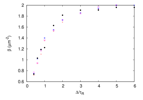
For small $\Delta$, one can write down an approximate master equation for left-mover and right-mover densities and use it to show that the slope increases linearly with $\Delta$ (see Supporting Information for details). It is surprising, however, that the slope appears to saturate to a non-vanishing value for $\Delta\gg\tau_{R}$. Indeed one would expect that, if the response kernel relies on a time much earlier than $t-\tau_{R}$, a large enough number of tumbles occur between this past time and the present time so as to eliminate any correlation between the nutrient concentration in the past and the present direction of motion. If this argument holds, one would expect that the slope $\beta$ vanish for $\Delta\gg\tau_{R}$. Below, we return to this argument and explain why it is misleading.

Results with adaptive response kernels

For wild-type bacteria, the total area under the response kernel vanishes (Fig. 1). As a result, their behavior is adaptive: chemotaxis is insensitive to the overall level of nutrient, but sensitive to spatial variations segall ; berg82 . In this section, before examining the case of a bilobe response kernel similar to the experimental one, we consider a toy model defined by the difference of two singular forms: $R(t)=\alpha\delta(t-\Delta_{1})-\alpha\delta(t-\Delta_{2})$, with $\alpha>0$. Because our problem is linear, the steady-state slope of bacterial density, $\beta$, can be calculated from a simple linear superposition, as:

$$\beta=F\left(\frac{\Delta_{1}}{\tau_{R}}\right)-F\left(\frac{\Delta_{2}}{\tau_{R}}\right).$$ (3)

Since the function $F(\cdot)$ is monotonic, the absolute value of $\beta$ increases with the difference of $\Delta_{1}$ and $\Delta_{2}$. Strong chemotaxis occurs when $\Delta_{1}=0$ and $\Delta_{2}\gg\tau_{R}$.

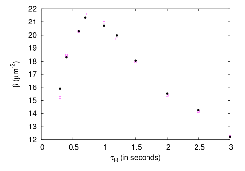
We now turn to the experimental case of a bilobe response kernel. It is not computationally feasible to work with the complete set of experimental data segall , so we have used a discrete subset (Fig. 1) which we represent as a series of delta-functions. Given this approximate response kernel, we investigate the behavior of the slope as a function of $\tau_{R}$. Based on our results for the case of two delta functions, we expect that chemotaxis be weak if $\tau_{R}$ is either much smaller than the delay of the positive peak in the response kernel or much larger than the delay of the negative peak. We expect optimum chemotaxis for a value of $\tau_{R}$ that falls in between the two delays. We verify this prediction in Fig. 3 (in the linear model). We note that the maximum slope occurs for a value of $\tau_{R}$ close to the experimentally recorded value of about $1s$.

Figure 3: The slope $\beta$ (scaled by a factor of $10^{8}$) as a function of $\tau_{R}$ for the experimental response kernel shown in Fig. 1. Open squares: numerical results from simulations. Solid circles: prediction of the coarse-grained model. Here, $q=0.4$, $L=1000\mu m$, $c=0.001\mu m^{-1}$, $v=10\mu m/s$.

Coarse-grained description of chemotaxis as diffusion with drift

In order to gain insight into our numerical results, we developed a simple coarse-grained model of chemotaxis. For the sake of simplicity, we first present the model for a non-adaptive, singular response kernel, $R(t)=\alpha\delta(t-\Delta)$, and, subsequently, we generalize the model to adaptive response kernels by making use of linear superposition.

The memory trace embodied by the response kernel induces temporal correlations in the trajectory of the bacterium. However, if we consider the coarse-grained motion of the bacterium over a spatial scale that exceeds the typical run stretch and a temporal scale that exceeds the typical run duration, then we can assume that it behaves as a Markovian random walker with drift velocity $V$ and diffusivity $D$. Since the steady-state probability distribution, $P(x)=P(\Delta,\tau_{R},x)$, is flat for $\alpha=0$, for small $\alpha$ we can write

$$P = P_{0}+\alpha{\mathcal{P}}(\Delta,\tau_{R},x)+o(\alpha^{2}),$$ (4)

$$D = D_{0}+\alpha{\mathcal{D}}(\Delta,\tau_{R},x)+o(\alpha^{2}),$$ (5)

$$V = \alpha{\cal V}(\Delta,\tau_{R},x)+o(\alpha^{2}).$$ (6)

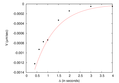
Here, $P_{0}=1/L$ and $D_{0}=v^{2}\tau_{R}$. Since we are neglecting all higher order corrections in $\alpha$, our analysis is valid only when $\alpha$ is sufficiently small. In particular, even when $\Delta\gg\tau_{R}$, we assume that the inequality $\Delta/\tau_{R}\ll 1/\alpha$ is still satisfied. The chemotactic drift velocity, $V$, vanishes if $\alpha=0$; it is defined as the mean displacement per unit time of a bacterium starting a new run at a given location. Clearly, even in the steady state when the current $J$, defined through $\partial_{t}P=-\partial_{x}J$, vanishes, $V$ may be non-vanishing (see Eq. 8 below). In general, the non-Markovian dynamics make $V$ dependent on the initial conditions. However, in the steady state this dependence is lost and $V$ can be calculated, for example, by performing a weighted average over the probability of histories of a bacterium. This is the quantity that is of interest to us. An earlier calculation by de Gennes showed that, if the memory preceding the last tumble is ignored, then for a linear profile of nutrient concentration the drift velocity is independent of position and takes the form $V=\alpha cv^{2}\tau_{R}\exp(-\Delta/\tau_{R})$ gennes . While the calculation applies strictly in a regime with $\Delta\ll\tau_{R}$ (because of memory erasure), in fact its result captures the behavior well over a wide range of parameters (see Fig. 4). To measure $V$ in our simulations, we compute the average displacement of the bacterium between two successive tumbles in the steady state, and we extract therefrom the drift velocity. (For details of the derivation, see Supporting Information.) We find that $V$ is negative for $\alpha<0$ and that its magnitude falls off with increasing values of $\Delta$ (Fig. 4). We also verify that $V$ indeed does not show any spatial dependence (data shown in Fig. $S3$ of Supporting Information). We recall that, in our numerical analysis, we have used a small value of $\alpha$; this results in a low value of $V$. We show below that for an experimentally measured bilobe response kernel, obtained by superposition of singular response kernels, the magnitude of $V$ becomes larger and comparable with experimental values.

Figure 4: The chemotactic drift velocity, $V$, as a function of $\Delta$, for the response kernel $R(t)=\alpha\delta(t-\Delta)$. Solid circles: numerical results. Line: approximate analytical results from gennes . $\tau_{R}=1s$ and other numerical parameters as in Fig. 2

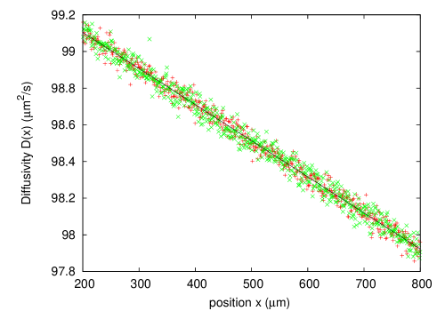
To obtain the diffusivity, $D$, we first calculate the effective mean free path in the coarse-grained model. The tumbling frequency of a bacterium is $(1-\alpha cx(t-\Delta))/\tau_{R}$ and depends on the details of its past trajectory. In the coarse-grained model, we replace the quantity $\alpha cx(t-\Delta)$ by an average $\alpha c\langle x(t-\Delta)\rangle$ over all the trajectories within the spatial resolution of the coarse-graining. Equivalently, in a population of non-interacting bacteria, the average is taken over all the bacteria contained inside a blob, and, hence, $\langle x(t-\Delta)\rangle$ denotes the position of the center of mass of the blob at a time $t-\Delta$ in the past. As mentioned above, the drift velocity is proportional to $\alpha$, so that $\alpha c\langle x(t-\Delta)\rangle=\alpha cx(t)+O(\alpha^{2})$. The average tumbling frequency then becomes $(1-\alpha cx))/\tau_{R}$ and, consequently, the mean free path becomes $\tau_{MFP}=\tau_{R}/(1-\alpha cx)\simeq\tau_{R}(1+\alpha cx)$. As a result, the diffusivity is expressed as $D=v^{2}\tau_{MFP}\simeq v^{2}\tau_{R}(1+\alpha cx)$. We checked this form against our numerical results (Fig. 5).

Figure 5: The diffusivity, $D(x)$, as a function of position, $x$, for the response kernel $R(t)=\alpha\delta(t-\Delta)$ with $\Delta=1s$ ($+$) and $2s$ ($\times$). Instead of plotting $D(x)$ for the entire range of $x$, we leave out boundary regions to avoid the effect of the reflecting walls. (From the numerics, the width of the boundary layer is $\sim 80\mu m$.) $D(x)$ falls off linearly with $x$ and is independent of $\Delta$. Data fitting yields $D(x)=99.5-0.00197x$ and the coarse-grained model predicts $D(x)=v^{2}\tau_{R}(1+\alpha cx)$. For the chosen set of parameters, $v^{2}\tau_{R}=100\mu m^{2}/s$ and the $v^{2}\tau_{R}\alpha c=-0.002$. The discrepancy between the numerical and the predicted slopes is due to higher-order corrections in $\alpha$, while discretization of space in simulations causes the slight mismatch in the constant term. $\tau_{R}=1s$ and other numerical parameters are as in Fig. 2.

Having evaluated the drift velocity, $V$, and the diffusivity, $D$, we now proceed to write down the continuity equation (for a more rigorous but less intuitive approach, see verg ). For a biased random walker on a lattice, with position-dependent hopping rates $d^{+}(x)$ and $d^{-}(x)$ towards the right and the left, respectively, one has $V=a\left(d^{+}(x)-d^{-}(x)\right)$ and $D=a^{2}\left(d^{+}(x)+d^{-}(x)\right)/2$, where $a$ is the lattice constant. In the continuum limit, the temporal evolution of the probability density is given by a probability current, as

$$\partial_{t}P=-\partial_{x}J,$$ (7)

where the current takes the form

$$J=VP-\partial_{x}\left(DP\right).$$ (8)

For reflecting boundary condition, $J=0$ in the steady state. This constraint yields a steady-state slope

$$\beta=\alpha\partial_{x}{\cal P}=\alpha\frac{P_{0}}{D_{0}}\left({\cal V}-\partial_{x}{\cal D}\right)=\frac{\alpha{\cal V}}{Lv^{2}\tau_{R}}-\frac{\alpha c}{L}$$ (9)

for small $\alpha$. We use our measured values for $V$ and $D$ (Figs. 4 and 5), and compute the slope using Eq. 9. (For details of the measurement of $V$, see Supporting Information.) We compare our analytical and numerical results in Fig. 2, which exhibits close agreement.

According to Eq. 9, steady-state chemotaxis results from a competition between drift motion and diffusion. For $\alpha<0$, the drift motion is directed toward regions with a lower nutrient concentration and hence opposes chemotaxis. Diffusion is spatially dependent and becomes small for large nutrient concentrations (again for $\alpha<0$), thus increasing the effective residence time of the bacteria in favorable regions. For large values of $\Delta$, the drift velocity vanishes and one has a strong chemotaxis as $\Delta$ increases (Fig. 2). Finally, for $\Delta=0$, the calculation by de Gennes yields $V=\alpha cv^{2}\tau_{R}$ which exactly cancels the spatial gradient of $D$ (to linear order in $\alpha$), and there is no accumulation gennes ; lars .

These conclusions are easily generalized to adaptive response functions. For $R(t)=\alpha\delta(t-\Delta_{1})-\alpha\delta(t-\Delta_{2})$, within the linear response regime, the effective drift velocity and diffusivity can be constructed by simple linear superposition: The drift velocity reads $V=\alpha{\cal V}(\Delta_{1})-\alpha{\cal V}(\Delta_{2})$. Interestingly, the spatial dependence of $D$ cancels out and $D=D_{0}=v^{2}\tau_{R}$. The resulting slope then depends on the drift only and is calculated as

$$\beta=\frac{\alpha}{Lv^{2}\tau_{R}}\left({\cal V}(\Delta_{1})-{\cal V}(\Delta_{2})\right).$$ (10)

In this case, the coarse-grained model is a simple biased random walker with constant diffusivity. For $\Delta_{1}<\Delta_{2}$ and $\alpha>0$, the net velocity, proportional to $\alpha\left({\cal V}(\Delta_{1})-{\cal V}(\Delta_{2})\right)$, is positive and gives rise to a favorable chemotactic response, according to which bacteria accumulate in regions with high food concentration. Moreover, the slope increases as the separation between $\Delta_{1}$ and $\Delta_{2}$ grows. We emphasize that there is no incompatibility between strong steady-state chemotaxis and large drift velocity. In fact, in the case of an adaptive response function, strong chemotaxis occurs only when the drift velocity is large.

For a bilobe response kernel, approximated by a superposition of many delta functions (Fig. 1), the slope, $\beta$, can be calculated similarly and in Fig. 3 we compare our calculation to the simulation results. We find close agreement in the case of a linear model with a bilobe response kernel and, in fact, also in the case of a non-linear model (see Supporting Information).

The experimental bilobe response kernel $R(t)$ is a smooth function, rather than a finite sum of singular kernels over a set of discrete $\Delta$ values (as in Fig. 1). Formally, we integrate singular kernels over a continuous range of $\Delta$ to obtain a smooth response kernel. If we then integrate the expression for the drift velocity obtained by de Gennes, according to this procedure, we find an overall drift velocity $V\sim 0.3\mu m/s$, for the concentration gradient considered ($\nabla c=0.001\mu m^{-1}$). By scaling up the concentration gradient by a factor of $\kappa$, the value of $V$ can also be scaled up by $\kappa$ and can easily account for the experimentally measured velocity range.

Discussion

We carried out a detailed analysis of steady-state bacterial chemotaxis in one dimension. The chemotactic performance in the case of a linear concentration profile of the chemoattractant, $c(x)=cx$, was measured as the slope of the bacterium probability density profile in the steady state. For a singular impulse response kernel, $R(t)=\alpha\delta(t-\Delta)$, the slope was a scaling function of $\Delta/\tau_{R}$, which vanished at the origin, increased monotonically, and saturated at large argument. To understand these results we proposed a simple coarse-grained model in which bacterial motion was described as a biased random walk with drift velocity, $V$, and diffusivity, $D$. We found that for small enough values of $\alpha$, $D$ was independent of $\Delta$ and varied linearly with nutrient concentration. By contrast, $V$ was spatially uniform and its value decreased monotonically with $\Delta$ and vanished for $\Delta\gg\tau_{R}$. We presented a simple formula for the steady-state slope in terms of $V$ and $D$. The prediction of our coarse-grained model agreed closely with our numerical results. Our description is valid when $\alpha$ is small enough, and all our results are derived to linear order in $\alpha$. We assume $\Delta/\tau_{R}\ll 1/\alpha$ is always satisfied.

Our results for an impulse response kernel can be easily generalized to the case of response kernels with arbitrary shapes in the linear model. For an adaptive response kernel, the spatial dependence of the diffusivity, $D$, cancels out but a positive drift velocity, $V$, ensures bacterial accumulation in regions with high nutrient concentration, in the steady state. In this case, the slope is directly proportional to the drift velocity. As the delay between the positive and negative peaks of the response kernel grows, the velocity increases, with consequent stronger chemotaxis.

Earlier studies of chemotaxis schnitzer ; coarse ; mittal ; blythe put forth a coarse-grained model different from ours. In the model first proposed by Schnitzer for a single chemotactic bacterium schnitzer , he argued that, in order to obtain favorable bacterial accumulation, tumbling rate and ballistic speed of a bacterium must both depend on the direction of its motion. In his case, the continuity equation reads

$$\partial_{t}P=\partial_{x}\left[\frac{\gamma_{L}v_{R}-\gamma_{R}v_{L}}{\gamma_{L}+\gamma_{R}}P-2\frac{v_{R}+v_{L}}{\gamma_{R}+\gamma_{L}}\partial_{x}\left(\frac{v_{R}v_{L}}{v_{R}+v_{L}}P\right)\right],$$ (11)

where $v_{L(R)}$ is the ballistic speed and $\gamma_{L(R)}$ is the tumbling frequency of a bacterium moving toward the left (right). For E. coli, as discussed above, $v_{L}=v_{R}=v$, a constant independent of the location. In that case, Eq. 11 predicts that in order to have a chemotactic response in the steady state, one must have a non-vanishing drift velocity, i.e., $\left(\gamma_{L}v_{R}-\gamma_{R}v_{L}\right)/(\gamma_{L}+\gamma_{R})\neq 0$. This contradicts our findings for non-adaptive response kernels, according to which a drift velocity only hinders the chemotactic response. The spatial variation of the diffusivity, instead, causes the chemotactic accumulation. This is not captured by Eq. 11. In the case of adaptive response kernels, the diffusivity becomes uniform while the drift velocity is positive, favoring chemotaxis. Comparing the expression of the flux, $J$, obtained from Eqs. 7 and 8 with that from Eq. 11, and matching the respective coefficients of $P$ and $\partial_{x}P$, we find $D=2v_{R}v_{L}/(\gamma_{R}+\gamma_{L})$ and $V=(\gamma_{L}v_{R}-\gamma_{R}v_{L})/(\gamma_{L}+\gamma_{R})$. As we argued above in discussing the coarse-grained model for adaptive response kernels, both $D$ and $V$ are spatially independent. This puts strict restrictions on the spatial dependence of $v_{L(R)}$ and $\gamma_{L(R)}$. For example, as in E. coli chemotaxis $v_{L}=v_{R}=v$, our coarse-grained description is recovered only if $\gamma_{L}$ and $\gamma_{R}$ are also independent of $x$.

We comment on a possible origin of the discrepancy between our work and earlier treatments. In Ref. schnitzer , a continuity equation was derived for the coarse-grained probability density of a bacterium, starting from a pair of approximate master equations for the probability density of a right-mover and a left-mover, respectively. As the original process is non-Markovian, one can expect a master equation approach to be valid only at scales that exceed the scale over which spatiotemporal correlations in the behavior of the bacterium are significant. In particular, a biased diffusion model can be viewed as legitimate only if the (coarse-grained) temporal resolution allows for multiple runs and tumbles. If so, at the resolution of the coarse-grained model, left- and right-movers become entangled, and it is not possible to perform a coarse-graining procedure on the two species separately. Thus one cannot define probability densities for a left- and a right-mover that evolves in a Markovian fashion. In our case, left- and right-movers are coarse-grained simultaneously, and the total probability density is Markovian. Thus, our diffusion model differs from that of Ref. schnitzer because it results from a different coarse-graining procedure. The model proposed in Ref. schnitzer has been used extensively to investigate collective behaviors of E. coli bacteria such as pattern formation coarse ; mittal ; blythe . It would be worth asking whether the new coarse-grained description can shed new light on bacterial collective behavior.

Supporting Information

Small-argument behavior of $F\left(\Delta/\tau_{R}\right)$

Here, we argue that for small $\Delta/\tau_{R}$ the function $F\left(\Delta/\tau_{R}\right)$ is linear. First, note that for an impulse response kernel, $R(t)=\alpha\delta(t-\Delta)$ the tumbling probability during the interval $[t,t+dt]$ is $\left[1-\alpha cx(t-\Delta)\right]dt/\tau_{R}$. For small $\Delta$, we can assume that no tumbling occurs during the interval $[t-\Delta,t]$. Then the effective tumbling rates become $\left[1-\alpha c(x-v\Delta)\right]/\tau_{R}$ for right-movers and $\left[1-\alpha c(x+v\Delta)\right]/\tau_{R}$ for left-movers. Based on this observation, we can write a pair of master equations that govern the densities of left-movers and right-movers, and we can solve them in the steady state. We obtain the slope, $\beta$, expressed as

$$\beta=-\frac{2\alpha c\Delta}{L\tau_{R}}.$$ (12)

Thus, in the limit $\Delta\ll\tau_{R}$ the scaling function $F(\Delta/\tau_{R})$ depends linearly on its argument.

Chemotactic drift velocity as a function of position

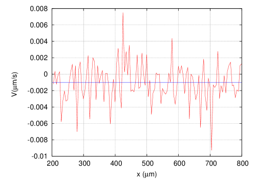
Here, we show a sample of our numerical results on the drift velocity $V$ as a function of position. We measure the average displacement of a bacterium in the steady state (see the corresponding discussion in the paper), and we compute $V$ therefrom. Specifically, we perform the following procedure. We denote by $m_{L}(x)$ and $m_{R}(x)$ the total number of leftward and rightward runs, respectively, that initiate at the position $x$, at a time $t$, for a population of non-interacting bacteria. These quantities are well-defined in the context of our numerics because space is discretized. Furthermore, let $S_{L}(x)$ and $S_{R}(x)$ be the total leftward and rightward displacement, respectively, of the bacteria that undergo these runs. The average displacement per run is then given by $[S_{R}(x)-S_{L}(x)]/[m_{R}(x)+m_{L}(x)]$. Of course, the choice of the time scale as the duration of a run is arbitrary and other choices are equally valid. To leading order, this average displacement is linear in $\alpha$. The drift velocity $V$, to order $\alpha$, is then obtained by dividing this average displacement by $\tau_{R}$. (Note that any $O(\alpha)$ correction to $\tau_{R}$ leads to $O(\alpha^{2})$ correction to $V$, which we ignore here.) We find that up to the noise present in our numerical measurement, $V$ does not display any dependence on position. An example is illustrated in Fig. 6.

Figure 6: Drift velocity, $V$, as a function of position, $x$, for the case of a singular response kernel $R(t)=\alpha\delta(t-\Delta)$ (red line). Instead of showing the plot for the entire range of $x$, we leave out boundary regions to discard the effect of the reflecting walls. Our numerics show that the width of the boundary layer is $\sim 80\mu m$. Here, $L=1000\mu m$, $q=1.0$, $\tau_{R}=1s$, $\Delta=1s$, $\tau_{T}=0$, $v=10\mu m/s$, $\alpha=-0.1$, $c=0.001{\mu m}^{-1}$. Based on the data shown, the drift velocity is $0.001\pm 0.0001\mu m/s$ (blue line).

Dependence of $V$ on the turning probability $q$

In our model, $q$ denotes the turning probability, i.e., the probability that the run direction inverses after a tumble. Our numerical explorations indicate that changing the value of $q$ does not affect the qualitative behavior of the system. However, the numerical value of the drift velocity, and the value of $\beta$ depend on $q$. In Fig. 7, we exhibit the variation of $V$ as a function of $q$, in the case of an adaptive response function.

Figure 7: The drift velocity, $V$, as a function of the turning probability, $q$, for the case of a singular adaptive response kernel $R(t)=\alpha\delta(t-\Delta_{1})-\alpha\delta(t-\Delta_{2})$. Here, $L=1000\mu m$, $\tau_{R}=1s$, $\Delta_{1}=0.5s$, $\Delta_{2}=1.5s$, $\tau_{T}=0$, $v=10\mu m/s$, $\alpha=0.1$, $c=0.001{\mu m}^{-1}$.

Results in the non-linear model

Some earlier experiments indicate that bacteria modulate their run durations in response to a positive concentration gradient, but not to a negative one. In order to incorporate this feature in our model, we have to go beyond the linear response regime. In the non-linear model, whenever the linear functional (Eq. 2) becomes negative, it is replaced by $0$. This is the only difference with the linear model. Thus, for a purely positive response kernel the non-linear model behaves identically to the linear model, while for a purely negative response kernel the non-linear model displays no chemotaxis whatsoever. Hereafter, we examine only adaptive response kernels with balanced positive and negative contributions.

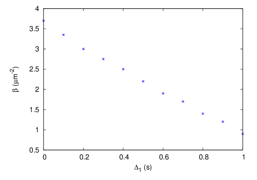
We first consider the idealized response kernel made of the superposition of positive and negative delta functions, $R(t)=\alpha\delta(t-\Delta_{1})-\alpha\delta(t-\Delta_{2})$. Simulations show that many qualitative features of the linear model still hold in the non-linear model. The scaling form valid in the linear case breaks down in the non-linear case, but the slope $\beta$ increases with the separation between $\Delta_{1}$ and $\Delta_{2}$ and ultimately saturates to a non-vanishing value. Figures 8 and 9 display results of simulations. As expected, strong chemotaxis occurs when $\Delta_{1}=0$ and $\Delta_{2}$ is substantially larger than $\tau_{R}$. We have also verified that tumbling does not have much of an effect on the slope.

Figure 8: The slope, $\beta$ (scaled by a factor of $10^{8}$), as a function of $\Delta_{2}$, for $\Delta_{1}=0.5s$, in a non-linear model with balanced response kernel, $R(t)=\alpha\delta(t-\Delta_{1})-\alpha\delta(t-\Delta_{2})$. As in the linear model, $\beta$ increases with the difference of $\Delta_{1}$ and $\Delta_{2}$. Here, $\tau_{R}=1$ sec, $q=0.4$, $\alpha=0.1$, $L=1000\mu m$, $c=0.001\mu m^{-1}$, $v=10\mu m/s$.

Figure 9: The slope, $\beta$ (scaled by a factor of $10^{8}$), as a function of $\Delta_{1}$, for $\Delta_{2}=1.5s$, in a non-linear model with balanced response kernel, $R(t)=\alpha\delta(t-\Delta_{1})-\alpha\delta(t-\Delta_{2})$. Numerical parameters are as in Fig. 8.

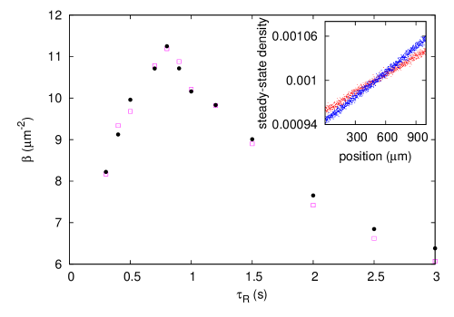
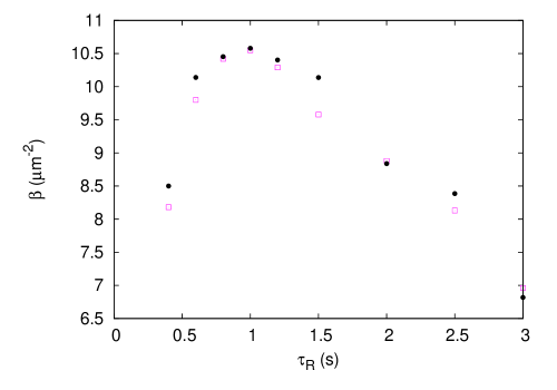
In the experimental case of a bilobe response kernel (Fig. 1 in the paper), we find that strong chemotaxis occurs when $\tau_{R}$ lies between the positive and the negative peaks of the response kernel, as found in the linear case. For smaller or larger values of $\tau_{R}$, chemotaxis becomes weak. Figures 10 and 11 show our numerical results for $q=0.4$ and $q=0.5$, respectively. We note that, in both plots the value of $\tau_{R}$ for which the slope is maximum falls close to the experimental value of about $1s$. However, the exact position of the maximum depends on $q$. For $q=0.4$ (Fig.10) maximum occurs at $\tau_{R}\simeq 0.8s$, while for $q=0.5$ (Fig. 11) the maximum occurs at $\tau_{R}\simeq 1s$.

Figure 10: The slope, $\beta$ (scaled by a factor of $10^{8}$), as a function of $\tau_{R}$, in a non-linear model with the experimental bilobe response kernel of Fig. $1$ in the paper. Open squares: numerical results from simulations. Solid circles: prediction of the coarse-grained model. Numerical parameters as in Fig. $3$ in the paper. The inset shows the steady-state density profiles of the bacterial population for $\tau_{R}=0.3,0.8s$ (red and blue curve), respectively.

Figure 11: The slope, $\beta$ (scaled by a factor of $10^{8}$), as a function of $\tau_{R}$, in a non-linear model with the experimental bilobe response kernel of Fig. $1$ in the paper. Here, $q=0.5$ and the other numerical parameters are as in Fig. $3$ in the paper. Comparison with Fig. 10 shows that the position of the maximum depends on the value of $q$. Open squares: numerical results from simulations. Solid circles: prediction of the coarse-grained model.

Chemotaxis with non-vanishing tumbling durations

During a tumbling event the bacterium rotates about itself in a random fashion without any significant displacement. In a homogeneous nutrient concentration the average tumbling duration is $0.1s$, which is much smaller than the average run duration of $1s$. In the steady state one therefore expects that the bacterium spends only a fraction $\tau_{T}/\tau_{R}\simeq 0.1$ of the time in the tumbling state. For this reason, studies of chemotaxis often assume instantaneous tumbling.

It was shown recently that the existence of non-vanishing tumbling duration can yield interesting results: even with a punctual response kernel, $R(t)=\alpha\delta(t-\Delta)$ with $\Delta=0$, i.e. a memoryless bacterium, one can observe a chemotactic response (Kafri et al., 2008). Here, we provide a simplified derivation of the steady-state density profile in this Markovian limit. The result will prove useful also for the analysis of the non-Markovian case with $\Delta\neq 0$.

Let $L(x,t)$ and $R(x,t)$ be the density of left-movers and right-movers, respectively, at location $x$ and time $t$. We denote by $T^{R}(x,t)$ and $T^{L}(x,t)$ the densities of tumblers that were moving to the right and left, respectively, before tumbling. For $\Delta=0$, the time evolution of these quantities can be described by master equations. In the case in which tumble durations are not modulated and tumble-to-run switches always occur at a fixed rate $1/\tau_{T}$, the master equations read

$$\frac{\partial R(x,t)}{\partial t}= -v\partial_{x}R(x,t)+T^{R}(x,t)\frac{(1-q)}{\tau_{T}}$$ (13)

$$+T^{L}(x,t)\frac{q}{\tau_{T}}-R(x,t)\frac{1-\alpha cx}{\tau_{0}},$$

$$\frac{\partial L(x,t)}{\partial t}= v\partial_{x}L(x,t)+T^{L}(x,t)\frac{(1-q)}{\tau_{T}}$$ (14)

$$+T^{R}(x,t)\frac{q}{\tau_{T}}-L(x,t)\frac{1-\alpha cx}{\tau_{0}},$$

$$\frac{\partial T^{R}(x,t)}{\partial t}= R(x,t)\frac{1-\alpha cx}{\tau_{0}}-T^{R}(x,t)\frac{1}{\tau_{T}},$$ (15)

$$\frac{\partial T^{L}(x,t)}{\partial t}= L(x,t)\frac{1-\alpha cx}{\tau_{0}}-T^{L}(x,t)\frac{1}{\tau_{T}}.$$ (16)

We consider perfectly reflecting boundary conditions at $x=0$ and $x=L$. This implies that, in the steady state, we must have $R(x)=L(x)$. The steady-state (total) density at location $x$ then becomes

$$N(x)= R(x)+L(x)+T^{R}(x)+T^{L}(x)$$

$$= \frac{2}{L}\frac{1}{2+\frac{\tau_{T}}{\tau_{0}}(2-\alpha)}\left(1+\frac{\tau_{T}}{\tau_{0}}(1-\alpha cx)\right).$$ (17)

Therefore, the slope of the steady-state density profile is given by

$$\beta=G\left(\frac{\tau_{T}}{\tau_{0}}\right)=-2\alpha c\frac{1}{L}\frac{\tau_{T}}{\tau_{0}}\frac{1}{2+\frac{\tau_{T}}{\tau_{0}}(2-\alpha)}.$$ (18)

In Fig. 12, we compare this result with the slope measured in simulations. This plot demonstrates that, even in the absence of any memory or modulation of tumbling durations, it is possible to obtain chemotaxis in the steady state.

Figure 12: The steady-state slope $\beta$ as a function of $\tau_{T}/\tau_{0}$ for $\Delta=0$ and unmodulated tumbling. The solid line corresponds to the exact result from Eq. 18. Here we have used $L=1000\mu m$, $\alpha=-0.1$, $q=0.4$, $c=0.001\mu m^{-1}$, $v=10\mu m/sec$.

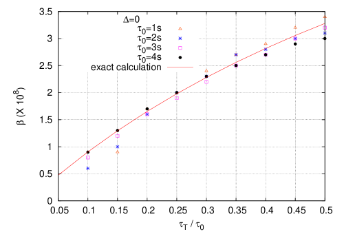
This result for the slope is slightly different for the case in which tumbling durations are modulated: then, $\tau_{T}$ in the above master equations is replaced by $\tau_{T}/(1+\alpha cx)$. Solving for the steady state, we find a total density

$$N(x)= R(x)+L(x)+T^{R}(x)+T^{L}(x)$$

$$= \frac{1}{L\left(1+\frac{\tau_{T}}{\tau_{0}}\right)}\left(1+\frac{\tau_{T}}{\tau_{0}}\frac{1-\alpha cx}{1+\alpha cx}\right).$$ (19)

For $\alpha cx\ll 1$, this is approximated by a linear form and the slope becomes

$$\beta=G\left(\frac{\tau_{T}}{\tau_{0}}\right)=-\frac{2\alpha c}{L}\frac{\tau_{T}}{\tau_{0}}\frac{1}{1+\frac{\tau_{T}}{\tau_{0}}(1-\alpha)}.$$ (20)

We compare this analytical result with simulations in Fig. 13, which shows a systematic deviation for large argument. We have verified that this mismatch originates in the linearizing approximation step from Eq. 19 to Eq. 20.

Figure 13: The slope, $\beta$, as a function of $\tau_{T}/\tau_{R}$ for $\Delta=0$ and modulated tumbling. Simulation parameters are $L=1000\mu m$, $\alpha=-0.1$, $q=0.4$, $c=0.001\mu m^{-1}$, $v=10\mu m/s$.

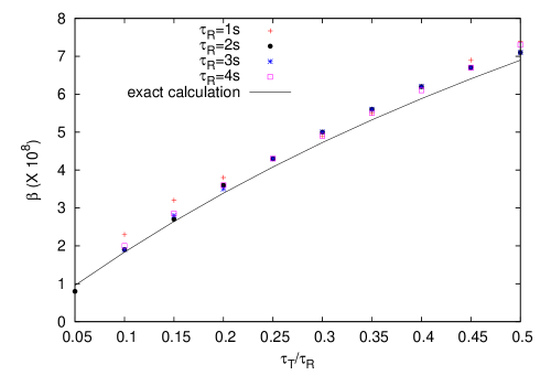
For $\Delta\neq 0$ and when both runs and tumbles are modulated, we measure the density profile in numerical simulations. For $R(t)=\alpha\delta(t-\Delta)$, our numerics indicate that the steady-state slope, $\beta$, is a sum of the Markovian component, $G$, defined in Eq. 20, and a non-Markovian component, $F$, which depends on $\Delta/\tau_{R}$ but is independent of $\tau_{T}$:

$$\beta=F\left(\frac{\Delta}{\tau_{R}}\right)+G\left(\frac{\tau_{T}}{\tau_{R}}\right).$$ (21)

In Fig. 14, we exhibit this scaling form as a function of $\tau_{T}/\tau_{R}$ for a fixed, non-vanishing value of $\Delta/\tau_{R}$. Our results suggests that $\beta$ is made up of two contributions: one from the modulating runs, encoded in $F$, and one from non-instantaneous tumbles, encoded in $G$. The latter contribution is independent of $\Delta$.

Figure 14: The scaling collapse of the slope, $\beta$, as a function of $\tau_{T}/\tau_{R}$ for fixed value of $\Delta/\tau_{R}$. We have used $\Delta/\tau_{R}=0.5$ here. The other simulation parameters are as in Fig. 13. We also plot the slope, $\beta$, in the non-linear model with $R(t)=\alpha\left[\delta(t-\Delta_{1})-\delta(t-\Delta_{2})\right]$, $\Delta_{1}=0s$ and $\Delta_{2}=1.5s$ and $\tau_{R}=1s$: $\beta$ does not show any significant dependence on $\tau_{T}$.

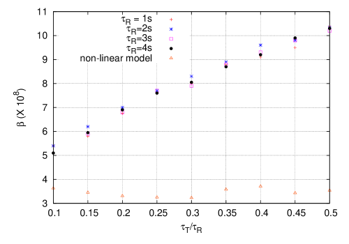
Finally, we can infer more general results from the simple form in Eq. 21. In particular, for an adaptive response function in the linear model, the positive and negative parts of the response function cancel out the effect of non-vanishing tumble durations. In this case, the steady-state slope, $\beta$, becomes independent of $\tau_{T}$. Interestingly, we find the same applies even in the non-linear model (see Fig. 14).

References

- (1) Berg HC (2003) E. coli in Motion (Springer-Verlag, New York).
- (2) Berg HC, Brown DA (1972) Chemotaxis in Eschericia coli analysed by three-dimensional tracking. Nature 239:500-504.
- (3) Turner L, Ryu WS, Berg HC (2000) Real-time imaging of fluorescent flagellar filaments. J Bacteriol 182:2793-2801.
- (4) The bacteria can also be repelled by chemorepellants and tend to accumulate in low chemical concentration. It is straightforward to reinterprete all our results and discussions for this case.
- (5) Adler J (1973) A method for measuring chemotaxis and use of the method to determine optimum conditions for chemotaxis by Escherichia coli. J Gen Microbiol 74:77-91.
- (6) Eisenbach M (1996) Control of bacterial chemotaxis. Mol Microbiol 20:903-910.
- (7) Barkai N, Leibler S (1997) Robustness in simple biochemical networds. Nature 387:913-917.
- (8) Alon U, Surette MG, Barkai N, Leibler S (1999) Robustness in bacterial chemotaxis. Nature 397:168-171.
- (9) de Gennes PG (2004) Chemotaxis and the role of internal delays. Eur Biophys J 33:691-693.
- (10) Kafri Y, da Silveira RA (2008) Steady-state chemotactic response in E. coli. Phys Rev Lett 100:238101-238105.
- (11) Celani A, Vergassola M (2010) Bacterial strategies for chemotaxis response. Proc Natl Acad Sci USA 107:1391-1396.
- (12) Clark DA, Grant LC (2005) The bacterial chemotaxis response reflects a compromise between transient and steady-state behavior. Proc Natl Acad Sci USA 102:9150-9155.
- (13) Cates ME, Marenduzzo D, Pagonabarraga I, Tailleur J (2010) Arrested phase separation in reproducing bacteria creates a generic route to pattern formation. Proc Natl Acad Sci USA 107:11715-11720.
- (14) Mittal N, Budrene EO, Brenner MP, van Oudenaarden A (2003) Motility of Escherichia coli cells in clusters formed by chemotactic aggregation. Proc Natl Acad Sci USA 100:13259-13263.
- (15) Schnitzer MJ (1993) Theory of continuum random walker and application to chemotaxis. Phys Rev E 48:2553-2568.
- (16) Tailleur J, Cates ME (2008) Statistical mechanics of interacting run-and-tumble bacteria. Phys Rev Lett 100:218103.
- (17) Thompson AG, Tailleur J, Cates ME, Blythe RA (2011) Lattice models of nonequilibrium bacterial dynamics. J Stat Mech P02029.
- (18) Block SM, Segall JE, Berg HC (1982) Impulse responses in bacterial chemotaxis. Cell 31:215-226.
- (19) Segall JE, Block SM, Berg HC (1986) Temporal comparisons in bacterial chemotaxis. Proc Natl Acad Sci USA 83:8987-8991.
- (20) Bai F, Branch RW, Nicolau Jr DV, Pilizota T, Steel BC, Maini PK, Berry RM (2010) Conformational spread as a mechanism for cooperativity in the bacterial flagellar switch. Science 327:685-689.
- (21) Mora T, Bai F, Che Y-S, Minamino T, Namba K, Wingreen NS (2011) Non-genetic individuality in Escherichia coli motor switching. Phys Biol 8:024001-024004.
- (22) Shimizu TS, Tu Y, Berg HC (2010) A modular gradient-sensing network for chemotaxis in Escherichia coli revealed by responses to time-varying stimuli. Mol Syst Biol 6:382-396.
- (23) Angelani L, Di Leonardo R, Ruocco G (2009) Self-Starting Micromotors in a Bacterial Bath. Phys Rev Lett 102:048104.
- (24) Galajda P, Keymer J, Chaikin P, Austin R (2007) A Wall of Funnels Concentrates Swimming Bacteria. J Bacteriol 189:8704-8707.