Distributed $k$-Core Decomposition

Abstract

Among the novel metrics used to study the relative importance of nodes in complex networks, $k$-core decomposition has found a number of applications in areas as diverse as sociology, proteinomics, graph visualization, and distributed system analysis and design. This paper proposes new distributed algorithms for the computation of the $k$-core decomposition of a network, with the purpose of (i) enabling the run-time computation of $k$-cores in “live” distributed systems and (ii) allowing the decomposition, over a set of connected machines, of very large graphs, that cannot be hosted in a single machine. Lower bounds on the algorithms complexity are given, and an exhaustive experimental analysis on real-world graphs is provided.

1 Introduction

In the last few years, a number of metrics and methods have been introduced for studying the relative “importance” of nodes within complex network structures. Examples include betweenness, eigenvector and closeness centrality indexes [5, 10]. Such studies have been applied in a variety of settings, including real networks like the Internet topology, social networks like co-authorships graphs, protein networks in bio-informatics, and so on.

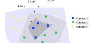
Figure 1: $k$–core decomposition for a sample graph.

Among these metrics, $k$-core decomposition is a well-established method for identifying particular subsets of the graph called $k$-cores, or $k$-shells [12]. Informally, a $k$-core is obtained by recursively removing all nodes of degree smaller than $k$, until the degree of all remaining vertices is larger than or equal to $k$. Nodes are said to have coreness $k$ (or, equivalently, to belong to the $k$-shell) if they belong to the $k$-core but not to the $(k+1)$-core. As an example of $k$-core decomposition for a sample graph, consider Figure 1. Note that by definition cores are “concentric”, meaning that nodes belonging to the 3-core belong to the 2-core and 1-core, as well. Larger values of “coreness”, though, clearly correspond to nodes with a more central position in the network structure.

$k$-core decomposition has found a number of applications; for example, it has been used to characterize social networks [12], to help in the visualization of complex graphs [1], to determine the role of proteins in complex proteinomic networks [2], and finally to identify nodes with good “spreading” properties in epidemiological studies [8].

Centralized algorithms for the $k$-core decomposition already exist [3]. Here, we consider the distributed version of this problem, which is motivated by the following scenarios:

• One-to-one scenario: The graph to be analyzed could be a “live” distributed system, such as a P2P overlay, that needs to inspect itself; one host is also one node in the graph, and connections among hosts are the edges. Given that cores with larger $k$ are known to be good spreaders [8], this information could be used at run-time to optimize the diffusion of messages in epidemic protocols [11].

• One-to-many scenario: The graph could be so large to not fit into a single host, due to memory restrictions; or its description could be inherently distributed over a collection of hosts, making it inconvenient to move each portion to a central site. So, one host stores many nodes and their edges. As an example, consider the Facebook social graph, with 500 million users (nodes) and more than 65 billion friend connections (edges) in December 2010; or the web crawls of Google and Yahoo, which stopped to announce the size of their indexes in 2005, when they both surpassed the 10 billion pages (nodes) milestone.

Interesting enough, the two scenarios turn out to be related: the former can be seen as a special case of the “inherent distribution” of the latter taken to its extreme consequences, with each host storing only one node and its edges.

The contribution of this paper is a novel algorithm that could be adapted to both scenarios. Reversing the above reasoning, Section 3 first proposes a version that can be applied to the one-to-one scenario, and then shows how to migrate it to the one-to-many scenario, by efficiently putting a collection of nodes under the responsibility of a single host. We prove that the resulting algorithm completes the $k$-core decomposition in $O(N)$ rounds, with $N$ being the number of nodes; more precisely, Section 4 shows an upper bound equal to $N-K+1$, with $K$ being the number of nodes with minimal degree, and describes a worst-case graph that requires exactly such number of rounds. While such upper bounds are rather high, real world graphs such as the Slashdot comment network, the citation graph of Arxiv or the Gnutella overlay network require a surprisingly low number of rounds, as demonstrated in the experiments described in Section 5.

2 Notation and system model

Given an undirected graph $G=(V,E)$ with $N=|V|$ nodes and $M=|E|$ edges, we define the concept of $k$–core decomposition:

Definition 1.

A subgraph $G(C)$ induced by the set $C\subseteq V$ is a k-core if and only if $\forall u\in C:\textit{d}_{G(C)}(u)\geq k$, and $G(C)$ is the maximum subgraph with this property.

Definition 2.

A node in $G$ is said to have coreness $k$ if and only if it belongs to the $k$-core but not the $(k+1)$-core.

Here, $\textit{d}_{G}(u)$ and $\textit{k}_{G}(u)$ denote the degree and the coreness of $u$ in $G$, respectively; in what follows, $G$ can be dropped when it is clear from the context. $G(C)=(C,E|C)$ is the subgraph of $G$ induced by $C$, where $E|C=\{(u,v)\in E:u,v\in C\}$.

The distributed system is composed by a collection of hosts $H$, whose overall goal is to compute the $k$-core decomposition of $G$. Each node $u$ is associated to exactly one host $h(u)\in H$, that is responsible for computing the coreness of $u$. Each host $x$ is thus responsible for a collection of nodes $V(x)$, defined as follows:

$$V(x)=\{u:h(u)=x\}.$$

Each host $x$ has access to two functions, $\textsl{neighbor}_{V}()$ and $\textsl{neighbor}_{H}()$, that return a set of neighbor nodes and neighbor hosts, respectively. Host $x$ may apply these functions to either itself or to the nodes under its responsibility; it cannot obtain information about neighbors of other hosts or nodes under the responsibility of other nodes. Formally, the functions are defined as follows:

$$\forall u\in V:\textsl{neighbor}_{V}(u) =\{v:(u,v)\in E\}$$

$$\forall x\in H:\textsl{neighbor}_{V}(x) =\{v:(u,v)\in E\wedge u\in V(x)\}$$

$$\forall x\in H:\textsl{neighbor}_{H}(x) =\{y:(u,v)\in E\wedge u\in V(x)\wedge v\in V(y)\}$$

A special case occurs when the graph to be analyzed coincides with the distributed system, i.e. $H=V$. When this happens, the label $u$ will be used to denote both the node and the host, and in general we will use the terms node and host interchangeably. Also, note that in this case $\textsl{neighbor}_{V}(u)$ = $\textsl{neighbor}_{H}(u)$.

Hosts communicate through reliable channels. For the duration of the computation, we assume that hosts do not crash.

3 Algorithm

Our distributed algorithm is based on the property of locality of the $k$-core decomposition: due to the maximality of cores, the coreness of node $u$ is the largest value $k$ such that $u$ has at least $k$ neighbors that belong to a $k$-core or a larger core. More formally,

Theorem 1 (Locality).

For each $u\in V$, $\textit{k}(u)=k$ if and only if

(i) there exist a subset $V_{k}\subseteq\textsl{neighbor}_{V}(u)$ such that $|V_{k}|=k$ and $\forall v\in V_{k}:\textit{k}(v)\geq k$;

(ii) there is no subset $V_{k+1}\subseteq\textsl{neighbor}_{V}(u)$ such that $|V_{k+1}|=k+1$ and $\forall v\in V_{k+1}:\textit{k}(v)\geq k+1$.

Proof

• Since $\textit{k}(u)=k$ there exists a (maximal) set $W_{k}\subseteq V$ such that $u\in W_{k}$ and $G(W_{k})$ is a $k$-core, and there is no set $W_{k+1}\subseteq V$ such that $u\in W_{k+1}$ and $G(W_{k+1})$ is a $(k+1)$-core. Indeed, $G(W_{k})$ is a $k$-core for all nodes in $W_{k}$, and so it is for at least $k$ neighbors of $u$, because of maximality. Part (ii) follows by contradiction: assume that $v_{1},\ldots,v_{k+1}$ are $k+1$ neighbors of $u$ that have coreness $k+1$ or more. Denote $W_{1},\ldots,W_{k+1}$ the subsets of nodes inducing their corresponding $(k+1)$-cores. Consider the set $U=\{u\}\cup\bigcup_{i=1}^{k+1}W_{i}$, that merges $u$ with all the $W_{i}$ sets. The subgraph $G(U)$ induced by $U$ contains at least $k+1$ nodes (because each $W_{i}$ contains at least $k+1$ nodes); for each node $v\in U$, $\textit{d}_{G(U)}(v)\geq k+1$, because $U$ is the union of $k+1$ $(k+1)$-cores and the $k+1$ neighbors of $u$ are included in it. But this proves that a $(k+1)$-core exists ($G(U)$ may well not be maximal) and $u$ belongs to it. Contradiction.

• For each node $v_{i}\in V_{k}$, $1\leq i\leq k$, $\textit{k}(v_{i})=k$ implies the existence of a set $W_{i}\subseteq V$ such that $G(W_{i})$ is a $k$-core of $G$ and $v_{i}\in W_{i}$. Consider the set $U=\{u\}\cup\bigcup_{i=1}^{k}W_{i}$. The subgraph $G(U)$ induced by $U$ contains at least $k+1$ nodes (because each $W_{i}$ contains at least $k+1$ nodes); for each node $v\in U$, $\textit{d}_{G(U)}(v)\geq k+1$, because it is the union of $k$ $k$-cores and the $k$ neighbors of $u$ are included in $U$. Thus, because of maximality, $G(U)$ is a $k$-core of $G$ containing $u$. Suppose now that there exists a subset $W\subseteq V$ such that $G(W)$ is a $(k+1)$-core containing $u$; this means that $u$ has at least $k+1$ neighbors, each of them with coreness $k+1$ or more; but this contradicts our hypothesis (ii). We can conclude that $\textit{k}(v)=k$.∎

The locality property tells us that the information about the coreness of the neighbors of a node is sufficient to compute its own coreness. Based on this idea, our algorithm works as follows: each node produces an estimate of its own coreness and communicates it to its neighbors; at the same time, it receives estimates from its neighbors and use them to recompute its own estimate; in the case of a change, the new value is sent to the neighbors and the process goes on until convergence.

This outline must be formalized in a real algorithm; we do it twice, for both the one-to-one and the one-to-many scenarios. We conclude the section with a few ideas about termination detection, that are valid for both versions.

3.1 One host, one node

Each node $u$ maintains the following variables:

• core is an integer that represents the local estimate of the coreness of $u$; it is initialized with the local degree.

• $\textsl{est}[\,]$ is an integer array containing one element for each neighbor; $\textsl{est}[v]$ represents the most up-to-date estimate of the coreness of $v$ known by $u$. In the absence of more precise information, all its entries are initialized to $+\infty$.

• changed is a Boolean flag set to true if core has been recently modified; initially set to false.

The protocol is described in Algorithm 1. Each node $u$ starts by broadcasting a message $\langle u,\textit{d}(u)\rangle$ containing its identifier and degree to all its neighbors. Whenever $u$ receives a message $\langle v,k\rangle$ such that $k<\textsl{est}[v]$, the entry $\textsl{est}[v]$ is updated with the new value. A new temporary estimate $t$ is computed by function computeIndex() in Algorithm 2. If $t$ is smaller than the previously known value of core, core is modified and the changed flag is set to true. Function computeIndex() returns the largest value $i$ such that there are at least $i$ entries equal or larger than $i$ in est, computed as follows: the first three loops compute how many nodes have estimate $i$ or more, $1\leq i\leq k$, and store this value in array count. The while loop searches the largest value $i$ such that $\textsl{count}[i]\geq i$, starting from $k$ and going down to $1$.

The protocol execution is divided in periodic rounds: every $\delta$ time units, variable changed is checked; if the local estimate has been modified, the new value is sent to all the neighbors and changed is set back to false. This periodic behavior is used to avoid flooding the system with a flow of estimate messages that are immediately superseded by the following ones.

It is worth remarking that during the execution, variable core at node $u$ (i) is always larger or equal than the real coreness value of $u$, and (ii) cannot increase upon the receipt of an update message. Informally, these two observations are the basis of the correctness proof contained in Section 4.

3.1.1 Example

We describe here a run of the algorithm on the simple sample graph reported in Fig. 2. At the first round, all nodes $v$ have $\textsl{core}=\textit{d}(v)$; nodes $2,3,4$ and $5$ send the same value $\textsl{core}=3$ with their neighbors: these messages do not cause any change in the estimates of the coreness of receiving nodes. However, in the same round, nodes $1$ and $6$ notify their $\textsl{core}=1$ value to nodes $2$ and $5$, respectively: as a consequence, node $2$ and $5$ update their estimates to $\textsl{core}=2$. Thus, in the second round another message exchange occurs, since nodes $2$ and $5$ notify their neighbors that their local estimate changed, i.e., they send $\textsl{core}=2$ to nodes $1,3,4$ and $3,4,6$, respectively. This causes an update $\textsl{core}=2$ at nodes $3$ and $4$, which have to send out another update $\textsl{core}=2$ to nodes $2$ and $4$ and nodes $3$ and $5$, respectively, in the third round. However, no local estimate changes from now on, which in turns means that the algorithm converged. Finally, $\textsl{core}=2$ for $v=2,3,4,5$ and $\textsl{core}=1$ for $v=1,6$.

on initialization do

       $\textsl{core}\leftarrow\textit{d}(u)$;

       foreach $v\in\textsl{neighbor}_{V}(u)$ do  $\textsl{est}[v]\leftarrow\infty$;

       ;

       send $\langle u,\textsl{core}\rangle$ to $\textsl{neighbor}_{V}(u)$;

      

on receive $\langle v,k\rangle$ do

       if $k<\textsl{est}[v]$ then

             $\textsl{est}[v]\leftarrow k$;

             $t\leftarrow\textsf{\small computeIndex}(\textsl{est},u,\textsl{core})$;

             if $t<\textsl{core}$ then

                   $\textsl{core}\leftarrow t$;

                   $\textsl{changed}\leftarrow\mathbf{true}$;

                  

            

      

repeat every $\delta$ time units (round duration) 

       if changed then

             send $\langle u,\textsl{core}\rangle$ to $\textsl{neighbor}_{V}(u)$;

             $\textsl{changed}\leftarrow\mathbf{false}$;

            

      

Algorithm 1 Distributed algorithm to compute the $k$-core decomposition, executed by node $u$.

for $i=1$ to $k$ do  $\textsl{count}[i]\leftarrow 0$;

;

foreach $v\in\textsl{neighbor}_{V}(u)$ do

       $j\leftarrow\min(k,\textsl{est}[v])$;

       $\textsl{count}[j]=\textsl{count}[j]+1$;

      

for $i=k$ downto $2$ do

       $\textsl{count}[i-1]\leftarrow\textsl{count}[i-1]+\textsl{count}[i]$;

      

$i\leftarrow k$;

while $i>1$ and $\textsl{count}[i]<i$ do

       $i\leftarrow i-1$;

      

return $i$;

Algorithm 2 int computeIndex($\textbf{int}{[\,]}\ \textsl{est}$, int $u$, $k$)

A simple example describes the run of the algorithm.

3.1.2 Optimization

Depending on the communication medium available, some optimizations are possible. For example, if a broadcast medium is used (like in a wireless network) and the neighbors are all in the broadcast range, the send to primitive can be actually implemented through a broadcast. If the send to primitive is implemented through point-to-point send operations, a simple optimization is the following: message updates $\langle u,\textsl{core}\rangle$ are sent to a node $v$ if and only if $\textsl{core}<\textsl{est}[v]$; in other words, it is sent only if a node $u$ knows that the new local estimate core has the potential of having an effect on the coreness of $u$; otherwise, it is skipped. In our experiment, described in Section 5, this optimization has shown to be able to reduce the number of exchanged messages by approximately $50\%$.

3.2 One host, multiple nodes

The algorithm described in the previous section can be easily generalized to the case where a host $x$ is responsible for a collection of nodes $V(x)$: $x$ runs the algorithm on behalf of its nodes, storing the estimates for all of them and sending messages to the hosts that are responsible for their neighbors. Described in this way, the new version of the algorithm looks trivial; an interesting optimization is possible, though. Whenever a host receives a message for a node $u\in V(x)$, it “internally emulates” the protocol: the estimates received from outside can generate new estimates for some of the nodes in $V(x)$; in turn, these can generate other estimates, again in $V(x)$; and so on, until no new internal estimate is generated and the nodes in $V(x)$ become quiescent. At that point, all the new estimates that have been produced by this process are sent to the neighboring hosts, where they can ignite these cascading changes all over again.

Each node $x$ maintains the following variables:

• $\textsl{est}[\,]$ is an integer array containing one element for each node in $V(x)\cup\textsl{neighbor}_{V}(x)$; $\textsl{est}[v]$ represents the most up-to-date estimate of the coreness of $v$ known by $x$. Given that elements of $\textsl{neighbor}_{V}(x)$ could belong to $V(x)$ (i.e. some of the neighbors nodes of nodes in $V(x)$ could be under the responsibility of $x$), we store all their estimates in $\textsl{est}[]$ instead of having a separate array $\textsl{core}[\,]$ for just the nodes in $V(x)$.

• $\textsl{changed}[\,]$ is a Boolean array containing one element for each node in $V(x)$; $\textsl{changed}[v]$ is true if and only if the estimate of $v$ has changed since the last broadcast.

The protocol is described in Algorithm 3. At the beginning, all nodes $v\in V(X)$ are initialized to $\textsl{est}[v]=\textit{d}(v)$; in the absence of more precise information, all other entries are initialized to $+\infty$. Function $\textsf{\small improveEstimate}()$ is run to compute the best estimates $x$ can obtain with the local information; then, all the current estimates for the nodes in $V(x)$ are sent to all nodes.

Whenever a message is received, the array est is updated based on the content of the message; function $\textsf{\small improveEstimate}()$ is called to take into account the new information that $x$ may have received.

Periodically, node $x$ computes the set $S$ of all pairs $(v,\textsl{est}[v])$ such that (i) $x$ is responsible for $v$ and (ii) $\textsl{est}[v]$ has changed since the last broadcast. If $S$ is not empty, it is sent to all nodes in the system.

Function $\textsf{\small improveEstimate}()$ (Algorithm 4) performs the local emulation of our algorithm. In the body of the while loop, $x$ tries and improve the estimates by calling $\textsf{\small computeIndex}()$ on each of the nodes it is responsible for. If any of the estimates is changed, variable again is set to true and the loop is executed another time, because a variation in the estimate of some node may lead to changes in the estimate of other nodes.

3.2.1 Communication policy

There are two policies for disseminating the estimate updates. The above version of the algorithm assumes that a broadcast medium is available. This means that a single message containing all the updates received since the last round could be created and sent to all.

Alternatively, we could adopt a communication system based on point-to-point send operations. In this case, it does not make sense to send all updates to all nodes, because each update is interesting only for a subset of nodes. So, for each host $y\in H$, we create a message containing only those updates that could be interesting for $y$. The modification to be applied to Algorithm 3 are contained in Algorithm 5.

3.2.2 Node-hosts assignment policy

The graph to be analyzed could be “naturally” split among the different hosts, or nodes could be assigned to hosts based on a well-defined policy. It is difficult to identify efficient heuristics to perform the assignment in the general case. In this paper, we adopt a very simple policy: assuming that nodes identifiers are integers in the range $[0\ldots n-1]$ and hosts identifiers are integers in the range $[0\ldots|H|-1]$, each node $u$ is assigned to host $(u\bmod|H|)$.

3.3 Termination

To complete both algorithms, we need to discuss a mechanism to detect when convergence to the correct coreness values has been reached. There are plentiful of alternatives:

• Centralized approach: each host may inform a centralized server whenever no new estimate is generated during a round; when all hosts are in this state, messages stop flowing and the protocol can be terminated. This is particularly suited for the “one node, multiple hosts” scenario, where it corresponds to a master-slaves approach.

• Decentralized approach: epidemic protocols for aggregation [6] enable the decentralized computation of global properties in $O(\log|H|)$ rounds. These protocols could be used to compute the last round in which any of the hosts has generated a new estimate (namely, the execution time): when this value has not been updated for a while, hosts may detect the termination of the protocol and start using the computed coreness.

• Fixed number of rounds: as shown in Section 5, most of real-world graphs can be completed in a very small number of rounds (few tens); furthermore, after very few rounds the estimate error is extremely low. If an approximate $k$-core decomposition could be sufficient, running the protocol for a fixed number of rounds is an option.

on initialization do

       foreach $v\in\textsl{neighbor}_{V}(x)$ do  $\textsl{est}[v]\leftarrow+\infty$;

       ;

       foreach $u\in V(x)$ do  $\textsl{est}[u]\leftarrow\textit{d}(u)$;

       ;

       improveEstimate(est);

       $S\leftarrow\{(u,\textsl{est}[u]):u\in V(x)\}$;

       send $\langle S\rangle$ to $\textsl{neighbor}_{H}(x)$;

      

on receive $\langle S\rangle$ do

       foreach $(v,k)\in S$ do

             if $k<\textsl{est}[v]$ then  $\textsl{est}[v]\leftarrow k$;

             ;

            

      improveEstimate(est);

      

repeat every $\delta$ time units (round duration) 

       $S\leftarrow\emptyset$;

       foreach $u\in V(x)$ do

             if $\textsl{changed}[u]$ then

                   $S\leftarrow S\cup\{(u,\textsl{est}[u])\}$;

                   $\textsl{changed}[u]\leftarrow\textnormal{{false}}$;

                  

            

      if $S\neq\emptyset$ then

             send $\langle S\rangle$ to $\textsl{neighbor}_{H}(x)$;

            

      

Algorithm 3 Distributed algorithm to compute the $k$-core decomposition, executed by host $x$.

$\textsl{again}\leftarrow\textnormal{{true}}$;

while again do

       $\textsl{again}\leftarrow\textnormal{{false}}$;

       foreach $u\in V(x)$ do

             $k\leftarrow\textsf{\small computeIndex}(\textsl{est},u,\textsl{est}[u])$;

             if $k<\textsl{est}[u]$ then

                   $\textsl{est}[u]\leftarrow k$;

                   $\textsl{changed}[u]\leftarrow\textnormal{{true}}$;

                   $\textsl{again}\leftarrow\textnormal{{true}}$;

                  

            

      

Algorithm 4 improveEstimate($\textbf{int}{[\,]}\ \textsl{est}$)

repeat every $\delta$ time units (round duration) 

       foreach $y\in\textsl{neighbor}_{H}(x)$ do

             $S\leftarrow\{~{}(u,\textsl{est}[u]):u\in V(x)\wedge{}$

             $\qquad\quad(u,v)\in E\wedge v\in V(y)~{}\}$;

             if $S\neq\emptyset$ then

                   send $\langle S\rangle$ to $y$;

                  

            

      foreach $u\in V(x)$ do

            $\textsl{changed}[u]\leftarrow\textnormal{{false}}$;

      

Algorithm 5 Code to be substituted in Algorithm 3

4 Correctness proofs

We now prove that our algorithms are correct and eventually terminate. While we focus on the one-to-one scenario, the results can be easily extended to the one-to-many case.

4.1 Safety and liveness

Theorem 2 (Safety).

During the execution, variable core at each node $u$ is always larger or equal than $\textit{k}(u)$.

Proof. By contradiction, suppose there exists a node $u_{1}$ such that $\textsl{core}(u_{1})<\textit{k}(u_{1})$. By Theorem 1, there is a set $V_{1}$ such that $|V_{1}|=\textit{k}(u)$ and for each $v\in V_{1}:\textit{k}(v)\geq\textit{k}(u)$. In order to set $\textsl{core}(u_{1})$ smaller than $k(u)$, $u_{1}$ must have received a message containing an estimate smaller than $k(u)$ from at least one of the nodes in $V_{1}$. Formally, $u_{1}$ received a message $\langle u_{2},\textsl{core}(u_{2})\rangle$ from $u_{2}$ at time $t_{2}$, such that $u_{2}\in V_{1}$ and $\textsl{core}(u_{2})<\textit{k}(u_{1})$. Given that $\textit{k}(u_{1})\leq\textit{k}(u_{2})$ (because $u_{2}\in V_{1}$), we conclude that $\textsl{core}(u_{2})<\textit{k}(u_{2})$: in other words, we found another node whose estimate is smaller than its coreness. By applying Theorem 1 again, we derive that $u_{2}$ received a message $\langle u_{2},\textsl{core}(u_{3})\rangle$ from $u_{3}$ at time $t_{3}<t_{2}$, such that $\textsl{core}(u_{3})<\textit{k}(u_{2})\leq\textit{k}(u_{3})$. This reasoning leads to an infinite sequence of nodes $u_{1},u_{2},u_{3},\ldots$ such that $\textsl{core}(u_{i})<\textit{k}(u_{i})$ and $u_{i}$ received a message from $u_{i+1}$ at time $t_{i}$, with $t_{i}>t_{i+1}$. Given the finite number of nodes, this sequence contains a cycle $u_{i},u_{i+1},\ldots,u_{j}=u_{i}$; but this means $t_{i}>t_{i+1}>\ldots>t_{j}=t_{i}$, a contradiction. ∎

Theorem 3 (Liveness).

There is a time after which the variable core at each node $u$ is always equal to $\textit{k}(u)$.

Proof. By Theorem 2 variable $\textsl{core}(u)$ cannot be smaller than $\textit{k}(u)$; by construction, variable core cannot grow. So, if we prove that the estimate will eventually become equal to the actual coreness, we have proven the theorem. The proof is by induction on the coreness $\textit{k}(u)$.

• $\textit{k}(u)=0$; in this case, $u$ is isolated. Its degree, used to initialize core, is equal to its coreness and the protocol terminates at the very beginning.

• $\textit{k}(u)=1$; by contradiction, assume that $\textsl{core}(u)>1$ never converges to $\textit{k}(u)$. This means that there is at least one node $u_{1}$ with coreness $\textit{k}(u_{1})=1$, neighbor of $u=u_{0}$, that will never send a message $\langle u_{1},1\rangle$ to $u_{0}$ because its variable core never reaches $1$ ($\textsl{core}(u_{1})>1$). Reasoning in the same way, we can find another node $u_{2}$, different from $u_{0}$, such that $(u_{1},u_{2})\in E$, $\textit{k}(u_{2})=1$ and $\textsl{core}(u_{2})>1$ forever. Going on in this way, we can build an infinite sequence of nodes $u_{0},u_{1},u_{2},\ldots$ connected to each other, all of them having $\textit{k}(u_{i})=1$ and $\textsl{core}(u_{i})>1$ and such that $u_{i}\neq u_{i-2}$ for $i\geq 2$. Given the finite number of nodes, there is at least one cycle with three nodes or more in this sequence; but all nodes belonging to such a cycle would have coreness at least $2$, a contradiction.

• Induction step: by contradiction, suppose there is a node $u_{1}$ such that $\textit{k}(u_{1})=k>1$ and $\textsl{core}(u_{1})>k$ forever. By Theorem 1, there are $f\geq k$ neighbors of $u$ with coreness greater or equal than $k$, and $\textit{d}(u)-f$ neighbors of $u$ whose coreness is smaller than $k$. If $f=k$, $u_{1}$ will eventually receive $\textit{d}(u_{1})-k$ estimates smaller than $k$ (by induction), while the other $k$ estimates will always be larger or equal to $k$ (by Theorem 2). So, $u_{1}$ eventually sets $\textsl{core}(u_{1})$ equal to $k$, a contradiction. If $f\geq k+1$, there is at least one node $u_{2}$ among those $f$ such that $\textit{k}(u_{2})=k$ (otherwise, having $f\geq k+1$ neighbors with coreness $k+1$ or more, $\textit{k}(u_{1})$ would be $k+1$ or more, a contradiction) and $\textsl{core}(u_{2})>k$ forever (otherwise, $u_{1}$ would have received $f\geq k+1$ updates equal to $k$ or more, setting $\textsl{core}(u_{1})=k$, a contradiction). Note that the remaining $f-1\geq k$ neighbors of $u_{1}$ have coreness $k+1$ or more. By reasoning similarly as above, we can build an infinite sequence of nodes $u_{1},u_{2},u_{3},\ldots$ such that $\textit{k}(u_{i})=k$, $\textit{d}(u_{i})>k$ and $\textsl{core}(u_{i})>k$, with $u_{i}$ is waiting a message from $u_{i+1}$ to lower $\textsl{core}(u_{i})$ to $k$. As above, the finite number of nodes implies that the sequence contains at least one cycle $C=\{u_{i},u_{i+1},u_{i+2},\ldots,u_{j}=u_{i}$. Now, for each of the nodes $u_{i}\in C$, consider $k$ neighbors $v_{i}^{1}\ldots v_{i}^{k}$ of $u_{i}$ such that $\textit{k}(v_{i}^{j})>k$. Let $V_{i}^{j}$ be a $(k+1)$-core containing $v_{i}^{j}$ (such cores exist because their coreness is larger than $k$). Consider now the set $U$ defined as the union of all nodes $u_{i}\in C$ and all $(k+1)$-cores defined above:

  $$U=C\cup\bigcup_{u_{i}\in C,1\leq j\leq k}V_{i}^{j}$$

  Consider the subgraph $G(U)$ induced by $U$; in such graph, all nodes have at least $k+1$ neighbors, because the nodes in the cores $V_{i}^{j}$ have at least $k+1$ neighbors and each the nodes in $C$ have $k$ neighbors plus a distinct node that follows in the cycle (by construction). Thus, $G(U)$ is a $(k+1)$-core containing $C$, contradicting the assumption that the nodes in $C$ have coreness $k$. ∎

4.2 Time complexity

We proved that our algorithms eventually converge to the correct coreness; we now discuss upper bounds on the execution time, defined as the total number of rounds during which at least one node broadcasts its new estimate (when no new estimates are produced, the algorithm stops and the correct values have been obtained).

For this purpose, we assume that rounds are synchronous; during one round, each node receives all messages addressed to it in the previous round (if any), computes a new coreness estimate and broadcasts a message to all its neighbors if the estimate has changed with respect to the previous round. At round $1$, each node broadcasts its current estimate (equal to its degree) to all its neighbors. To simplify the analysis, no further optimizations are applied. In the final round, messages are sent but they do not cause any variation in the estimates, so the protocol terminates.

The first observation is that after the first round, in any subsequent round before the final one at least one node must change its own estimate, reducing it by at least $1$. This brings to the following theorem:

Theorem 4.

Given a graph $G=(V,E)$, the execution time is bounded by $1+\sum\limits_{u\in V}\left[\textit{d}(u)-\textit{k}(u)\right]$.

Proof. The quantity $\left[\textit{d}(u)-\textit{k}(u)\right]$ represents the “initial error” at node $u$, i.e. the difference between the initial estimate (the degree) and the actual coreness of $u$. In the worst case, at most one message is broadcast per round, and each broadcast reduces the error by one unit, apart from the last one which has no effect. Thus the execution time is bounded by the sum of all initial errors plus one.∎

While the previous bound is based on the knowledge of the actual coreness index of nodes, we can define a bound on the execution time that depends only on the graph size:

Theorem 5.

The execution time is not larger than $N$.

Proof. Given a run of the algorithm, denote $A(r)=\{u\in V:\textsl{core}(u)=\textit{k}(u)\;\mbox{at round $r$ }\}.$ We make the following observations:

• $A(1)\neq\emptyset$: each node $u$ with minimal degree $\delta$ is included in $A(1)$. In fact, $u$ is such that $\textit{k}(u)=\delta$, otherwise there would be a node $v\in\textsl{neighbor}_{V}(u)$ with a degree less than $\delta$, which is impossible because $\delta$ is minimal. Given that $\textsl{core}(u)=\delta$ at round $1$ by initialization, $u$ belongs to $A(1)$.

• If $u\in A(r)$, then $u$ does not send any message for all remaining rounds $r+2,r+3,\ldots$.

• $A(r)\subseteq A(r+1)$ $\forall r$.

We denote by $T$ the smallest round index at which $A(T)=V$. By definition, the execution time equals $T+1$.

Denote $m(r)=\min\{\textit{k}(u):u\not\in A(r)\}$, i.e., the minimal coreness of a node that did not yet attain the correct value at round $r$. Also, denote $M(r)=\{v:\textit{k}(v)=m(r),v\not\in A(r)\}$, the set of all such nodes.

Assume $A(r)\neq V$ so that $M(r)\neq\emptyset$: at round $r+1$ there must exist $v\in M(r)$ such that $v\in A(r+1)$, i.e., $v$ attains the correct value at round $r+1$. In fact, observe that at rounds $r+2,r+3,\ldots$, only nodes in $M(r)$ can exchange $m(r)$ values due to ii). Thus, if no node in $M(r)$ has attained the correct value at round $r+1$, it means that all nodes in $M(r)$ have at least $m(r)+1$ neighbors whose estimates is larger than $m(r)$ at round $r+1$. However, nodes with $\textit{k}(v)\leq m(r)$ that belong to $A(r)$ will never notify such value again. But, by definition of $m(r)$, no lesser estimate will be broadcast. Hence, the correct estimate $m(r)$ at such nodes will never be attained, contradicting Theorem 3.

We hence proved that $D(r)=A(r)\setminus A(r-1)\neq\emptyset$ for $r=1,\ldots,T$, where we let $A(0)=\emptyset$ for the sake of notation and $A(1)\not=\emptyset$ because of i). Also, it is easy to see that $V=A(T)=\cup_{r=1}^{T}D(r)$ and $D(r)\cap D(s)=\emptyset$ for $r\not=s$. Thus,

$$N=|\bigcup\limits_{r=1}^{T}D(r)|=\sum_{r=1}^{T}|D(r)|\geq T$$

The tighter bound $T\leq N-1$ is obtained by contradiction. Consider round $N-2$ and assume $T>N-1$. Using the same arguments as above, $|A(N-2)|\geq N-2$.

Case $|A(N-2)|=N-1$: the only remaining node $v$ such that $\textsl{core}(v)\neq\textit{k}(v)$ would obtain the true coreness of its neighbors at round $N-1$, against our assumption.

Case $|A(N-2)|=N-2$: let us denote $v_{1}$ and $v_{2}$ the pair of nodes such that $\textsl{core}(v_{i})\neq\textit{k}(v_{i})$ at round $N-2$. It is easy to see that such nodes must be neighbors, otherwise all their neighbors would have the correct core value and they would receive those estimates and computed the correct value by round $N-1$. Also, they both have all remaining neighbors in the set $A(N-2)$, otherwise one of them would have degree $1$, which is not possible since it would belong to $A(1)$. However, $\textsl{core}(v_{i})=\textit{k}(v_{i})+1$ for $i=1,2$: in fact $\textsl{core}(v_{i})>\textit{k}(v_{i})$ at round $N-1$ and exactly one neighbor has a wrong estimation. Also, $\textsl{core}(v_{1})\geq k_{v_{2}}+1$ and $\textsl{core}(v_{2})\geq k_{v_{1}}+1$. Thus, $\textsl{core}(v_{1})=k_{v_{1}}+1\geq k_{v_{2}}+1$ and also $\textsl{core}(v_{2})=k_{v_{2}}+1\geq k_{v_{1}}+1$ so that $\textsl{core}(v_{1})=\textsl{core}(v_{2})$. However, nodes in $A(N-2)$ will not notify again their correct estimate from round $N$ on and nodes $v_{1}$ and $v_{2}$ will perform the same estimate they had at round $N-1$, i.e., $k_{v_{2}}+1=\textsl{core}(v_{1})=\textsl{core}(v_{2})=k_{v_{1}}+1$. Thus, no message can be exchanged from round $N$ on, while $\textsl{core}(v_{i})\not=\textit{k}(v_{i})$ $i=1,2$. But, this contradicts the liveness property so that it must be $T\leq N-1$. ∎

From the proof, we observe that the nodes of minimal degree attain the correct coreness at the first round. We can slightly refine the bound as:

Corollary 1.

Let $K$ be the number of nodes with minimal degree in $G$. Then the execution time on $G$ is not larger than $N-K+1$ rounds.

It is worth remarking that the bound provided by Theorem 5 is tighter than that provided by Theorem 4 if and only if the initial average estimation error $\frac{\sum\limits_{u\in V}\textit{d}(u)-\textit{k}(u)}{N}$ is larger than $1-\frac{1}{N}$.

Some important questions are (i) how tight is the bound of Theorem 5, and (ii) is there any graph that actually requires $N$ rounds to complete? Experimental results with real-life graphs show that the bound is far from being tight (graphs with millions of nodes converge in less than one hundred rounds). However, we managed to identify a class of graphs close to the bound, i.e., with execution time equal to $N-1$ rounds for $N\geq 5$. Assuming that nodes are numbered from $1$ to $N$, the rules to build such graphs are:

• node $N$ is connected to all nodes apart from node $N-3$;

• each node $i=1\ldots N-2$ is connected with its successor $i+1$;

• node $N-3$ is also connected with node $N-1$.

Figure 2 shows the graph obtained by this scheme for $N=12$. Graphically, it is convenient to represent node $N$ as the hub of a polygon, where nodes are located at the corners. All nodes have degree $3$, apart from the hub which has degree $N-2$ and node $1$ which has degree $2$. When starting our algorithm, node $1$ acts as a trigger: it has the smallest degree and its broadcast causes node $2$ to change its estimate to $2$, which in turn will cause node $3$ to change its estimate to $2$, and so on until the estimate of node $N-4$ changes to $2$. Note that node $N$ has changed its estimate from $N-2$ to $3$ after the first round, and has maintained this estimate so far. In the next next round, nodes $N-3$ and $N$ change their estimate to $2$; in the last round, node $N-1$ and $N-2$ change their estimate to $2$ as well and the algorithm terminates. Given that during each round apart from the last two, at most one node has changed its estimate, the total number of rounds is exactly $N-1$ ($N-2$ plus the last round).

It is worth remarking that other simple structures one may think of as potential worst cases offer lower execution time. As an example, a linear chain of size $N$ requires $\lceil N/2\rceil$ rounds to converge.

Figure 2: The worst-case graph, for which the execution time is exactly $N-1$ rounds, $N=12$.

One would expect that there there should be a relation between diameter and execution time. The smaller the diameter, the shorter should be the execution time. However, despite we noticed a beneficial effect of small diameters, this does not hold in general: in fact, the example of Figure 2 provides a case when the convergence time increases linearly with $N$ but the diameter is $3$, i.e., a constant regardless of $N$.

4.3 Message complexity

The maximum number of exchanged messages can be computed using a double counting argument: during the run of the algorithm, each node $u$ can at most receive $\textit{d}(v)-\textit{k}(v)$ updates from each neighbor $v\in\textsl{neighbor}_{V}(u)$. Then, there are at most $\textit{d}(u)+\textit{d}(v)-2$ messages that can be exchanged over link $uv$. If we sum over all the links

$$\sum_{(u,v)\in E}\left[\textit{d}(u)+\textit{d}(v)-2\right]=\left[\sum_{v\in V(G)}\textit{d}^{2}(v)\right]-2\cdot M\leq 2M\left(\Delta-1\right)$$ (1)

where $\Delta$ is the maximum degree in the graph. Overall, we obtain the following worst case bound:

Corollary 2.

Give a graph $G=(V,E)$, the message complexity is bounded by $\left[\sum_{v\in V(G)}\textit{d}^{2}(v)\right]-2M$.

Looking at the left hand-side of (1) we can see that the message complexity of the distributed $k$-core computation is $O(\Delta\cdot M)$.

5 Experimental evaluation

This section reports experimental results for both the one-to-one and the one-to-many versions of the algorithm, over a selection of graphs contained in the Stanford Large Network Dataset collection . Undirected graphs have been transformed in directed graphs by considering both directions (i.e., two edges) for each link present in the original one.

Simulations have been performed using Peersim [7]. Time is still measured in rounds, i.e. fixed-size time intervals during which each node has the opportunity to send one update message to all its neighbors. Unless otherwise stated, the results show the average over $50$ experiments. Experiments differ in the (random) order with which operations performed at different nodes are considered in the simulation.

5.1 One-to-one version

Name	$|V|$	$|E|$	$\oslash$	$d_{\mathit{max}}$	$k_{\mathit{max}}$	$k_{\mathit{avg}}$	$t_{\mathit{avg}}$	$t_{\mathit{min}}$	$t_{\mathit{max}}$	$m_{\mathit{avg}}$	$m_{\mathit{max}}$
1) CA-AstroPh	18 772	198 110	14	504	56	12.62	19.55	18	21	47.21	807.05
2) CA-CondMat	23 133	93 497	15	280	25	4.90	15.65	14	17	13.97	410.25
3) p2p-Gnutella31	62 590	147 895	11	95	6	2.52	27.45	25	30	9.30	131.25
4) soc-sign-Slashdot090221	82 145	500 485	11	2 553	54	6.22	25.10	24	26	29.32	3 192.40
5) soc-Slashdot0902	82 173	582 537	12	2 548	56	7.22	21.15	20	22	31.35	3 319.95
6) Amazon0601	403 399	2 443 412	21	2 752	10	7.22	55.65	53	59	24.91	2 900.30
7) web-BerkStan	685 235	6 649 474	669	84 230	201	11.11	306.15	294	322	29.04	86 293.20
8) roadNet-TX	1 379 922	1 921 664	1049	12	3	1.79	98.60	94	103	4.45	19.30
9) wiki-Talk	2 394 390	4 659 569	9	100 029	131	1.96	31.60	30	33	5.89	103 895.35

Table 1: Results with the one-to-one algorithm. Name of the data set, number of nodes, number of edges, diameter, maximum degree, maximum coreness, average coreness, average-minimum-maximum number of cycles to complete, average/maximum number of messages sent per node.

For this version, the main results are summarized in Table 1, which is divided in two parts. On the left, the main features of each graph considered are reported: name, number of nodes, number of edges, diameter, maximum degree, to conclude with maximum and average coreness.

On the right, the table reports information about the performance of the one-to-one protocol, based on two figures of merit: execution time (measured as the number of rounds in which at least one node sends an update message) and total number of messages exchanged. In particular, $t_{\mathit{avg}}$, $t_{\mathit{min}}$ and $t_{\mathit{max}}$ represent the average, minimum and maximum execution time measured over $50$ experiments. $m_{avg}$ and $m_{max}$ represent the average and maximum number of messages per node.

A few observations are in order. First of all, the execution time is of the order of few tens of rounds for most of the graphs, with only a couple of them requiring few hundreds of rounds (web-Berkstan, the web graph of Berkeley and Stanford, and RoadNet-TX, the road network of Texas). Compared with our theoretical upper bounds (number of nodes and total initial error), this suggests that our algorithm can be efficiently used in real-world settings.

The average and maximum number of messages per node is, in general, comparable to the average and maximum degree of nodes. Clearly, nodes with several thousands neighbors will be more overloaded than others.

In order to understand why web-Berkstan requires so many rounds to complete, we performed an in-depth analysis of the dynamic behaviour of the proposed algorithms. In particular, we considered, for each core, the time taken for all nodes within it to reach the correct coreness value. Results are reported in Table 2. The first two columns report the problematic cores and their cardinality, respectively. The remaining columns represent the percentage of nodes whose estimate is still erroneous at round $t=25,50,\ldots,300$; an empty column corresponds to $0$%, i.e. the core computation has been completed. At first look, the $55$-core seems particularly problematic, given that more than one half of it is still incorrect at round $25$. But the $55$-core completes before round $225$, well before the $1$-core that terminates after round $300$. Delays in computing the $1$-core may be associated to the high diameter of this particular graph, with “deep” pages very far away from the highest cores.

k	#	25	50	75	100	125	150	175	200	225	250	275	300
1	55 776	14.12%	10.26%	7.36%	4.97%	2.99%	1.65%	0.92%	0.56%	0.21%	0.13%	0.08%	0.02%
2	83 109	3.81%	1.35%	0.55%	0.27%	0.14%	0.06%
3	67 910	1.42%	0.23%
4	44 548	0.95%	0.07%
5	68 728	0.46%	0.05%
6	35 985	3.48%	1.01%	0.01%
8	32 412	1.21%	0.46%	0.10%
9	28 042	0.18%
10	22 322	1.96%	0.64%
15	6 842	0.99%
55	2 548	50.78%	43.84%	36.77%	29.71%	22.76%	15.46%	8.40%	1.73%

Table 2: Information about nodes that are delaying the completion of the protocol in the web-Berkstan graph. The first column $k$ represents a coreness value; the second column # represents the size of the $k$-core, i.e. the number of nodes whose coreness is $k$; the column labeled $t=25,50,\ldots,300$ represents the percentage of nodes in the given core that do not know the correct coreness value after $t$ rounds. Empty cells corresponds to $0$%. All other coreness are correctly computed at round $25$.

Another figure of merit is the temporal evolution of error, measured as the difference – at each node – between the current estimate of the coreness and its correct value. The left part of Figure 3 shows the average error for our experimental graphs. When the line stops, it means that the algorithm has reached the correct coreness estimate, so the error is zero. The “subfigure” zooms over the first rounds, to provide a closer look to the test cases that converge quickly. The right part of Figure 3 shows the maximum error (computed over all nodes, and over $50$ experiments) for all our graphs (points have been slightly translated to improve visualization). As it can be seen, in all our experimental data sets, the maximum error is at most equal to 1 by cycle 22.

These error figures tell us that if the exact computation of coreness is not required (for example if coreness is used to optimize gossip protocols in a social network), the $k$-core decomposition algorithms proposed may be stopped after a predefined number of rounds, knowing that both the average and the maximum errors would be extremely low.

Figure 3: Evolution of evaluation error over time. On the left, the average error over all nodes and all repetitions is shown. The smaller graph shows the details of the first rounds of the computation. The right part shows the maximum error over all nodes and all repetitions.

5.2 One-to-many version

The main reason for running the one-to-many version of the protocol is to compute the $k$-core decomposition over large graphs, that cannot fit into the memory of a single machine. Experimental results showed that the number of rounds needed to complete the protocol was equivalent to that of the one-to-one version. One of the key performance figures to be considered for the one-to-many version is the communication overhead generated by update messages exchanged among hosts. The overhead is computed as the average number of times a node generates a new estimate that has to be sent to another host.

Figure 4 shows the overhead per node with a variable number of hosts, with (left) and without (right) a medium broadcast available. For visualization reasons, only some of the original data sets have been considered; but the results are similar for all of them. Twenty experiments were considered for this case. In the graph, the outcome of each experiment was represented as a point (slightly translated for the sake of visualization clarity).

When a broadcast medium is not available and point-to-point communication is used, the overhead increases with the number of hosts available, tending to stabilize to the levels of the one-to-one protocol (see the $m_{\textit{avg}}$ column of Table 1 — values are slightly higher given that the optimization of Section 3.1.2 cannot be applied in this case). When a broadcast medium is available, on the other hand, the efficiency is much higher. In this case, a single message is sent at each round, containing all the estimates that have changed since the previous one. Most of the nodes reach the correct estimate after few rounds and very few estimates are sent on their behalf after the first rounds; the effect is that the average number of estimates sent per node is extremely low, always smaller than $3$, making the one-to-many algorithm particularly well-suited for clusters connected through fast local area networks.

Figure 4: Overhead per node – with (left) and without (right) broadcast medium.

6 Conclusions

To the best of our knowledge, this paper is the first to propose distributed algorithms for the $k$-core decomposition of online and/or large graphs. While theoretical analysis provided us with fairly large upper bounds on the number of rounds required to complete the algorithm, which are strict for specific worst-case examples, experimental results have shown that for realistic graphs, our algorithms efficiently converge in few rounds.

The next logical step is the actual implementation of the algorithms. For this purpose, we are considering distributed frameworks like Hadoop [4] and Pregel [9], in which the computation is divided in logical units (corresponding to the collection of nodes under the responsibility of a single host) and these units are divided among a collection of computational processes, termed workers, in charge of processing them according to a set of defined rules. This would allow our solutions to inherit the desirable features of these frameworks in terms of efficiency, scalability and fault tolerance.

References

- [1] Alvarez-hamelin, J. I., Barrat, A., and Vespignani, A. Large scale networks fingerprinting and visualization using the -core decomposition. In Advances in Neural Information Processing Systems (2006), vol. 18, MIT Press, pp. 41–50.
- [2] Bader, G., and Hogue, C. Analyzing yeast protein–protein interaction data obtained from different sources. Nature biotechnology 20, 10 (2002), 991–997.
- [3] Batagelj, V., and Zaversnik, M. An algorithm for cores decomposition of networks. CoRR cs.DS/0310049 (2003).
- [4] Dean, J., and Ghemawat, S. MapReduce: simplified data processing on large clusters. Commun. ACM 51 (Jan. 2008), 107–113.
- [5] Freeman, L. Centrality in social networks: Conceptual clarification. Social Networks, 1 (1978), 215–239.
- [6] Jelasity, M., Montresor, A., and Babaoglu, O. Gossip-based aggregation in large dynamic networks. ACM Trans. Comput. Syst. 23, 1 (2005), 219–252.
- [7] Jelasity, M., Montresor, A., Jesi, G. P., and Voulgaris, S. The Peersim simulator. http://peersim.sf.net.
- [8] Kitsak, M., Gallos, L. K., Havlin, S., Liljeros, F., Muchnik, L., Stanley, H. E., and Makse, H. A. Identification of influential spreaders in complex networks. Nature Physics 6 (Nov. 2010), 888–893.
- [9] Malewicz, G., Austern, M. H., Bik, A. J., Dehnert, J. C., Horn, I., Leiser, N., and Czajkowski, G. Pregel: a system for large-scale graph processing. In Proceedings of the 28th ACM symposium on Principles of distributed computing (New York, NY, USA, 2009), PODC’09, ACM.
- [10] Newman, M. The structure and function of complex networks. SIAM Review 45 (2003), 167–256.
- [11] Patel, J. A., Gupta, I., and Contractor, N. JetStream: Achieving predictable gossip dissemination by leveraging social network principles. In IEEE International Symposium on Network Computing and Applications (NCA’06) (Cambridge, MA, July 2006), IEEE Computer Society, pp. 32–39.
- [12] Seidman, S. Network structure and minimum degree. Social Networks 5, 3 (1983), 269–287.