The unusual protoplanetary disk around the T Tauri star ET Cha

We present new continuum and line observations, along with modelling, of the faint $(6\!-\!8)$ Myr old T Tauri star ET Cha belonging to the $\eta$ Chamaeleontis cluster. We have acquired Herschel/Pacs photometric fluxes at 70$\,\mu$m and 160$\,\mu$m, as well as a detection of the [OI] 63 $\mu$m fine-structure line in emission, and derived upper limits for some other far-IR OI, CII, CO and o-H₂O lines. These observations were carried out in the frame of the Open Time Key Programme GASPS, where ET Cha was selected as one of the science demonstration phase targets. The Herschel data is complemented by new simultaneous Andicam $B\!-\!K$ photometry, new Hst/Cos and Hst/Stis UV-observations, a non-detection of CO $J\!=\!3\!\to\!2$ with Apex, re-analysis of a Ucles high-resolution optical spectrum showing forbidden emission lines like [OI] 6300 Å, [SII] 6731 Å and 6716 Å, and [NII] 6583 Å, and a compilation of existing broad-band photometric data. We used the thermo-chemical disk code ProDiMo and the Monte-Carlo radiative transfer code MCFOST to model the protoplanetary disk around ET Cha. The paper also introduces a number of physical improvements to the ProDiMo disk modelling code concerning the treatment of PAH ionisation balance and heating, the heating by exothermic chemical reactions, and several non-thermal pumping mechanisms for selected gas emission lines. By applying an evolutionary strategy to minimise the deviations between model predictions and observations, we find a variety of united gas and dust models that simultaneously fit all observed line and continuum fluxes about equally well. Based on these models we can determine the disk dust mass with confidence, $M_{\rm dust}\!\approx\!(2-5)\times 10^{-8}\,M_{\odot}$ whereas the total disk gas mass is found to be only little constrained, $M_{\rm gas}\!\approx\!(5\times 10^{-5}-3\times 10^{-3})\,M_{\odot}$. Both mass estimates are substantially lower than previously reported. In the models, the disk extends from 0.022 AU (just outside of the co-rotation radius) to only about 10 AU, remarkably small for single stars, whereas larger disks are found to be inconsistent with the CO $J\!=\!3\!\to\!2$ non-detection. The low velocity component of the [OI] 6300 Å emission line is centred on the stellar systematic velocity, and is consistent with being emitted from the inner disk. The model is also consistent with the line flux of H₂ v$=$1$\to\,$0 S(1) at 2.122 $\mu$m and with the [OI] 63 $\mu$m line as seen with Herschel/Pacs. An additional high-velocity component of the [OI] 6300 Å emission line, however, points to the existence of an additional jet/outflow of low velocity $40\!-\!65\,$km/s with mass loss rate $\approx\!10^{-9}\rm\,M_{\odot}/yr$. In relation to our low estimations of the disk mass, such a mass loss rate suggests a disk lifetime of only $\sim\!0.05-3$ Myr, substantially shorter than the cluster age. If a generic gas/dust ratio of 100 was assumed, the disk lifetime would be even shorter, only $\sim\!3000$ yrs. The evolutionary state of this unusual protoplanetary disk is discussed.

1 Introduction

Gas-rich dust disks around young stars (hereafter, protoplanetary disks) provide the raw material to build up new planets. The physical, thermal, and chemical conditions in the disk, the timescale over which the gas disperses, and the physical mechanisms contributing to the gas dispersal are keys to understanding what type of planets can form and on what timescales.

Significant progress has been made in the past few years in measuring the dispersal timescale of the dust component of the disk. Infrared surveys of nearby star-forming regions and associations have established that the frequency of optically thick dust disks decreases exponentially with time (e.g. Mamajek, 2009). By an age of 10 Myr only a few percent of pre-main sequence Sun-like stars (T Tauri stars) still retain an optically thick dust disk (see e.g. Hernández et al., 2008; Pascucci & Tachibana, 2010, for reviews). Since the near-mid infrared excess ($\lambda\!\la\!30\,\mu$m) is sensitive to the presence of small dust grains, not larger than a few microns in size, these observations effectively trace the dispersal of small grains within about 10 AU from T Tauri stars. Millimetre observations, tracing colder dust at hundreds of AU from the central star, indicate a similarly fast clearing for the outer disk, within about $10\!-\!30$ Myr for T Tauri stars (Carpenter et al., 2005). There is growing observational evidence that the dust disk lifetime depends on stellar mass. Disks around intermediate-mass ($\ga\!1.5\rm\,M_{\odot}$) stars disperse in less than 10 Myr, whereas disks around low-mass stars (M dwarfs and brown dwarfs) persist for longer times (Carpenter et al., 2006; Currie et al., 2007; Riaz & Gizis, 2008).

Due to observational challenges in detecting gas lines from disks and difficulties in interpreting them, much less is known about the evolution of the gas component of the disks. Three observables point to a dispersal timescale similar to (or possibly shorter than) the dust dispersal timescale: the exponential decrease with time in the frequency of accreting stars (Fedele et al., 2010); the non-detections of infrared gas lines from abundant molecules and atoms in tenuous dust disks (Hollenbach et al., 2005; Pascucci et al., 2006); upper limits on the H₂/dust mass ratio of less than 10 in two $\sim\!12\,$Myr old edge-on disks (Lecavelier des Etangs et al., 2001; Roberge et al., 2005).

Table 1: Observed Line Fluxes $[10^{-18}\rm\,W/m^{2}]$ with Herschel/Pacs and Apex. Detection are listed as $F_{L}\pm\sigma$ whereas non-detections are listed as $<\!3\sigma$.

[OI]	[OI]	[CII]	o-H2O	o-H2O	o-H2O	CO $J\!=\!36\!\to\!35$	CO $J\!=\!33\!\to\!32$	CO $J\!=\!29\!\to\!28$	CO $J\!=\!3\!\to\!2$
63.18 $\mu$m	145.52 $\mu$m	157.74 $\mu$m	78.74 $\mu$m	179.53 $\mu$m	180.49 $\mu$m	72.84 $\mu$m	79.36 $\mu$m	90.16 $\mu$m	866.96 $\mu$m
$30.5\pm 3.2$	$<$ 6.0	$<$ 9.0	$<$ 30	$<$ 5.0	$<$ 5.2	$<$ 8.0	$<$ 24	$<$ 9.6	$<$ 0.05

The aim of the Herschel Open Time Key Program ”Gas in Protoplanetary Systems” (GASPS, Dent${\rm\hskip 3.44444ptet\hskip 3.01385ptal.\hskip 3.01385pt}$in prep.) is to provide new insights into the chemical and gas temperature structure of protoplanetary disks, the gas/dust ratio, the gas dispersal timescale, and disk evolution. GASPS will acquire a large sample of sensitive far-infrared Herschel/Pacs spectra for 240 disks in nearby star-forming regions and associations that span the critical 1-30 Myr age range over which disks are known to disperse. The primary signatures of the gas in the disk are expected to be the forbidden [OI] 63.2 $\mu$m, [OI] 145.5 $\mu$m, and [CII] 157.7 $\mu$m lines, as well as some CO and H₂O lines. The first GASPS papers have shown that (1) the [OI] 63 $\mu$m line can be used as primary gas indicator and is often detected toward protoplanetary disks (Mathews et al., 2010), (2) a combination of far-IR and (sub-)millimetre gas lines provides a promising tool to estimate the total gas mass of protoplanetary disks (Pinte et al., 2010), and (3) detailed models of individual sources allow to characterise the disk structure and shape, and the dust and gas components of protoplanetary disks (Meeus et al., 2010; Thi et al., 2010a).

In this paper, we present an analysis of the circumstellar disk of ET Cha, an approximately 8 Myr old late-type T Tauri star, with the goals of characterising in detail its dust and gas content. ET Cha is one of the few nearby relatively old stars still possessing an optically thick dusk disk (Sicilia-Aguilar et al., 2009) and still accreting disk gas (Lawson et al., 2004). TW Hya and PDS 66 are two other well-known old stars with properties similar to ET Cha. Both disks have been studied in detail and show evidence of evolution with respect to $1\!-\!2$ Myr old T Tauri disks in Taurus, for example, depleted inner disk in TW Hya (Calvet et al., 2002) and flatter disk structure for PDS 66 (Cortes et al., 2009). Both disks are likely to have too low disk masses to form giant planets at this evolutionary stage. ET Cha would be the third such old disk system where observational data allows for an in-depth-study of its dust and disk properties.

The paper is structured as follows. Section 2 provides an overview of the prior knowledge of the source. We then present new multi-wavelength observations of ET Cha in Sect. 3. Section 4 presents a detailed dust and gas disk model for ET Cha. We describe the main results of our models in Sect. 5. Finally, we discuss some critical aspects of the modelling, and the implications of both models, in Sect. 6, before we finish the paper with our conclusions in Sect. 7.

2 ET Cha: an old T Tauri star with active accretion

ET Cha (2 MASS J08431857-7905181, ECHA J0843.3-7905, also referred to as RECX 15) is a low-mass T Tauri star that was identified by (Lawson et al., 2002) as a member of the nearby, 8 Myr old $\eta$ Chamaeleontis moving group (Mamajek et al., 2000). The association is located only 97 pc away from the Sun (Mamajek et al., 1999) and is virtually unaffected by extinction (Luhman & Steeghs, 2004), an ideal set of conditions to study circumstellar disks in detail. A slighly smaller distance to ET Cha of 94.3 pc was reported by van Leeuwen (2007), but we have used the earlier and better known value of 97 pc for the modelling in this paper. Brandeker et al. (2006) obtained high-angular resolution images of ET Cha and concluded that it has no companions (brown dwarfs) outside of 10 AU (30 AU).

ET Cha is one of the few association members that possess a circumstellar disk, as indicated by a series of Spitzer observations that revealed the presence of dust including strong mid-infrared silicate features (Megeath et al., 2005; Bouwman et al., 2006; Gautier et al., 2008; Sicilia-Aguilar et al., 2009). Despite the age of the system, the infrared colours of the source are reminiscent of those of much younger (1–2 Myr) circumstellar disks. Furthermore, optical spectroscopy of ET Cha has shown that it is undoubtedly accreting, with a very strong and broad H_α emission line (Lawson et al., 2002; Lyo et al., 2004; Luhman & Steeghs, 2004). Based on the observed H_α line, the mass accretion rate of ET Cha has been estimated to be $10^{-9}\rm\,M_{\odot}/yr$ (Lawson et al., 2004), and the disk inclination (by modelling the H_α line profile) to be about $60\degr$ as measured from face-on. The spectra also reveal a series of forbidden optical emission lines ([OI], [SII], [NII]) that unambiguously indicate the presence of a jet/outflow. In addition, the stellar absorption lines in these spectra allowed for precise spectral typing of the central star; all estimates agree with a $\rm M3\!-\!M3.5$ spectral classification.

Among all members of the $\eta$ Cha association, ET Cha shows the largest variability in the visible of order $0.3\!-\!0.4$ mag, which places it at the high end of the variability distribution of WTTS (see Fig. 1 in Grankin et al., 2008). The main feature in the observed lightcurve is a $\sim$ 12 day period which has been found in two consecutive years. Lawson et al. (2002) also noted a flare lasting for about 1.7 days. The more regular 12 day variations are most easily interpreted in terms of an accretion hotspot co-rotating with the star. However, our re-analysis of optical absorption line profiles (see Sect. 3.6) suggests that the stellar rotational period is much shorter, around 2 days. Therefore, the physical origin of the $\sim$ 12 day period remains uncertain. The stellar variability casts some doubt on the derivation of stellar parameters, because the photometry reported by Lawson et al. (2002) was taken “near maximum light”, when e. g. an accretion hot spot could contribute significantly to the observed flux. Furthermore, it prevents using optical and near-infrared colours in case of non-simultaneous data. For this reason, we have obtained new, simultaneous photometry, which is presented in Sect. 3.2.

Ramsay Howat & Greaves (2007) detected a clear gas signature from the disk of ET Cha in form of the H₂ v$=$1$\to\,$0 S(1) line in emission at 2.122 $\mu$m with Gemini/Phoenix, with an integrated line flux of $\rm(2.5\pm 0.1)\times 10^{-18}\,W/m^{2}$. These high angular resolution observations showed a narrow line (FWHM $=\!18\pm 1.2$ km/s) centred on the stellar velocity to within $\sim\!1\,$km/s. No angular offset between the line and the star was detected at the level of 4 AU. Therefore, Ramsay Howat & Greaves (2007) argue that this line is emitted by H₂ gas in Keplerian rotation at $\sim$2 AU. Ramsay Howat & Greaves (2007) observed 3 other disk-bearing members of the $\eta$ Cha association, but ET Cha was the only one with detectable H₂ emission. Bary et al. (2008) and Martin-Zaïdi et al. (2009, 2010) reported on several detections of H₂-lines toward other sources where the emission is also likely originating from the disk rather than from an outflow.

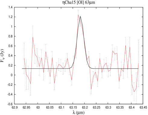
Figure 1: Herschel/Pacs line observations, with overplotted Gaussian to measure the integrated line flux of [OI] 63.18 $\mu$m. All other line observations are non-detections as listed in Table 1. Errorbars indicate the 1 $\sigma$ noise level. The [OI] 63.18 $\mu$m line profile is dominated by the spectral resolution of the PACS spectrometer $R\!\approx\!3000$.

3 Observations and Data Reduction

3.1 Herschel/PACS

Herschel/Pacs observations were obtained for ET Cha during the Science Demonstration Phase. The photometric observations were obtained in the scan map mode in the blue (70 $\mu$m) and the red (160 $\mu$m) filters. Two different scan map angles were used, 45$\degr$ (obsid 1342187338, 133s) and 63$\degr$ (obsid 1342189366, 220s). Both scans were obtained at a medium scan speed of $20\arcsec$/s, with a cross scan step of $5\arcsec$ and scan leg length of 3’. The number of scan legs was 8 for the 63$\degr$ scan, and 4 for the 45$\degr$ scan. For spectroscopic observations, a 1669s PacsLineSpec (obsid 1342186314) and a 5150s PacsRangeSpec (obsid 1342187019) were obtained. The PacsLineSpec provides two simultaneous spectra at wavelengths $62.93\!-\!64.43\,\mu$m, and $180.76\!-\!190.29\,\mu$m. PacsRangeSpec covers six spectral ranges of $71.81\!-\!73.28\,\mu$m, $78.37\!-\!79.76\,\mu$m, $89.28\!-\!90.48\,\mu$m, $143.59\!-\!146.53\,\mu$m, $156.70\!-\!159.47\!\mu$m, and $178.51\!-\!180.96\,\mu$m. Observations were taken in the chop-nod mode, with a small $2\arcsec$ dither. The target was centred at the central spaxel of the $9.4\arcsec\!\times\!9.4\arcsec$ grid of the Pacs Integral Field Unit. The data was reduced using the Herschel Interactive Processing Environment (Hipe; Ott 2010) developer build version 3.0.1212, and the data reduction scripts provided at the Herschel data reduction workshop held in January 2010.

For the photometric data, a mosaic was created from the two scan maps. Aperture photometry was performed using an aperture radius of 16″in the blue, and 19.2″in the red. An aperture correction of 0.922 (blue), and 0.885 (red) was applied to the photometry. The aperture corrections were obtained from the Pacs PhotChopNod Release Note (Feb. 22, 2010). The flux calibration uncertainty is estimated to be 5% in the blue and 10% in the red. For the spectroscopic data, we extracted the spectrum from the central spaxel, and then applied an aperture correction in order to minimise the flux loss in the neighbouring spaxels. Spectra from the central spaxel were extracted for both the A and the B nods. We then applied wavelength binning to each nod spectrum, using a bin size that is half the width of the instrumental resolution. The final spectrum is the mean of the wavelength-binned spectra from the two nods. The absolute flux calibration uncertainty is estimated to be 40%. We have detected the [OI] 63.2$\,\mu$m emission line for ET Cha, while all other lines are undetected (see Table 1). We used the IDL routine MPFITPEAK to fit an error-weighted Gaussian to the observed [OI] 63.2$\,\mu$m line, and measured the integrated flux of the Gaussian line fit. The 1-$\sigma$ error to the line flux was calculated by setting the height of the Gaussian equal to the continuum rms value, and the width equal to the instrumental resolution. The continuum emission at the rest wavelength of 63.18$\,\mu$m was estimated by fitting a first-order polynomial to the spectral region.

3.2 CTIO/ANDICAM photometry

Table 2: Photometric data of ET Cha.

$\lambda\rm\,[\mu m]$	mag.	$F_{\nu}\rm\,[Jy]$	instrument	ref.
used data …
$0.091-0.111$	–	9.81e-6	Fuse (scaled)	GH
$0.111-0.145$	–	2.85e-4	Hst/Cos	GH
$0.145-0.205$	–	1.69e-4	Hst/Cos/Stis	GH
0.442 (B)	15.64	$0.00195\pm 0.0001$	Ctio/Andicam	GD
0.55 (V)	14.68	$0.0046\pm 0.00025$	Ctio/Andicam	GD
0.66 (R)	13.44	$0.0111\pm 0.0005$	Ctio/Andicam	GD
0.82 (I)	12.23	$0.033\pm 0.002$	Ctio/Andicam	GD
1.23 (J)	10.44	$0.107\pm 0.005$	Ctio/Andicam	GD
1.63 (H)	9.79	$0.124\pm 0.006$	Ctio/Andicam	GD
2.19 (K)	9.32	$0.125\pm 0.006$	Ctio/Andicam	GD
3.60	8.38	$0.125\pm 0.003$	Spitzer/Irac	M
4.50	7.91	$0.123\pm 0.001$	Spitzer/Irac	M
5.80	7.42	$0.124\pm 0.003$	Spitzer/Irac	M
8.00	6.51	$0.162\pm 0.001$	Spitzer/Irac	M
24.0	3.52	$0.280\pm 0.003$	Spitzer/Mips	S
$7.6-37$		Spitzer/Irs low resolution spectrum		B,S
70.0	–	$0.18\pm 0.02$	Herschel/PacsPhot	BR
160.0	–	$0.069\pm 0.007$	Herschel/PacsPhot	BR
870.0	–	$<0.036$	Apex/Laboca	NP
unused data …
0.45 (B)	15.07	$0.00399$	MSSSO 2.3m	L,BR
0.558 (V)	13.97	$0.00940$	SAAO 1m	La,BR
0.695 (R)	12.98	$0.0199$	SAAO 1m	La,BR
0.90 (I)	11.77	$0.0494$	SAAO 1m	La,BR
1.24 (J)	10.51	$0.102\pm 0.003$	2Mass	T,NP
1.65 (H)	9.83	$0.125\pm 0.004$	2Mass	T,NP
2.17 (K)	9.43	$0.114\pm 0.004$	2Mass	T,NP
3.80 (L’)	8.14	$0.14\pm 0.006$	Vlt/Icsaac	H,IP
25.0	–	$0.298\pm 0.03$	Iras	I
60.0	–	$0.281\pm 0.04$	Iras	I
70.0	–	$0.137\pm 0.008$	Spitzer/Mips	S
160.0	–	$<0.12$	Spitzer/Mips	G

Detections are listed as $F_{\nu}\pm\sigma$ whereas non-detections are listed as $<$ $3\sigma$. Abbreviations for references, data reduction and flux conversion are: GH $\!=\!$ Greg Herczeg, this paper; GD $\!=\!$ G. Duchêne, this paper; BR $\!=\!$ B. Riaz, this paper; NP $\!=\!$ N. Phillips, this paper; IP $\!=\!$ I. Pascucci, this paper; M $\!=\!$ Megeath et al. (2005); S $\!=\!$ Sicilia-Aguilar et al. (2009); B $\!=\!$ Bouwman et al. (2006); L $\!=\!$ Lyo et al. (2004); La $\!=\!$ Lawson et al. (2002); H $\!=\!$ Haisch et al. (2005); T $\!=\!$ Cutri et al. (2MASS Point Source Catalogue 2003); I $\!=\!$ Moshir et al. (IRAS Faint Source Catalogue 1990); G $\!=\!$ Gautier et al. (2008).

We obtained new simultaneous optical/NIR photometry using the dual-channel ANDICAM instrument on the CTIO 1.3 m telescope on March 6, 2009. Photometric calibration was performed using the PG 1047 Landolt field. Both the optical and near-infrared data were reduced using standard procedures (flat-fielding, cosmetic cleaning, shift-and add). The photometry on ET Cha and the photometric standard was extracted within a 3″aperture and airmass and colour corrections were applying using coefficients from the ANDICAM website in the optical and from Frogel (1998) in the near-infrared. The resulting photometry is listed in Table 2 along with the mid- and far-infrared fluxes adopted in our analysis. The new photometric fluxes are substantially lower than previously published fluxes, see Table 2.

3.3 APEX/LABOCA photometry

An upper limit at $870\,\mu$m has been obtained from new continuum maps of the $\eta$ Chamaeleontis association taken with the LABOCA bolometer array on Apex (Siringo et al., 2009). The data was reduced using the Bolometer array data Analysis (BoA) software, with a pipeline optimised for faint compact sources. Fluxes were extracted within BoA by fitting the amplitude of a beam-sized Gaussian at specified positions within a map with a pixel scale of $4.6\arcsec/{\rm px}$. For each target the flux was extracted at points in a $5\times 5$ rectangular grid centred on the target with a spacing of $37\arcsec$ (twice the beam FWHM). The sample standard deviation of the 24 off-source measurements is the 1-$\sigma$ uncertainty quoted here. Using aperture photometry instead of beam fitting, with a variety of aperture sizes, and aperture corrections computed from the beam, yields very similar results ($9\pm 11\,{\rm mJy}/{\rm beam}$ for apertures with $r={\rm HWHM}$).

3.4 UV observations

ET Cha was observed in the far-ultraviolet with the Cosmic Origins Spectrograph (COS) and in the near-ultraviolet and blue with the Space Telescope Imaging Spectrograph (STIS) on board of the Hubble Space Telescope (HST) as part of the programme “Disks, Accretion and Outflows of T Tau Stars” (P.I. G. Herczeg) on 5 Feb. 2010. The far-ultraviolet observations were obtained with the G130M and G160M gratings with 3891s and 4501s integration times, respectively, to cover the 1140–1790 Å spectral range with a resolution of $\sim$18 000. The data were reduced with the COS calibration pipeline CALCOS and individual segments were combined with the IDL coaddition procedure described by Danforth et al. (2010). The near-ultraviolet and blue observations were obtained with the G230L and G430L gratings with integrations of 45s and 680s, respectively, to cover the 1700-5700 Å spectral range with a resolution of $\sim$2000. The data were reduced with custom-built software in IDL.

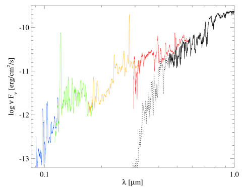
Figure 2: Observed UV spectra and the stellar atmosphere model spectrum for ET Cha (see Sect. 4.1). Blue: Fuse spectrum of TW Hya divided by 20. Green: Hst/Cos spectrum of ET Cha. Orange and red: G230L and G430L Hst/Stis spectra of ET Cha. Black: stellar atmosphere model spectrum with $T_{\rm eff}\!=\!3400\,$K, $\log\,g\!=\!3.89$ and $R_{\star}\!=\!0.84\rm\,R_{\odot}$, at a distance of 97 pc, plotted as dotted line (unused) for $\lambda\!<\!450\,$nm.

A Fuse spectrum of ET Cha covers the spectral region shortward of 1140 Å but has poor signal-to-noise. Instead, the 912–1140 Å flux was estimated from a high-quality Fuse spectrum of TW Hya (Johns-Krull & Herczeg, 2007), scaled to the flux in the 1250–1700 Å bandpass. All different data have been smoothed to a common low resolution, see Fig. 2. Integrated fluxes over three different UV bands as listed in Table 3.

Table 3: Band integrated UV-fluxes for ET Cha.

spectral band [Å]	integrated spectral flux $[\rm\,erg/cm^{2}/s$]
$912-1110$	$8.03\times 10^{-14}$
$1110-1450$	$1.39\times 10^{-12}$
$1450-2050$	$9.73\times 10^{-13}$

3.5 Re-analysis of high-resolution optical spectroscopy

A high-resolution optical spectrum of ET Cha was acquired on June 26, 2002 with the 3.9m Anglo-Australian Telescope Aat and University College London coudé echelle spectrograph (Ucles) as first published by Lawson et al. (2004). A 1.5″slit was used delivering a resolving power of $\sim$30 000 ($10$ km/s at 6300 Å) and covering the wavelength range between 4980 and 9220 Å. The spectrum was calibrated using dome-flats, bias frames and ThAr arc frames, making use of standard library routines such as $\sf ccdproc$ within $\sf IRAF$ (see Lawson et al., 2004, for a detailed description). We have paid particular attention to the removal of telluric contributions to these lines. We removed the OI 6300 Å telluric contribution using the RECX 10 spectrum, a star of similar spectral type but without any evidences of an accretion disk or outflow (Lyo et al., 2003), meaning that the measured OI 6300 Å emission from RECX 10 is thoroughly due to the atmosphere of the Earth.

The average air-masses during observations of ET Cha and RECX 10 are 2.6 and 2.7, respectively. We made a [OI] 6300 Å-map by first removing the [OI] feature from the RECX 10 spectrum, and then subtracting this edited spectrum from the original RECX 10 spectrum. The ET Cha spectrum was divided by the [OI] 6300 Å-map to remove the OI telluric line. We used the photospheric Li I absorption lines at 6707.76 Å and 6707.91 Å to measure a stellar radial velocity of $\sim$22 km/s ($\sim$34.6 km/s after heliocentric correction).

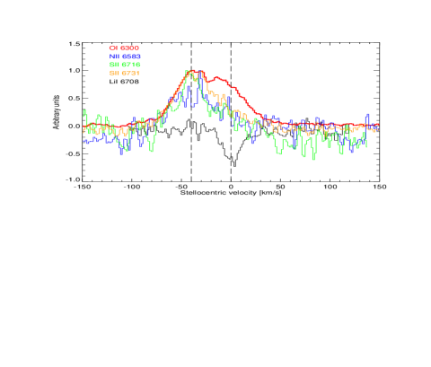
Figure 3: Optical line spectra of ET Cha. All line profiles are continuum subtracted and normalised to line peak emission$\,=\,$1. The forbidden oxygen line [OI] 6300 Å is the strongest emission line by a factor 5 or more, see Table 4, hence the increased noise level in the other lines. The dip in the [OI] 6300 Å line coincides with the position of the telluric component which has been carefully removed, see text. The LiI 6708 Å absorption line has been used to determine the stellar velocity.

Table 4: Measured optical emission line properties.

line	remarks	EW [Å]	$L_{\rm line}\,[10^{-7}L_{\odot}]$	$v_{\rm cen}$	FWHM
$\rm[OI]\,6300\,\AA$	HVC	-6.0	$170-260$	-42	$47\pm\!15$
$\rm[OI]\,6300\,\AA$	LVC	-5.4	$150-230$	0	$38\pm\!15$
$\rm[SII]\,6731\,\AA$	all	-1.8	$50-76$	-35	n.a.
$\rm[SII]\,6716\,\AA$	all	-0.5	$14-21$	-32	n.a.
$\rm[NII]\,6583\,\AA$	all	-0.05	$1.4-2.1$	-40	n.a.

EW$\,=\,$equivalent width, HVC$\,=\,$high-velocity component, LVC$\,=\,$low-velocity component. The luminosity interval corresponds to the uncertainty in the red continuum as derived from photometry $R\!=\!(13.44\!-\!12.98)\,$mag, compare Table 2. Negative values for the centre velocity $v_{\rm cen}$ indicate a blue-shift, n.a. means no values derived. $v_{\rm cen}$ and FWHM are in [km/s].

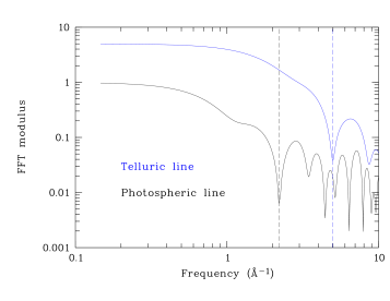
Figure 4: $v_{\rm rot}\sin i$ determination: line profile Fourier transforms. The Fourier transform of a photospheric line at 6709 Å (black line) and a telluric line at 9196 Å (blue line) are shown. The location of the first minimum of the photospheric line profile provides a measurement of $v_{\rm rot}\sin i$. The method requires that the main line broadening mechanism is rotation velocity, that is, the first minimum of the photospheric line must be located at a lower frequency than telluric or arc lines, as shown in the figure. Arbitrary normalisation constants have been applied to the curves to improve readability.

Figure 3 shows the observed profiles of ET Cha in the oxygen line [OI] 6300 Å, with 3 other optical forbidden emission lines overplotted that trace outflows, plus a Li I absorption line to determine the systematic stellar velocity. The [OI] 6300 Å line shows a broad component centred around the stellar systematic velocity (low-velocity component LVC), and a blue component shifted by about 42 km/s (high-velocity component HVC). We have fitted the HVC and LVC by two Gaussian profiles. Measured equivalent widths are listed in Table 4. Equivalent widths for these lines are converted to line luminosities using the procedure outlined in Hartigan et al. (1995), assuming a distance of 97 pc and zero visual extinction. As expected for outflows, the [NII] 6583 Å, [SII] 6716 Å and [SII] 6731 Å emission lines emphasise the HVC, and are all blue-shifted by about the same margin.

Figure 5: Bayesian probability distributions for effective temperature $T_{\rm eff}$, visual extinction $A_{V}$, distance $D$ and stellar radius $R_{\star}$ for ET Cha using our new simultaneous $BVRIJ$ photometry (solid histograms). The vertical dotted lines bracket the range of values explored for each parameter while the vertical dashed line represent the absolute best fit photospheric model.

3.6 Projected stellar rotational velocity

The high resolution spectrum presented in Sect. 3.5 was additionally used to determine the projected rotational velocity of the star $v_{\rm rot}\sin i$. This quantity is typically derived from empirical relations between the full-width at half-maximum of stellar absorption lines and $v_{\rm rot}\sin i$ (see e.g. Martínez-Arnáiz et al., 2010). However, in this paper we use the Fourier transform of the line profile (Gray, D. F., 1992). The full power of this method is revealed in case of very high spectral resolution and signal to noise (Reiners & Schmitt, 2003), but has also been applied successfully to moderate and low quality data (Mora et al., 2001), using the following simplifications.

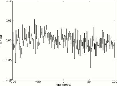
Figure 6: Deep APEX spectrum of ET Cha at 345.796 GHz (866.963 $\mu$m), showing the mean beam temperature $T_{\rm mb}$ versus local standard of rest velocity $v_{\rm lsr}$. The ¹²CO $J\!=\!3\!\to\!2$ line was not detected.

The location of the first minimum of the Fourier transform of any isolated photospheric line profile provides a measurement of $v\sin i$. If many lines are available, the average value and standard deviation can be estimated. The advantage of this method is that the measurements are independent of empirical calibrations and synthetic spectra, provided that enough lines can be identified and the dominant line broadening mechanism is stellar rotation. In terms of Fourier analysis, the latter requirement is equivalent to the following condition: the first minimum of the Fourier transform of photospheric line profiles must be at a smaller frequency than the Fourier transform of lines not affected by rotation velocity (e. g. arc or telluric lines). In addition, the algorithm is robust against the introduction of noise, and capable of working with low signal to noise data.

The method has been applied to the visible Ucles spectrum of ET Cha as described in Sect. 3.5. Few lines could be used for the analysis, due to the low signal to noise ratio ($\sim$10 for unbinned data). A synthetic Kurucz spectrum with physical parameters similar to those listed in Sect. 4.1 was used to identify isolated atomic photospheric lines. After clipping bad lines, only 16 lines remained in the final average used below. Figure 4 shows a sample Fourier transform of both a photospheric and a telluric line to illustrate the method. We obtain

$$v_{\rm rot}\sin i=(15.9\pm 2.0)\ {\rm km/s}\ .$$ (1)

3.7 APEX ¹²CO $J\!=\!3\!\to\!2$

The source was studied in the $J\!=\!3\!\to\!2$ rotational transition of ¹²CO at 345.796 GHz using the Apex telescope and heterodyne receiver system twice, in April and July 2010, for a total on-source time of 100 minutes. A standard on-off switching scheme was used, with reference position $180\arcsec$ off in Azimuth. With an aperture efficiency of $\eta_{\rm mb}\!=\!0.6$, the effective area of the telescope is 67.9 m², and the beam size $\Omega_{A}$ at 345.796 GHz is 13.7$\arcsec$. The CO $J\!=\!3\!\to\!2$ line is commonly detected from disks of radii 100 AU or more; however, in the case of ET Cha, the line was not detected (Fig.6), down to an rms of 17 mK (antenna temperature) for 0.425 km/s wide velocity bins. Assuming the underlying linewidth of the emitting region is 7.5 km/s, as predicted by the best fitting model (Sect. 5) and typical of CO lines from disks, the upper limit to the line flux is $3\sigma=5.5\times 10^{-20}\rm\,W/m^{2}$.

4 Disk modelling

The strong near–mid IR continuum excess of ET Cha (see Fig. 7) as well as the narrow H₂ v$=$1$\to\,$0 S(1) emission line at 2.122 $\mu$m (Ramsay Howat & Greaves, 2007) indicate the presence of a gas-rich protoplanetary disk. The optical high-resolution spectrum with blue-shifted emission lines shows, however, that in addition to the disk, there also exists an outflow that might contribute to the gas emission lines. In the following, we present a combined gas+dust disk model to explore in how far a disk model alone can explain all photometric and spectroscopic observations of ET Cha. The possible contribution of an outflow is discussed in Appendix 6.4.

The disk modelling procedure in this paper consists of three phases. In phase 1, we make a Bayesian analysis, based on the new $BVRIJ$ photometric data, to obtain best fitting values for the stellar parameters. In phase 2, we fix a few more parameters like the inner disk radius based on physical assumptions, e.g., according to stellar luminosity and dust sublimation temperature, and in phase 3, we use the thermo-chemical code ProDiMo (Woitke et al., 2009; Kamp et al., 2009) to calculate the gas- and dust temperature structure in the disk, the chemical and ice composition, and to fit all remaining disk, dust, and gas parameters of the model to the observations as good as possible.

4.1 Stellar parameters

While our new $JHK$ photometry is consistent with the 2 Mass photometry, the $VRI$ photometry is about $0.5\!-\!0.7$ mag fainter than the data published in (Lawson et al., 2002). Indeed, our simultaneous photometry appears to represent the ’faint’ state for ET Cha which, in the accretion hotspot scenario, is purely photospheric.

To estimate the stellar properties, we therefore adopt our new simultaneous photometry. We only fit the $BVRIJ$ fluxes to ensure that our estimates are not biased by the near-IR excess from the disk. We computed a grid of photospheric models, varying $T_{\rm eff}$ (using the $\log g\!=\!4.5$ NextGen models from (Allard et al., 1997), $A_{V}$ (using the $R_{V}\!=\!3.1$-law from Cardelli et al., 1989), $R_{\star}$ and the distance $d$ to ET Cha within generous ranges. The optical extinction is defined by $A_{V}\!=\!2.5\log_{10}({\rm e})\,\tau_{V}$ where $\tau_{V}$ is the optical depth in the visual due to interstellar dust extinction. We note that the last two parameters are degenerate.

The results are shown in Fig. 5. A very good fit is obtained with $T_{\rm eff}\!=\!3300-3400$ K, $d\!=\!97-100$ pc, $R_{\star}\!=\!0.84\!-\!0.89\,R_{\odot}$ (corresponding to $L_{\star}\!=\!0.085\,L_{\odot}$) and $A_{V}\!\leq\!0.2$ mag. This is in excellent agreement with the findings of Luhman & Steeghs (2004), including the effective temperature which they derived exclusively from their spectrum and not from photometry. For the disk modelling, we adopt $T_{\rm eff}\!=\!3400$ K and $R_{\star}\!=\!0.84\,R_{\odot}$, which is both the most probable combination of parameters and the closest to the spectroscopically derived stellar properties.

Finally, we note that conducting the same analysis on the previous photometric dataset (obtained in the “bright” state) yields both a hotter central star ($T_{\rm eff}\!\approx\!\!4000$ K) and a substantial foreground extinction ($A_{V}\!=\!0.75$ mag), both of which are inconsistent with our prior knowledge of the source (see Sect. 2).

In the following, we use the nearest NextGen stellar input spectrum for $T_{\rm eff}\!=\!3400\,$K, $L_{\star}\!=\!0.085\,\rm L_{\odot}$ and solar metallicities (resulting in $\log\,g\!=\!3.89$ and $R_{\star}\!=\!0.84\,\rm R_{\odot}$ for $M_{\star}\!=\!0.2\,\rm M_{\odot}$). According to the stellar evolutionary models of Siess et al. (2000), our choice of $T_{\rm eff}$ and $L_{\star}$ is consistent with a $6\!-\!8$ Myr old star of mass $(0.2\!-\!0.3)\,\rm M_{\odot}$ and solar metallicities.

4.2 Stellar UV-excess

In the UV, stellar activity and mass accretion create an excess emission with respect to classical stellar atmosphere models. Therefore we use our composite observed UV spectrum of ET Cha (Fig. 2) at $\lambda\!<\!450\,$nm as input instead. Although strong Ly$\alpha$ emission from ET Cha was detected with Hst/Cos, no emission was detected near line centre because of neutral hydrogen in our line of sight to the star. Based on an analysis of a similar Ly$\alpha$ emission profile from TW Hya (Herczeg et al., 2004), we roughly estimate that the total flux in this line is twice the detected value. Therefore, we have doubled the detected flux between 1210 Å and 1220 Å for the construction of our UV input spectrum “as seen by the disk”. This yields an integrated flux of $2.22\times 10^{-12}\rm\,erg/cm^{2}/s$ in the 1110–1450 Å band, in contrast to Table 3. We have converted these integrated UV fluxes into additional photometry points, see Table 2, and plotted these points with large errorbars in Fig. 7. These data result in a fractional UV luminosity $f_{\rm UV}\!=\!L_{\rm UV}/L_{\star}\!=\!0.017$ with the UV luminosity $L_{\rm UV}$ being integrated from 912 Å to 2500 Å as introduced by Woitke et al. (2010). The “extra UV” is not important for the spectral energy distribution (SED) modelling, but is essential for the gas modelling, because the UV irradiation is a decisive factor for the gas heating and chemistry in the disk.

4.3 Disk inclination and inner radius

For the disk modelling in Sect. 4.5 we have fixed two parameters to reduce the dimension of parameter space for the fitting problem, namely the disk inclination and inner radius.

First, the disk inclination is assumed to be $i\!=\!40\degr$ as measured from face-on orientation. As long as the disk is not intersecting the line of sight to the star, this parameter does not have a large impact on the model results concerning both SED-analysis and line flux predictions, and we do not have clear observations, e.g., images, that would allow us to determine this quantity unambiguously. Large values for the disk inclination are supported by the H_α line analysis ($60\degr$, Lawson et al., 2004), the low outflow velocities observed (Sect. 3.5), and by the strongly rotation broadened stellar absorption lines (Sect. 3.6), favouring an edge-on rather than a face-on disk orientation.

However, our disk modelling suggests large disk scale heights in the inner disk regions, needed to reproduce the strong near-IR excess (see Fig. 16). For inclinations of 60°and higher, the observer’s line of sight to the central star would therefore intercept the disk. This would cause a dramatic reduction of the observed fluxes at optical and UV wavelengths, as well as a strong reddening of the optical colours. This is inconsistent with our initial assumption that the star is seen directly, used to estimate the stellar properties. In principle, one could increase both the intrinsic stellar luminosity and effective temperature of the star to compensate exactly for this reddening, but to match the observed SED, the required $T_{\rm eff}$ is well beyond values consistent with the M3–M3.5 spectroscopic classification of ET Cha. For inclinations $\ga\!60\degr$ we furthermore observe that the 10 $\mu$m and $20\,\mu$m silicate features are no longer in emission, which clearly contradicts of observed SED of ET Cha.

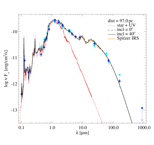
Figure 7: Comparison of model SED to observations. Blue bullets are photometric data points used for the fitting (see Table 2). Light blue symbols refer to other, unused photometry points. Symbols with downward arrows indicate $3\sigma$ upper limits. The black line is the SED from our best-fitting model. The red line shows the assumed stellar input spectrum, completed by piecewise constant fluxes $F_{\nu}$ in three UV bands as obtained by integrating over our UV observations (Table 3).

Second, concerning the disk inner radius, the strong and continuous near-IR fluxes of ET Cha suggest a disk which extends inward close to the star, with no dust holes or gaps. T Tauri disks are generally assumed to be truncated by the stellar magnetosphere near the co-rotation radius, with material accreting along magnetic field lines onto high-latitude regions of the star (Königl, 1991; Shu et al., 1994). From the analysis of optical absorption lines of ET Cha (Sect. 3.6) we have inferred a projected stellar rotation velocity of $v_{\rm rot}\sin i\!=\!(15.9\pm 2.0)\,$km/s. At $i\!=\!40\degr$, this translates into $v_{\rm rot}\!=\!(25\pm 3)\,$km/s (about 12% of the break-up velocity) and, by assuming $M_{\star}\!=\!0.2\rm\,M_{\odot}$ and $R_{\star}\!=\!0.84\,R_{\odot}$ (Sect. 4.1), into a stellar rotation period of $P\!=\!(1.7\pm 0.2)$ days, and a co-rotation radius of $(0.015\pm 0.002)$ AU.

However, the dust temperature at the co-rotation radius ($0.015$ AU) is larger than 1500 K, associated with the sublimation temperature of silicates. Therefore, we have assumed a slightly larger inner disk radius, $R_{\rm in}\!=\!0.022\,$AU, where the dust temperature is about $1500\,$K.

4.4 A single disk model

For a single disk model, we use the radiation thermo-chemical disk code ProDiMo (Woitke et al., 2009; Kamp et al., 2009) to calculate the dust continuum radiative transfer, and the gas thermal balance and chemistry throughout the disk. We use 10 elements, 76 gas phase and solid ice species, and 992 reactions including a detailed treatment of UV-photorates (see Kamp et al., 2009), H₂ formation of grain surfaces, vibrationally excited H${}_{2}^{\star}$ chemistry, and ice formation (adsorption, thermal desorption, photo-desorption, and cosmic-ray desorption) for a limited number of ice species (see Woitke et al., 2009, for details). We also use ProDiMo in this paper to compute all observables including the SED, images, and gas emission line fluxes and profiles. Latest improvements to the ProDiMo model include X-rays chemistry and heating, a parametric prescription for dust settling, UV fluorescent pumping, PAH ionisation and heating/cooling, [OI] 6300 Å pumping by OH-photodissociation, H₂-pumping by its formation on grain surfaces, formal solutions of the line transfer problem, and chemical heating. These improvements are explained in the Appendices A.2 to A.8.

Our modelling of ET Cha is based on a prescribed disk density structure, using power-laws for the surface density distribution and disk flaring, see Appendix A.1. This approach allows for a rapid model computation (avoiding the structure iteration loop, see Fig. 1 in Woitke et al., 2009), and is hence more suitable for a deep search for fitting values in parameter space. In this mode, the disk code uses altogether 25 physical parameters, most of which are considered as fixed for the modelling of ET Cha (for instance the stellar properties, see Table 5).

4.5 Parameter fitting procedure

The determination of the remaining free disk, gas and dust parameters, like the total disk gas mass for instance, is a key objective of the modelling of individual targets. These parameters are “determined” in this paper by considering the values (better the ranges of values) that lead to a satisfying match between predictions and observations in the frame of the model, henceforth called “solutions”. Practically all determinations of properties of astrophysical objects work that way, even if it’s just a simple one-dimensional dependence between property and observable, because the desired quantities are rarely accessible via direct observations. This is the well-known problem of model inversion in astronomy (Lucy, 1994), with all the usual shortcomings and concerns which can be subdivided into four families:

• Concerns about the quality of the model itself (missing physics, poorly determined input quantities like cross-sections and rate coefficients, numerical issues like grid resolution, etc.).
  

• Concerns about the completeness of solutions found in parameter space, for instance, how can we be sure of having found the best solution?
  

• Under-determination, i. e. a weak dependence of observables on model parameters in combination with considerable uncertainties in the observables.
  

• Non-uniqueness of inversion procedure (multiple solutions)

Given the complexity of the disk model at hand, with $8\!-\!14$ free parameters for the modelling of the disk of ET Cha, we have to take into account the possibility that different solutions exist which practically achieve the same degree of agreement between model results and observations. Whereas in a low-dimension parameter space this seems to a be a weird, seldom special case, it occurs frequently in high dimensions, with numerous local minima. The manifold of solutions in a multi-dimensional parameter space can be (and usually is) astonishingly rich and complicated in structure.

Furthermore, it is important to note that, in a high-dimensional parameter space, an exhaustive search is practically impossible. This is even more so for our disk modelling, since one complete model takes about 1 CPU hour on a single 3 GHz processor machine. For 10 parameters, with 20 well-selected values around a main solution each, one would need to run $20^{10}\!\approx\!10^{13}$ models which would take about $1.2\times 10^{9}$ CPU yrs.

Therefore, we are not able to fully devitalise the concerns (1) to (4), but have to face the fact the any parameter determination by model inversion in high-dimensional parameter space is an intrinsically uncertain business. Our strategy in this paper is as follows. We use an evolutionary strategy to find a handful of well-fitting disk models, corresponding to different local minima in parameter space. Among these, we select a “best-fitting” model, the properties of which are described in detail in Appendix C. The best-fitting model is then re-run with different choices of input physics in Appendix D, to explore the principal effects of e. g. X-rays and the treatment of H₂-formation.

We then conclude about the confidence intervals of derived parameter values in Sect. 5 by considering (i) small deviations of single parameters around the best fitting solution, (ii) overall experience from fitting by hand and variance of different solutions found by the evolutionary strategy, and (iii) direct constraints from physical arguments like optical depth and column densities. We admit that this modelling procedure is not entirely satisfactory. A more complete discussion of our modelling strategy will be the topic of a forthcoming paper.

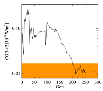
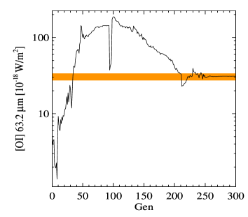
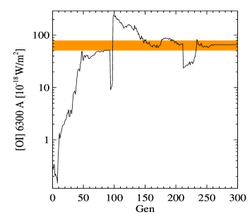
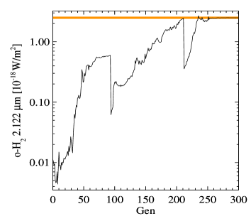
Figure 8: Auto-optimisation of model parameters to fit all continuum and line observations of ET Cha. The first row shows the evolution of some model parameters as function of generation (total gas mass $M_{\rm gas}\,[M_{\odot}]$, total dust mass $M_{\rm dust}\,[M_{\odot}]$, outer disk radius $R_{\rm out}$ [AU]). The two l.h.s. plots in the second row show the resulting $\chi$ for photometry and Spitzer spectrum. The other four plots shows the resulting line fluxes as labelled, where the orange bars indicate the observed line flux ranges with $1\sigma$ errors. At generation 94, the evolutionary strategy got stuck in an unsatisfactory solution (local minimum) with well-fitting SED, but very bad line fits $\chi_{\rm Line}\!\approx\!5$, i. e. a mean deviation between model and observed line fluxes of (e${}^{5}\!\!\approx$150)$\,\sigma$. We have manually changed parameters at generation 95, increasing the disk mass by a factor 10. The evolutionary strategy then found a well-fitting model which can reproduce all available line and continuum observations within about $1\,\sigma$ on average.

4.6 Fit quality and evolutionary strategy

Mathematically, all model inversion techniques can be formulated in terms of a certain strategy to minimise $\chi^{2}$, i. e. to find a minimum of the deviations between model predictions and observations in parameter space. In this paper, we use the following logarithmic measure of these deviations as

$$\displaystyle\chi^{2}=\frac{1}{N}\sum\limits_{i=1}^{N}\Delta_{i}^{2}\quad\mbox{with}$$

$$\Delta_{i}=\left\{\begin{array}[]{ccc}\displaystyle\frac{\log\big{(}F^{i}_{\rm mod}/F^{i}_{\rm obs}\big{)}}{\sigma_{F}^{i}/F^{i}_{\rm obs}}&,&F^{i}_{\rm obs}\geq 3\,\sigma_{F}^{i}\\[14.22636pt] \displaystyle\frac{F^{i}_{\rm mod}}{3\,\sigma_{F}^{i}}&,&F^{i}_{\rm obs}<3\,\sigma_{F}^{i}\ .\end{array}\right.$$ (4)

$F^{i}_{\rm obs}$ and $\sigma_{F}^{i}$ are an observed flux and its uncertainty, and $F^{i}_{\rm mod}$ is the predicted flux by the model. The logarithmic nature of our $\chi^{2}$ is motivated by the need to assign an equally large (bad) number to $\chi$ if a model flux is a factor 10 too large as if it is a factor 10 too small, analog to considering deviations in magnitudes.

Equation (4) is applied separately to all photometric data, all $\lambda$-points in the Spitzer spectrum, and to the line fluxes of CO $J\!=\!3\!\to\!2$, [OI] 63 $\mu$m, [OI] 6300 Å (LVC) and o-H₂ 2.122 $\mu$m, resulting in $\chi^{2}_{\rm Phot}$, $\chi^{2}_{\rm Spit}$, and $\chi^{2}_{\rm Line}$, respectively. The total fit quality of a model is then calculated as

$$\chi^{2}=w^{\rm Phot}\chi^{2}_{\rm Phot}+w^{\rm Spit}\chi^{2}_{\rm Spit}+w^{\rm Line}\chi^{2}_{\rm Line}$$ (5)

with adjustable weights $w^{\rm Phot}$, $w^{\rm Spit}$ and $w^{\rm Line}$, normalised as $w^{\rm Phot}+w^{\rm Spit}+w^{\rm Line}\!=\!1$.

We have applied the $(1,11)$ - evolutionary strategy with adaptive step-size control of Rechenberg (2000) to minimise $\chi$, i. e. to find best-fitting values of our remaining free gas, dust and disk parameters. The strategy uses 1 parent producing 11 offsprings with slightly modified parameters, the best of which will become the parent of the next generation (the parent always dies). The step-size $\delta$ is transmitted to the children and treated as additional parameter to be optimised. After some experiments, we have chosen $w^{\rm Phot}\!=\!0.35$, $w^{\rm Spit}\!=\!0.45$ and $w^{\rm Line}\!=\!0.2$ for optimum performance of the evolutionary strategy.

Figure 8 visualises one exemplary run of the evolutionary strategy, showing the changing model parameters and results over 300 generations. We started from a generic disk setup with $M_{\rm gas}\!=\!10^{-3}M_{\odot}$, gas/dust ratio of 100, and an outer disk radius of $R_{\rm out}\!=\!100\,$AU. This model fails badly to explain the SED and, in particular, the line fluxes. CO $J\!=\!3\!\to\!2$ is about 10 times too strong and both [OI] 6300 Å and o-H₂ 2.122 $\mu$m are more than a factor of 100 too weak. However, after about 300 generations, the model has achieved a good fit of all available continuum and line observations. The final parameter values are far from these initial guesses, yielding a disk that is less than 10 AU in radius and much less massive. All models from about generation 50 onwards fit the dust observations about equally well, the SEDs from these models are almost indistinguishable by eye when plotted as in Fig. 7. A good fit to the line observations was achieved only from generation 200 onward, after the disk radius has shrunk to about $R_{\rm out}\!\la\!10\,$AU while continuing to fit the dust observations about equally well. Thus, the line observations can help to break the degeneracy of SED-fitting.

Table 5: Parameters of the best-fitting disk model.

quantity	symbol	value
stellar mass	$M_{\star}$	$0.2\,M_{\odot}$
effective temperature	$T_{\rm eff}$	$3400\,$K
stellar luminosity	$L_{\star}$	$0.085\,L_{\odot}$
disk gas mass⋆	$M_{\rm gas}$	$6.1\times 10^{-4}\,M_{\odot}$
inner disk radius	$R_{\rm in}$	0.022 AU
outer disk radius⋆	$R_{\rm out}$	8.2 AU
column density power index⋆	$\epsilon$	-0.020
reference scale height⋆	$H_{0}$	0.011 AU
reference radius	$r_{0}$	0.1 AU
flaring power index⋆	$\beta$	1.09
disk dust mass⋆	$M_{\rm dust}$	$2.6\times 10^{-8}\,M_{\odot}$
minimum dust particle radius	${a_{\rm min}}$	$0.05\,\mu$m
maximum dust particle radius	${a_{\rm max}}$	$1\,$mm
dust size dist. power index	$p$	4.1
minimum settling particle size	$a_{\rm s}$	0
dust settling power index	$s$	0
dust material mass density	$\rho_{\rm gr}$	3 g cm-3
dust composition	$\rm Mg_{2}SiO_{4}$	32.9%
(volume fractions)	amorph. carbon	24.4%
	$\rm MgFeSiO_{4}$	23.0%
	$\rm SiO_{2}$	8.8%
	$\rm MgSiO_{3}$	7.6%
	cryst. silicate	3.3%
strength of incident ISM UV	$\chi^{\rm ISM}$	1
cosmic ray H2 ionisation rate	$\zeta_{\rm CR}$	$5\times 10^{-17}$ s-1
PAH abundance rel. to ISM⋆	$f_{\rm PAH}$	0.081
chemical heating efficiency⋆	$\gamma^{\rm chem}$	0.55
$\alpha$ viscosity parameter	$\alpha$	0
disk inclination	$i$	$40\degr$
distance	$d$	97 pc

Parameters marked with ^⋆ have been varied in the evolutionary optimisation run depicted in Fig. 8. The values of the other parameters have been assumed, fitted by hand, or have been obtained from additional evolutionary optimisation runs not discussed here.

Table 6: Computed line fluxes $\rm[10^{-18}\,W/m^{2}]$, at $d\!=\!97$ pc and $i\!=\!40\degr$ from the best-fitting disk model, in comparison to the observations. Non-detections are listed as $<\!3\sigma$ upper limits.

line	$\rm\lambda\,[\mu m]$	observed	model
$\rm[OI]\ ^{3}P_{1}\to\,^{3}P_{2}$	63.18	$30.5\pm 3.2$	34.5
$\rm[OI]\ ^{3}P_{0}\to\,^{3}P_{1}$	145.52	$<6.0$	2.6
$\rm[OI]\ ^{1}D_{2}\to\,^{3}P_{2}$ (HVC)	0.6300	$73\pm 25$	–
$\rm[OI]\ ^{1}D_{2}\to\,^{3}P_{2}$ (LVC)	0.6300	$65\pm 25$	69.6
$\rm[CII]\ ^{2}P_{3/2}\to\,^{2}P_{1/2}$	157.74	$<9.0$	0.11
CO $J\!=\!3\!\to\!2$	866.96	$<0.05$	0.014
CO $J\!=\!29\!\to\!28$	90.16	$<9.6$	4.9
CO $J\!=\!33\!\to\!32$	79.36	$<24$	3.3
CO $J\!=\!36\!\to\!35$	72.84	$<8.0$	2.6
o-H${}_{2}\rm\ v\!=\!1\!\to\!0\ S(1)$	2.122	$2.5\pm 0.1$	2.4
o-H${}_{2}\rm O\ 2_{21}\!\to\!2_{12}$	180.49	$<5.2$	1.1
o-H${}_{2}\rm O\ 2_{12}\!\to\!1_{01}$	179.53	$<5.0$	1.4
o-H${}_{2}\rm O\ 4_{32}\!\to\!3_{12}$	78.74	$<30$	11.1
p-H${}_{2}\rm O\ 3_{22}\!\to\!2_{11}$	89.99	$<9.6$	6.4

5 Results

We identify the result of the evolutionary run depicted in Fig. 8 as our main “best-fitting” model. The resulting parameters are listed in Table 5, the computed line fluxes are summarised in Table 6 and the resulting SED is plotted in Fig. 7. More details about the internal physical and chemical structure of this disk model are shown in Appendix C.

However, the identification of a best-fitting model was not at all straightforward. Altogether 17 runs of the evolutionary strategy have been executed with about 50 to 300 generations each, choosing different parameters to be varied, different initial guesses of the model parameters, or using different setups of the evolutionary strategy. Not all of these runs succeeded to find well-fitting solutions. Some almost equally well-fitting solutions are listed in Table 7. Based on these diverse model inversion results, we have to be very careful with conclusions about the disk properties of ET Cha. The following section summarises our confidence intervals for the various disk shape, dust and gas parameters and discusses which observations are key for their determination.

Table 7: Parameters of different, about equally well-fitting models from different runs of the evolutionary strategy.

parameter	model 1	model 2	model 3	model 4
$M_{\rm gas}\rm\,[10^{-4}\,M_{\odot}]$	0.088	0.65	6.1	25
$M_{\rm dust}\rm\,[10^{-8}\,M_{\odot}]$	3.3	2.6	2.6	3.7
$R_{\rm out}$ [AU]	5.9	7.5	8.2	8.3
$H_{0}$ [AU]	0.0103	0.0096	0.0110	0.0108
$\epsilon$	1.16	0.046	$-0.020$	0.008
$\beta$	1.33	1.15	1.09	1.07
$p$	3.2	3.9	4.1⋆	4.2
$a_{\rm s}\rm\,[\mu m]$	0.05⋆	0.01⋆	0⋆	0⋆
$s$	0.01	0.13	0⋆	0⋆
$f_{\rm PAH}$	0.081	0.098	0.081	0.081
$\gamma^{\rm chem}$	0.14	0.20	0.55	0.09
results
$\chi_{\rm Phot}$	0.48	0.78	0.50	0.45
$\chi_{\rm Spit}$	0.91	0.51	0.51	0.50
$\chi_{\rm Line}$	1.03	1.04	1.25	1.02

Each final model is located in a solid local $\chi$-minimum, the essence after trying a few thousand models. Parameter symbols are explained in Table 5. Other fixed model parameters are as listed in Table 5. Model 3 was selected as best-fitting model. Parameters marked with ^⋆ have been fixed during the evolution.

5.1 Dust mass

ET Cha’s spectral energy distribution (SED) is characterised by a strong near and mid IR excess relative to the star, similar to other much more massive T Tauri disks, see Fig. 7. However, in the far-IR, the fluxes are very faint. 69 mJy at 160,$\mu$m was too weak to be detected by Spitzer, and we have not detected the object at $870\,\mu$m with Apex. Thus, the new Herschel photometry points at $70\,\mu$m and $160\,\mu$m allow for the most complete SED analysis of the source to date.

In all computed disk models for ET Cha, the disk is optically thin at $160\,\mu$m. The observed flux at distance $d$ is hence given by

$$F_{\nu}=\frac{\kappa^{\rm abs}_{\nu}B_{\nu}\big{(}\langle T_{\rm dust}\rangle\big{)}\,M_{\rm dust}}{d^{2}}$$ (6)

where $\langle T_{\rm dust}\rangle$ is the dust mass averaged dust temperature, $\kappa^{\rm abs}_{\nu}$ the dust absorption coefficient in $\rm[cm^{2}/g(dust)]$ and $B_{\nu}$ the Planck function. In the best-fitting model we measure $\langle T_{\rm dust}\rangle\approx 56$ K, and $\kappa^{\rm abs}_{\nu}=34\rm\,cm^{2}/g(dust)$ at 160 $\mu$m, which, according to Eq. (6), results in a 160 $\mu$m flux of 48 mJy which is in good agreement with both, the computed flux from the full disk model (51 mJy) and the observed value of 68 mJy.

Therefore, the observed 160 $\mu$m-flux leaves no doubt that the mass of the dust in the disk of ET Cha must be low, $M_{\rm dust}\!\approx\!2.6\times 10^{-8}\,M_{\odot}$ according to our best fitting model. More massive disks produce too strong 160 $\mu$m continuum fluxes. Although there are certainly some ambiguities in the dust mass determination, e. g. if other dust size parameters are used, leading to a different $\kappa^{\rm abs}_{\nu}$, but among all parameters, $M_{\rm dust}$ certainly belongs to those which are only little influenced by other parameters and can be determined with some confidence. Across all SED-fitting disk models, with varying dust composition and size parameters, the value for $M_{\rm dust}$ ranges in $(2-5)\times 10^{-8}\,M_{\odot}$.

5.2 Dust disk characteristics and particle sizes

According to the low dust mass we derive, the disk of ET Cha has only small optical depths across the disk. Our best-fitting model has vertical dust absorption optical depths $<$1 for $\lambda\!\ga\!4\,\mu$m, except for the optically thick $10\,\mu$m and $20\,\mu$m silicate features. This is valid for all radii since the column density exponent $\epsilon\!\approx\!0$. However, the radial optical depths are much larger. The midplane radial dust extinction optical depth at $1\,\mu$m is about 150. Therefore, the disk of ET Cha is on the borderline between optically thin and thick. It has a complex dust temperature structure due to radial shielding effects (see Fig. 14), but the vertical dust emission could be treated in the optically thin limit at most wavelengths.

Some conclusions about the dust particle sizes can be drawn from the shape of the 10 $\mu$m and 20 $\mu$m silicate features, which are clearly seen in emission for ET Cha (Fig.7). We need a large amplitude of opacity variation across these features (see Fig.13) to model the SED of ET Cha, which favours small, (sub-) micron sized dust particles. Since the peaks are optically thick, warm and small grains must be located in front of cooler dust along the line of sight. We notice that it is easier to fit the observed silicate features with small values of the column density power-law index $\epsilon$, i. e. a roughly flat surface density distribution, and small disk inclinations. For larger $\epsilon$ or larger disk inclinations (closer to edge-on), the silicate features weaken and eventually vanish.

If dust and gas are well-mixed (no dust settling, e. g. models 3 and 4 in Table 7), the models clearly favour very small particles. We can fit the entire SED with a uniform dust population that is either truncated at about 1 $\mu$m, or, alternatively, with a continuous size distribution ranging from 0.05 $\mu$m to 1 mm, but with an unusually large power-law index of $p\!=\!4.1$. The second approach allows for slightly better SED-fits. These findings with ProDiMo have been carefully checked against the Monte Carlo radiative transfer code MCFOST (Pinte et al., 2006, 2009), showing a very good agreement in calculated dust temperatures and continuum fluxes.

However, if dust settling is taken into account (in the approximate way explained in Appendix A.2), Table 7 demonstrates that smaller $p\!=\!3.9$ or even $p\!=\!3.2$ are also possible, in which case the volume-integrated dust size distribution in ET Cha would not be unusual at all, close to the default value of $p\!=\!3.5$. Our honest conclusion about ET Cha is hence that it’s dust must predominantly be made of (sub-) micron particles at the disk surface, where the silicate emission features form. We have therefore decided to refrain from quoting any errorbars to our results concerning the dust size parameters.

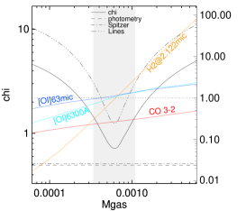
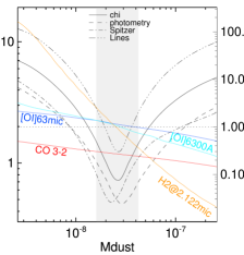
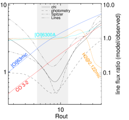
Figure 9: Systematic variation of single parameters around the values of the best-fitting disk model, showing the dependencies on total disk gas mass $M_{\rm gas}\rm\,[M_{\odot}]$ (l.h.s.), on total dust mass $M_{\rm dust}\rm\,[M_{\odot}]$ (middle) and on outer disk radius $R_{\rm out}\,$[AU] (r.h.s.). The full black line shows the total $\chi$, and the dotted, dashed and dashed-dotted lines show its constituents, $\chi_{\rm Phot}$, $\chi_{\rm Spit}$ and $\chi_{\rm Line}$, see Eq. (5). The computed line flux ratios with respect to the observations $F_{\rm line}/F_{\rm obs}$ ($F_{\rm line}/(3\sigma)$ for CO $3\!\to\!2$) are shown by the coloured lines as labelled, with tickmarks on the right axis). The grey shaded box marks the parameter-interval where $\chi$ is not larger than twice its minimum.

5.3 Dust composition

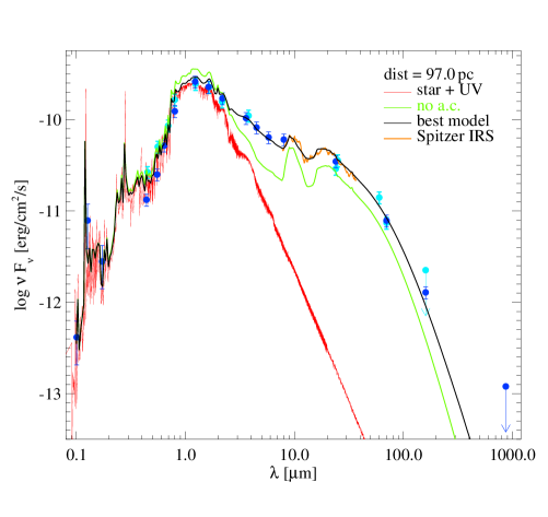
Figure 10: Comparison between predicted SEDs of two models with different dust material composition. The black model shows once more the SED of our best fitting model, with dust composition as listed in Table 5. In the green model, we have omitted the amorphous carbon. All model parameters are identical otherwise.

In our best fitting model, we assume an effective mix of about 33% amorphous fosterite $\rm Mg_{2}SiO_{4}$ (Jäger et al., 2003), 24% amorphous carbon (Zubko et al., 2004), 23% amorphous olivine $\rm MgFeSiO_{4}$ (Dorschner et al., 1995), 9% amorphous silica $\rm SiO_{2}$ (Posch et al., 2003), 8% amorphous enstatite $\rm MgSiO_{3}$ (Dorschner et al., 1995), and 3% crystalline fosterite $\rm Mg_{2}SiO_{4}$ (Servoin & Piriou, 1973). The citations indicate our sources for the complex refractory indexes of the various pure materials. The dust absorption and scattering opacities are calculated by applying effective mixing theory (Bruggeman, 1935) and Mie theory, based on these optical data and volume fractions, and assuming that the chemical dust composition and unsettled dust size distribution is unique throughout the disk. The inclusion of crystalline fosterite is motivated by the fine-structure of the observed second silicate feature at 20 $\mu$m (Bouwman et al., 2006), see (Sicilia-Aguilar et al., 2009), which shows several narrow peaks close to the fosterite peak positions in the data of Servoin & Piriou (1973). The resulting volume fractions are a by-product of our automated fitting procedure from additional runs of the evolutionary strategy not shown in Table 7. We do not claim, however, to have determined the dust composition of ET Cha, as our method is focused on fitting the overall shape of SED rather than individual dust features.

The inclusion of 24% amorphous carbon, however, was an important step to understand the SED of ET Cha. A comparison model without amorphous carbon (green line in Fig. 10) demonstrates its impact on the SED. First, amorphous carbon reduces the dust albedo at UV to near-IR wavelengths (see Fig. 13). Pure laboratory silicates have an albedo of about 80% - 99% around $1\,\mu$m. This leads to a substantial starlight amplification via scattering by the disk at UV to near-IR wavelengths, which is inconsistent with the photometric data. Second, amorphous carbon enhances the absorption and thermal emission in the near-mid IR. As a consequence, the disk is more effectively heated by star light, and produces more thermal emission shortward of the 10 $\mu$m silicate feature, just where ET Cha is very bright, resulting in a much better fit of the SED if we include amorphous carbon. However, any other kind of impurities or inclusions, metallic iron for instance, would cause a similar increase of the dust absorption opacities at optical to near-IR wavelengths, amorphous carbon is just one of the options. The formation of small alien inclusions in the dust material has been demonstrated by Helling & Woitke (2006) and Helling et al. (2006) to be a natural consequence of the refractory dust formation process in somewhat different oxygen-rich environments, namely in brown dwarf atmospheres. Concerning ET Cha we conclude that strong near-IR dust absorption opacities are needed to fit the SED, substantially stronger than those of pure amorphous or crystalline silicates which have a “glassy” character.

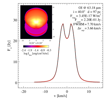
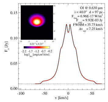
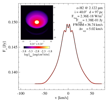
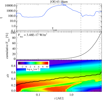
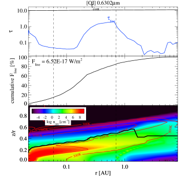
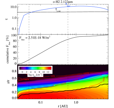
Figure 11: Line profiles, intensity maps, and spatial origin of some emission lines according to the best-fitting disk model. The upper row of figures shows the calculated continuum level, line profile, and continuum-subtracted frequency-integrated line intensity-map for [OI] 63.2$\,\mu$m (left), [OI] 6300 Å (middle) and o-H₂v=1$\to$0 S(1) 2.122 $\mu$m (right), based on formal line transfer solutions at $\rm inclination\!=\!40\degr$. Note the different scaling of velocity axis for the different lines. The lower row of figures visualises the vertical line and continuum optical depths as function of radius, the cumulative line flux, and the species density $\rm[cm^{-3}]$. The vertical dashed lines indicate where the line flux is coming from, bracketing 70% of the cummulative line flux in radius. The thick black lines in the lowest boxes mark those grid cells that contribute most to the vertical line flux; they mark the geometrical depth of the line formation region. For the analysis figures in the lower row, we have directly applied the upwards escape probability formalism (without formal solutions of line transfer). These analyses are hence only approximate in nature and valid for strictly upward line propagation only ($\rm inclination\!=\!0\degr$). The line fluxes calculated in this way deviate from the proper results under $40\degr$ by less than 8%.

5.4 Outer disk radius

Any outer disk radius, at least up to 200 AU, works fine to fit the SED alone. However, the non-detection of CO$\,J\!=\!3\!\to\!2$ and the modest [OI] 63 $\mu$m line flux put severe constraints on $R_{\rm out}$. As Figs. 8 and 9 demonstrate, the CO line flux depends very strongly and robustly on $R_{\rm out}$. All calculated models with $R_{\rm out}\!>\!25$ AU would violate the $3\sigma$ upper limit of CO$\,J\!=\!3\!\to\!2$. Only models with $R_{\rm out}\!<\!10$ AU are consistent with the $1\sigma$ CO line flux upper limit. The CO lines are extremely optically thick, $\tau_{\rm line}\!\approx\!10^{5}$ (see Sect. 5.5). Therefore, even if the CO abundance was reduced by a factor of $10^{3}$ throughout the disk, for example by very efficient CO ice formation, the conclusion that the disk of ET Cha must be small would still be valid. The relatively robust determination of $R_{\rm out}\!\approx\!(6-9)$ AU is demonstrated by Fig. 9 and Table 7. Smaller values of $R_{\rm out}$ are actually inconsistent with the measured [OI] 63 $\mu$m line flux (unless interpreted as originating form an outflow, see Sect. 6.4), because the outer disk is responsible for the [OI] 63 $\mu$m line emission (see Sect. 5.5).

5.5 Spatial origin and characteristics of gas emission lines

Before we continue to conclude about the determination of the disk gas mass of ET Cha, we first have to clarify where the observed spectral lines come from and what they tell us. Figure 11 shows the calculated line fluxes and profiles of the three detected lines [OI] 63 $\mu$m, [OI] 6300 Å (LVC) and o-H₂ 2.122 $\mu$m. We also plot here the vertical line and continuum optical depths and the cumulative line flux as function of radius, to facilitate the discussion of the lines’ spatial origin. These plots are based on the best-fitting disk model, but the drawn conclusions about the spatial origin of the spectral lines are quite general and valid for all calculated disk models that fit the observations of ET Cha.

The far-IR [OI] 63 $\mu$m line probes the outer disk layers, about $2\!-\!7$ AU in this tiny model, and is optically thick with vertical optical depths $\tau_{\rm line}\!\approx\!100\!-\!1000$ in this radial region. The continuum is optically thin. Since the line is collisionally excited, with an excitation energy of about 228 K, the line flux probes first and foremost the existence of warm gas ($T_{\rm gas}\!\ga\!50\,$K) in the disk surface, here at relative heights $z/r\!=\!0.4\!-\!0.5$. In this region, PAH heating is usually the most important heating process. Therefore, this line shows a strong correlation with the assumed PAH abundance, $f_{\rm PAH}$, UV irradiation, and disk flaring.

The optical [OI] 6300 Å line originates from hot gas in the inner disk, about $0.06\!-\!0.7$ AU in this model. As a forbidden line, with very small Einstein coefficient $A_{41}\!\approx\!6.5\times 10^{-3}\rm\,s^{-1}$, it is mostly optically thin $\tau_{\rm line}\!\approx\!0.1\!-\!1$. With an excitation energy of $\sim$15900 K, it probes the existence of hot and dense gas $T_{\rm gas}\!\ga\!3000\,$K in front of an optically thick continuum. To our surprise, this line is not significantly excited by OH photo-dissociation in the model. Neglecting this pumping effect (see Appendix A.5) weakens the [OI] 6300 Å line flux by only 14%. Thus, the [OI] 6300 Å line comes from the bottom of the hot atomic layer, from about $z/r\!=\!0.3\!-\!0.4$ in this model. As soon as molecules form, for example OH and CO, the temperature drops significantly by molecular line cooling, and the [OI] 6300 Å line cannot be excited any longer. Since the line is optically thin, its flux reacts quite sensitively on disk mass. We note that the predicted line $\rm FWHM\!=\!35.7\,km/s$ is in excellent agreement with the observations, $\rm FWHM\!=\!(38\pm 15)\,km/s$, meaning that the spatial origin of the [OI] 6300 Å line is about correct in the model.

The near-IR o-H₂ v=1$\to$0 S(1) 2.122 $\mu$m line also probes the inner disk regions, $0.05\!-\!0.6$ AU in this model. The line is quite optically thick, $\tau_{\rm line}\!\approx\!5\!-\!10$ in this region, where the dust is also optically thick. Since its Einstein coefficient is extremely small, $A_{61}\!\approx\!7\times 10^{-7}\rm\,s^{-1}$, the line needs large H₂ column densities of order $10^{23}\rm\,cm^{-2}$ to become visible over the continuum level. Such column densities are only reached in quite deep layers, $z/r\!\approx\!0.15$, so this line forms in much deeper layers than the [OI] 6300 Å line. The temperature contrast between gas and dust is already quite small in these layers (Fig. 14), which limits the o-H₂ 2.122 $\mu$m line flux. The excitation energy of the line is about 7000 K, i. e. $T_{\rm gas}\!\ga\!1000\,$K is required to collisionally excite it. In the best-fitting model such conditions, $T_{\rm gas}\!\ga\!1000\,{\rm K}\!\gg\!T_{\rm dust}$, are provided by the effect of exothermic chemical reactions (see Appendix A.8) which is active in the warm and dense gas close to the inner rim, deep but not too deep, just where this line forms. Therefore, we see a clear correlation between the o-H₂ 2.122 $\mu$m line flux and the assumed heating efficiency of exothermic reactions $\gamma^{\rm chem}$. The line is also substantially pumped by H₂-formation on grains (see Appendix A.6). When neglecting this effect, the line attains a flux of only 35% of the value from the full model. We conclude that the H₂ line is sensitive to a temperature contrast between gas and dust, and H₂-formation, in quite deep disk layers close to the inner rim. However, the predicted line is too broad ($\rm FWHM\!=\!37\,$km/s) as compared to the observations ($\rm FWHM\!=\!18\pm 1.2$ km/s). We were unable to find any disk model, among the $\sim\!20000$ models computed, that shows such a narrow o-H₂ 2.122 $\mu$m line. Thus, the line forms too close to the star in the model, and we must be very careful when drawing our conclusions about the nature of ET Cha from the observed o-H₂ 2.122 $\mu$m line.

The sub-mm CO$\,J\!=\!3\!\to\!2$ line (not depicted in Fig. 11) probes the size of the disk and the gas temperature in the outermost disk layers. It is massively optically thick, $\tau_{\rm line}\!\ga\!10^{5}$ in the line forming region 2 - 7 AU, where the dust is optically thin. Its flux is roughly proportional to the projected disk area times the gas temperature at relative heights $z/r\!\approx\!0.4\!-\!0.5$ in these outermost parts of the disk.

5.6 Disk gas mass and disk shape

The determination of the total disk gas mass of ET Cha in this paper is based on three detected gas emission lines, namely [OI] 63 $\mu$m, [OI] 6300 Å (LVC), and o-H₂ v=1$\to$0 S(1) 2.122 $\mu$m, which probe complementary radial and vertical disk regions. However, the first line, [OI] 63 $\mu$m, is massively optically thick, and the latter two lines mainly probe the hot gas in the inner disk regions. CO$\,J\!=\!3\!\to\!2$ was not detected. These circumstances immediately suggest that a robust gas mass determination of ET Cha is difficult.

Table 7 shows that various solutions in form of well-fitting disk models can be found where the total gas mass differs by up to two orders of magnitudes (factor 300). A careless reading of Table 7 would suggest that the particular values for $M_{\rm gas}$, $\epsilon$ and $\beta$ do not matter much, but this is not true. Careful inspection of the solutions in Table 7 by systematic variation of selected parameters (see e. g. Fig. 9 for the best-fitting model) shows that these solutions all represent well-defined local minima, where small changes of any parameter leads to a considerable deterioration of the combined line + continuum fit quality $\chi$. If one would measure the uncertainty of gas mass determination from these dependencies alone (for instance the deviation $\Delta M_{\rm gas}$ where $\chi$ doubles) one would arrive at relatively small errors, about 40%. But such an error estimate would be misleading as it would not take into account the complicated manifold of local minima in parameter space.

All solutions in Table 7 fit our entire set of line and continuum observations about equally well. The different values for the gas mass, however, come in certain combinations with other disk shape parameters, like the column density power-law exponent $\epsilon$ and the flaring power $\beta$. Certain fine-tuned combinations of $M_{\rm gas}$, $\epsilon$ and $\beta$ do apparently all provide the proper density and temperature conditions in the disk that result in almost exactly the same observables, for example small $M_{\rm gas}$ in combination with large $\epsilon$ and large $\beta$, or vice versa.

These relations can be understood by minimum column densities of warm H₂ and atomic oxygen in the inner disk parts that are inevitably required to make the [OI] 6300 Å (LVC) and o-H₂ 2.122 $\mu$m lines visible over the strong continuum at optical and near IR wavelengths. For example, in the least massive model 1 in Table 7, there is so little gas in the disk that a relatively large value of $\epsilon\!=\!1.16$ is required to concentrate the mass in the inner disk parts and so to provide the necessary column densities there. All line fluxes are in good agreement with the observations then, but the model has problems to find a good fit of the 10 $\mu$m and 20 $\mu$m silicate features. Also the flaring index of $\beta\!=\!1.33$ is quite extreme, leading to a relative disk height of about $z/r\!=\!1.2$ in the outer disk parts – such a “disk” would be taller than wide. From these arguments, we will discard model 1 from our selection of valid solutions in the following, and claim a minimum gas mass of about $5\times 10^{-5}\rm\,M_{\odot}$ to achieve the necessary minimum gas column densities in the inner disk regions and to fit the silicate dust emission features simultaneously.

Concerning the other direction, we find it hard to provide any solid argument why the disk gas mass must not exceed a certain maximum value. In combination with our quite robust dust mass determination of $M_{\rm dust}\!\approx\!3\times 10^{-8}\,M_{\odot}$, however, even our minimum gas mass of $5\times 10^{-5}\rm\,M_{\odot}$ already implies a very high gas/dust ratio of 2000. An even higher gas mass would translate into an accordingly higher gas/dust ratio. The largest value we found with our evolutionary strategy is $2.5\times 10^{-3}\rm\,M_{\odot}$.

Summarising our modelling efforts, after having tried about 20000 disk models and various choices of input physics, we conclude that the disk gas mass of ET Cha is only little constrained, our confidence interval is about $M_{\rm gas}\!\approx\!(5\times 10^{-5}-3\times 10^{-3})\,M_{\odot}$. The surface density exponent $\epsilon$ and the flaring parameter $\beta$ are likewise poorly constrained, although the models favour small $\epsilon\!\approx\!0$ to fit the silicate dust emission features.

In view of the outflow discussion (Sect. 6.4), we note that the unclear physical origin of [OI] 63 $\mu$m obviously increases our uncertainty in gas mass determination. We have set up a similar evolutionary optimisation run as depicted in Fig. 8, but now treating the [OI] 63 $\mu$m line flux, as emitted by the disk, as an upper limit with $<\!2\times 10^{-18}\rm\,W/m^{2}$. This run resulted in a disk of similar mass as compared to the best-fitting model, $M_{\rm gas}\!=\!5.5\times 10^{-4}\,M_{\odot}$, but of even smaller size $R_{\rm out}\!=\!2.1\,$AU, with an [OI] 63 $\mu$m line flux of $\sim\!4\times 10^{-18}\rm\,W/m^{2}$. We conclude that the [OI] 63 $\mu$m emission line flux is not crucial for the disk gas mass determination of ET Cha, because this disk is tiny and the hot gas is responsible for our detected [OI] 6300 Å (LVC) and o-H₂ 2.122 $\mu$m lines is located in the inner regions. For other, more extended protoplanetary disks, the [OI] 63 $\mu$m line will be less optically thick and hence more useful for the purpose of gas mass determination (Kamp et al., 2010; Pinte et al., 2010; Woitke et al., 2010).

6 Discussion

6.1 Scale heights and unidentified heating

From the SED fitting, we get surprisingly robust results concerning the assumed vertical disk scale height, $H_{0}\!=\!(0.008-0.011)\,$AU at reference radius $r_{0}\!=\!0.1\,$AU, throughout all SED-fitting models. In the model, the reference scale height in combination with the flaring power $\beta$ determines how much star light is captured by the disk. This light (unless scattered away) is absorbed by the dust in the disk surface and then thermally re-emitted, heating also the inner disk parts. Thus, $H_{0}$ regulates the dust temperature in the disk. Since ET Cha is very bright in the $(3\!-\!8)\,\mu$m region, we require large relative scale heights of the order of 10% close to the star to create enough dust emission from warm and hot grains to fit the near and mid IR.

Appendix D.4 (see lower left plot in Fig. 16) demonstrates, however, that our prescribed scale heights are significantly larger, by a factor of 2-3, than those derived from self-consistent models where vertical hydrostatic equilibrium is assumed. This mismatch can be interpreted in three ways: (1) the close midplane regions of T Tauri disks are not in hydrostatic equilibrium, (2) the midplane temperatures are actually 4-9 times higher than assumed in the model (assuming $H\!\propto\!c_{T}\!\propto\!\sqrt{T}$), or (3) there is an additional dust heating process active in the close disk midplane regions that leads to an additional energy flux through the dust component resulting in more observable near-mid IR photons without changing the temperatures much. Possibility 1 cannot be excluded per se. Possibility 2 seems unrealistic because it would cause the dust to evaporate. We favour possibility 3. Appendix D.5 shows that the inclusion of non-radiative dust heating via inelastic gas-dust collisions (thermal accommodation, driven by gas-dust temperature differences created through exothermic chemical reactions) leads to similar effects than increasing the scale height. Because of the $\rho^{2}$-scaling of chemical reactions, this additional heating affects the dust preferentially in high-density regions, increasing the production of near IR photons needed to fit the SED of ET Cha with smaller scale heights. By means of an extra run of the evolutionary strategy, we found out that we can reduce the scale height by about 35% to fit the SED, if we include this effect.

More unidentified dust heating processes may be active in the close midplanes of T Tauri disks. However, viscous heating (according to the formulation by Frank et al., 1992) is not doing a particularly good job in explaining the scale height inconsistencies of ET Cha, see Appendix D.3. Viscous heating dumps additional energy $\propto\!\rho$, i.e., after volume-integration, preferentially into the outer cold regions, leading to the production of more far IR photons. Moreover, viscous heating simply has little effect on the resulting disk temperatures and observable continuum flux in case of low-mass disks as for ET Cha. In fact, the viscous heating according to the formulation by (Frank et al., 1992) produces artifacts in the uppermost tenuous disk layers, where the viscous heating $\propto\!\rho$ cannot be balanced by any cooling $\propto\!\rho^{2}$.

6.2 Effects of other physical processes

Appendix D discusses a number of further physical processes and their influence on the model results that have not been mentioned so far and have not been included in the models discussed so far. To summarise, we find that

(i) X-rays have very little effect (see Appendix D.2) and the neglecting of X-rays in our main model for ET Cha is fully justified. An X-ray luminosity of $L_{X}\!=\!6\times 10^{28}\,$erg/s, as observed for ET Cha (López-Santiago et al., 2010), turns out to be much less important for the disk heating and ionisation as compared to the strong FUV of ET Cha, $L_{\rm UV}\!=\!6.5\times 10^{31}\,$erg/s as measured between 912 and 2500Å, based on our Hst/Cos and Hst/Stis observations.

(ii) The treatment of H₂-formation on grain surfaces is one of the most important yet quite uncertain processes for astrochemical modelling. Appendix D.6 shows that different approaches to calculate the H₂-formation rate lead to a systematic uncertainty in the model for the computation of the o-H₂ 2.122 $\mu$m about a factor of 5. Other spectral lines are less effected.

6.3 Disk inclination and outflow velocity

The low blue-shifts ($-42\,$km/s) seen in the optical emission lines (Fig. 3) are quite unusual for the jets/outflows of T Tauri stars. Typical outflow velocities are $\ga\!100\,$km/s (Hartigan et al., 1995). A possible explanation could be the projection effect in case of a strongly inclined disk (i.e., close to edge-on). Adopting 100 km/s as a lower limit for the outflow velocity of ET Cha would suggest a disk inclination of $>\!65\degr$.

However, as argued in Sect. 4.3, we find that inclinations in the range $0\degr\!-\!50\degr$ are in agreement with the observations, but larger inclinations would result in a partial obscuration of the star by the disk, with dramatic effects on the SED. The SED analysis therefore leads to the conclusion that the inclination of the system, as measured from face-on, is $50\degr$ or less which, in turn, translates to an outflow velocity of 65 km/s at most. If this interpretation is correct, this would make the outflow from ET Cha one of the slowest known outflows from a T Tauri star.

6.4 Outflow and disk lifetime

Our analysis of the optical [OI] 6300 Å and [SII] 6731 Å emission line profiles and fluxes (see Appendix B) results in an estimate of the outflow mass-loss rate of ET Cha of $\dot{M}_{\rm outflow}\!\approx\!10^{-9}\rm\,M_{\odot}/yr$. Such an outflow can contribute to the [OI] 63 $\mu$m emission, which would render the [OI] 63 $\mu$m line flux, as emitted from the disk, smaller as assumed in Sect. 4.5. In summary, Appendix B shows that both approaches, the simple energetic outflow analysis by Hollenbach (1985), as well as the shock models computed by (Hartigan et al., 2004), suggest that the outflow from ET Cha does contribute a substantial, if not dominant, fraction of the observed [OI] 63.2$\mu$m emission line flux. However, without spatially or velocity resolved observations of the outflow, and its subsequent detailed modelling (rather than using some “template” shock models), it is presently impossible to assess the exact contribution of the outflow to the line emission.

Our estimate of the outflow rate of ET Cha is large compared to the total disk mass we derive, $M_{\rm disk}\!\approx\!6\times 10^{-4}\rm\,M_{\odot}$, as it suggests a disk lifetime of only $M_{\rm gas}/\dot{M}_{\rm outflow}\!\approx\!0.7$ Myr, inconsistent with the age of the Chamaeleontis cluster of $\sim\!8\,$Myr. If we would assume a generic gas/dust ratio of 100 and take our dust mass determination for granted, $M_{\rm dust}\!\approx\!3\times 10^{-8}\rm\,M_{\odot}$, it is even worse. The disk lifetime would be even shorter in this case, only 3000 yrs, way too short to be feasible, unless we are just observing a temporary but short-lived 100$\times$ peak in outflow rate.

We also notice that the mass accretion rate of ET Cha was estimated by Lawson et al. (2004) to be equally large, $\dot{M}_{\rm acc}\!\approx\!10^{-9}\rm\,M_{\odot}/yr$ as the outflow mass loss rate, leading to similar lifetime inconsistencies. Furthermore, a branching ratio of $\dot{M}_{\rm outflow}\,/\,\dot{M}_{\rm acc}\!\sim\!1$ is highly unusual, a few percent seems to be a well-established value for T Tauri stars (see e.g. Hartigan et al., 1995).

Murphy et al. (2011) reported on highly variable $H_{\alpha}$ equivalent widths and, accordingly, mass accretion rate, for the old T Tauri stars in the $\eta$ Cha cluster. A factor of 100 variation in the accretion rate is observed in one newly-identified halo member of $\eta$ Cha. But only a simultaneous reduction of both $\dot{M}_{\rm acc}$ and $\dot{M}_{\rm outflow}$ would help to resolve the aforementioned lifetime inconsistency, which doesn’t seem very likely.

One possible explanation would be a massive but short-lived outflow due to a flare from a former epoch, when the mass accretion rate was at least 10 times higher. An outflow of 100 km/s would need $\sim\!50$ yrs to reach a distance of 1000 AU. This would be in agreement with the somewhat slow outflow velocity we derive, $42\!-\!60$ km/s, because the outflow might have slowed down ever since. However, the optical emission lines do not show any evidence for a red-shifted HVC, as one would expect for a symmetric bi-polar outflow. The only plausible explanation of the missing red-shifted HVCs is that these components from the far side are attenuated by the dust in the disk. According to our disk model, the disk is optically thick at 6300 Å up to the outer radius $\sim\!10$ AU (see Fig. 11). Therefore, the line emitting region of the blue-shifted optical emission lines must be quite small, less than 5 AU if seen under 60$\degr$ disk inclination, which corresponds to an age of only 0.25 yr.

7 Summary and conclusions

This paper has reported on new observations of ET Cha with several instruments: Herschel/Pasc, Ctio/Andicam, Hst/Cos/Stis, and Apex. In combination with published data from Spitzer, Gemini/Phoenix and Aat/Ucles, we have collected an unprecedented observational data set about this object, including photometry, UV spectra, high-resolution optical spectrum, near and mid IR spectra, and far IR and sub-mm line fluxes.

We have calculated united gas and dust models for the disk of ET Cha that can simultaneously fit all line and continuum observations, except for a too broad o-H₂ 2.122 $\mu$m emission line profile. The observations also show some blue-shifted components of optical emission lines that point to an outflow and are not included in the models.

This paper has explored the parameter space of the disk models by using an evolutionary strategy to minimise the discrepancies between model predictions and observations. The paper has also introduced a number of basic improvements to the ProDiMo disk modelling code concerning the treatment of PAH ionisation balance and heating, heating by exothermic chemical reactions, several non-thermal pumping mechanisms for selected gas emission lines, and formal solutions of the line transfer problem at given inclination (Appendix A).

From the disk modelling we find a rich variety of fitting disk models that can explain our observations about equally well. Some of the model parameters (like the dust mass and the outer radius) can be determined with some confidence whereas other parameters (like the disk gas mass) are poorly constrained:

• The new Herschel/Pacs photometric fluxes at 70$\,\mu$m and 160$\,\mu$m constrain the disk dust mass of ET Cha to be about $M_{\rm dust}=(2-5)\times 10^{-8}\,M_{\odot}$, putting the object at the borderline between optically thin and optically thick.
  

• Then strong near IR excess of ET Cha can be fitted with a disk that is truncated at $R_{\rm in}\!\approx\!0.022\,$AU (where $T_{\rm dust}\!\approx\!1500\,$K) which is located slightly outside of the co-rotation radius of 0.015 AU. The latter is calculated according to the assumption that the star rotates with a period $P=1.7\,$days as suggested by our $v_{\rm rot}\sin(i)$ analysis of rotationally broadened stellar absorption lines.
  

• From the Apex CO $J\!=\!3\!\to\!2$ non-detection, we can infer, with confidence, that the disk of ET Cha must be tiny in radius. The models favour an outer disk radius as small as $R_{\rm out}\!\approx\!(6-9)\,$AU. All disk models with $R_{\rm out}\!\ga\!25\,$AU would violate the $3\sigma$ CO $J\!=\!3\!\to\!2$ non-detection limit, independent of chemical details.
  

• The SED-fitting suggests that the dust grains in the surface of the protoplanetary disk of ET Cha (where the near-mid IR continuum forms) must be small in radius (sub-micron sized) and opaque in the optical and near-mid IR, i. e. absorption must dominate over scattering opacities. In the models, these spectral properties are provided by the inclusion of about 25% amorphous carbon, but other options like metallic iron are also possible.
  

• The disk gas mass of ET Cha is poorly constrained by our line observations CO $J\!=\!3\!\to\!2$ (non-detection), [OI] 63 $\mu$m, [OI] 6300 Å (LVC), and o-H₂v=1$\to$0 S(1) 2.122 $\mu$m. We find a variety of about equally well fitting disk models with total gas masses $M_{\rm gas}\!=\!(5\times 10^{-5}-3\times 10^{-3})\,M_{\odot}$. The forbidden lines of [OI] 6300 Å (LVC), and o-H₂ 2.122 $\mu$m are close to optically thin and hence quite useful for gas mass determination, but originate from hot gas in the inner disk regions only. [OI] 63 $\mu$m is massively optically thick and does hence not discriminate much between the various disk models for the case of ET Cha. We would need to observe additional far-IR or sub-mm spectral lines that originate from the outer disk parts to determine the gas mass with more confidence. However, in order to explain the [OI] 6300 Å (LVC) and o-H₂ 2.122 $\mu$m lines with a disk model, we require line optical depths $\tau_{\rm line}\!\ga\!1$ which translates into total vertical column densities in the inner disk regions of about $N_{\rm O}\!\ga\!10^{21}\rm\,cm^{-2}$ and $N_{\rm H2}\!\ga\!10^{24}\rm\,cm^{-2}$ for atomic oxygen and molecular hydrogen, respectively. Such column densities are incompatible with $M_{\rm gas}\!<\!5\times 10^{-5}\,M_{\odot}$.
  

• The wide range of fitting gas masses is related to particular values of the disk shape parameters, namely the column density exponent $\epsilon$ and the disk flaring power $\beta$. Large gas masses need to be combined with small values for $\epsilon$ and $\beta$, and vice versa.
  

• From our SED modelling of ET Cha we derive disk scale heights of the order of 10% relative to radius close to the star, which is about a factor of 2-3 larger than the scale heights inferred form self-consistent models that assume hydrostatic equilibrium. This discrepancy can partly be explained by an additional non-radiative heating of the dust close to the star, for example via exothermic chemical reactions.

These results suggest a surprisingly high value for the overall gas/dust mass ratio of ET Cha of at least 2000, or even 20000. Whether or not the gas responsible for the [OI] 6300 Å and o-H₂ 2.122 $\mu$m emissions is still physically connected to the disk is not entirely clear, but the observations show that this gas is at least not moving much with respect to the disk. Possibly, the overwhelming majority of dust particles responsible for the near to far-IR emission of the star has already been transformed into larger pebbles or solid bodies, which have negligible opacities.

The fluxes in blue-shifted emission line components like [OI] 6300 Å (HVC) suggest an outflow with mass-loss rate $\dot{M}_{\rm outflow}\!\approx\!10^{-9}\rm\,M_{\odot}/yr$, on a similar level as the reported mass accretion rate of ET Cha. The low velocities ($\approx\!-42\,$km/s) suggests a high inclination angle of at least 60$\degr$ (rather more). However, inclinations in excess of 50$\degr$ are inconsistent with our SED-modelling, which favours $i\!\la\!40\degr$, from which we determine an outflow velocity of 65 km/s at most (typical values are in excess of 100 km/s for T Tauri outflows Hartigan et al., 1995). If this interpretation is correct, ET Cha would possess one of the slowest known outflows from a T Tauri star.

An outflow with mass loss rate $\dot{M}_{\rm outflow}\!\approx\!10^{-9}\rm\,M_{\odot}/yr$ is likely to contribute significantly to the [OI] 63$\mu$m line flux as observed with Herschel/Pacs. Given the observational data we have collected in this paper, we cannot discriminate between outflow or disk origin of [OI] 63$\mu$m.

To conclude, ET Cha seems to be an extraordinary and puzzling object concerning the evolution of protoplanetary disks. Despite its age of about $(6-8)$ Myr, there is evidence of active accretion onto the central star, on a similar level as the derived outflow mass-loss rate. According to the low disk masses we derive, the disk lifetime $M_{\rm gas}/\dot{M}_{\rm acc}\approx(0.05\!-\!3)$ Myr is inconsistent with cluster age. If a generic gas/dust ratio of 100 was assumed, the disk lifetime, based on our relatively robust determination of the disk dust mass, would be even shorter, only $\sim\!3000$ yrs. Either the object is actually much younger than the age of the Chamaeleontis cluster or the object is going through a phase of unusually high mass accretion rate and outflow.

Appendix A New features in ProDiMo

A.1 Fixed disk structure

In contrast to earlier publications, we use a parametrised description for the shape and distribution of gas and dust in the disk in this paper

$$\rho(r,z)=\rho_{0}\,\Big{(}\frac{r}{r_{0}}\Big{)}^{-\textstyle\epsilon}\frac{H_{0}}{H(r)}\,\exp\Big{(}-\frac{z^{2}}{2\,H(r)^{\,2}}\Big{)}$$ (7)

between an inner and outer disk radius, $R_{\rm in}$ and $R_{\rm out}$, respectively, with sharp edges. $\rho(r,z)$ is the local gas mass density. $H(r)$ is the vertical scale height of the disk, assuming to vary with radius as

$$H(r)=H_{0}\,\Big{(}\frac{r}{r_{0}}\Big{)}^{\,\beta}\ .$$ (8)

$H_{0}$ is the reference scale height at reference radius $r_{0}$. $\epsilon$ is the column density power-law index and $\beta$ the flaring power. The constant $\rho_{0}$ is adjusted such that the integrated disk mass $2\pi\iint\rho(x,z)\,dz\;r\,dr$ equals $M_{\rm disk}$.

A.2 Dust size distribution and dust settling

The dust grains are assumed to have a power-law size distribution in the unsettled case as

$$f(a)\propto a^{\,-p}$$ (9)

between minimum and maximum grain radius, ${a_{\rm min}}$ and ${a_{\rm max}}$, respectively. The free constant in Eq. (9) is adjusted to result in the prescribed unsettled dust/gas mass ratio $\rho_{\rm d}/\rho$.

A very simple recipe has been implemented to account for the major effects of vertical dust settling. We assume that the dust grains are distributed vertically with a smaller scale height

$$H^{\prime}(a,r)=H(r)\cdot\max\big{\{}1,a/a_{\rm s}\big{\}}^{-s/2}$$ (10)

where $H(r)$ is the gas scale height, and $s$ and $a_{\rm s}$ are two free parameters. Since ProDiMo can self-consistently calculate the vertical stratification of gas from the resulting gas temperatures and mean molecular weights, in which case $H(r)$ does not exist, Eq. (10) can not be used directly in the general case. Instead, we make use of the equation that defines $H(r)$, namely $c_{T}\!=\!H(r)\,\Omega(r)$ and write

$$c_{T}^{\prime}(a)=c_{T}\cdot\max\big{\{}1,a/a_{\rm s}\big{\}}^{-s/2}\ ,$$ (11)

where $c_{T}$ is the local gas isothermal sound speed, $c_{T}^{\prime}(a)$ is the reduced variant for dust size $a$, $\Omega\!=\!v_{\rm Kepler}/r$ is the angular velocity and $v_{\rm Kepler}$ the Keplerian velocity. Equation (11) is then used to calculate the vertical distribution of dust particles of different sizes with respect to the already determined gas stratification by treating them like an independent fluids with smaller $c_{T}$ as compared to the gas

$$\frac{1}{\rho^{\prime}(a)}\frac{dp^{\prime}(a)}{dz}=-g_{z}=\frac{1}{\rho}\frac{dp}{dz}$$ (12)

where $p\!=\!c_{T}^{2}\,\rho$ belongs to the gas, and $p^{\prime}(a)\!=\!c^{{}^{\prime}2}_{T}(a)\,\rho^{\prime}(a)$ belongs to dust particles in $[a,a+da]$. $g_{z}$ is the local z-component of gravity. The solution of the differential Eq. (12) is

$$f^{\prime}(a,z)=\frac{{\rm const}(a)}{c^{{}^{\prime}2}_{T}(a,z)}\exp\left(\frac{c_{T}^{2}(z)}{c^{{}^{\prime}2}_{T}(a,z)}\ln\big{(}c_{T}^{2}(z)f(a,z)\big{)}\right)\ ,$$ (13)

where $f^{\prime}(a,z)\,da=\rho^{\prime}(a)/m_{\rm d}(a)$ is the settled dust size distribution function, and $c_{T}(z)$ and $f(a,z)\!\propto\!\rho(z)$ are considered as known. The constant ${\rm const}(a)$ is then determined to make sure that the vertical column density of dust particles for every size is conserved

$$\int f^{\prime}(a,z)\,dz=\int f(a,z)\,dz\ .$$ (14)

According to these assumptions, all dust quantities that used to be constant, such as the local dust/gas mass ratio $\rho_{d}/\rho$, the dust moments $\langle a\rangle$, $\langle a^{2}\rangle$, $\langle a^{3}\rangle$, and the dust opacities per mass, become spatially dependent quantities. The dust absorption and scattering opacities are calculated by applying effective mixing (Bruggeman, 1935) and Mie theory, based on $f^{\prime}(a,z)$.

A.3 PAH ionisation equilibrium and PAH-heating:

We consider a typical size of PAH molecules with $N_{\rm C}\!=\!54$ carbon atoms and $N_{\rm H}\!=\!18$ hydrogen atoms (circumcoronene), motivated by studies that PAHs with much less carbon atoms would not be stable around young stars on timescales of a few Myr. Much larger PAHs are not consistent with the spatial extent of observed PAH emission in various bands (see e.g. Visser et al., 2007). We include PAH^-, PAH, PAH⁺, PAH²⁺ and PAH³⁺ as additional specimen in the chemical reaction network. Circumcoronene is probably among the smallest PAHs that can survive in a disk around Herbig Ae stars (Visser et al., 2007). The following processes are considered in detail: PAH-photoionisation (Tielens, 2005), electron recombination and some charge exchange reactions (Wolfire et al., 2008; Flower & Pineau des Forêts, 2003). These reactions do not change the basic PAH lattice, but only affect the charging of the PAH molecules. Hence, the total amount of PAHs is conserved and treated like an element with given element abundance

$$\epsilon\,({\rm PAH})=f_{\rm PAH}\;X^{\rm ISM}_{\rm PAH}\;\frac{50}{N_{\rm C}}\ ,$$ (15)

where $X^{\rm ISM}_{\rm PAH}=3\times 10^{-7}$ being the standard ISM particle abundance with respect to hydrogen nuclei (Tielens, 2008), and $f_{\rm PAH}$ is the fraction thereof assumed to be present in the disk.

Concerning the photo-ionisation reactions, we consider the PAH absorption cross sections $\sigma_{\rm PAH}^{k}(\nu)\rm\,[cm^{2}]$ from Li & Draine (2001, see their Eqs. 6–12 and A2–A3) with recent updates for the resonance parameters from Draine & Li (2007). We use their neutral PAH cross section for charge $k\!=\!0$, and the charged cross section otherwise. The photo-ionisation rates $\rm[s^{-1}]$ for PAH molecules with charge $k$ are calculated as

$$R^{k}_{\rm ph}(r,z)=\frac{4\pi}{hc}\int_{912\,\AA}^{\lambda\rm thr}\!\!\sigma_{\rm PAH}^{k}(\nu)\;\nu J_{\nu}(r,z)\,Y^{k}_{\nu}\,s_{\nu}(r,z)\;d\lambda$$ (16)

where $\nu\,$[Hz] is the frequency, $J_{\nu}(r,z)\rm\,[erg/cm^{2}/s/Hz/sr]$ the mean intensity as computed by the dust continuum radiative transfer, and $s_{\nu}(r,z)$ the following self-shielding factor

$$\tau_{\nu}^{\rm PAH}(r,z) \approx \epsilon({\rm PAH})\;\langle\sigma\rangle_{\rm PAH}(\nu)\;{\rm Min}\left\{N^{\rm ver}_{{\rm\langle H\rangle}}(r,z),N^{\rm rad}_{{\rm\langle H\rangle}}(r,z)\right\}$$ (17)

$$s_{\nu}(r,z) = \exp\left({-\tau_{\nu}^{\rm PAH}(r,z)}\right)\ .$$ (18)

$N^{\rm ver}_{{\rm\langle H\rangle}}$ and $N^{\rm rad}_{{\rm\langle H\rangle}}(r,z)$ are the radial inward and vertical upward hydrogen nuclei column densities [cm^-2] in the disk, as measured from point $(r,z)$. For simplicity, we put $\langle\sigma\rangle_{\rm PAH}(\nu)=0.5\left(\sigma_{\rm PAH}^{\,0}(\nu)+\sigma_{\rm PAH}^{+1}(\nu)\right)$. The photo-electron yield is taken from (Jochims et al., 1996)

$$Y^{k}_{\nu}=\left\{\begin{array}[]{cl}1&,\;h\nu>IP^{\,k}+9.2\,{\rm eV}\\ \displaystyle\frac{h\nu-IP^{\,k}}{9.2\rm\,eV}&,\;IP^{\,k}+9.2\,{\rm eV}>h\nu>IP^{\,k}\\[5.69054pt] 0&,\;h\nu<IP^{\,k}\end{array}\right.$$ (19)

According to Weingartner & Draine (2001), the ionisation potentials $IP^{\,k}$ depend on PAH-size and charge $k$. Using their Eqs. (1) and (2) for $N_{\rm C}\!=\!54$, the results are $IP^{\,-1}\!=\!3.10\,$eV, $IP^{\;0}\!=\!6.24\,$eV, $IP^{\,+1}\!=\!9.38\,$eV and $IP^{\,+2}\!=\!12.5\,$eV. The formula is an approximation that reproduces the ionisation potential of benzene as the smallest PAH and graphite as infinitely large PAH. The threshold wavelengths are given by $\lambda_{\rm thr}^{k}=hc/IP^{k}$.

With these photo-ionisation and recombination rates, the local particle densities of PAH^-, PAH, PAH⁺, PAH²⁺ and PAH³⁺ are calculated consistently with the gas-phase and ice chemistry, with a considerable influence on the resultant local electron density. Once these particle densities $n_{\rm PAH}^{k}$ have been determined, the total PAH heating rate $\rm[erg/cm^{3}/s]$ can be calculated as

$$\Gamma_{\rm PAH}=\frac{4\pi}{hc}\sum_{k}n_{\rm PAH}^{k}\int\limits_{912\,\AA}^{\lambda_{\rm thr}^{k}}\sigma_{\rm PAH}^{k}(\nu)\;\nu J_{\nu}\,Y^{k}_{\nu}\,s_{\nu}\,\big{(}h\nu-IP^{\,k}\big{)}\;d\lambda$$ (20)

The PAH recombination cooling rate is calculated as

$$\Lambda_{\rm PAH}=\sum_{k}n_{\rm PAH}^{k}\,n_{e}\,k_{\rm PAH}^{k}(T_{\rm g})\,\big{(}1.5\,kT_{\rm g}\big{)}$$ (21)

where $k_{\rm PAH}^{k}(T_{\rm g})\rm\,[cm^{3}\,s^{-1}]$ is the PAH recombination rate coefficient, $n_{e}$ is the electron density and $T_{\rm g}$ the gas temperature. As a general result, we obtain a top-down layered PAH charge structure, with PAH²⁺ in the uppermost layers with reduced PAH-heating, but PAH^- and intensified PAH-heating close to the midplane. For massive disks (unlike ET Cha), where the electron density virtually vanishes in the deepest layers, the PAH charge becomes neutral again in the midplane.

Table 8: Larger non-LTE model atoms. References are as follows: $\Lambda\!=\,$Schöier et al. (2005), NIST$\,=\,$Ralchenko (2009) K$\,=\,$Krems et al. (2006), S$\,=\,$Störzer & Hollenbach (2000)

species	#levels	#lines	coll. partners	references
O I	91	647	p-H2,o-H2,H,H+,e-	$\Lambda$, NIST, K, S
C I	59	117	p-H2,o-H2,H,H+,He,e-	$\Lambda$, NIST
C II	10	31	p-H2,o-H2,H,e-	$\Lambda$, NIST

A.4 Fluorescent UV-pumping

We have replaced the small model atoms for O, C and C⁺ (as listed in Table 4 of Woitke et al., 2009) by larger ones, see Table 8 (this paper), to account for fluorescent UV and optical pumping of the lower levels responsible for the far IR fine-structure lines. The new model atoms have collisional data only among the lowest states, but much more radiative data. The additional energy levels and transition probabilities are taken from the National Institute of Standards and Technology atomic spectroscopic database (Ralchenko, 2009). We selected all evaluated transitions longward of 912 Å. Rovibronic transitions are permitted and their probabilities are of the order of $(1\!-\!10^{6})\rm\,s^{-1}$, much higher than typical collision rates ($\sim$10^-9 s^-1).

Collisional data connecting the two first electronic-excited states ${}^{1}D_{2}$ at 22830 K and ${}^{1}S_{0}$ at 48370 K of neutral oxygen and the three spin-orbit split ground states ${}^{3}P$ exist with electrons and hydrogen atoms as collision partners (Störzer & Hollenbach, 2000; Krems et al., 2006). For C and C⁺, we use the rates collected in the Leiden Lambda database (Schöier et al., 2005), whose collision rates are mostly limited to the ground state electronic levels.

A.5 [OI] 6300 Å -pumping by OH photo-dissociation

Photo-dissociation of OH by absorption of UV photons into the $1\,^{2}\Sigma^{-}$ state, $\lambda\!\simeq\!(973\!-\!1350)\,\AA$, produces an electronically excited oxygen atom O(${}^{1}D$) as

$$\rm OH+h\nu\longrightarrow O(^{1}{\it D})+H,$$ (22)

while absorption into the $1\,^{1}\Delta$ and $3\,^{2}\Pi$ states, $\lambda\!\simeq\!(1100\!-\!1907)\,\AA$, leads to the ground state ${}^{3}P$. According to van Dishoeck & Dalgarno (1984), about 55% of the OH photodissociations by an interstellar UV field result in an O-atom in the ${}^{1}D_{2}$ state, which happens to be the upper level of the 6300 Å line ${}^{1}D_{2}\to\,^{3}P_{2}$. This chemical pumping was suggested by Acke et al. (2005) to play a major role in the formation of the 6300 Å line around Herbig Ae/Be stars. We take this effect into account by introducing a quasi-collisional pumping rate $\rm[s^{-1}]$

$$C_{l\,u}^{\rm chem}=0.55\times n_{\rm OH}\,R_{\rm ph}^{\rm\,OH}\;\big{/}\;n_{\rm O}$$ (23)

where $R_{\rm ph}^{\rm\,OH}$ is the OH photodissociation rate $\rm[1/s]$. We apply Eq. (23) to $l=\{1,2,3\}$, where $1\!=\!^{3}\!P_{2}$, $2\!=\!^{3}\!P_{1}$, $3\!=\!^{3}\!P_{0}$, and $u\!=\!4\!=\!^{1}D_{2}$. We add these excitation rates to the other collisional excitation rates $C_{l\,u}$ (see Sect. 6.1 in Woitke et al., 2009). In writing Eq. (23), we rely on statistical equilibrium and assume that the majority of chemical reaction channels forming OH start from the 3 lowest ${}^{3}P$ levels with $n_{\rm O}\!\approx\!n_{\rm O}(1)\!+\!n_{\rm O}(2)\!+\!n_{\rm O}(3)$, making sure that $n_{\rm O}\left(\frac{n_{\rm O}(1)}{n_{\rm O}}C_{1\,4}^{\rm chem}\!+\!\frac{n_{\rm O}(2)}{n_{\rm O}}C_{2\,4}^{\rm chem}\!+\!\frac{n_{\rm O}(3)}{n_{\rm O}}C_{3\,4}^{\rm chem}\right)=0.55\,\,n_{\rm OH}\,R_{\rm ph}^{\rm\,OH}$, where $\frac{n_{\rm O}(l)}{n_{\rm O}}$ are the fractional populations.

A.6 H₂-pumping by its formation on dust surfaces

The formation of H₂ on grain surfaces liberates the binding energy, causing the newly formed H₂ molecules to leave the surface in a vibrationally highly excited state. Duley & Williams (1986) estimated that the H₂ molecules will be released in vibrational states as high as $\rm v\!\la\!7$, but in the rotational ground state $J\!=\!0$ for p-H₂ and $J\!=\!1$ for o-H₂.

$$\rm H+H+dust\longrightarrow H_{2}(v\!\leq\!7,J\!=\!0/1)+dust$$ (24)

We treat this formation-pumping by

$$C_{l\,u}^{\rm chem}=\alpha*n_{\rm H}\,R_{\rm dust}^{\rm\,H_{2}}\;\big{/}\;n_{\rm tot}$$ (25)

where $R_{\rm dust}^{\rm\,H_{2}}$ is the H₂ formation rate on dust surfaces $\rm[1/s]$, $u$ is the index of the highest state with $\rm v\!\leq\!7$ and $J\!\leq\!1$ that still has collisional de-excitation rates in the database, and Eq. (25) is applied to all states $l\!<\!u$, i. e. to all states that have lower excitation energy than $u$. $n_{\rm tot}$ is the total ortho or para H₂ particle density, respectively, and $\alpha\!=\!n_{\rm o/p-H_{2}}/n_{\rm H_{2}}$ is the prescribed ortho/para-H₂ fraction.

Our formulation of the H₂-pumping, therefore, leads to a constant de-population of all states $l<u$ with a certain timescale $C_{l\,u}^{\rm chem}\rm\,[s^{-1}]$ (simulating the disappearance of H₂ in all states due to other chemical channels that are feeding the H₂ formation) and an equally large population $\rm[cm^{-3}s^{-1}]$ of the state $u$ due to the formation of H₂ on grains.

The condition of state $u$ being collisionally connected avoids artifacts at very low densities, where collisions are rare and the pumping would lead to an almost complete de-population of all low-lying states. According to our current collection of collisional H₂ de-excitation rates, this condition implies $u\!=\!({\rm v}\!=\!3,J\!=\!0/1)$. We checked that our modelling of the o-H₂v=1$\to$0 S(1) line at 2.122 $\mu$m does not depend much on the choice of this upper level $u$ as long as $\rm v\!>\!1$.

A.7 Line transfer

During solving the chemistry and energy balance of the gas, ProDiMo calculates the various level populations of atoms, ions and molecules by means of an escape probability method (see Sect. 6.1.1 in Woitke et al., 2009). These are stored and used later to perform a formal solution of line transfer for selected spectral lines.

The continuum $+$ line radiative transfer equation is given by

$$\frac{dI_{\nu}}{ds}=\kappa_{\nu}^{\rm ext}\big{(}S_{\nu}-I_{\nu}\big{)}\ ,$$ (26)

where $I_{\nu}$ is the spectral intensity and $s$ the distance on a ray. The source function and extinction coefficient are given by

$$S_{\nu} = \frac{\epsilon_{\nu}^{\rm D}+\phi_{\nu}\epsilon_{\nu}^{\rm L}}{\kappa_{\nu}^{\rm ext}}$$ (27)

$$\kappa_{\nu}^{\rm ext} = \kappa_{\nu}^{\rm D}+\phi_{\nu}\kappa_{\nu}^{\rm L}\ .$$ (28)

Assuming isotropic dust scattering, the continuum and line transfer coefficients are given by

$$\epsilon_{\nu}^{\rm D} = \kappa^{\rm abs}_{\nu}B_{\nu}(T_{\rm dust})+\kappa^{\rm sca}_{\nu}J_{\nu}$$ (29)

$$\kappa_{\nu}^{\rm D} = \kappa^{\rm abs}_{\nu}+\kappa^{\rm sca}_{\nu}$$ (30)

$$\epsilon_{\nu}^{\rm L} = \frac{h\nu}{4\pi}n_{u}A_{ul}$$ (31)

$$\kappa_{\nu}^{\rm L} = \frac{h\nu}{4\pi}\big{(}n_{l}B_{lu}-n_{u}B_{ul}\big{)}\ ,$$ (32)

where $\kappa^{\rm abs}_{\nu}$ and $\kappa^{\rm sca}_{\nu}\rm\,[cm^{-1}]$ are the local dust absorption and scattering coefficients, $B_{\nu}$ is the Planck function, $J_{\nu}$ is the local mean intensity (taken from the results of the continuum radiative transfer), $\nu$ is the line centre frequency, $n_{u}$ and $n_{l}$ are the level populations $\rm[cm^{-3}]$ in the upper and lower state, respectively, and $A_{ul}$ and $B_{ul},B_{lu}$ are the Einstein coefficients.

The profile function $\phi_{\nu}\rm\,[Hz^{-1}]$ is assumed to be given by a Gaussian with thermal $+$ turbulent broadening

$$x = {\rm v^{\prime}}+\@vec{n}\cdot{\@vec{\rm v}}$$ (33)

$$\phi_{\nu} = \frac{c}{\nu\sqrt{\pi}\Delta{\rm v}}\exp\left(-\frac{x^{2}}{\Delta{\rm v}^{2}}\right)\ ,$$ (34)

where ${\rm v^{\prime}}$ is the observers velocity with respect to the star along backward ray direction $\@vec{n}$, $\@vec{\rm v}$ is the 3D-velocity of the emitting gas with respect to the star (assumed to be given by Keplerian orbits), and $x$ the local velocity shift. The velocity width is $\rm\Delta{\rm v}^{2}=v^{2}_{th}+v^{2}_{turb}$ and the thermal velocity ${\rm v}_{\rm th}^{2}\!=\!2kT_{\rm g}/m$ where $m$ is the mass of the line emitting species.

We use the same setup of parallel rays as described in Thi et al. (2010b, see their Sect. 2.3), organised in about 150 log-equidistant concentric rings in the image plane, each subdivided into 72 angular segments. Equation (26) is solved numerically on each of these rays in the observer’s frame on 151 velocity grid points to sample v’, where the transport coefficients are pre-calculated on the grid points and later interpolated along the rays, whereas the profile function is always calculated from scratch. The numerical scheme features a variable step size which is controlled by comparing the results after two consecutive steps with the results obtained after one step of double size.

A.8 Chemical heating

By definition, exothermic chemical reactions convert chemical potential energies into heat, whereas endothermic reactions consume internal kinetic energy and actually cool the gas. We calculate this chemical heating/cooling rate $\rm[erg/cm^{3}\!/s]$ as

$$\Gamma_{\rm chem}=\sum\limits_{r}R(r)\,\gamma^{\rm chem}_{r}\,\Delta H_{r}$$ (35)

where $r$ is an reaction index, $R(r)$ is the reaction rate $\rm[1/cm^{3}/s]$ and $\Delta H_{r}$ $\rm[erg]$ is the reaction enthalpy, which is positive for exothermic reactions and negative for endothermic reactions

$$\Delta H_{r}=\sum\limits_{\rm pr}\Delta H_{f}^{0}({\rm pr})-\sum\limits_{\rm ed}\Delta H_{f}^{0}({\rm ed})\ .$$ (36)

$\Delta H_{f}^{0}$ [erg] is the heat of formation of the chemical species involved in the reactions (pr means products, ed means educts). By simplification, we neglect the temperature-dependence of $\Delta H_{f}$, and take the values for the heat of formation for all species from (Millar et al., 1997), who list $\Delta H_{f}^{0}$ [kJ/mol] at 0 K in their Table 2.

The details of exothermic reactions are quite difficult and often not precisely known. The excess chemical binding energy is seldomly released in form of kinetic energy directly (although there are some exceptions like, for example, dielectronic recombination which is radiationless). But in the vast majority of cases, the reaction will create products in some kind of electronic, vibrational and rotational excited states.

The energy temporarily stored in these excitational states can then be either radiated away (in which case the net heating is small), or subsequent collisional processes can thermalise the excess energy. The ratio between these two competing processes depends on the critical density for collisional de-excitation, which depends largely on type and amount of excitation, for example $\sim\!10^{15}\rm\,cm^{-3}$ for permitted electronic transitions down to $\sim\!10^{3}\rm\,cm^{-3}$ for rotational transitions. Further complications arise in possibly large optical depth where created photons cannot escape directly, scatter around and drive secondary processes, with a higher probability to get (partly) thermalised. To avoid all these complications, we have simply introduced an efficiency $\gamma^{\rm chem}_{r}$ in Eq. (35). We also exclude certain types of reactions from Eq. (35): reactions which are known to produce or absorb photons, cosmic ray and cosmic ray-induced reactions, X-ray primary and secondary reactions, reactions on grain surfaces, and reactions which are energetically treated in larger detail elsewhere. Some of the most important reactions are found to be

$$\rm H^{-}+H\to H_{2}+e^{-} \quad\Delta H_{r}\!=\rm\!+3.72\,eV$$ (37)

$$\rm H_{2}+O\leftrightarrow OH+H \quad\Delta H_{r}\!=\rm\!\pm 0.079\,eV$$ (38)

$$\rm H_{2}+H\to H+H+H \quad\Delta H_{r}\!=\rm\!-4.48\,eV$$ (39)

$$\rm H_{2}+H_{2}\to H_{2}+H+H \quad\Delta H_{r}\!=\rm\!-4.48\,eV\ ,$$ (40)

where we put $\gamma^{\rm chem}_{r}\!=\!1$ for the last two “collider” reactions, assuming that these highly endothermic reactions, which only occur in hot gases, are in fact driven by the kinetic energies of the colliding atoms and molecules.

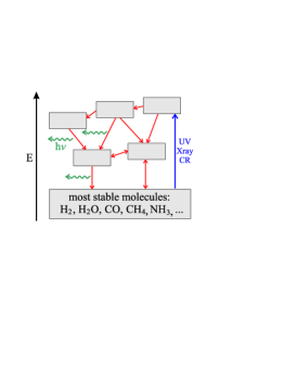
Figure 12: Sketch of energetics in astrochemical reaction cycles.

In kinetic chemical equilibrium, as assumed in this paper, there is no net formation/destruction of any chemical species, but the chemistry is organised in complicated reaction cycles as sketched in Fig. 12. In the absence of cosmic rays, UV photons and X-ray irradiation, only the energetically most favourable chemical configurations, like $\rm H_{2},H_{2}O,CO,CH_{4},NH_{3}$ etc., are abundant. However, due to the impact of these high-energy photons and particles, much less stable molecules, atoms and ions are continuously created which, via some complicated chemical paths, come cascading down in energy again, eventually re-forming the abundant stable molecules. Along these paths, some of the chemical potential energy can be lost in form of secondary photons. The net effect of this cycle is typically a heating, because we have – by definition – excluded the primary UV, X-ray and CR reactions from Eq. (35). The chemical heating is hence yet another way to partly thermalise the energy of incoming high-energy photons and particles through secondary exothermic reactions.

To our surprise, the chemical heating, even with low efficiency $\gamma^{\rm chem}_{r}\!=\!0.1$, results to be an important heating process in protoplanetary disks, in particular at the bottom of the warm molecular layer where many of the near-mid IR spectral lines are formed, and densities are of order $10^{9}-10^{11}\rm\,cm^{-3}$, which, as far we are aware of, has not been noticed so far in other disk modelling papers.

Appendix B The Outflow Model

We have used the HVC [OI] 6300 Å and [SII] 6731 Å line luminosities to estimate the outflow mass loss rate in two independent ways as suggested by Hartigan et al. (1995, see their Eqs. (A8) and (A10)). Assuming the same values for electron density (only necessary for the OI line) and the projected velocity of the jet as used by in Hartigan et al., we obtain an outflow mass loss rate of $\dot{M}_{\rm outflow}\!=\!(0.9\!-\!2)\times 10^{-9}\rm\,M_{\odot}/yr$, similar to the mass accretion rate as estimated by (Lawson et al., 2004).

Hollenbach (1985) showed that it is possible to relate the mass outflow rate to the [OI] 63.2 $\mu$m line luminosity by assuming that each atom in the outflow passes through a single shock wave and that the gas with $T_{\rm g}\!<\!5000$ K cools by radiating only in the [OI] 63.2 $\mu$m line. This procedure is likely to overestimate the resulting line flux since other cooling processes can be active as well, and since the jet material typically passes through several shock waves close to the star. Nevertheless, we use the formula derived by Hollenbach (1985) to obtain a rough estimate of the [OI] 63.2 $\mu$m line luminosity as would be expected for an $\dot{M}_{\rm outflow}\!=\!(0.9\!-\!2)\times 10^{-9}\rm\,M_{\odot}/yr$ outflow. The result is a [OI] 63 $\mu$m line luminosity equal to $(0.6\!-\!1.5)$ times the observed value. This estimate suggests that a substantial part of the [OI] 63.2 $\mu$m line as seen by Herschel might originate in the outflow rather than in the disk. We note, however, that the peak of the HVC is shifted only by about $-42\,$km/s with respect to the stellar velocity, and the formulae used above may not be appropriate to such unusually low outflow/shock velocities.

Another way to estimate the [OI] 63.2 $\mu$m emission line flux from an outflow is to use the shock models of (Hartigan et al., 2004), which predict the line ratio [OI] 6300 Å/[OI] 63.2 $\mu$m for a variety of outflow shock parameters. The authors find 6300/63.2 line ratios of about $(0.8\!-\!2)$. For ET Cha, the measured HVC [OI] 6300 Å line flux is $(37\!-\!87)\times 10^{-18}\rm\,W/m^{2}$, hence the predicted [OI] 63.2 $\mu$m outflow line flux should be $(30\!-\!175)\times 10^{-18}\rm\,W/m^{2}$, which is just consistent with the line flux as observed with Herschel, $(30.5\pm 3.2)\times 10^{-18}\rm\,W/m^{2}$. If we include the LVC and work with the total [OI] 6300 Å emission line flux, the results become inconsistent, i. e. the outflow model alone would already over-predict the measured flux.

Appendix C Details of the best-fitting disk model

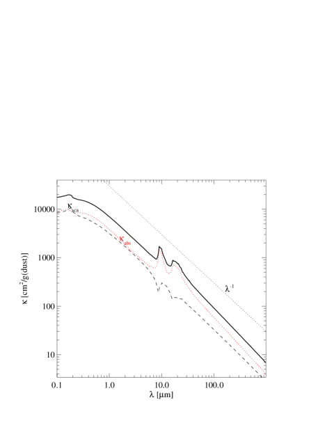
Figure 13: Dust opacities assumed in the best-fitting disk model, calculated with effective mixing and Mie theory according to the parameters listed in Table 5. Note that the absorption coefficient (red dotted) is larger than the scattering (black dashed) also at optical and near IR wavelengths, which is untypical for pure silicates.

Figure 13 shows the dust opacities assumed in the best-fitting model, which results to be absorption-dominated and to scale roughly like $\/\lambda$, except for the 10 $\mu$m and 20 $\mu$m silicate features.

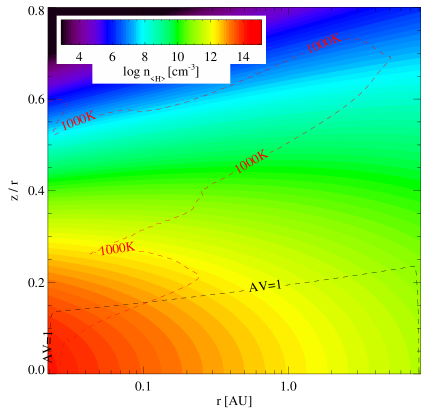
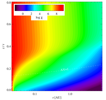
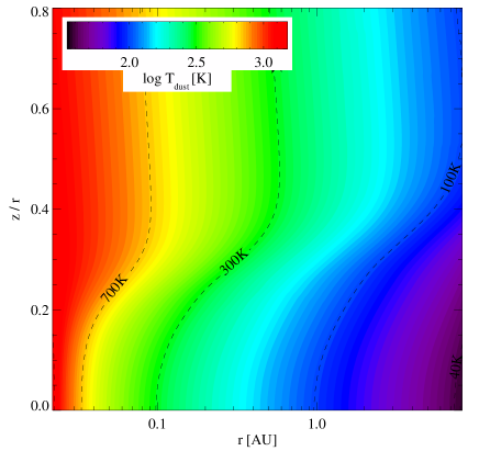
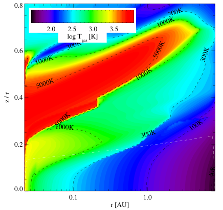
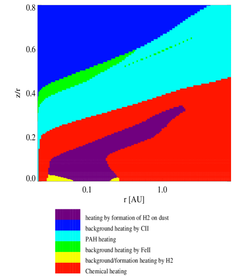
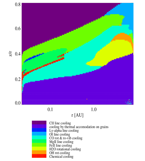
Figure 14: Physical details of the best-fitting disk model. Upper row: total hydrogen nuclei density $n_{{\rm\langle H\rangle}}\rm\,[cm^{-3}]$, with overplotted contours for visual extinction $A_{V}\!=\!1$, and gas temperature $T_{\rm gas}\!=\!1000\,$K, and strength of UV radiation field with respect to interstellar standard $\chi$. Second row: dust and gas temperature structures, $T_{\rm dust}$ and $T_{\rm gas}$ (note the different scaling). Lower row: Most important heating and cooling processes.

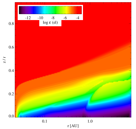
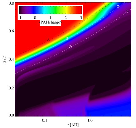
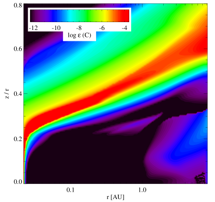
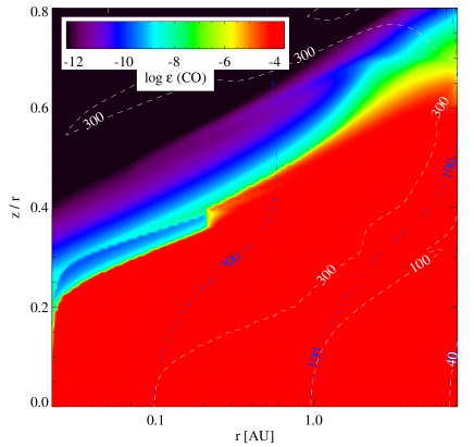
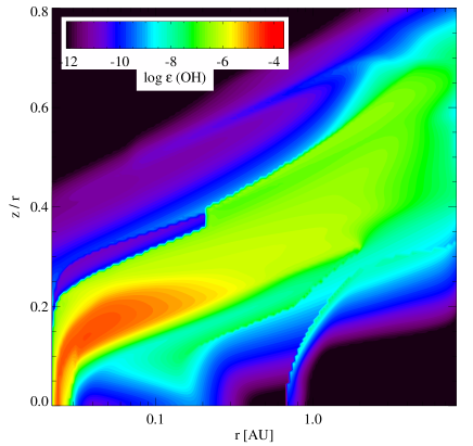
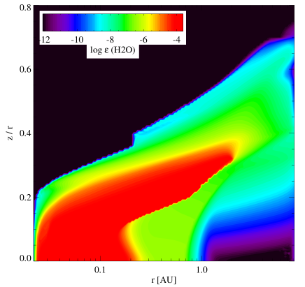
Figure 15: Chemical details of the best-fitting disk model. Upper row: electron concentration $n_{\rm el}/n_{{\rm\langle H\rangle}}$ and mean PAH-charge, with overplotted contours for ionisation parameter $\log(\chi/n_{{\rm\langle H\rangle}})$. Second row: neutral carbon and CO-concentration, the CO-plot includes contours for dust temperature (blue) and gas temperature structure (white). Lower row: OH and H₂O concentration.

Figure 14 visualises the densities, UV radiation field strength, and resulting gas and dust temperatures of the best-fitting model. We obtain the typical $T_{\rm dust}$-pattern for passive disks (see e. g.  Pinte et al., 2009) with a shadow casted by the innermost disk regions and dust temperatures of the order of 1450 K at the inner rim at 0.022 AU, and $\sim\!35\,$K at the outer disk edge located at 8.2 AU. The gas temperature structure $T_{\rm gas}(r,z)$ follows the dust temperature structure in the midplane (where thermal accommodation dominates) but shows substantial deviations at higher altitudes where the disk starts to become optically thin to UV radiation.

In particular, there is a “hot finger” at relative heights $z/r\!\approx\!0.3\!-\!0.6$ in this model, stretching out from the inner rim to about 4 AU in radius. Here, gas temperatures of the order of 5000 K are achieved in this model due to PAH heating versus FeII and MgII line cooling. Just below the hot atomic layer, there is a warm molecular layer with temperatures $300\!-\!1500$K, heated by PAHs and chemical heating, balanced by CO ro-vibrational cooling. The outermost layers beyond 4 AU are featured by an equilibrium between PAH and chemical heating, versus OI, OH, H₂O and CO rotational line cooling.

Figure 15 shows some details about the chemical structure of the disk. There is a quite sudden transition of the charge of the PAHs from 3 to -1 where the ionisation parameter $\chi/n_{{\rm\langle H\rangle}}$ is about 100. The PAHs are mostly negatively charged then, except for the outer midplane where the gas almost completely neutralises. The neutral carbon, CO, OH and H₂O concentrations are typical of a photon dominated region (PDR-structure).

prescribed disk structure	calculated disk structure

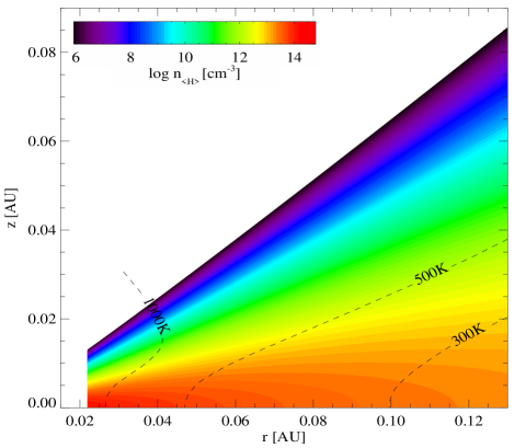
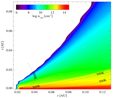
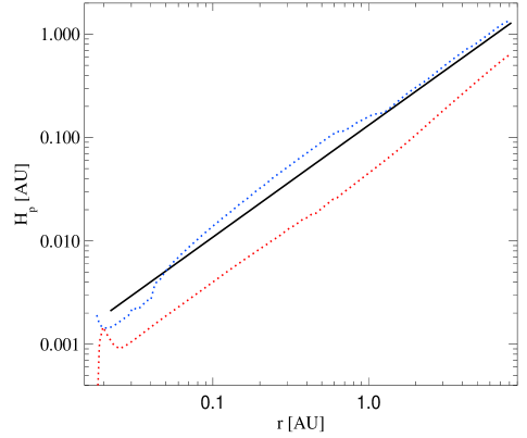
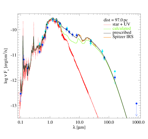
Figure 16: Density structure of inner rim and impact on SED. The upper left plot shows the prescribed density structure of our best-fitting model. Dashed contour lines in the upper panel refer to the calculated dust temperatures. The upper right plot represents a model with identical parameters where, however, the vertical disk structure is calculated consistently with the resultant gas temperatures and mean molecular weights, which results in a flatter midplane close to the star and too little near-mid IR excess (lower right plot). Note the “soft inner edge” (see Woitke et al., 2009). The lower left plot compares the prescribed scale height of the best-fitting model (full line) with the scale heights resulting from the model with calculated vertical disk stratification. The red dotted line shows these results at small relative height $z/r\!=\!0.05$, and the blue dotted line at $z/r\!=\!0.5$.

Appendix D Variation of input physics

D.1 Difference between dust and gas temperature

A control model where the gas temperature is assumed to be equal to the dust temperature resulted in the line fluxes shown in Table 9. We conclude that modelling the gas energy balance, mostly leading to $T_{\rm gas}\!>\!T_{\rm dust}$ in the line forming regions, is absolutely essential to understand the gas emission lines from protoplanetary disks.

Table 9: Computed line fluxes $\rm[10^{-18}\,W/m^{2}]$ from a model where $T_{\rm gas}\!=\!T_{\rm dust}$ is assumed in comparison to the best-fitting disk model.

line	$\rm\lambda\,[\mu m]$	$T_{\rm gas}\!=\!T_{\rm dust}$	best model
$\rm[OI]\ ^{3}P_{1}\to\,^{3}P_{2}$	63.18	5.2	34.5
$\rm[OI]\ ^{1}D_{2}\to\,^{3}P_{2}$ (LVC)	0.6300	2.3	69.6
CO $J\!=\!3\!\to\!2$	866.96	0.0053	0.014
o-H${}_{2}\rm\ v\!=\!1\!\to\!0\ S(1)$	2.122	0.0073	2.4

D.2 Influence of X-rays

We have run a comparison disk model with X-ray heating and chemistry included, as has recently been implemented by Aresu et al. (2010), with X-ray luminosity $L_{X}\!=\!6\times 10^{28}\,$erg/s (Xmm observations by López-Santiago et al., 2010). We assumed an X-ray emission temperature of $T_{X}\!=\!10^{7}\,$K and a minimum energy of X-ray photons of 0.1 keV. This model does not result in any observable changes in the calculated line fluxes. The modification by X-rays are only -0.5%, 1.1%, 1.4% and 0.05% for CO$\,J\!=\!3\!\to\!2$, [OI] 63 $\mu$m, [OI] 6300 Å (LVC) and o-H₂ 2.122 $\mu$m, respectively. Since the X-rays are attenuated by gas in the model, but the UV photons by dust, and our best-fitting model is extremely gas-rich (assumed gas/dust mass ratio $\sim\!23000$, see Table 5), the X-rays do not penetrate deep enough to change the energy balance in the line emitting regions.

D.3 Influence of viscous heating

We have run a comparison disk model with viscous (gas) heating included, via the formula of Frank et al. (1992)

$$\Gamma_{\rm vis}=\frac{9}{4}\,\rho\,\nu_{\rm kin}\,\Omega_{\rm kep}^{2}\ ,$$ (41)

where $\rho$ is the gas mass density, $\nu_{\rm kin}=\alpha\,c_{T}\,H_{p}$ the viscosity, $\alpha$ the viscosity parameter, $c_{T}\!=\!\sqrt{p/\rho}$ the isothermal sound speed, $H_{p}\!=\!c_{T}/\Omega_{\rm kep}$ the pressure scale height, and $\Omega_{\rm kep}\!=\sqrt{GM_{\star}/r^{3}}$ the Keplerian angular velocity. Putting the viscosity parameter to $\alpha\!=\!0.01$, we find no significant changes in the far-IR and (sub-)mm lines, but modest changes in the calculated line fluxes in the optical and near-IR. The enhancement by viscous heating is 1.0%, 2.4%, 25% and 16% for CO$\,J\!=\!3\!\to\!2$, [OI] 63 $\mu$m, [OI] 6300 Å (LVC) and o-H₂ 2.122 $\mu$m, respectively. Since the viscous heating scales as $\Gamma_{\rm vis}\!\propto\!\rho$, but most cooling processes scale as $\Lambda\!\propto\!\rho^{2}$, the effect of the viscous heating is actually strongest in the low density uppermost disk regions, which is counter-intuitive. It renders the gas temperature in these layers unbound (artificially limited by 20000 K), as no implemented cooling process is able to balance the viscous heating according to Eq. (41) in a thin gas. We therefore refrain from discussing the effects of viscous heating any further in this paper.

D.4 Self-consistent disk structure

Figure 16 visualises the density structure as resultant from a self-consistent disk model where the vertical disk stratification is a result of radiative transfer, chemistry, and gas energy balance, assuming vertical hydrostatic equilibrium. We find a good match concerning the flaring angle (the slope in the lower left plot), but a generally flatter disk structure, more condensed toward the midplane. The $z$-dependent scale heights from the self-consistently calculated disk model are calculated as

$$H_{p}^{2}(z)=\frac{z^{2}}{2\,\log\,[p(r,z)/p(r,0)]}\ ,$$ (42)

where $p$ denotes the gas pressure. In the lower left plot of Fig. 16 we have plotted two scale heights from the self-consistent disk model, one measured close to the midplane (at relative height $z/r\!=\!0.05$, red dotted line) and one measured high above the midplane (at $z/r\!=\!0.5$, blue dotted line). The difference between these two scale heights is a natural consequence of our calculated gas temperature structure, with cold conditions in the midplane and a warm/hot disk surface.

We observe a fair match of the scale heights at $z/r\!=\!0.5$ with the prescribed scale-heights from our best-fitting model, but in the midplane the scale heights of the best-fitting model are about a factor of 2-3 too large. Figure 16 also demonstrate that, consequently, we loose our SED-fit when using the self-consistent model. The self-consistent model intercepts less star light, resulting in a significant cooling and flux deficit in the near and mid IR as compared to the observations.

D.5 Influence of non-radiative dust heating

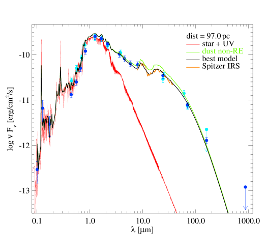
Figure 17: Comparison between predicted SEDs of two models with and without non-radiative dust heating. The black model shows once more the SED of our best fitting model, without non-radiative dust heating. In the green model, non-radiative dust heating through thermal accommodation is included. All model parameters are identical otherwise.

In our best-fitting model, we have ignored non-radiative heating/cooling of the dust grains when determining the dust temperature structure $T_{\rm dust}(r,z)$. However, since the gas is typically warmer than the dust, inelastic gas-grain collisions (thermal accommodation) lead to a collisional, i. e. non-radiative, heating of the dust. If we include this effect (see Eqs. (14) and (108) in Woitke et al., 2009), we do not observe much of an effect on the calculated line fluxes, but the dust temperatures result to be slightly higher, with noticeable effects on the SED, see Fig. 17.

According to this model with the dust in non-radiative equilibrium, the temperature contrast between gas and dust is mainly driven by exothermic chemical reactions which are active even in quite deep and dense layers (see Fig. 14), causing an overall heat transfer from gas to dust in the disk of $\sim\!4.5\times 10^{-3}\rm\,L_{\odot}$, i. e. about 5% of the stellar luminosity. It is this additional energy input that leaves the disk in form of additional mid IR continuum photons, causing the depicted variations in Fig. 17.

The effect of non-radiative dust heating on the SED is similar to increasing the scale heights. We have performed an additional run of the evolutionary strategy with enabled non-radiative dust heating. This run did not entirely converge. The final parameter set had a gas mass of $1.2\times 10^{-3}\rm\,M_{\odot}$, a scale height of only $0.007\,$AU, i. e. a reduction of $\sim\!35\%$ with respect to our best-fitting model. Unfortunately this is a slow and unstable option, because there is an additional outer iteration necessary between gas and dust temperature determination, to achieve consistent results, which requires about 3 times more computational time.

D.6 Influence of treatment of H₂-formation

The formation of H₂ on dust grain surfaces is one of the most important first steps to initiate a rich molecular chemistry. It has profound effects also on other abundances, for instance the C⁺/C/CO transition (because of the mutual H₂/C shielding) and on the formation of OH and H₂O. Yet its rate is still rather uncertain. Our default choice is to calculate this key chemical process according to (Cazaux & Tielens, 2004, called “model B” in Table 10). We have run two comparison models with two other formulations, one with a typically smaller H₂-formation rate according to (Sternberg & Dalgarno, 1995). And one with a typically larger rate according to (Cazaux & Tielens, 2010).

Concerning the formulation of Sternberg & Dalgarno (1995), which is valid for standard ISM size distribution and dust/gas ratio only, we add a scaling factor to account for deviations of the total dust surface per hydrogen nucleus in disks as

$$R_{\rm H2}^{\rm\,form}=3\times 10^{-18}n_{{\rm\langle H\rangle}}\sqrt{T_{\rm gas}}\;\;\frac{\langle a^{2}\rangle\,n_{\rm dust}/n_{{\rm\langle H\rangle}}}{5.899\times 10^{-22}{\,\rm cm^{2}}}\ .$$ (43)

The H₂-formation rate coefficient $R_{\rm H2}^{\rm\,form}\,\rm[1/s]$ needs to be multiplied by the neutral hydrogen atom density $n_{\rm H}$ to get the H₂-formation rate in $\rm[cm^{-3}\,s^{-1}]$. The normalisation factor in Eq. (43) results from $\langle a^{2}\rangle_{\rm ISM}\,[n_{\rm dust}/n_{{\rm\langle H\rangle}}]_{\rm ISM}\!=\!5.899\times 10^{-22}{\rm cm^{2}}$ under interstellar conditions, i. e. for $a_{\rm min}\!=\!0.005\,\mu$m, $a_{\rm min}\!=\!0.25\,\mu$m, $p\!=\!3.5$, $\rho_{\rm gr}\!=\!3\rm\,g/cm^{3}$ and $\rho_{\rm dust}/\rho_{\rm gas}=0.01$.

Table 10 shows a strong dependence of the predicted o-H₂ 2.122 $\mu$m line on the assumed H₂-formation rate on grains. The Sternberg & Dalgarno (1995)-formalism results in a factor of 0.77 smaller and the Cazaux & Tielens (2010)-formalism in a factor of 4.8 larger line flux. This is a daunting example of hidden uncertainties in astrochemical modelling. We note that the Sternberg & Dalgarno (1995)-formalism gives a smaller $\rm FWHM\!\approx\!30\,km/s$ that brings this model closer to the observations. All other calculated gas emission lines (including those of H₂O) are less affected.

Table 10: Calculated o-H₂ and o-H₂O line fluxes $\rm[10^{-18}\,W/m^{2}]$ and FWHM $\rm[km/s]$ of models with different treatment of the H₂-formation on grain surfaces.

	o-H2 2.122 $\mu$m		o-H2O 179.53 $\mu$m		o-H2O 78.74 $\mu$m
	flux	FWHM	flux	FWHM	flux	FWHM
model A	1.81	30	1.41	8.2	11.2	8.5
model B	2.35	37	1.40	8.2	11.1	8.5
model C	11.3	41	1.51	8.3	12.2	8.6
observed	$2.5\!\pm\!0.1$	$18\!\pm\!1.2$	$<5.0$	$-$	$<30$	$-$

model A $=$ Sternberg & Dalgarno (1995), model B (best-fitting model) $=$ Cazaux & Tielens (2004), model C $=$ Cazaux & Tielens (2010). The other calculated gas emission lines are less affected.