Scattering of a proton with the Li₄ cluster: non-adiabatic molecular dynamics description based on time-dependent density-functional theory.

Abstract

We have employed non-adiabatic molecular dynamics based on time-dependent density-functional theory to characterize the scattering behaviour of a proton with the Li₄ cluster. This technique assumes a classical approximation for the nuclei, effectively coupled to the quantum electronic system. This time-dependent theoretical framework accounts, by construction, for possible charge transfer and ionization processes, as well as electronic excitations, which may play a role in the non-adiabatic regime. We have varied the incidence angles in order to analyze the possible reaction patterns. The initial proton kinetic energy of 10 eV is sufficiently high to induce non-adiabatic effects. For all the incidence angles considered the proton is scattered away, except in one interesting case in which one of the Lithium atoms captures it, forming a LiH molecule. This theoretical formalism proves to be a powerful, effective and predictive tool for the analysis of non-adiabatic processes at the nanoscale.

1 Introduction

The study of the interaction of charged particles with matter is a fundamental area in modern physics, since these collisions are relevant for many fields of Science. Two relevant examples are radiation damage in biological tissues, and the stopping power of solids – essential in the design, for example, of fusion devices. In addition to the relatively old areas of ion-atom [1] and ion-surface [2] collisions, the more recent intermediate discipline of ion-cluster collisions [3] has been developed in the last decades.

In general, these processes – not only ion-cluster collisions, but all scattering events of couples of nanoscaled objects, whether they are atoms, clusters or molecules, charged or not – may trigger numerous processes, involving many of the degrees of freedom of the colliding projectiles: transfer of vibrational energy, transfer of electronic charge, ionization, fragmentation (sometimes referred to as collision induced dissociation), recombination, fusion betweeen clusters, electronic excitations, etc.

Perhaps the most important distinction that can be made is between adiabatic and non adiabatic processes. The latter involve electronic excitations, and this fact implies, from a theoretical point of view, the necessity of a much more sophisticated method. If we constrain our consideration to ab initio techniques, adiabatic processes could in principle be studied with standard adiabatic first principles Molecular Dynamics (MD); however, whenever charge transfer, ionization, or simply electronic excitations play a role, some form of non-adiabatic treatment must be used.

One such technique is Ehrenfest MD: it consists of assuming a classical approximation for the nuclei, that are coupled to the quantum electronic system. The latter is still a many-particle system whose out of equilibrium first-principles description is very demanding. It can be studied, however, ab initio and non-adiabatically with the help of time-dependent density-functional theory (TDDFT) [4, 5], that offers a good balance between computational effort and accuracy. This idea has received, among others, the names of Ehrenfest-TDDFT (E-TDDFT), non-adiabatic quantum MD (NA-QMD), or TDDFT-MD.

The first application of the E-TDDFT equations was however in the realm of solid state physics [6], and in fact with the purpose of performing adiabatic MD in a different manner. Their use for non-adiabatic processes was pioneered by Saalmann and Schmidt [7]; a formal derivation of the model by Gross, Dobson and Petersilka can be found in Ref. [8]. It has later been applied to various collision problems: ion-fullerene collisions [9], atom-sodium cluster collisions [10], charge transfer in atom-cluster collisions [11, 12], the stopping power of protons or antiprotons in clusters [13, 14] or insulators [15], the excitation and ionization of molecules such as ethylene due to proton collisions [16], or the interaction of protons or heavier ions with carbon nanostructures or graphitic sheets [17, 18]. It may also be used to study laser-induced molecular or cluster dynamics in the high-field (but still not relativistic) regime; some examples are Refs. [19, 20, 21, 22, 23, 24, 25].

In this work, we have focused on the collision of protons with the lithium tetramer. We investigate the feasibility of using the E-TDDFT approach for identifiying the various possible reaction channels: these collisions are nothing else than chemical reactions with various possibles outcomes, that depend on the initial velocity, impact parameter, relative orientations, and even the initial vibrational state. Depending on the nature of the reactants and on their relative velocity, the reaction may be non-adiabatic, meaning that the electronic excited states play a role. A fully unconstrained first principles study of these chemical reactions in real time is far from possible – the complete study would require running over all possible initial velocities, orientations, etc – but the E-TDDFT model may provide some information for selected initial configurations. Moreover, the current experimental advances in ultra-fast time-resolved observations of chemical reactions in real time demand parallel theoretical tools.

In Section 2 we briefly recall the theoretical framework and the computational methodology; Section 3 describes the results; finally we summarize in Section 4.

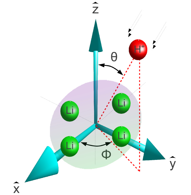
Figure 1: Li₄ tetramer (green atoms) and incident proton (red atom). The proton is always directed towards the center of the tetramer; the incidence angles are $(\phi,\theta)$.

2 Methodology

The Ehrefest MD scheme is defined by the following equations (atomic units are used hereafter):

$$i\frac{\partial}{\partial t}\varphi(x,t) = \hat{H}_{\rm e}(R(t))\varphi(x,t)\,,$$ (1)

$$M_{J}\frac{{\rm d}^{2}}{{\rm d}t^{2}}\vec{R}_{J}(t) = -\!\int\!\!\!{\rm d}x\;\varphi^{*}(x,t)\nabla_{J}\hat{H}_{\rm e}(R(t))\varphi(x,t)$$ (2)

$$-\nabla_{J}\sum_{L\neq J}\frac{Z_{J}Z_{L}}{|\vec{R}_{J}(t)-\vec{R}_{L}(t)|}\,,$$

where $\varphi(x,t)$ is the many-electron wavefunction, that depends on all the electronic degrees of freedom, denoted $x$. It is governed by the electronic Hamiltonian $\hat{H}_{\rm e}(R(t))$, which is determined by all the classical nuclear positions $R(t)\equiv\{\vec{R}_{1}(t),\dots,\vec{R}_{M}(t)\}$. The motion of the nuclei is determined by the set of equations (2) – which are Newton’s equations of motion for each nucleus $J$ (characterized by a mass $M_{J}$ and a charge $Z_{J}$). The electronic Hamiltonian is given by:

$$\hat{H}_{\rm e}(R(t)) = \sum_{j=1}^{N}\frac{-1}{2}\nabla_{j}^{2}+\sum_{j<k}\frac{1}{|\hat{\vec{r}}_{j}-\hat{\vec{r}}_{k}|}$$ (3)

$$-\sum_{Jj}\frac{Z_{J}}{|\vec{R}_{J}(t)-\hat{\vec{r}}_{j}|}\,.$$

The $N$ vector operators $\hat{\vec{r}}_{j}\;(j=1,\dots,N)$ are the electronic position operators. This form of the Hamiltonian allows to write the force that acts on each nucleus solely in terms of the electronic density $n(\vec{r},t)$, i.e., we can rewrite Eqs. 2 as:

$$M_{J}\frac{{\rm d}^{2}}{{\rm d}t^{2}}\vec{R}_{J}(t) = -\!\int\!\!\!{\rm d}^{3}r\;n(\vec{r},t)\nabla_{J}v_{\rm ne}(\vec{r},R(t))\,,$$ (4)

$$-\nabla_{J}\sum_{L\neq J}\frac{Z_{J}Z_{L}}{|\vec{R}_{J}(t)-\vec{R}_{L}(t)|}$$

$$n(\vec{r},t)=\langle\varphi(t)|\sum_{i=1}^{N}\delta(\vec{r}-\hat{\vec{r}}_{j})|\varphi(t)\rangle\,.$$ (5)

The electron-nucleus potential $v_{\rm ne}$ is given by:

$$v_{\rm ne}(\vec{r},R(t))=-\sum_{J}\frac{Z_{J}}{|\vec{R}_{J}(t)-\vec{r}|}\,.$$ (6)

The possibility of computing the ionic forces solely in terms of the electronic density permits to use TDDFT, and propagate the proxy Kohn-Sham (KS) system of non-interacting electrons instead of the real one. Therefore, we no longer propagate Eq. 1, but rather the time-dependent KS equations:

$$i\frac{\partial}{\partial t}\varphi_{i}(\vec{r},t)=\{-\frac{1}{2}\nabla^{2}+v_{\rm KS}[n](\vec{r},t)\}\varphi_{i}(\vec{r},t)\;\;\;(i=1,\dots,N/2)\,$$ (7)

$$n(\vec{r},t)=\sum_{i=1}^{N/2}2|\varphi_{i}(\vec{r},t)|^{2}\,.$$ (8)

Here, we have assumed an even number of electrons $N$, and a spin-restricted configuration in which all the KS spatial orbitals $\varphi_{i}$ are doubly occupied. The non-interacting electrons move in the KS potential $v_{\rm KS}[n](\vec{r},t)$, which is divided into the following terms:

$$v_{\rm KS}[n](\vec{r},t)=v_{\rm ne}(\vec{r},R(t))+\int\!\!{\rm d}^{3}r^{\prime}\frac{n(\vec{r}^{\prime},t)}{|\vec{r}-\vec{r}^{\prime}|}+v_{\rm xc}[n](\vec{r},t)\,.$$ (9)

The last term, $v_{\rm xc}[n](\vec{r},t)$, is the exchange and correlation potential, whose precise form is unknown and must be approximated. In this work we have chosen to use the simplest form, the adiabatic local-density approximation [26].

We have used the octopus code to run these equations. The numerical details can be found in Refs [27, 28]; here we will only summarize the essential aspects: In this TDDFT implementation, the wave functions, densities and potentials are discretized in a real space grid, instead of being expanded in basis sets. One important simplification arises from the use of pseudo-potentials (of the Troullier-Martins [29] type in this work), which substitute the nucleus and the core electrons of the system by a smooth set of local and non-local effective potentials, which are seen by the valence electrons. The Coulomb discontinuity disappears, and the valence orbitals no longer need to be orthonormal to the core ones. These facts allow for the use of a real space grid with a relatively large grid spacing (0.25Å  in this work). The molecule must then be placed in a simulation box, which is a sphere of 20Å  for the simulations that we present here.

The first step in the simulation is the obtention of the ground-state of the Li₄ cluster – both the lowest energy ionic geometry and the corresponding electronic structure. The former is a rhombic planar D_2h geometry (see Fig. 1, the bond length is 2.92Å). The proton is then placed 18Å  away from the centre of the cluster, and is given an initial relative velocity of 0.02 a.u, which corresponds with a kinetic energy of 10 eV. The E-TDDFT equations are then propagated, and we have chosen a total simulation time $T$ of 300 $\hbar$/eV $\approx$ 200 fs. In order to numerically propagate the equations, we use the velocity Verlet algorithm for time-stepping Newton’s equations of motion, and an exponential midpoint rule for the TDKS equations [30]. Part of the electrons may leave the simulation box during the simulation – either because of ionization, or because some of the nuclei may also leave the simulation box, carrying away some electron density –, and this is accounted for by making use of absorbing boundaries.

3 Results

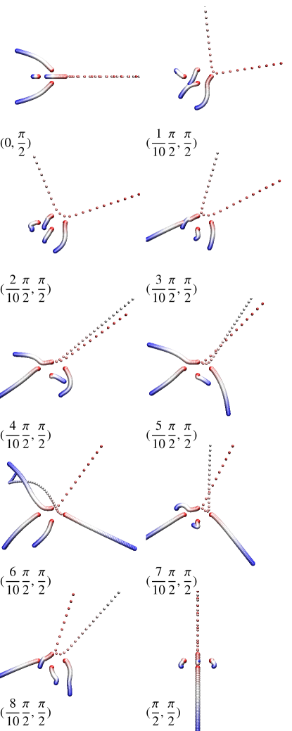
Figure 2: Scattering trajectories for various $(\phi,\theta)$ incidence angles. Atoms turn from red to white, and then to blue as time progresses. In this series, the $\theta$ angle is kept fixed at $\pi/2$.

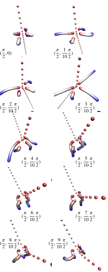
Figure 3: Scattering trajectories for various $(\phi,\theta)$ incidence angles. Atoms turn from red to white, and then to blue as time progresses. In this series, the $\phi$ angle is kept fixed at $\pi/2$.

An exhaustive study of this kind of collisions would require the systematic variation of the following initial conditions: the relative initial velocity of the colliding fragments, the vibrational state of the cluster, the incidence angles, and the impact parameter. Obviously, such a comprehensive study is out of the scope of any first principles methodology, and one must concentrate on a given parameter set and range. In this work, we concentrate on the incidence angles, since these are perhaps the variables whose small variations most easily produce different reaction outcomes.

We have simulated the collision of the proton with the lithium tetramer at a relative velocity of 0.02 a.u, which corresponds with a kinetic energy of 10 eV. This velocity was selected because it is sufficiently high to induce non-adiabatic effects (and indeed, we observed a small but non-negligible amount of ionization in most cases), but also not too high to induce too simple reactions: at higher velocities, we mainly observed “cluster transparency” (the proton passes through the cluster loosing part of its kinetic energy, but otherwise not altering its trajectory), followed in most cases by Coulomb explosion.

The proton is directed towards the center of the cluster (the impact parameter is therefore zero), and we have varied the incidence angles $(\phi,\theta)$ (see Fig. 1), in order to study how the change in the incidence angle modifies the possible reaction outcome. We have grouped the simulations in two groups: in the first group, we have studied in-plane collisions, fixing $\theta$ at $\pi/2$ and varying the $\phi$ angle. These are shown in Fig. 2. In the second group, shown in Fig. 3, the $\phi$ angle is fixed at $\phi=\pi/2$, and we varied $\theta$. Each collision event is represented on a single picture; the complete trajectory is shown by superimposing all the snapshots (taken at intervals of $\Delta t\approx 5~{}$fs), varying the color and tone of the atoms at different times to make the evolution evident.

In the first series, it can be seen how in all cases except one, the proton is scattered away at varying angles. For one case, however ($\phi=\frac{6}{10}\frac{\pi}{2}$), one of the Lithium atoms captures it, and a LiH molecule is formed. Interestingly, the Lithium that captures the proton is the first one to collide with the proton, but the capture happens only after the proton is scattered away also from a second proton. This demonstrates an important fact: in order for the proton to be captured by the cluster or by any of the resulting fragments, its energy must be low. A large incidence energy, however, deos not rule out the possibility of a capture, because the proton may loose energy if it is successively scattered by more than one atom. Other than the LiH, two Li atoms associate and form a dimer. In other trajectories of the first series, the Lithium atoms reorganize in different manners: for example, it is interesting to see how the $\phi=0$ collision results in Li₂ plus two free Lithium atoms, whereas the apparently similar $\phi=\pi/2$ case results in Li₃ plus only one Lithium atom. In the rest of the trajectories, the final configuration of positions (and velocities, which are not displayed) usually permits to predict what would be the final fragments. However, some cases are perhaps dubious, and longer simulation times would be needed.

In the second series (Fig. 3), the proton is scattered away in all cases. The reason is that the trajectories followed by the proton pass further away from any of the Lithium nuclei than in some of the in-plane cases. The first trajectory ($\theta=0$) is an example of cluster transparency: the trajectory of the proton is unaltered, and the Lithium tetramer, although highly excited both vibrationally and electronically, remains intact. For $\theta>0$, i.e., for non-orthogonal collisions, the proton leaves the cluster at a different angle. For $\theta\geq\frac{5}{10}\frac{\pi}{2}$, the Li₄ also retains its integrity, although strongly distorted. The other cases display different possible reaction channels.

In all these plots we have not shown the electronic cloud. As an example, we display in Fig. 4 six snapshots during the collision at $(\frac{6}{10}\frac{\pi}{2},\frac{\pi}{2})$ incidence angles. The analysis of the evolution of the charge may help to predict, at earlier times, whether or not two atoms are to remain associated: for example, the last snapshot (botton right) clearly shows the presence of charge between the two Lithium atoms on the left of the picture, and between the Lithium and the proton on top. This fact allows to infer with some confidence the formation of stable bonds (another possibility that would help in this task would be the use of the time-dependent electron localization function, which is also accessible with this methodology, see for example Ref. [31]).

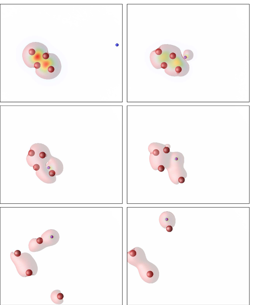
Figure 4: Six snapshot during the scattering trajectories for the $(\phi,\theta)=(\frac{6}{10}\frac{\pi}{2},\frac{\pi}{2})$ incidence angles. The snapshots correspond with the times $t=0$ (top left), $t=\frac{1}{6}T$ (top right), $t=\frac{2}{6}T$ (middle left), $t=\frac{3}{6}T$ (middle right), $t=\frac{4}{6}T$ (botton left) and $t=\frac{5}{6}T$ (botton right). $T\approx 200~{}$fs.

4 Conclusions

We have simulated the scattering of a proton with a lithium tetramer at moderate energies (10 eV), by making use of non-adibatic molecular dynamics based on TDDFT. An exhaustive analysis of this process would require a systematic variation of a large amount of initial conditions, such as the initial velocity of the colliding fragments, vibrational state of the target cluster or the impact parameter. This is unrealistic for any ab initio approach, but a careful selection of relevant parameters may provide interesting information: We have studied, for example, the different reaction channels that occur when the incidence angles of the proton change. Although long simulation times are needed in order to identify the final reaction products, these times are within the computational limits of the first principles approach that we have followed. In particular, we observed that for all the incidence angles considered the proton is scattered away, except in one interesting case in which one of the Lithium atoms captures it, forming a LiH molecule. In any case, the resulting collisions reveal interesting information about the scattered proton and the different reorganization of the Li fragments after the collisions, providing for each case self-explicative time-evolved trajectories. We conclude, therefore, that it is a suitable methodology to study the various reaction outcomes that result of proton-cluster collisions, or for any other non-adiabatic collisions in general.

References

- [1] Jörg Eichler, “Lectures on Ion-Atom Collisions”, (Elsevier, Amsterdam, 2005).
- [2] M. Nastasi, J. Mayer, and J. K. Hirvonen, “Ion-Solid Interactions: Fundamentals and Applications” (Cambridge University Press, Cambridge, 1996).
- [3] “Latest Advances in Atomic Cluster Collisions”, edited by Jean-Patrick Connerade and Andrey Solov’yov (Imperial College Press, London, 2004).
- [4] E. Runge and E. K. U. Gross, Phys. Rev. Lett. 52, 997 (1984).
- [5] “Time Dependent Density Functional Theory”, edited by M. A. L. Marques, C. A. Ullrich, F. Nogueira, A. Rubio, K. Burke, and E. K. U. Gross (Springer Verlag, Berlin, 2006).
- [6] J. Theilhaber, Phys. Rev. B 46, 12990 (1992).
- [7] U. Saalmann, and R. Schmidt, Z. Phys. D 38, 153 (1996).
- [8] E. K. U. Gross, J. F. Dobson, and M. Petersilka, in “Density Functional Theory” (Topics in Current Chemistry 181), edited by R. F. Nalewajski, p. 81 (Springer-Verlag, Berlin-Heidelberg, 1996).
- [9] T. Kunert, and R. Schmidt, Phys. Rev. Lett. 86, 5258 (2001).
- [10] U. Saalmann, and R. Schmidt, Phys. Rev. Lett. 80, 3213 (1998)
- [11] O. Knospe, J. Jellinek, U. Saalmann, and R. Schmidt, Eur. Phys. J. D 5, 1 (1999).
- [12] O. Knospe, J. Jellinek, U. Saalmann, and R. Schmidt, Phys. Rev. A 61, 022715 (2000).
- [13] M. Quijada, A. G. Borisov, I. Nagy, R. Díez Muiño, and P. M. Echenique, Phys. Rev. A 75, 042902 (2007).
- [14] M. Quijada, A. G. Borisov, and R. Díez Muiño, Phys. Stat. Sol. (a) 205, 1312 (2008).
- [15] J. M. Pruneda, D. Sánchez-Portal, A. Arnau, J. I. Juaristi, and E. Artacho, Phys. Rev. Lett. 99, 235501 (2007).
- [16] W. Zhi-Ping, W. Jing, Z. Feng-Shou, Chin. Phys. Lett. 27, 053401 (2010).
- [17] A. V. Krasheninnikov, Y. Miyamoto, and D. Tománek, Phys. Rev. Lett. 99, 016104 (2007).
- [18] Y. Miyamoto and H. Zhang, Phys. Rev. B 77, 161402(R) (2008).
- [19] A. Castro, M. A. L. Marques, J. A. Alonso, G. F. Bertsch, and Angel Rubio, Eur. Phys. J. D 28, 211 (2004).
- [20] T. Kunert, F. Grossmann, and R. Schmidt, Phys. Rev. A 72, 023422 (2005).
- [21] T. Fennel, K.-H. Meiwes-Broer, and J. Tiggesbäumker, Rev. Mod. Phys. 82, 1793 (2010).
- [22] F. Calvayrac, P.-G. Reinhard, and E. Suraud, J. Phys. B: At. Mol. Opt. Phys. 31, 5023 (1998).
- [23] F. Calvayrac, P.-G. Reinhard, and E. Suraud, Eur. Phys. J. D 9, 389 (1999).
- [24] J. Handt, T. Kunert, and R. Schmidt, Chem. Phys. Lett. 428, 220 (2006).
- [25] E. Suraud, and P.-G- Reinhard, Phys. Rev. Lett. 85, 2296 (2000).
- [26] J. P. Perdew, and A. Zunger, Phys. Rev. B 23, 5048 (1981).
- [27] M. A. L. Marques, A. Castro, G. F. Bertsch, and A. Rubio, Comput. Phys. Comm. 151, 60 (2003). See also http://www.tddft.org/programs/octopus.
- [28] A. Castro, H. Appel, M. Oliveira, C. A. Rozzi, X. Andrade, F. Lorenzen, E. K. U. Gross, M. A. L. Marques and A. Rubio, Phys. Stat. Solidi B 243, 2465 (2006).
- [29] N. Troullier and J. L. Martins, Phys. Rev. B 43, 1993 (1991).
- [30] A. Castro, M. A. L. Marques, and A. Rubio, J. Chem. Phys. 121, 3425 (2004).
- [31] A. Castro, T. Burnus, M. A. L. Marques, and E. K. U. Gross, in “Analysis and Control of Ultrafast Photoinduced Reactions”, edited by O. Kühn and L. Wöste, Chapter 6.5, pp. 555-576 (Springer-Verlag, Heidelberg, 2007).