Event-driven simulations of a plastic, spiking neural network

Abstract

We consider a fully-connected network of leaky integrate-and-fire neurons with spike-timing-dependent plasticity. The plasticity is controlled by a parameter representing the expected weight of a synapse between neurons that are firing randomly with the same mean frequency. For low values of the plasticity parameter, the activities of the system are dominated by noise, while large values of the plasticity parameter lead to self-sustaining activity in the network. We perform event-driven simulations on finite-size networks with up to 128 neurons to find the stationary synaptic weight conformations for different values of the plasticity parameter. In both the low and high activity regimes, the synaptic weights are narrowly distributed around the plasticity parameter value consistent with the predictions of mean-field theory. However, the distribution broadens in the transition region between the two regimes, representing emergent network structures. Using a pseudophysical approach for visualization, we show that the emergent structures are of “path” or “hub” type, observed at different values of the plasticity parameter in the transition region.

I Introduction

Neurons can form plastic networks through connecting synapses with weights that are changed dynamically by the neural activity in the form of neural spikes. It has been established that the precise timing of these spikes determines whether and how the synaptic weights will be increased (potentiated) or decreased (depressed) abbott_synaptic_2000 ; van_rossum_stable_2000 ; roberts_spike_2002 ; dan_spike_2004 . With better understanding of spike-timing-dependent plasticity (STDP), it becomes increasingly important to find out its implications on the underlying network structure and, consequently, on the neural activity itself. Theoretical models of a plastic neural network typically consist of three components: neural dynamics, synaptic transmission, and network plasticity morrison_spike-timing-dependent_2007 ; chen_mean-field_2010 . As has been shown previously chen_mean-field_2010 , a simple self-consistent mean-field scheme can be constructed when these three ingredients of a plastic neural network are given. Reducing the neural and synaptic dynamics to a determination of response functions characterizing a mean-field medium, the network plasticity is left governed by one-dimensional random-walk dynamics. Such a mean-field scheme was applied chen_mean-field_2010 to a network of leaky integrate-and-fire neurons gerstner_spiking_2002 ; burkitt_review_2006 ; brette_exact_2006 , coupled through a jump-and-decay synaptic conductance dynamics tsodyks_synchrony_2000 , and under STDP rules van_rossum_stable_2000 , controlled by a plasticity parameter $w^{\star}$ representing the expected value of synaptic weights when firings of the neurons are purely driven by noise. While we do not expect that there is a broad range of cell types with different plasticity parameter values but otherwise similar physiological characteristics, different values of $w^{\star}$ can correspond to different stages of a (quasi-statically) growing and developing network. The mean-field theory (MFT) predicts a first-order phase transition and hysteresis from a low $w^{\star}$ regime of noise-driven activity to a high $w^{\star}$ regime of self-sustaining activity. It also predicts a narrow synaptic weight distribution as long as the overall rate of change of synaptic strength is low. In the current study, we perform intensive event-driven simulations brette_simulation_2007 on the same model network to compare with the predictions of MFT; the simulations also reveal emergent network dynamics and structures that are not captured by the MFT.

In Section II that follows, we briefly describe the simulated model of a plastic neural network, which was elaborated in our MFT study chen_mean-field_2010 . We then present in Section III the method and algorithm of the event-driven simulations used to explore the dynamics of the model. The results of the simulations for static uniform networks are reported in Section IV, where we present the mean activity levels for networks of different sizes as functions of synaptic input. These activity levels agree well with the MFT predictions in the stable phases of low and high activity but show a gradual increase in a transition region ($w_{1}^{\star}<w^{\star}<w_{2}^{\star}$, from the onset to the persistence of threshold firing events) instead of the sharp first-order jump predicted by MFT. We also analyze the sporadic patterns of self-sustaining threshold firings in the transition region to identify two types of threshold firing events. In Section V, we present simulation results with high resolution in the plasticity parameter $w^{\star}$ for a plastic network with $N=32$ neurons that has reached a stationary state of plasticity. The change in the synaptic-weight conformation of the network in the transition region manifests itself in the synaptic weight distribution, which is seen to broaden twice, along with a bimodal elevation of the average firing activity compared to that of a static network. To characterize the emergent synaptic-weight structure of the network in the transition region, we employ a pseudophysical approach for visualization in Section VI to generate a 2D layout of the network. Such an approach reveals a path or loop conformation near the lower end of the transition region ($w^{\star}\sim w_{1})$ for network sizes up to $N\approx 32$ and a hub conformation near the high end ($w^{\star}\sim w_{2}$) for $N\approx 24$ and greater. We then conclude and summarize our findings in Section VII.

II Model

While our method is applicable to other combinations of models of neurons, synapses and plasticity, we follow the same choices made in our mean-field approach chen_mean-field_2010 , which we describe briefly below.

In the integrate-and-fire model for the neurons, the state of a neuron $i$ is described by a membrane potential $V_{i}$, which follows the differential equation of a leaky integrator dayan_theoretical_2001

$$\tau_{m}\frac{dV_{i}}{dt}=V_{0}-V_{i}+G_{i}\left(\mathcal{R}-V_{i}\right),$$ (1)

where $\tau_{m}$ is the leak time for the membrane charge, $V_{0}$ is the resting potential when the neuron is in the quiescent state, and $\mathcal{R}$ is the reversal potential for the ion channels on the synapses. The total synaptic conductance $G_{i}$ for the neuron is given by the sum

$$G_{i}\equiv\sum_{j}w_{j,i}Y_{j}$$ (2)

over all presynaptic neurons, $j$. The synaptic weights $w_{j,i}$ define the network and the same active transmitter fraction $Y_{j}$ is assumed for all efferent synapses of neuron $j$. In addition to the continuous dynamics (1), a neuron fires when its membrane potential reaches a threshold value, $V_{\mathrm{th}}$. Then, its membrane potential drops immediately to a reset value, $V_{\mathrm{r}}$. The action potential of the integrate-and-fire model is assumed to be instantaneous and is not modeled explicitly. The spike train produced by the neuron $i$ is defined as the function

$$S_{i}\left(t\right)\equiv\sum_{n}\delta\left(t-t_{i,n}\right)$$ (3)

where $t_{i,n}$ is the time when the neuron $i$ fires for the $n$-th time.

The fraction $Y_{j}$ of the active transmitters is described by the Tsodyks–Uziel–Markram (TUM) model tsodyks_synchrony_2000 of neural transmission, where the transmitters are distributed in three states: “active”, with the fraction $Y$; “inactive”, with the fraction $Z$; and “ready-to-release”, with the fraction $X$. For efferent synapses of a presynaptic neuron $j$, these fractions follow the dynamics tsodyks_synchrony_2000

$$\frac{dX_{j}}{dt} = \frac{Z_{j}}{\tau_{R}}-uS_{j}X_{j}$$

$$\frac{dY_{j}}{dt} = -\frac{Y_{j}}{\tau_{D}}+uS_{j}X_{j}$$ (4)

$$\frac{dZ_{j}}{dt} = \frac{Y_{j}}{\tau_{D}}-\frac{Z_{j}}{\tau_{R}},$$

where $\tau_{D}$ is the decay time of active transmitters to the inactive state, $\tau_{R}$ is the recovery time for the inactive transmitters to the ready-to-release state, and $u$ is the fraction of ready-to-release transmitters that is released to the active state by each presynaptic spike. With the conservation rule

$$X_{j}+Y_{j}+Z_{j}=1,$$ (5)

there are two independent variables per presynaptic neuron. Consistent with the TUM dynamics, the values of the factors multiplying $S_{j}$ at the discontinuities are to be evaluated immediately before the discontinuities.

While the integrate-and-fire and TUM dynamics are both deterministic, we model the stochasticity of the network with additional noise-driven firing events following Poisson statistics with the frequency $\lambda_{N}$ for each neuron. The noise-driven firings are treated the same way as threshold firings, that is, the membrane potentials are brought instantaneously to the reset value $V_{\mathrm{r}}$ and the firing times are included in the spike trains (3) of the transmitter dynamics (4).

To minimize the computational cost, the active transmitter fractions $Y_{j}$ double as the exponentially decaying “window functions” in our version of the plasticity rules suggested by van Rossum et al. van_rossum_stable_2000 . The synaptic weights are taken to follow the dynamical equation

$$\frac{dw_{j,i}}{dt}=\Delta Y_{j}S_{i}-rw_{j,i}Y_{i}S_{j}$$ (6)

where $\Delta$ is the parameter for additive potentiation and $r$ is the parameter for multiplicative depression. We define the plasticity parameter as the ratio

$$w^{\star}\equiv\frac{\Delta}{r},$$ (7)

which is equal to the expectation value of the synaptic weight when we have the symmetry $\left\langle Y_{j}S_{i}\right\rangle=\left\langle Y_{i}S_{j}\right\rangle$, e.g., when $S_{i}$ and $S_{j}$ are both Poisson spike trains of the same frequency. Fixing $w^{\star}$ leaves the depression factor $r$ as an overall control parameter for the rate of plasticity.

Table 1: Values of parameters used in calculations

integrate and fire				TUM model
resting potential $V_{0}$:	-55 mV			decay time $\tau_{D}$:	20 ms
leak time $\tau_{m}$:	20 ms			recovery time $\tau_{R}$:	200 ms
firing threshold $V_{\mathrm{th}}$:	-54 mV			release fraction $u$:	0.5
reset potential $V_{\mathrm{r}}$:	-80 mV			noise frequency $\lambda_{N}$:	1 Hz
reversal potential $\mathcal{R}$:	0 mV			plasticity rate $r$:	0.01

It is common for a model of a biological system to carry a large number of empirical parameters. Instead of exploring all possible ranges of these parameters, we fix them with physiologically plausible values that are commonly found in the literature. Unless otherwise stated, the values of the parameters are as listed in Table 1.

III Simulation Method

The disparity between the time scales of spiking activities and neural plasticity posts a significant challenge to computer simulations of plastic neural networks. Particularly for STDP, where precise timing is crucial in determining synaptic changes, we can not alleviate the computation requirement through use of larger integration time steps. However, for continuous dynamics that can be solved analytically, one can improve the efficiency of computation through an event-driven approach similar to that described by Brette brette_exact_2006 , which gives machine precision timing for the spikes and requires limited amount of computation upon each spike production.

In the event-driven approach, instead of calculating the state of the system for a fixed increment of time, one calculates the time for the next discontinuous event. This approach is feasible when the continuous dynamics of the system is solvable so that the time for the next discontinuous event can be evaluated efficiently. For the leaky integrate-and-fire model considered, an analytical form can be written down for the trajectory of the normalized membrane potential brette_exact_2006

$$v_{i}\equiv\frac{V_{i}-V_{0}}{\mathcal{R}-V_{0}}=xe^{x}\left[E_{1}\left(x\right)-E_{1}\left(G\right)+\frac{v}{Ge^{G}}\right]$$ (8)

where $E_{1}$ is the exponential integral function of the first kind, $x\equiv Ge^{-t/\tau_{m}}$, and $v=v_{i}\left(0\right)$, $G=G_{i}\left(0\right)$ are the initial states of the neuron. For the TUM dynamics, the transmitter fractions follow the trajectories

$$Y_{i} = e^{-t/\tau_{D}}Y$$

$$Z_{i} = \left[Z+\frac{\tau_{R}}{\tau_{R}-\tau_{D}}Y\right]e^{-t/\tau_{R}}-\frac{\tau_{R}}{\tau_{R}-\tau_{D}}Y_{i}$$ (9)

where $Y=Y_{i}\left(0\right)$ and $Z=Z_{i}\left(0\right)$ are their initial values. With the trajectory (8), one can solve for the time of the next threshold crossing $V_{i}\rightarrow V_{\mathrm{th}}$ through, e.g., a root solver. The computation time for a root solver to find the position of the crossing depends only logarithmically on the precision required, compared to the linear increase for the fixed-time-step approach. Further improvement of the computational efficiency can be achieved by, e.g., precomputing a lookup table for the time to threshold crossing given the current state of a neuron and interpolating when the desired value falls between precomputed points. For the simulated network with Poisson noise, the algorithm is as outlined below:

1. For each neuron $i$ in the system, calculate the time-to-fire $t_{\mathrm{ttf}}^{i}$ from the continuous, deterministic dynamics of the model.

2. Draw the time to its next noise-triggered firing $t_{N}^{i}$ from an exponential distribution with the expectation value $\lambda_{N}^{-1}$ for each neuron $i$.

3. Find the minimum of the times $t_{\mathrm{ttf}}^{i}$ and $t_{N}^{i}$ among all neurons to be the time to the next discrete event $\Delta t$ of the system.

4. Advance the simulated clock by $\Delta t$ and update the state of the system using Eqs. (8) and (9).

5. Fire the selected neuron $i$ by reseting its membrane potential to $V_{i}=V_{R}$, and increasing the affected active transmitter fraction $Y_{i}$ by $u\left(1-Y_{i}-Z_{i}\right)$.

6. Repeat this process from 1.

For the current model, the simulated dynamics boils down to the evaluation of the time-to-fire $t_{\mathrm{ttf}}\left(V,G\right)$ given the initial membrane potential $V$ and total synaptic conductance $G$ as well as the evaluation of the trajectories (8) and (9). We note that instead of the common approach of defining the model with the set of differential equations (1) and (4), it is equally valid and computationally preferable to define the continuous dynamics of the model with the trajectories (8) and (9) for the neurons and synapses.

IV Static network

Before incorporating plasticity, we first perform event-driven simulations on fully-connected networks of up to 128 neurons with uniform, fixed synaptic weights $w$. This exercise will prepare us for the inclusion of plasticity and also reveal the emergence of “structure” in the network. The average activity levels for different system sizes are shown in Fig. 1

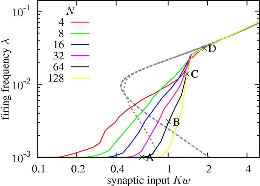
Figure 1: (Color online) Mean activity level vs. total synaptic input ($Kw$) for fully-connected uniform networks (node degree $K=N-1$) with static synaptic weight ($w$). Dashed lines are predictions from mean-field theory without fluctuation corrections (long dashes) and with the inclusion of shot-noise-like fluctuations (short dashes) in total synaptic conductance for a network with $K=63$ afferent synapses per neuron.

compared with predictions from MFT chen_mean-field_2010 . As expected, the average activity levels of the simulated network coincide with mean-field predictions in the stable phases of low and high activity. However, in the transition region between the two phases, the activity levels from network simulations increase continuously instead of exhibiting the jumps and hysteresis predicted by mean-field theory. We note that the hysteresis in MFT chen_mean-field_2010 comes about when there are two stable states in the system: a quiet state with only noise-triggered firings that are insufficient to ignite the entire system, and an active state in which firings are system-wide and self-sustaining. However, for a finite-size network having sufficient fluctuations and running for a sufficient time, the system can make transitions between the two states, leading to a single-valued mean activity level of the system showing no hysteresis. Comparing networks of different sizes, the rise of the average firing frequency in the transition region is steeper for larger networks since fluctuations in the total synaptic conductance decrease with an increase in the number of afferent synapses chen_mean-field_2010 rendering mean-field theory a better approximation.

The firing pattern of the $N=64$ network is shown in Fig. 2 for 4 different values of synaptic input $Kw$ as marked in Fig. 1.

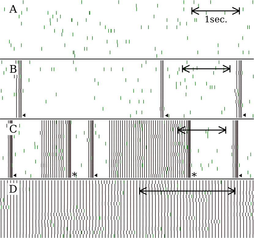
Figure 2: (Color online) Firing polygraphs of the $N=64$ network at 4 different values of synaptic strength $w$ labeled in Fig. 1. For each value, only activities of 16 randomly chosen neurons are shown, with each occupying 1/16 of the height of the corresponding strip. The light and dark vertical line segments mark the firings due to noise and threshold crossing, respectively. The time on each strip of recording runs towards the left with a scale indicated by the one second time interval on each strip. Symbols ($\blacktriangleleft$ and $\ast$) mark clusters of threshold firings as detailed in text.

With computer simulations, we are able to distinguish firings due to threshold crossings of the membrane potentials (marked with dark vertical line segments) from noise triggered firings (marked with light vertical line segments). We can thus define a system to be active when there is any neuron with a membrane potential set to cross the firing threshold without the help of further noise events. Operationally, this is when the time-to-fire $t_{\mathrm{ttf}}^{i}$ calculated in step 1 of the event-driven algorithm 1 is finite for any of the neurons. The switching between the quiet and active states of the network are evident on the strips B and C. This leads to clusters of threshold firings during which the system remains active. In the specific model we considered, there are two types of threshold firings clusters that can be identified from the polygraphs. The first represents bursting, which are brief clusters (up to a few hundred milliseconds) of threshold firings of generally similar durations. These can be seen for all threshold activities on strip B and some on strip C as marked by the symbol “$\blacktriangleleft$” in Fig. 2. The second type of threshold firing activity is intermittently persisting activity, that can last for seconds, are of a wider range of durations and are seen in two time segments marked by the symbol “$\ast$” on strip C of Fig. 2. The two types of clusters of threshold firings can also be identified from the duration distribution of self-sustained threshold firings shown in Fig. 3.

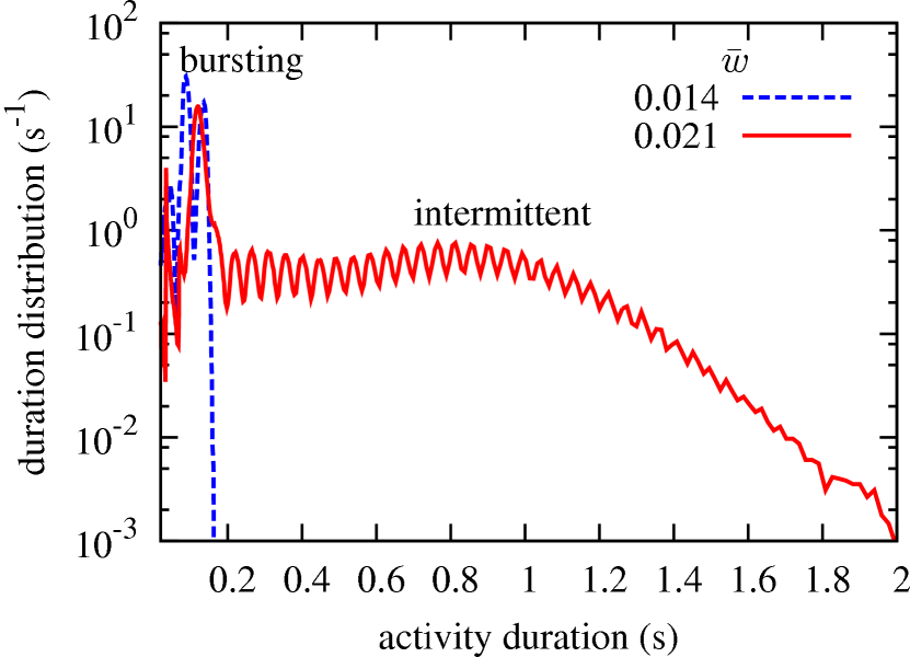
Figure 3: (Color online) Time-weighted duration distribution of sustaining threshold firing activities. The system is considered active when any of the neurons is set to cross the firing threshold without further noise events. The duration is measured for each episode of the system staying continuously active. The oscillations in the distribution comes from the periodic nature of persistent firing activities. Values of the synaptic weight $\bar{w}$ (0.014, dashed line and 0.021, solid line) correspond to the locations B and C, respectively in Figs. 1 and 2.

The distinction between the two kinds of activities can be attributed to the short-term depression caused by the inactive state of synaptic transmitters in the TUM model: When threshold firings of the network are just ignited after a quiet period, most transmitters are in the ready-to-release state and activities can propagate easily leading to a somewhat higher firing rate of the neurons in the beginning. However, as most transmitters are deposited into the inactive state during repeated firings, the firing frequency is reduced. At the low activity end of the transition region, the reduction of firing frequency typically continues all the way to a cessation of any threshold firings, leading to the short bursting events of similar duration. Near the high activity end of the transition region, as the transmitters become inactive, the reduced firing frequency can settle to a stable value that can last for seconds before all threshold firings stop.

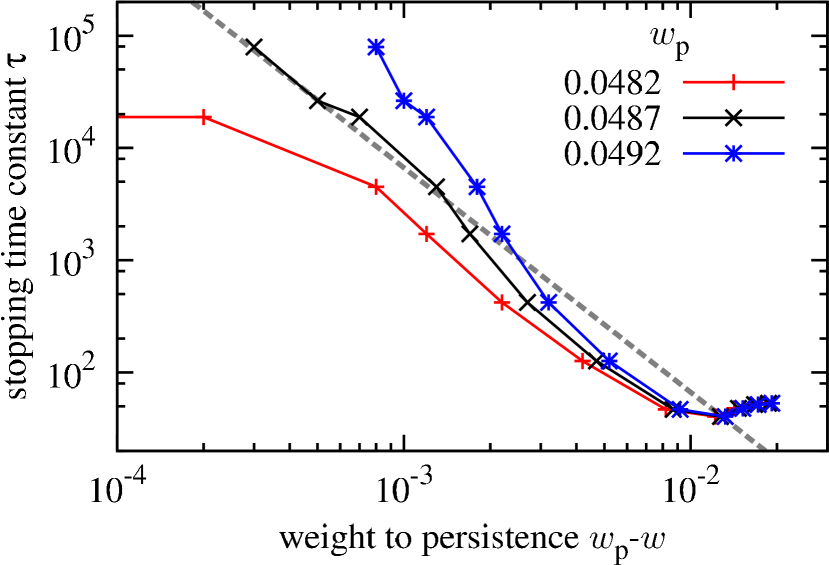
Figure 4: (Color online) Scaling of “stopping time constant” estimated from the tail of active duration distribution in Fig. 3 for a $N=32$ static uniform network. The best estimate of $w_{\mathrm{p}}=0.0487$ for the diverging point (center curve) is shown along with two slight deviations. The dashed line is to show the estimated slope of -2 for comparison.

From the simulation results such as what are shown in Fig. 3, the stopping of the threshold firings seem to follow Poisson statistics, that is, it can be characterized by a stopping rate $\tau^{-1}$. The duration distribution of sustaining threshold firings decays exponentially for large duration with the time constant $\tau$ that increases with $w$ and appears to diverge at some $w=w_{\mathrm{p}}$. For the $N=32$ network, we estimate $w_{\mathrm{p}}\approx 0.0487$ and that the “stopping time constant” diverges roughly with the scaling $\tau\sim\left(w_{\mathrm{p}}-w\right)^{-2}$ as suggested in Fig. 4. We note that the scaling form of the stopping time remains the same when we simplify the TUM dynamics in our model by removing the inactive state (data not included here), suggesting at least some degree of universality. These results suggest that the divergence of the stopping time constant $\tau$ signals that the system enters the phase of truly self-sustaining activity.

V Dynamic (Plastic) network

For the current study, we focus on the stationary states of the system under the plasticity dynamics. A uniform network with synaptic weight $w_{j,i}=w^{\star}$ for all synapses is used as the initial configuration, and simulations are conducted at each data point for at least $2^{31}$ ms ($\approx 25$ days) of simulated time to reach the stationary state. We concentrate our calculations on a fully-connected network of $N=32$ neurons with a high resolution in the plasticity parameter $w^{\star}$. For each $w^{\star}$, all measurements are averaged over an ensemble of 32 or more independent runs of different random sequences.

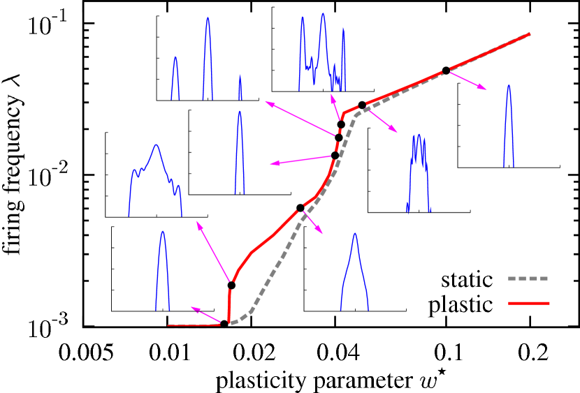
Figure 5: (Color online) Activity–plasticity(parameter) plot for a fully connected plastic network of $N=32$ neurons compared with the activity level of a static network of the same size with uniform weight $w=w^{\star}$. The plastic network is allowed to reach a stationary state by running for about 25 days of simulated time. All results are averaged over an ensemble of 32 or more runs of different random sequences. Insets of the plot show the normalized synaptic weight distributions on a log-log scale with a range of 2 (4) decades on the horizontal (vertical) axis at different points marked on the activity–plasticity curve.

The results of the calculations are summarized in Fig. 5, where we see that the firing frequency of a stationary plastic network coincides with that of a uniform static network ($w=w^{\star}$ for all synapses) in the low-activity, noise-dominated regime as well as in the persistently active regime. In the transition region between the noise-driven and self-sustaining regimes, the firing rate of the network is enhanced by the plasticity, and, while the behavior is not universal, with TUM synapses the amount of enhancement exhibits an interesting bimodal shape.

In the insets of Fig. 5, we show the synaptic weight distribution, also averaged over the same ensemble, at each marked point along the activity–plasticity curve. In the two stable regimes, noise-dominated and persistently-active, the synaptic weights have a Gaussian distribution with a narrow width (within about 5% of $w^{\star}$) as predicted by MFT chen_mean-field_2010 . However, coincident with the bimodal enhancement of firing frequency, the synaptic weight distribution of the stationary plastic network shows dramatic changes in the transition region along the activity–plasticity curve: Increasing the plasticity parameter $w^{\star}$ from the noise-dominated low-activity regime, we see a discontinuous jump in the firing rate and sudden broadening of the weight distribution with tiered side peaks at $w^{\star}\approx 0.017$. The enhanced firing and broadened distribution ease off after the jump, until these features become insignificant around $w^{\star}=0.04$. At this point, with a slight increase of $w^{\star}$, two disconnected side peaks pop out in the synaptic weight distribution. However, such a splitting in the weight distribution is only accompanied by a gradual enhancement of average firing rate of the plastic network. The two side peaks eventually merge back to the main peak with further increases of $w^{\star}$. This eventually returns the network to a uniform conformation with a narrow Gaussian synaptic-weight distribution before the plasticity parameter reaches $w^{\star}\simeq 0.1$.

Instead of a simple increase of the Gaussian width, the observed broadening of the synaptic weight distribution in the transition region just summarized (see Fig. 5) comes with structured side peaks, which signify emergent network conformations that we try to decipher and visualize with a pseudophysical approach in Section VI. For the $N=32$ and smaller networks, we are able to obtain a stationary state from the simulation run that is insensitive to the initial configuration at each data point (value of $w^{*}$). However, we do see runaway synaptic weights under the plasticity rules used for the $N=48$ and $N=64$ networks in narrow, isolated intervals at $w^{\star}\approx 0.0268$ and $w^{\star}\approx 0.0194$ respectively near the high-activity end of the transition region before the runs ($2^{31}$ms, $\sim$25 days, of simulated time) are complete. For these instances, the diverging synaptic weights and firing frequencies of the driven neurons slow the simulation down to a near standstill, and we can not always maintain a stationary system as we vary the plasticity parameter across the runaway point. We note that such runaways are commonly seen in models with Hebbian plasticity and are typically “cured” with cutoffs in the range of synaptic weights. amarasingham_predictingdistribution_1998 ; song_competitive_2000 ; rubin_equilibrium_2001 ; toyoizumi_optimality_2007 We do not need such a device for the $N=32$ network results presented. For larger networks, when we do see such “isolated” runaways, we regard them as pathological hasselmo_runaway_1994 ; greenstein-messica_synaptic_2011 and exclude them from the ensembles.

VI Network “Layout”

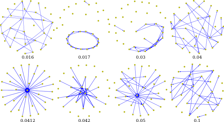
Figure 6: (Color online) Typical resultant layouts of neurons (represented by the dots) following the pseudophysical approach described in the text at the points marked on the activity–connectivity curve in Fig. 5. The number labeled below each layout is the corresponding value of the plasticity parameter $w^{\star}$. Only the strongest 31 synaptic connections (lines with arrows) are shown in each layout.

Characterizing the structure of non-uniform networks is an active field of research bullmore_complex_2009 ; boccaletti_complex_2006 ; newman_modularity_2006 . Here we adopt a more intuitive and visual approach to extract any emergent structures of the stationary plastic network obtained above. Under our model setup, such structures reside in the framework of a fully-connected network of uniform connectivity, represented by the main peak in the synaptic weight distribution. In this section, we attempt to uncover the topological meaning of the side peaks seen for the distribution in the transition region between the two stable phases of the system.

In order to visualize the networks such that any emerging features can be better revealed, we introduce a pseudophysical system of fictitious interacting particles in two dimensions representing the neurons, recognizing, of course, that the actual all-to-all network is not strictly two-dimensional. The nodes (pseudo particles) are imagined to be located on the plane, confined to the region near an arbitrary origin by an isotropic harmonic potential. The nodes interact with a (fictitious) pair-wise repulsive force that is determined by the synaptic weights between the neurons. To have the pseudo-particles representing neurons that are more strongly connected stay close to one another, we choose a repulsive pairwise force

$$\vec{F}_{i,j}=\frac{\hat{e}_{j,i}}{w_{i,j}^{2}+w_{j,i}^{2}}$$ (10)

to act on particle $i$ due to $j$ with $\hat{e}_{j,i}=\vec{r}_{j,i}/\left|\vec{r}_{j,i}\right|$ being the unit vector along the $\vec{r}_{j,i}=\vec{r}_{i}-\vec{r}_{j}$ direction (in the two-dimensional pseudo-space). In fitting the entire layout of the pseudo-particles (representing neurons) to a fixed display area, the strength $k$ of the confining harmonic potential is adjusted so that, in an equilibrium arrangement of the particles, the radial coordinate $\vec{r}$ of the particle farthest from the origin of the potential has magnitude equal to $1$. Such a pseudophysical system of neurons is relaxed to reach a stable arrangement of neurons in which the net force on each pseudo particle (neuron) is zero. The relaxation is accomplished through a deterministic, over-damped dynamics in which the velocity of each node is proportional to the net force it experiences

$$\frac{d\vec{r}_{i}}{dt}=-k\vec{r}_{i}+\sum_{j}\vec{F}_{i,j}.$$ (11)

The representative layouts for the marked data points in Fig. 5 are shown in Fig. 6, where we only show a fraction of the synapses with strongest weights along with the pseudo-positions to reduce obscurity. We note that the stable layouts reached are not unique for the system, and it is possible for the pseudo-particle system to be trapped in a metastable configuration in which strongly connected neurons are hindered by other neurons and fail to get close to each other during the relaxation. We do not attempt to further relax the layout (by, e.g., perturbing the positions of the neurons) after a stable configuration is reached during the relaxation process. (We note that for larger systems where the “hindrance” can be more severe, one may consider a three or higher dimensional pseudophysical system to help alleviate the problem.)

As revealed in layouts of Fig. 6, the jump in the firing rate near $w^{\star}=0.017$ is accompanied by the formation of a path conformation in the network where synapses of stronger synaptic weights connect a sequence of neurons and facilitate the propagation of activities along the path. Such a path can form a closed loop near the jump but become less likely to do so as $w^{\star}$ is increased. The path or loop structure is stable in the system such that once it forms, it will generally remain to the end of our simulation run at a fixed $w^{\star}$ value. As we only present results of simulations from uniform initial networks, there is no hysteresis loop in Fig. 5. However, the jump in the firing rate signals a first-order phase transition. While we have not attempted a systematic study of hysteresis effects with larger systems, we do see some degree of hysteresis in smaller ($N\leq 16$) networks: If we use a loop conformation obtained in the stationary state of the network at a $w^{\star}$ value above the jump as the initial condition for the simulation of the network at a $w^{\star}$ value below the jump, the loop conformation can sometimes persist over the course of the entire simulation. With a path or loop conformation of the network, the tiered side peaks of the synaptic weight distribution in this area come from the skip-over synapses along the path, i.e., synapses that are along the direction of the path but bypass some of the neurons.

Eventually, with the increase of $w^{\star}$, the path falls apart and the network returns to a uniform conformation around $w^{\star}=0.04$. The emergence of disjoint side peaks in the synaptic weight distribution with a slight increase of $w^{\star}$ from $0.04$ as seen in Fig. 5 is accompanied by the formation of a sink hub structure in the network where the high activity level of the hub neuron and its strong afferent synapses reinforce each other because of the positive-feedback nature of the synaptic plasticity. This type of hub structure is first seen at $w^{\star}=0.0411$ in our simulations and can go in and out of existence several times during the course of our simulation run at a fixed $w^{\star}$. This partially explains why we only see a gradual increase of the average activity level when a hub start to form. The sink hub structure becomes more and more stable as $w^{\star}$ increases until multiple hubs appear in the network around $w^{\star}=0.0414$. The network returns to a uniform conformation through the increasing number of less and less significant hubs. Finally, at sufficiently large $w^{\star}$ the network has reached a homogeneous, high-activity state.

We can now try to understand the formation of “path” and “hub” conformations in different segments of the transition region separating homogeneous, stable low- and high-activity states of the network. Near the low-activity end of the transition region, the sequence of neurons along the path represents a firing order in a bout of threshold firings that is amplified and preserved by the STDP as the path of stronger synaptic weights. Especially when such a path forms a loop, threshold firing activity can cycle through all neurons in the loop no matter which one of them is triggered by the noise. However, near the high-activity regime, each neuron generally fires multiple times during an episode of sustaining threshold firings with a high frequency. The firing order of neurons loses its meaning because there are many ways of pairing up their spikes. In this area of the transition region, the main distinguishable feature of a neuron is simply its firing rate. In fact, the expectation value of a synaptic weight $w$ for a synapse in this range can be uniquely determined from the firing rates of its pre- and postsynaptic neurons when the firing rates of the neurons are high enough ($\lambda>\tau_{D}^{-1},\tau_{m}^{-1}$) so that the actual timing of spikes becomes unimportant. Under such a condition, the stationary synaptic weight under the plasticity dynamics (6) for, say, the $j\rightarrow i$ synapse, is given by

$$w_{j,i}=w^{\star}\frac{\bar{Y}_{j}\lambda_{i}}{\bar{Y}_{i}\lambda_{j}}$$ (12)

where $\bar{Y}_{i}\equiv\left\langle Y_{i}\right\rangle$ and $\lambda_{i}\equiv\left\langle S_{i}\right\rangle$ are, respectively, the average active transmitter fraction and mean firing rate of the neuron $i.$ With Eq. (12), the condition

$$w_{i,j}w_{j,k}w_{k,i}=w^{\star 3}$$ (13)

should hold for any neurons $i\neq j\neq k$ in the network . And, indeed, we have verified that the condition (13) is well satisfied by the hub conformations obtained in the simulations, but is apparently violated by the path conformations (data analysis not presented here).

While it is tempting to correlate the layouts resulting from our pseudophysical arrangement with configurations of physical neurons, we must caution that one can only view such a pseudophysical approach as an arbitrary and non-unique way of revealing network structures. Furthermore, the structures found by the pseudophysical approach do not represent any direct physical information contained in the parameters of the neuron network. Nonetheless, it helps to provide an intuitive “structural” understanding of the network conformation as we have shown above.

VII Conclusions

The event-driven algorithm presented in Sec. III improves the accuracy and efficiency of the simulations allowing us to gain an intensive view of the phase space of a stationary plastic neural network. With a large number of parameters typical for a model of a biological system, we fix all but one, the plasticity parameter, with physiologically plausible values for our investigation. Also, to minimize conceptual complications, we study only the stationary properties of fully-connected networks driven by uniform, non-correlated Poisson noise. Our results show the network develops interesting structures in the transition region between the stable phases corresponding to low- and high-activity regimes. While our fully-connected network with a limited number of neurons is certainly inadequate to address the dynamics of a real brain, it can be a reasonable starting point for cultured networks consisting of hundreds of neurons with virtually “all-to-all” interactions bi_synaptic_1998 ; segev_observations_2001 ; shefi_morphological_2002 ; beggs_neuronal_2003 ; lai_growth_2006 . Our finding suggests that emergent structures in these networks are more likely to be seen when it is firing intermittently in the transition region perhaps during its development from a weakly-coupled system of neurons to a more strongly connected network.

The characterization of network connectivity is an active field of research with established quantifications such as the “clustering coefficient” barrat_architecture_2004 and “modularity” newman_modularity_2006 . However, in the current study, we adopt a simple visualization approach to gain a more intuitive view of the network structure. The resultant identification of the “path” and “hub” conformations explains or, more accurately, coincides, with the appearance of structured side peaks in the synaptic weight distribution and the elevated firing rate of the neurons. While these path and hub conformations are the simplest forms that can appear in a connected network, the present work is the first to demonstrate that they can arise naturally in transition regions of a neural network under STDP and driven only by noise. The connection-weight conformation (i.e., the distribution and correlations of synaptic weights) of a naturally occurring network is often strongly influenced by activity during its formation and maturation. However, studies of network dynamics typically focus on behavior of the network under given, static network topology or weight conformation. Advances in the understanding of the network plasticity are setting the stage for addressing how the observed conformation of these networks can come about. Our study of a pure and simple network is just an initial step along this direction, and it leaves open questions of how variations of biological details that are fixed in our model and different network topology, geometry, or sparseness might affect the emergent structures and alter the dynamical behavior of the network.

In addition, there remain pronounced and puzzling features observed in the current study that require further elucidation. For example, while both types of conformations (hubs and paths) appear abruptly as the plasticity parameter $w^{\star}$ is varied, the average firing rate increases with a discontinuous jump for the path conformation, but continuously for the hub. Also, the system does not “morph” from the path conformation to the hub conformation directly but, instead, returns to a uniform network before developing the hub structure. This feature might suggest a symmetry or “topological” difference between the two types of conformations that prevents a direct transition from one conformation to the other.

Finally, while we have only considered a stationary network driven by uncorrelated noise, arguably the ultimate “goal” of a plastic neural network is learning to serve specific or varying functional requirements. On this regard, it will be of great interest to subject the system to more meaningful inputs and explore the change in the stationary structures as well as the transient dynamics of the resultant network.

- (1) L. F. Abbott and S. B. Nelson, Nature Neuroscience 3, 1178 (2000)
- (2) M. C. W. van Rossum, G. Q. Bi, and G. G. Turrigiano, Journal of Neuroscience 20, 8812 (Dec. 2000)
- (3) P. D. Roberts and C. C. Bell, Biological Cybernetics 87, 392 (Dec. 2002)
- (4) Y. Dan and M.-M. Poo, Neuron 44, 23 (Sep. 2004), ISSN 0896-6273
- (5) A. Morrison, A. Aertsen, and M. Diesmann, Neural Computation 19, 1437 (Jun. 2007)
- (6) C.-C. Chen and D. Jasnow, Physical Review E 81, 011907 (2010)
- (7) W. Gerstner and W. M. Kistler, Spiking Neuron Models: Single Neurons, Populations, Plasticity (Cambridge University Press, 2002) ISBN 0521890799
- (8) A. Burkitt, Biological Cybernetics 95, 97 (2006)
- (9) R. Brette, Neural Computation 18, 2004 (2006)
- (10) M. Tsodyks, A. Uziel, and H. Markram, Journal of Neuroscience 20, RC50 (2000)
- (11) R. Brette, M. Rudolph, T. Carnevale, M. Hines, D. Beeman, J. Bower, M. Diesmann, A. Morrison, P. Goodman, F. Harris, M. Zirpe, T. Natschläger, D. Pecevski, B. Ermentrout, M. Djurfeldt, A. Lansner, O. Rochel, T. Vieville, E. Muller, A. Davison, S. E. Boustani, and A. Destexhe, Journal of Computational Neuroscience 23, 349 (Dec. 2007)
- (12) P. Dayan and L. F. Abbott, Theoretical Neuroscience: Computational and Mathematical Modeling of Neural Systems (Massachusetts Institute of Technology Press, Cambridge, Mass, 2001) ISBN 0262041995
- (13) A. Amarasingham and W. B. Levy, Neural Computation 10, 25 (1998)
- (14) S. Song, K. D. Miller, and L. F. Abbott, Nature Neuroscience 3, 919 (2000), ISSN 1097-6256
- (15) J. Rubin, D. D. Lee, and H. Sompolinsky, Physical Review Letters 86, 364 (2001)
- (16) T. Toyoizumi, J.-P. Pfister, K. Aihara, and W. Gerstner, Neural Computation 19, 639 (Mar. 2007)
- (17) M. E. Hasselmo, Neural Networks 7, 13 (1994), ISSN 0893-6080
- (18) A. Greenstein-Messica and E. Ruppin, Neural Computation 10, 451 (2011), ISSN 0899-7667
- (19) E. Bullmore and O. Sporns, Nature Reviews Neuroscience 10, 186 (Mar. 2009), ISSN 1471-003X
- (20) S. Boccaletti, V. Latora, Y. Moreno, M. Chavez, and D.-U. Hwang, Physics Reports 424, 175 (Feb. 2006)
- (21) M. E. J. Newman, Proceedings of the National Academy of Sciences 103, 8577 (Jun. 2006)
- (22) The loop product is an attempt to generalize the curl operator in metric spaces to a network. The condition (13\@@italiccorr) is equivalent to the curl-free condition of the “vector field” , which seems to hold in the hub conformations but not the loop or path conformations for the stationary plastic networks.
- (23) G.-Q. Bi and M.-M. Poo, Journal of Neuroscience 18, 10464 (Dec. 1998)
- (24) R. Segev, Y. Shapira, M. Benveniste, and E. Ben-Jacob, Physical Review E 64, 011920 (Jun. 2001)
- (25) O. Shefi, I. Golding, R. Segev, E. Ben-Jacob, and A. Ayali, Physical Review E 66, 021905 (2002)
- (26) J. M. Beggs and D. Plenz, J. Neurosci. 23, 11167 (Dec. 2003)
- (27) P.-Y. Lai, L. C. Jia, and C. K. Chan, Physical Review E 73, 051906 (May 2006)
- (28) A. Barrat, M. Barthelemy, R. Pastor-Satorras, and A. Vespignani, Proceedings of the National Academy of Sciences of the United States of America 101, 3747 (2004)