Scandalously Parallelizable Mesh Generation

Abstract

We propose a novel approach which employs random sampling to generate an accurate non-uniform mesh for numerically solving Partial Differential Equation Boundary Value Problems (PDE-BVP’s). From a uniform probability distribution $\mathcal{U}$ over a 1D domain, we sample $M$ discretizations of size $N$ where $M\gg N$. The statistical moments of the solutions to a given BVP on each of the $M$ ultra-sparse meshes provide insight into identifying highly accurate non-uniform meshes. Essentially, we use the pointwise mean and variance of the coarse-grid solutions to construct a mapping $Q(x)$ from uniformly to non-uniformly spaced mesh-points. The error convergence properties of the approximate solution to the PDE-BVP on the non-uniform mesh are superior to a uniform mesh for a certain class of BVP’s. In particular, the method works well for BVP’s with locally non-smooth solutions. We present a framework for studying the sampled sparse-mesh solutions and provide numerical evidence for the utility of this approach as applied to a set of example BVP’s. We conclude with a discussion of how the near-perfect paralellizability of our approach suggests that these strategies have the potential for highly efficient utilization of massively parallel multi-core technologies such as General Purpose Graphics Processing Units (GPGPU’s). We believe that the proposed algorithm is beyond embarrassingly parallel; implementing it on anything but a massively multi-core architecture would be scandalous.

1 Introduction

A wide range of linear and non-linear boundary value problems, such as the Poisson, Helmholtz, and non-linear Poisson-Boltzmann equations, arise in protein folding, molecular dynamics, neutral and non-neutral plasmas, acoustics and antenna design, etc. In many of these applications, sparse mesh-points are sufficient over vast regions of the domain, while large, iterative, and parallel computations using a high density of points are necessary for obtaining accuracy in the vicinity of complex objects. In this paper, we propose a novel approach for generating mesh-points to be used in simulating solutions to Boundary Value Problems (BVP). The class of methods is designed to discover accurate non-uniform discretizations via a sparse stochastic approximation.

State of the Art numerical methods typically have some mechanism for refining the underlying mesh. At some level, all adaptive methods are attempting to identify the optimal mesh, providing uniform accuracy over a given domain. Adaptive methods have been heavily employed in problems with complex geometry, where sharp geometric features can make the simulation difficult to resolve, or in simulations where shocks or discontinuities can arise over time.

Ideally, we would like an unstructured mesh that is designed to use coarse resolution where the solution changes little, and fine resolution where transitions take place, such as near a boundary. This is not a new idea, as this is the guiding principle in deciding where to apply Adaptive Mesh Refinement (AMR) for Hyperbolic conservation laws. Recent work in Hyperbolic conservation laws has gone as far as developing metrics to guide refinement which are based on an estimated error between the numerical solution and the weak solution [14, 15]. Like with hyperbolic problems, the idea of working on the smallest mesh possible while maintaining a uniform accuracy is not a new topic when it comes to the area of numerical boundary value problems. For boundary value problems with Lipschitz sources there are a range of methods which can be employed to increase accuracy at boundaries where there are transitions. One of the simplest is to make use of Chebyshev points, which pack resolution near boundaries and still allow one to construct high order approximate inverse operators [2]. However, in a wide range of nonlinear boundary value problems, there are interesting issues which arise, including the formation of interior layers or singularities at unknown locations. In 1D, if one knew where a transition layer or singularity is located, one could design Chebyshev points to increase resolution nearby. Unfortunately, it may be non-trivial to identify the transition layer or develop an efficient implementation in higher dimensions.

Quasi Monte Carlo and low discrepancy sequences offer an alternative approach to sparse mesh theory [4, 19, 20]. A Monte Carlo method is a statistical approach to compute the volume of a complex domain in high dimensions. Briefly, given a complex domain, $D_{c}$, one encompasses the domain in a simple region $D$ and then points are sampled from $D$ and tested to see whether they lie inside of $D_{c}$. The fraction of the points from $D$ that lie inside $D_{c}$ are used to estimate the volume of domain $D_{c}$. As the number of samples, $N$, go to infinity, it is well known that this method converges at a rate of $\mathcal{O}(\sqrt{N})$. A quasi-Monte Carlo method is formulated in the same way, except that instead of using randomly generated points, a pre-determined set of points, called a low-discrepancy sequence, is used in the estimation of the volume $D_{c}$ [12]. The Quasi Monte Carlo method converges at a rate of $\mathcal{O}(N)$. If one views a PDE from a numerical Green’s function formulation, low-discrepancy sequences are one approach to numerically computing a solution in complex domains. These methods have been used in the solution of integral equations [6, 7], and more recently, in the solution of PDE’s [7]. The basic premise is that a good estimate of the solution may be obtained with relatively few samples, i.e., a sparse mesh.

Our proposed strategy differs from all the above frameworks in that it uses sparse stochastic sampling to construct a non-uniform mesh-generation function $Q$. The approach is ideal for identifying the placement of mesh points to maintain uniform accuracy across the domain and is well suited to both finite difference and finite element formulations of a problem. Details of the approach and associated theoretical framework are described in Section 2 and include a preliminary investigation of convergence and well-posedness issues. Numerical examples are then presented in Section 3. Section 4 contains a summary of our results as well as a discussion of future directions. Lastly, since this work lies at the intersection of numerical PDE’s and statistics, some notation may be unfamiliar to some readers and accordingly, we include a glossary of notation in the Appendix.

2 Approach and Theoretical Framework

Non-uniform discretizations can offer superior solution accuracy and convergence properties. The challenge, however, lies in efficient identification of a mesh which provides results superior to that of uniform spacing. In this section, we offer a brief overview of our proposed algorithm as well as the establishment of a preliminary theoretical framework.

Consider a two-point Boundary Value Problem (BVP), e.g., the Poisson equation

$$u^{\prime\prime}(x)=f(x)\>\mbox{ s.t.}\, u(0)=A\,;\, u(1)=B\,,$$ (1)

for $A,B\in\mathbb{R}$ and $x\in\mathbf{I}=(0,1)$. Recall that a uniform discretization for the second derivative yields second-order convergence. We denote $\bar{\mathbf{I}}$ as the domain $[0,1]$, a discretization of the interior $\mathbf{I}$ as $\mathbf{x}_{n}=(x_{1},\ldots,x_{n})^{T}$, and the corresponding approximate solution at $\mathbf{x}_{n}$ as $\mathbf{u}_{n}=(u_{1},\ldots,u_{n})^{T}$. Note that frequently in the numerical analysis literature, the variables for spatial discretization and numerical solution are denoted by a superscript $n$. Here $n$ is a subscript, which is consistent with notation for random variables and will be used in this paper.

Next, consider a monotonically non-decreasing function $Q:\bar{\mathbf{I}}\to\bar{\mathbf{I}}$ which is absolutely continuous on a finite number of compact subsets of $\bar{\mathbf{I}}$ and restricted at the endpoints to $Q(0)=0$, $Q(1)=1$. The purpose of the function $Q$ is to map the uniformly spaced mesh to a non-uniformly spaced one. We reserve $Q^{0}$ to denote the identity mapping $Q^{0}(x)\equiv x$.

The goal is to develop a strategy for identifying a $Q$ such that, e.g., the approximate solution to the Poisson problem

$$u^{\prime\prime}(Q(x))=f(Q(x))\,\mbox{ s.t. }\, u(Q(0))=A\,;\, u(Q(1))=B\,,$$

has convergence properties (in $n$) superior to a uniform spacing. We use a superscript $0$ to denote a uniform spacing or a variable derived from uniform spacing, e.g., $\mathbf{x}_{n}^{0}=(\frac{1}{n+1},\ldots,\frac{n}{n+1})^{T}$, $\mathbf{u}_{n}^{0}=(u_{1}^{0},u_{2}^{0},\ldots,u_{n}^{0})^{T}$, $Q^{0}(\mathbf{x}_{n}^{0})\equiv\mathbf{x}_{n}^{0}$, etc. The core of our approach is to identify $Q$ via a sparse stochastic approximation. We repeatedly sample from a distribution $P$ and then use pointwise statistical moments of the coarse solutions to generate the desired non-uniform mesh function $Q$. D . Naturally, different classes of problems call for different strategies for generating $Q$. Our results, however, suggest that a more generalizable strategy may exist.

The rest of this section is devoted to establishing notation, framework, and implementation details. We describe notation in Section 2.1 and recall the relevant development of non-uniform finite difference (FD) approximations in Section 2.2. In Section 2.3, we address how conventional consistency and stability result can be cast in our framework. In Section 2.4 we motivate the construction of $Q$ as well as present the algorithms for the test cases in Section (3). Lastly, Section 2.5 is devoted to a description of the sampling strategy.

2.1 Notation

Let $\mathbb{X}_{n}=(X_{1},X_{2},\ldots,X_{n})$ be a random vector where the elements are independent and identically distributed (i.i.d.) with $X_{k}\sim P$ for a given probability distribution $P$. The points in the realizations must be sorted before being used to construct an approximate solution. It is statistical convention to denote a sorted sequence using subscripts with parenthesis. Accordingly, $\mathbb{X}_{(n)}=(X_{(1)},X_{(2)},\ldots,X_{(n)})^{T}$ denotes a sorted random vector with elements from $\mathbb{X}_{n}$ where $X_{(k)}\sim\sum_{j=k}^{n}{n\choose j}P^{j}(1-P)^{k-j}$. The derivation for this distribution comes from order statistics and we direct the interested reader to [11].

Definition 1.

Let $U:\bar{\mathbf{I}}^{n}\to\mathbb{R}^{n}$ be a mapping taking a monotonically increasing sequence of $n$ distinct points in $\bar{\mathbf{I}}$ and solving a given BVP on those points.

Note that $U$ represents the action of numerically solving a PDE and in some of the examples below, we discretize the second derivative using a simple three-point stencil. In several cases, we implemented higher order stencils (results not presented), and while they do provide better convergence results, the conclusions of this work do not change.

Definition 2.

Let $p$ be a function taking a point $\xi\in\bar{\mathbf{I}}$ and a random vector of length $n$, and mapping them to a single random variable

$$p(\xi,\mathbb{X}_{(n)}(P)) \equiv \mathbb{E}_{K}\left[\left\{U(\mathbb{X}_{(n)}(P))\right\}_{K=k}\left|X_{(k)}=\xi\right.\right]\,.$$ (2)

The operator $\mathbb{E}_{K}$ denotes expectation with respect to a uniform distribution on $\{1,\ldots,n\}$ where the distribution of the index random variable $K$ and $\{\cdot\}_{K}$ denotes the $K$th element of a vector. We note that this function returns a random variable for each $\xi$.

Definition 3.

Let the pointwise mean of $p$ be defined for $\xi\in\bar{\mathbf{I}}$ as

$$\mu(\xi)\equiv\mathbb{E}_{P}\left[\mathbb{E}_{K}\left[\left\{U(\mathbb{X}_{(n)}(P))\right\}_{K=k}\left|X_{(k)}=\xi\right.\right]\right]\,.$$ (3)

To appreciate the utility of this definition for $\mu$, consider that this allows pointwise computation of the expected solution value for an arbitrary point $\xi\in\bar{\mathbf{I}}$ by conditioning the expectation on $\xi$ being one of the points in a realized mesh. The expectation on an index $K$ was constructed after much consideration and it is productive to reflect on alternative choices. An alternative definition of $p$ could include information (via an interpolation) from solutions where $\xi$ is not one of the mesh points. We found, however, that this reduced the efficiency of our algorithm both theoretically and practically. In addition to increasing the complexity of the analysis, adding an interpolation step to the consistency and stability results (Section 2.3) induced a reduction in the speed of solution convergence.

Definition 4.

Let the pointwise variance of $p$ be defined for $\xi\in\bar{\mathbf{I}}$ as

$$v(\xi)\equiv\mathbb{V}_{P}\left[\mathbb{E}_{K}\left[\left\{U(\mathbb{X}_{(n)}(P))\right\}_{K=k}\left|X_{(k)}=\xi\right.\right]\right]\,,$$ (4)

where $\mathbb{V}_{P}$ denotes variance with respect to $P$, $\mathbb{E}_{K}$ denotes expectation with respect to $\mathcal{U}\{1,\ldots,n\}$, the distribution of the index random variable $K$, and $\{\cdot\}_{K}$ denotes the $K$th element of a vector. We also let the average variance over $\bar{\mathbf{I}}$ be defined as

$$\bar{v}\equiv\frac{1}{\left\|\bar{\mathbf{I}}\right\|}\int_{\bar{\mathbf{I}}}\mathbb{V}_{P}\left[\mathbb{E}_{K}\left[\left\{U(\mathbb{X}_{(n)}(P))\right\}_{K=k}\left|X_{(k)}=\xi\right.\right]\right]d\xi\,.$$ (5)

In the examples presented in Section 3, we choose $P$ to be a uniform distribution on $\mathbf{I}$. There is nothing in the following development, however, that would fundamentally change for an arbitrary $P$.

2.2 Conventional Non-uniform Finite Difference

In the example problems of Section 3, we will employ finite differences. There are first and second derivatives in these problems, which must be discretized on a nonuniform mesh. For the first derivative, we select the simple (though unstable) centered difference discretization. For the second derivative, however, we create a non-uniform centered difference approximation to the differential operator. For uniform mesh $\mathbf{x}_{n}^{0}$ and any non-uniform mesh function $Q$, we can Taylor expand the solution $u$ at mesh-points $k+1$ and $k-1$ around node $k$

$$u_{k+1} = u_{k}+h_{k+1}u^{\prime}_{k}+\frac{1}{2}h_{k-1}^{2}u^{\prime\prime}_{k}+\mathcal{O}(h_{k-1}^{3})\,,$$

$$u_{k-1} = u_{k}-h_{k}u^{\prime}_{k}+\frac{1}{2}h_{k}^{2}u^{\prime\prime}_{k}-\mathcal{O}(h_{k}^{3})\,,$$

where $h_{k}=Q(x_{k}^{0})-Q(x_{k-1}^{0})$ is the step-size and $u_{k}$ is the solution evaluated at $Q(x_{k}^{0})$. This leads to a Method of Undetermined Coefficients problem

$$a_{k}u_{k+1}+b_{k}u_{k}+c_{k}u_{k-1} = (a_{k}+b_{k}+c_{k})u_{k}+(a_{k}h_{k+1}-c_{k}h_{k})u^{\prime}_{k}$$

$$\qquad+\frac{1}{2}(a_{k}h_{k+1}^{2}+c_{k}h_{k}^{2})u^{\prime\prime}_{k}\,,$$

with the algebraic equations

$$a_{k}+b_{k}+c_{k}=0\,,\quad a_{k}h_{k+1}-c_{k}h_{k}=0\,,\quad \frac{1}{2}(a_{k}h_{k+1}^{2}+c_{k}h_{k}^{2})=1\,.$$

The values of $a_{k}$, $b_{k}$, and $c_{k}$, yield the discretized version of (1), $A_{Q(\mathbf{x}_{n}^{0})}\mathbf{u}_{n}=f_{Q(\mathbf{x}_{n}^{0})}$, where $A_{Q(\mathbf{x}_{n}^{0})}$ is a tridiagonal matrix

$$2\left[\begin{array}[]{ccccc}-\frac{1}{h_{1}h_{2}}&\frac{1}{h_{2}(h_{1}+h_{2})}&0&\cdots&0\\ \frac{1}{h_{2}(h_{2}+h_{3})}&-\frac{1}{h_{2}h_{3}}&\frac{1}{h_{3}(h_{2}+h_{3})}&\ddots&\vdots\\ 0&\frac{1}{h_{3}(h_{3}+h_{4})}&\ddots&\ddots&0\\ \vdots&\ddots&\ddots&-\frac{1}{h_{n-1}h_{n}}&\frac{1}{h_{n}(h_{n-1}+h_{n})}\\ 0&\cdots&0&\frac{1}{h_{n}(h_{n}+h_{n+1})}&-\frac{1}{h_{n}h_{n+1}}\end{array}\right]\,,$$ (6)

$f_{Q(\mathbf{x}_{n}^{0})}$ is the forcing function is evaluated at the $n$ mesh-points, and $\mathbf{u}_{n}$ is the approximate solution at the $Q(\mathbf{x}_{n}^{0})$ mesh-points. Relating this to the notation above, we have that $\mathbf{u}_{n}=U(Q(\mathbf{x}_{n}^{0}))=A_{Q(\mathbf{x}_{n}^{0})}^{-1}f_{Q(\mathbf{x}_{n}^{0})}$.

We also note that in what follows, we consider a randomly sampled and sorted mesh $\mathbb{X}_{(n)}(P)$ and the corresponding approximate differential operator is denoted as $A_{\mathbb{X}_{(n)}(P)}$.

2.3 Consistency and Stability

For a conventional finite difference discretization, we would consider the error $E$ in the solution

$$\left\|E(Q,\mathbf{x}_{n}^{0})\right\| = \left\|u(Q(\mathbf{x}_{n}^{0}))-U(Q(\mathbf{x}_{n}^{0}))\right\|$$

$$= \left\|A_{Q(\mathbf{x}_{n}^{0})}^{-1}\left(A_{Q(\mathbf{x}_{n}^{0})}u(Q(\mathbf{x}_{n}^{0}))-f_{Q(\mathbf{x}_{n}^{0})}\right)\right\|$$

$$\leq \left\|A_{Q(\mathbf{x}_{n}^{0})}^{-1}\right\|\left\|\tau_{Q(\mathbf{x}_{n}^{0})}\right\|\,,$$

which is bounded above by the spectral radius of the inverse of the finite difference operator $A_{Q(\mathbf{x}_{n}^{0})}^{-1}$ and a truncation error $\tau_{Q(\mathbf{x}_{n}^{0})}$. For the non-uniform three-point-stencil approximating the second derivative, the truncation error is $\mathcal{O}(\max_{k}|h_{k}|)$.

For our development, however, we consider a probabilistic version of this error, with the following conditions.

Condition C1. For a given $P$, the spectrum of $A_{\mathbb{X}_{(n)}(P)}^{-1}$ is bounded in $[0,1]$.

Condition C2. For a given $P$, the truncation error induced by a finite difference approximation to the second derivative is first order in the largest step-size $h$.

Moreover, we go so far as to propose that Conditions C1 and C2 are in fact true for all classes of BVP’s. In support of Condition C1, the red circles in Figure 1 depict the maximum and minimum eigenvalue magnitudes for $m=12000$ realizations of $\mathbb{X}_{(n)}(P)$ for $P$ a uniform distribution on $\bar{\mathbf{I}}$. For comparison, we have included the eigenvalue bounds for a uniform partition (blue squares). In support of Condition C2, the red circles in Figure 2 depict (for each $n$) the maximum step-size in 1000 meshes sampled from $P$, a uniform distribution on $\bar{\mathbf{I}}$. This illustrates that as $n$ increases, the maximum step-size is decreasing as well, albeit slowly in comparison with step-size in a uniform partition (blue squares).

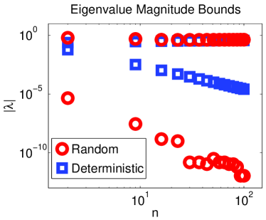
Figure 1: Red circles are the magnitude of upper and lower bounds for eigenvalues of $A_{\mathbb{X}_{(n)}(P)}^{-1}$. For each $n$, $m=12000$ random grids were sampled from a uniform distribution and eigenvalues of the corresponding $A_{\mathbb{X}_{(n)}(P)}^{-1}$ were computed. For comparison, the blue squares are the magnitudes of the upper and lower bounds for the eigenvalues of $A_{Q^{0}(\mathbf{x}_{n}^{0})}^{-1}$.

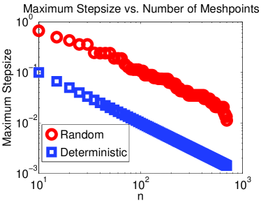
Figure 2: Red circles illustrate the convergence of the largest step-size in randomly generated meshes of length $n$. For each $n$, $m=1000$ meshes $\mathbb{X}_{(n)}(P)$ were generated for $P$ a uniform distribution on $\bar{\mathbf{I}}$. The vertical axis is the maximum step-size between and two nearby points in $\mathbb{X}_{(n)}(P)$. For comparison, we also include the step-sizes for a uniform partition of the domain (blue squares).

Theorem 5.

Under Condition C1 and C2, the expected error converges pointwise to zero.

Proof.

Let $e_{k}$ be a vector of zeros with a one in the $k$th element and $\mathbb{X}_{(n),\xi,k}$ denote the vector $(X_{(1)},\ldots,X_{(k-1)},\xi,X_{(k+1)},\ldots,X_{(n)})$ where the $k$th element of $\mathbb{X}_{(n)}$ is replaced by $\xi$. Consider the pointwise error between the the analytical solution $u$ and mean of the coarse-mesh solutions $\mu$

$$\left\|u(\xi)-\mu(\xi;U(\mathbb{X}_{(n)}(P)))\right\| = \left\|u(\xi)-\mathbb{E}_{P}\left[\mathbb{E}_{K}\left[\{U(\mathbb{X}_{(n)}(P))\}_{K}\left|K:X_{(K)}=\xi\right.\right]\right]\right\|$$

$$= \left\|\mathbb{E}_{P}\left[\mathbb{E}_{K}\left[u(\xi)-\{U(\mathbb{X}_{(n)}(P))\}_{K}\left|K:X_{(K)}=\xi\right.\right]\right]\right\|$$

$$= \left\|\mathbb{E}_{P}\left[\mathbb{E}_{K}\left[u(\xi)-e_{K}^{T}(U(\mathbb{X}_{(n)}(P))\left|K:X_{(K)}=\xi\right.\right]\right]\right\|$$

$$\leq \mathbb{E}_{P}\left[\mathbb{E}_{K}\left[\left\|e_{K}^{T}(u(\mathbb{X}_{(n),\xi,K})-U(\mathbb{X}_{(n)}(P))\right\|\left|K:X_{(K)}=\xi\right.\right]\right]$$

$$\leq \mathbb{E}_{P}\left[\left\|A_{\mathbb{X}_{(n)}(P)}^{-1}\right\|\cdot\mathbb{E}_{K}\left[\left\|A_{\mathbb{X}_{(n)}(P)}u(\mathbb{X}_{(n),\xi,K})-f_{\mathbb{X}_{(n)}}\right\|\left|K:X_{(K)}=\xi\right.\right]\right]\,.$$

We note that $\left\|A_{\mathbb{X}_{(n)}(P)}u(\mathbb{X}_{(n),\xi,k})-f_{\mathbb{X}_{(n)}}\right\|$ is the truncation error induced from a 3-point non-uniform centered-difference stencil and converge as $\mathcal{O}(\max_{i=1,\ldots,n-1}|X_{(i)}-X_{(i+1)}|)$ (Figure 2 also depicts this behavior). Therefore, assuming Conditions C1 and C2, we can conclude that the error converges pointwise. ∎

2.4 Criteria Motivation

In Section 3, we consider problems containing second derivatives as well as nonlinear functions of first derivatives. We create $Q$ depending upon the specific problem class under consideration. In one case, $Q$ is based upon the derivative of the mean of the solutions $\mu$, while in another we consider the product of the variance and the the second derivative of $\mu$. In all cases, however, $Q$ is created using the statistical moments of the sampled sparse-mesh solutions and the results suggest that a more generalizable strategy may exist.

For the problems with second derivatives (equation (3.1) in Subsection 3.1 and equation (14) in Subsection 3.3) we define $Q$ as

$$Q(x)=\left[\frac{q_{1}(\cdot)}{q_{1}(1)}\right]^{-1}(x)\,,$$

where

$$q_{1}(x)=\int_{0}^{x}\sqrt{\left|\mu^{\prime}(\xi;U(\mathbb{X}_{(n)}(P))\right|}d\xi\,,$$

and the superscript $-1$ is an inverse function operator. Essentially, this definition will pile up points in regions with a steep solution in an effort to provide higher order accuracy for the nonuniform second derivative discretization.

For the problem with a third power of the first derivative (equation (10) in Subsection 3.2), we define $Q$ as

$$Q(x)=\left[\frac{q_{2}(\cdot)}{q_{2}(1)}\right]^{-1}(x)\,,$$

where

$$q_{2}(x)=\int_{0}^{x}\mu^{\prime\prime}(\xi;U(\mathbb{X}_{(n)}(P))^{2}\,v(\xi;U(\mathbb{X}_{(n)}(P))^{3}d\xi\,,$$

and $v$ is from Definition (4).

To motivate these mappings, consider a least squares cost function $J:\mathbb{R}\to\mathbb{R}$ which compares (pointwise) a proposed solution to the actual solution $u$ at an arbitrary point $\xi\in\bar{\mathbf{I}}$. We then consider the random variable $J(\mu(\xi,\mathbb{X}_{(n)}(P))$ and Taylor series expand the expected value of $J$ around a local minimum $\mu^{*}(\xi)$ for some $\xi\in\mathbf{I}$

$$\mathbb{E}_{P}\left[J(\mu(\xi,\mathbb{X}_{(n)}(P))\right]\approx\mathbb{E}_{P}\left[J(\mu^{*}(\xi))+J_{1}+J_{2}\right]$$

where

$$J_{1} = J^{\prime}(\mu^{*}(\xi))(\mu(\xi,\mathbb{X}_{(n)}(P))-\bar{\mu}^{*}(\xi))$$

and

$$J_{2} = J^{\prime\prime}(\mu^{*}(\xi))\left(\mu(\xi,\mathbb{X}_{(n)}(P))-\mu^{*}(\xi)\right)^{2}\,.$$

Note that since $\mu^{*}$ is assumed to be a local minimum for $J$ , $J_{1}\equiv 0$ and that in $J_{2}$, $J^{\prime\prime}(\mu^{*}(\xi))=1$. The expected cost function can thus be approximated by

$$\begin{array}[]{l}\mathbb{E}_{P}\left[J(\mu(\xi,\mathbb{X}_{(n)}(P)))\right]\approx\mathbb{E}_{P}\left[J(\mu^{*}(\xi))\right]+\mathbb{E}_{P}\left[\left(\mu(\xi,\mathbb{X}_{(n)}(P))-\mu^{*}(\xi)\right)^{2}\right]\,.\end{array}$$ (7)

According to Theorem 5, $\lim_{n\to\infty}\mathbb{E}_{P}\left[J(\mu^{*}(\xi))\right]=0$ pointwise. Most importantly, the second term in (7) is the variance of $\mu(\xi,\mathbb{X}_{(n)}(P))$. The moments of the sparse sampled solutions, therefore, can offer insight into the actual solution.

We hypothesize that the reason $q_{1}(x)$ works well is that the $\mu^{\prime}$ may converge faster than $\mu$. A full investigation will require establishing the appropriate Sobolev space, though it is not immediately clear how to proceed.

We also hypothesize that the function $q_{2}(x)$ works well because the second derivative (when cast as the local curvature) is inversely proportional to the local variance of a random variable (a result which is well known in the semi-parametric nonlinear regression literature [23]). Essentially, while the $\mu^{\prime\prime}$ may not converge quickly, the product $\mu^{\prime\prime}v$ does. We also found that multiplication by an extra $v$ dramatically improves the computed $Q$, though an explanation is not immediately clear. A deeper understanding of the spectrum of $A_{\mathbb{X}_{(n)}(P)}$ and how it depends upon the choice of $P$ will be essential to explaining the efficiency of $q_{2}(x)$. We plan to explore both of these issues in a future paper.

2.5 Sampling Strategy

The proposed methodology relies on random sampling and sorting a sampled vector from a distribution. For standard sampling problems, the confidence intervals for variance estimation converge as $\mathcal{O}(\sqrt{m})$ for $m$ samples. In the absence of a full theoretical analysis, we offer numerical evidence supporting our accurate computation of the variance. Note that in all the following simulations, we use the first example problem presented in Section 3, the singular two-point BVP (8)-(9).

The relationship between the mesh size $n$ and the number of samples $m$ is non-trivial. and Figure 3 illustrates this by depicting the error in $\bar{v}$ (relative to $\bar{v}$ computed with $m=3000$ sampled from a uniform distribution on $\bar{\mathbf{I}}$) for a range of $n$ and $m$ values. For a given $n$, though, we do note that the error in the $\bar{v}$ computation is decreasing. In Figure 4 we depict the number of samples of vector size $n$ which are needed to ensure three digits of accuracy in estimating the variance. Since the number was consistently below $1000$ over a range of $n$, we let $m=15000$ in all subsequent simulations (unless otherwise specified).

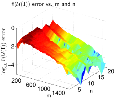
Figure 3: $\log_{10}$ of the error in the computation of $\bar{v}$ (sampling from a uniform distribution on $\bar{\mathbf{I}}$) as a function of $m$ and $n$. Note the general downward trend along both the $m$ and $n$ axes.

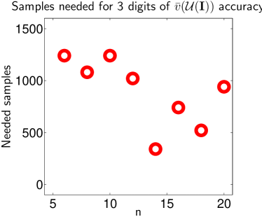
Figure 4: For each $n,$ the vertical axis reflects the number of samples needed to compute the variance with 3 digits of accuracy relative to $\bar{v}$ (sampling from uniform distribution on $\bar{\mathbf{I}}$) with $m=3000$.

We also note that figures with similar conclusions can be generated for the other problems described in Section 3.

3 Numerical Simulations

In this section, we consider three classes of BVP’s and illustrate the effectiveness of our approach in identifying a non-uniform mesh spacing which yields a solution accuracy superior to that of uniform spacing. The examples in Sections 3.1-3.2 were chosen because the solutions exhibited changes in smoothness such as boundary layers and a discontinuity in the derivative, i.e., a local effect. The example in Section 3.3 was chosen because the solutions exhibited varying multi-scale oscillations over the domain, i.e., a global effect.

All software development was done in Matlab and in particular, parallel for-loops (parfor) were used whenever possible. For all simulations, we let $m=15000$ unless otherwise specified. A copy of the software is available upon request to the corresponding author.

3.1 Singular Boundary Value Problem

The following singular two-point Boundary Value Problem

$$(x^{\alpha}u^{\prime})^{\prime}=f(x,u) ;\,0\leq x\leq 1$$ (8)

$$u(0)=A ;\,u(1)=B$$ (9)

encompasses a large class of singular BVP’s where $\alpha\in(0,1)$ and $A$, $B$ are finite and constant. For $(x,y)\in\{[0,1]\times\mathbb{R}\}$ such that $f(x,y)$ is continuous, $\partial f/\partial x$ exists and is continuous and $\partial f/\partial y\geq 0$. Many researchers have successfully implemented strategies to solve classes of singular BVP’s using uniform finite difference [13], Rayleigh-Ritz-Galerkin [9], projection [21], and collocation [22] schemes.

We consider the specific problem presented in [3] for $f(x,u)=\beta x^{\alpha+\beta-2}((\alpha+\beta-1)+\beta x^{\beta})u$, $A=1$, $B=e$ and with exact solution $u(x)=\exp(x^{\beta})$. Depicted in Figure (5) is the solution for $\alpha=.85$, and $\beta=10$; note the strong boundary layer affect near $x=1$.

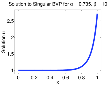
Figure 5: Analytical solution to singular two-point Boundary Value Problem in (8)-(9) for $f(x,u)=\beta x^{\alpha+\beta-2}((\alpha+\beta-1)+\beta x^{\beta})u$, $u(0)=1$, and $u(1)=e$.

Inspired by the fact that a non-uniform mesh provides superior accuracy for this class of problems (as investigated in [3, 5]), we consider the mapping $Q_{\alpha}(x)=x^{1-\alpha}$. We choose $\alpha=0.735$, $Q_{0.735}(x)=x^{1-0.735}$ because for $n=100$, this $Q_{0.735}$ yields 2.4 orders of magnitude more accuracy in the solution than $Q^{0}$. The dotted curve in Figure 7 depicts the corresponding plot of $Q_{0.735}$ and should thus be considered a gold standard, with which we will compare our computed mapping.

For this problem, we first consider $m=15000$ samples of length $n=10$ and solve (8)-(9). Figure 6 depicts a contour plot of the probability density of $p(\xi;\mathbb{X}_{(n)}(P))$, where $P$ is a uniform distribution on $\bar{\mathbf{I}}$. We note that many of the sparse solutions have relatively large values for $x$ near $3/4$, but we are at a loss to explain this phenomenon. Figure 7 depicts our computed $Q$ along with the uniform and analytically optimal mappings and Figure 8 depicts the error convergence properties for $Q$ and $Q^{0}$. We draw attention to the fact that for mesh sizes less than $100$, our mapping results in second order convergence, even though the discretization is first order. Indeed, the error is at times, marginally better than $Q_{\alpha}$. We also note that while $Q^{0}$ and $Q_{\alpha}$ are second order accurate, our non-uniform mapping asymptotically converges with first-order accuracy. Lastly, Figure 9a depicts solutions using $n=20$ mesh-points from the uniform and computed optimal mappings. The uniform mesh creates a solution which is consistently above the analytical solution, while the solution computed from $Q$ is substantially more accurate for small numbers of mesh points. While the difference between the solution is visually small, it is almost an order of magnitude more accurate and Figure 9b depicts the solution residuals.

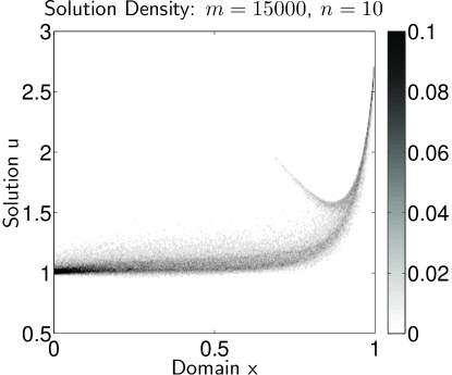
Figure 6: Contour plot of the probability density of $p(x,\mathbb{X}_{(n)}(P))$ for $m=15000$ sampled meshes of length $n=10$ from mesh mapping $Q^{0}$ and $P$ a uniform distribution on $\bar{\mathbf{I}}$.

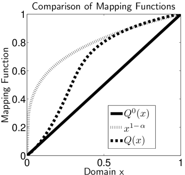
Figure 7: Comparison of different mesh mappings. The solid line is uniform spacing $Q^{0}(x)$, the dotted line is the analytically optimal non-uniform spacing $x^{(1-\alpha)}$, and dot-dashed line with the circles is the computed $Q(x)$.

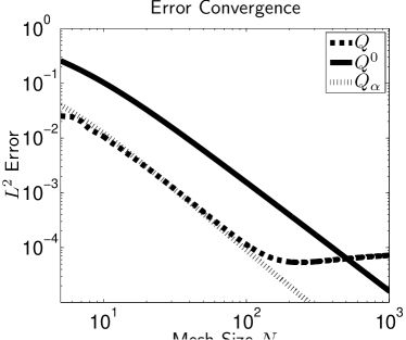
Figure 8: Error convergence of the different mesh mappings.

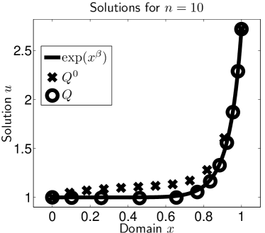
a) b)

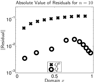
Figure 9: a) Solution using $n=10$ mesh points. The solid line is the analytical solution. The ’X’ and ’O’ symbols are the solutions generated using the uniform ($Q^{0}$) and computed ($Q$) mesh point mappings. b) The absolute value of the pointwise residuals for both solutions.

3.2 Hamilton-Jacobi Equation

An important example problem which may develop a singularity at an internal location is the time-invariant Hamilton-Jacobi (HJ) equation,

$$u+H(u_{x})=f ;\,0\leq x\leq 1,$$ (10)

$$u(0) = u(1)$$ (11)

where we assume period Dirichlet boundary conditions. We consider

$$H(p)=\frac{p^{2}}{\pi^{2}}\;,\;\;f(x)=-\left|\sin(\pi(x-\frac{\pi}{4}))\right|+\cos^{2}(\pi(x-\frac{\pi}{4}))\,,$$ (12)

which yields a solution $u(x)=-|\sin\left(\pi\left(x-\frac{\pi}{4}\right)\right)|$ with a discontinuity in the derivative at $\frac{\pi}{4}$. The analytical solution on $\bar{\mathbf{I}}$ is depicted in Figure 10.

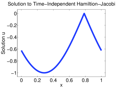
Figure 10: Analytical solution to time-independent Hamilton-Jacobi equation in (10)-(11) for $H(p)=\frac{p^{2}}{\pi^{2}}$ and $f(x)=-\left|\sin(\pi(x-\frac{\pi}{4}))\right|+\cos^{2}(\pi(x-\frac{\pi}{4}))$.

For this problem, we first consider $m=15000$ samples of length $n=10$ and solve (10)-(12). We discretized $u_{x}$ using centered differences and then solved this nonlinear PDE by minimizing the norm of the residual ($u+H(u_{x})-f$) using a Quasi-Newton method with BFGS update. Figure 11 depicts the contour plot of the probability density of $p(\xi;\mathbb{X}_{(n)}(P))$ where $P$ is a uniform distribution on $\mathbf{I}$.

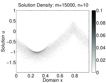
Figure 11: Contour plot of the probability density of $p(x,\mathbb{X}_{(n)}(P))$ for $m=15000$ sampled meshes of length $n=10$ for Hamilton-Jacobi problem in (10)-(12), where $P$ is a uniform distribution on $\bar{\mathbf{I}}$.

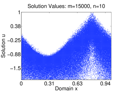
Figure 12: Point cloud of solution values for $m=15000$ sampled meshes of length $n=10$ for Hamilton-Jacobi problem in (10)-(12).

Figure 13 depicts our computed optimal $Q$ along with the uniform and analytically optimal mappings while Figure 14 depicts the convergence properties for the different mappings. We note that computed mapping will result in many mesh-points near $\pi/4$, which is exactly the location of the derivative discontinuity in the solution. Figure 14 depicts the convergence in error for uniformly and non-uniformly spaced points as specified by the mappings defined in Figure 13. We note that our strategy offers a substantial improvement in solution accuracy for small numbers of mesh-points; it even overcomes the inherent instability of centered-differences. To illustrate the improved accuracy for small $n$, Figure 15 depicts a) the solutions generated by $Q$ and $Q^{0}$ as well as b the absolute value of the pointwise residuals for both mesh-point mappings.

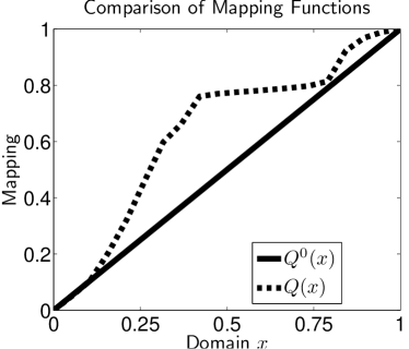
Figure 13: Mapping functions $Q$ and $Q^{0}$. Note how there will be a large percentage of the points at $\pi/4$.

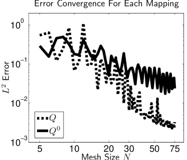
Figure 14: Error convergence for uniformly and non-uniformly spaced points where the non-uniform spacing is determined by the mapping in Figure 13.

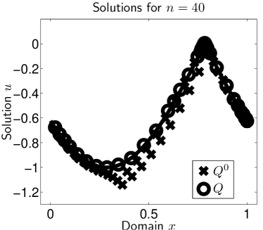
a) b)

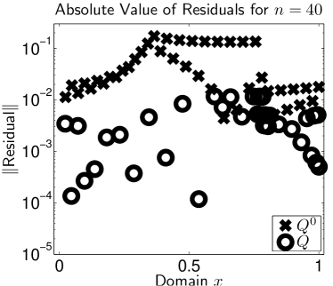
Figure 15: a) Solution to the HJ equation (10)-(13) with $n=40$ mesh-points using the computed non-uniform mapping circles ’O’ and uniformly spaced mesh-point ’X’. b) The absolute value of the pointwise residuals for both solutions.

3.3 Oscillatory Boundary Value Problems

The following problem was selected from [18] specifically because it illustrates a situation for which our approach does not perform well. Consider the specific Poisson problem

$$u^{\prime\prime}(x) = -20+\frac{1}{2}\phi^{\prime\prime}(x)\cos(\phi(x))-\frac{1}{2}(\phi^{\prime}(x))^{2}\sin(\phi(x))$$ (14)

$$u(0)=1\,;\,u(1)=3$$

with $a=0.5$. The solution with Dirichlet boundary conditions $u(0)=1$, $u(1)=3$ is

$$u(x)=1+12x-10x^{2}+a\sin(\phi(x))\,.$$

This analytical solution is depicted for $\phi(x)=5\pi x^{3}$ and $\phi(x)=20\pi x^{3}$ in Figures 16a and 16b, respectively.

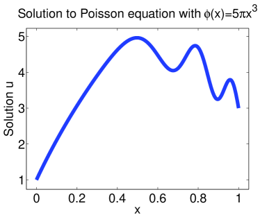
a) b)

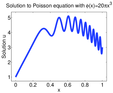
Figure 16: Analytical solution to Poisson equation from with a) $\phi(x)=5\pi x^{3}$ and b) $\phi(x)=20\pi x^{3}$ from [18].

As with the other problems, we first consider $m=15000$ samples of length $n=10$ and solve (14)-(14). Figure 17 depicts contour plots of the probability density of $p(\xi;\mathbb{X}_{(n)}(P))$, where $P$ is a uniform distribution on $\bar{\mathbf{I}}$, for $\phi(x)=5\pi x^{3}$ and $\phi(x)=20\pi x^{3}$ in Figures 17a and 17b, respectively. We note the relatively large total variance and that higher frequency forcing oscillations appear to correlate with larger variance and plan to investigate this in a future article.

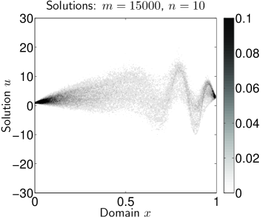
a) b)

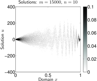
Figure 17: Contour plot of the probability density of $p(x,\mathbb{X}_{(n)}(P))$ for $m=15000$ sampled meshes of length $n=10$ for the Poisson equation defined in (14)-(14), where $P$ is a uniform distribution on $\bar{\mathbf{I}}$.

Figures 18a) and 18b depict our computed $Q$ for the two $\phi(x)$ functions along with the uniform mapping using $n=10$. Figure 19 depicts the convergence in error for uniformly and non-uniformly spaced points as specified by the mappings defined in Figure 18. Here, the $Q$ computed by our approach is noticeably worse than using a uniform spacing.

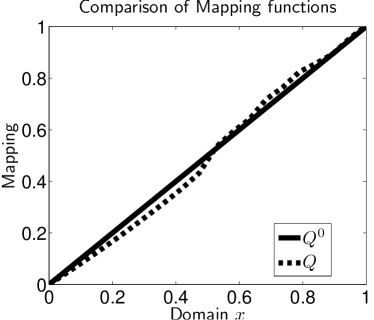
a) b)

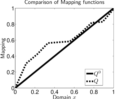
Figure 18: Mapping functions $Q$ and $Q^{0}$ for a) $\phi(x)=5\pi x^{3}$ and b) $\phi(x)=20\pi x^{3}$.

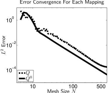
a) b)

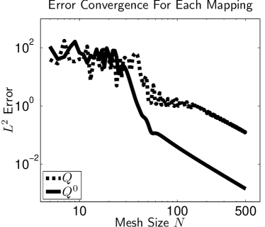
Figure 19: Error convergence for uniformly and non-uniformly spaced points where the non-uniform spacing is determined by the mapping in Figure 18.

4 Summary

4.1 Conclusions and Future Work

In this article, we have proposed a strategy for identifying non-uniform mappings to improve solution accuracy when using a smaller number of points. We find that our strategy performs well when faced with local phenomena, i.e., when there is a subset of the domain which would benefit from a higher density of mesh-points. With behaviors which are fundamentally global, such as oscillations, our approach fares no better than with uniformly placed points.

The immediate goal for the next article is to apply our approach to higher dimensional systems where we envision the benefit of the $\mathcal{O}(\sqrt{m})$ convergence (independent of $n$) will become even more pronounced. With the recent release of software to enable calling CUDA (Compute Unified Device Architecture [10]) from Matlab, we also plan to develop an implementation on a GPGPU. Among the open theoretical questions we plan to investigate in followup articles, the most pressing is how to formalize taking the information in the point cloud of sparse-mesh solutions and construct $Q$. We envision development of a criteria, which is based in part on the operator discretization strategy and part on the form of the PDE.

Our algorithm could also greatly benefit from connections to the experimental design literature. There are criteria designed to aid in choosing optimal sampling locations, which could provide a more efficient computation of $Q$ [1]. Our original vision for this work involved casting $P^{-1}$ as the mapping $Q$ and developing an inverse problem strategy to identify an optimal $P^{*}$ via optimizing $\bar{v}(P)$. For this paper, the optimization was not nearly as efficient as simply computing $Q$. There are, however, stochastic approximation algorithms (such as Kiefer-Wolfowitz [16]) which are designed to optimize stochastic functions and there is significant literature within the control theory community on this topic [17]. This would allow reduction in the number of samples needed to compute the total variance. We also plan to investigate an improved strategy for the function approximation choices (such as how many $n$ are needed). A long-term goal is to investigate how our approach could be used to update a given set of mesh-points to improve accuracy. Lastly, there are many opportunities to extend the theoretical analysis. In particular, the function theoretic basis for the finite element approach could prove useful in establishing convergence the the appropriate Sobolev space. Lastly, the rich literature of random matrix theory will of course improve our knowledge of the distribution of eigenvalues for the approximate finite difference operator.

4.2 Discussion

The widespread availability of massively multi-core architectures such as General-Purpose Graphics Processing Units (GPGPU’s) provides a unique opportunity for investigating non-traditional and non-conventional approaches to solving computational problems. It is an opportunity to completely re-imagine traditional numerical analysis algorithms. For example, in [8], the authors propose a parallel ODE solver which would be particularly slow on single-core CPU’s. However, when implemented on a GPGPU, it can realize spectacular improvements in computational efficiency and accuracy. Similarly, the approach presented above rests on the notion that future trends in architecture design will produce processors with a large numbers of computational cores and relatively modest memory resources. Accordingly, we envision that the implementation of the sampling step on a GPGPU will yield substantial speedups in efficient mesh generation, since the algorithm will theoretically scale with the number of computational cores. Like the parallel ODE solver in [8], a single-core implementation would be completely unacceptable. We assert that algorithms in this class are beyond embarrassingly parallel; implementing it on anything but a massively multi-core architecture would be scandalous.

5 Acknowledgments

D. M. Bortz and A. J. Christlieb are supported in part by DOD-AFOSR grant FA9550-09-1-0403. The authors would also like to thank V. Dukić for insightful comments on an earlier draft of this manuscript.

Appendix A Notation

• Matrix generated by a three point stencil (potentially non-uniform) discretizing the second derivative in a Poisson equation. The subscript indicates the set of points to use in the discretization.

• Vector generated by evaluating the forcing function in a Poisson equation. The subscript indicates the set of points to use in the discretization.

• Domain for the BVP. In this work, $\mathbf{I}=(0,1)$ and $\bar{\mathbf{I}}=[0,1]$. It is also the probability sample space for $X$.

• Number of sampled meshes.

• Pointwise mean of $p$, which allows computation of the expected value of the approximate solutions at a given point $\xi\in\mathbf{I}$, given that $\xi$ is a point in the mesh.

• Number of points in a given mesh.

• Function mapping a random vector of length $n$ and a point $\xi\in\mathbf{I}$ to a random variable.

• Probability distribution.

• Mesh function which maps $\mathbf{I}\to\mathbf{I}$.

• Taylor Series truncation error from using a three point stencil to discretize the second derivative on a (potentially non-uniform) mesh. The subscript indicates the set of point to use in the discretization.

• Analytical solution to a BVP.

• $n$-dimensional numerical approximation to $u$.

• Function which maps $\mathbf{I}^{n}\to\mathbb{R}^{n}$ taking a mesh and solving a given BVP on those mesh points.

• Pointwise variance of $p$, which allows computation of the variance of the approximate solutions at a given point $\xi\in\mathbf{I}$, given that $\xi$ is a point in the mesh.

• Average of variance $v$ over $\bar{\mathbf{I}}$.

• Mesh of $n$ uniformly spaced points in $\mathbf{I}$.

• Random variable with distribution $P$.

• Vector of $n$ i.i.d. random variables. $\mathbb{X}_{n}=(X_{1},X_{2},\ldots,X_{n})^{T}$.

• Sorted vector of $n$ i.i.d. random variables. $\mathbb{X}_{(n)}=(X_{(1)},X_{(2)},\ldots,X_{(n)})^{T}$.

• Arbitrary point in $\mathbf{I}$.

References

- [1] A. C. Atkinson and A. N. Donev. Optimal Experimental Design, volume 8 of Oxford Statistical Science Series. Oxford University Press, 1992.
- [2] K. Atkinson. An Introduction to Numerical Analysis. Wiley, New York, NY, 2nd edition, 1989.
- [3] T. Aziz and M. Kumar. A fourth-order finite-difference method based on non-uniform mesh for a class of singular two-point boundary value problems. J. Computational & Applied Math., 136:337–342, 2001.
- [4] R. E. Caflisch. Monte Carlo and quasi-Monte Carlo methods. Acta Numerica, 7:1–49, 1998.
- [5] M. M. Chawla and C. P. Katti. Finite difference methods and their convergence for a class of singular two point boundary value problems. Numerische Mathematik, 39:341–350, 1982.
- [6] C. S. Chen, M. A. Golberg, and Y. C. Hon. The method of fundamental solutions and quasi-Monte Carlo method for diffusion equations. Int. J. for Numerical Methods in Eng., 43:1421–1435, 1998.
- [7] W. Chen and J. He. A study on radial basis function and quasi-Monte Carlo methods. Int. J. Nonlinear Sciences & Numerical Simulation, 1(4):343–342, 2000.
- [8] A. J. Christlieb and B. Ong. Implicit parallel time integrators. J. Scientific Computing, 2011. To appear.
- [9] P. G. Ciarlet, F. Natterer, and R. S. Varga. Numerical methods of high order accuracy for singular nonlinear boundary value problems. Numerische Mathematik, 15:87–99, 1970.
- [10] CUDA: Compute Unified Device Architecture. http://www.nvidia.com.
- [11] H. A. David and H. N. Nagaraja. Order Statistics. Wiley Series in Statistics. Wiley, New York, NY, 2003.
- [12] I. Friedel and A. Keller. Fast generation of randomized low-discrepancy point sets. In H. Niederreiter, K. Fang, and F. Hickernell, editors, Monte Carlo and Quasi-Monte Carlo Methods 2000, pages 257–273. Springer-Verlag, 2001.
- [13] P. Jamet. On the convergence of finite difference approximations to one-dimensional singular boundary value problems. Numerische Mathematik, 14:355–378, 1970.
- [14] S. Karni and A. Kurganov. Local error analysis for approximate solutions of hyperbolic conservation laws. Adv. Computational Math., 22:79–99, 2005.
- [15] S. Karni, A. Kurganov, and G. Petrova. A smoothness indicator for adaptive algorithms for hyperbolic systems. J. Computational Physics, 178:323–341, 2002.
- [16] J. Kiefer and J. Wolfowitz. Stochastic estimation of the maximum of a regression function. Ann. Math. Statistics, 23(3):462–466, Sep. 1952.
- [17] H. J. Kushner and G. G. Yin. Stochastic Approximation and Recursive Algorithms and Applications, volume 35 of Applications of Mathematics. Springer-Verlag, New York, NY, 2nd edition, 2003.
- [18] R. J. LeVeque. Finite Difference Methods for Ordinary and Partial Differential Equations: Steady-State and Time-Dependent Problems. SIAM, Philadelphia, PA, 2007.
- [19] W. J. Moroko and R. E. Caflisch. Quasi-Monte Carlo integration. J. Computational Physics, 122:218–230, 1995.
- [20] H. Niederreiter. Quasi-Monte Carlo methods and pseudo-random numbers. Bull. Am. Math. Soc., 84:957–1041, 1978.
- [21] G. W. Reddien. Projection methods and singular two-point boundary value problems. Numerische Mathematik, 21:193–205, 1973.
- [22] G. W. Reddien and L. L. Schumaker. On a collocation method for singular two-point boundary value problems. Numerische Mathematik, 25:427–432, 1976.
- [23] G. A. F. Seber and C. J. Wild. Nonlinear Regression. John Wiley & Sons, New York, NY, 1989.