Enhancement of Diffusive Transport by Nonequilibrium Thermal Fluctuations

Abstract

We study the contribution of advection by thermal velocity fluctuations to the effective diffusion coefficient in a mixture of two indistinguishable fluids. The steady-state diffusive flux in a finite system subject to a concentration gradient is enhanced because of long-range correlations between concentration fluctuations and fluctuations of the velocity parallel to the concentration gradient. The enhancement of the diffusive transport depends on the system size $L$ and grows as $\ln(L/L_{0})$ in quasi-two dimensional systems, while in three dimensions it grows as $L_{0}^{-1}-L^{-1}$, where $L_{0}$ is a reference length. The predictions of a simple fluctuating hydrodynamics theory, closely related to second-order mode-mode coupling analysis, are compared to results from particle simulations and a finite-volume solver and excellent agreement is observed. We elucidate the direct connection to the long-time tail of the velocity autocorrelation function in finite systems, as well as finite-size corrections employed in molecular dynamics calculations. Our results conclusively demonstrate that the nonlinear advective terms need to be retained in the equations of fluctuating hydrodynamics when modeling transport in small-scale finite systems.

I Introduction

Thermal fluctuations in non-equilibrium systems in which a constant (temperature, concentration, velocity) gradient is imposed externally exhibit remarkable behavior compared to equilibrium systems. Most notably, external gradients can lead to enhancement of thermal fluctuations and to long-range correlations between fluctuations DSMC_Fluctuations_Shear ; Mareschal:92 ; LongRangeCorrelations_MD ; Zarate:04 ; FluctHydroNonEq_Book . This phenomenon can be illustrated by considering concentration fluctuations in an isothermal mixture of two miscible fluids, subjected to a macroscopic concentration gradient $\boldsymbol{\nabla}c$. The solution of the linearized equations of fluctuating hydrodynamics shows that concentration and density fluctuations exhibit long-range correlations, leading to a power-law divergence of the static structure factors for small wavenumbers $k$. When the species have different molecular masses and gravity $\boldsymbol{g}$ is present, the analysis predicts that fluctuations at wavenumbers below $k_{g}\sim\left(\boldsymbol{g}\cdot\boldsymbol{\nabla}c\right)^{1/4}$ are suppressed GiantFluctuations_Nature ; GiantFluctuations_Theory ; GiantFluctuations_Universal ; GiantFluctuations_Microgravity ; GiantFluctuations_Cannell ; FractalDiffusion_Microgravity , where $c$ is the mass concentration of the heavier species. Similar conclusions hold for fluctuations in a single-component fluid subject to a stabilizing temperature gradient TemperatureGradient_Cannell .

It is important to emphasize that this enhancement of large-scale (small wavenumber) concentration fluctuations occurs because of the non-equilibrium setting, and not because of the concentration gradient itself. Specifically, the enhancement is related to the dissipative flux through the system LLNS_Schmitz , which is zero at thermodynamic equilibrium. The top left panel of Fig. 1 shows a snapshot of the concentration field for a two-dimensional system in thermodynamic equilibrium in which there is a concentration gradient because of the sedimentation of the heavier species due to gravity, but no enhancement of the fluctuations. By comparison, the top right panel of the figure shows a non-equilibrium system with similar parameters but with an externally-imposed concentration gradient (via the top and bottom wall boundary conditions) and no gravity, revealing much-enhanced fluctuations (noise) and large-scale features (clumping). If gravity is included in addition to the external gradient, the total diffusive flux is reduced and large-scale fluctuations (wavenumber $k\lesssim k_{g}$) are suppressed, as shown in the bottom left panel of Fig. 1. In fact, if the same gravity as in the equilibrium case is imposed in addition to the external gradient, the total diffusive flux is essentially zero and the system is close to equilibrium again, giving no visible enhancement of the concentration fluctuations over the equilibrium case, as shown in the bottom right panel of Fig. 1. These illustrative numerical results were obtained using a finite-volume solver for compressible fluctuating hydrodynamics LLNS_S_k .

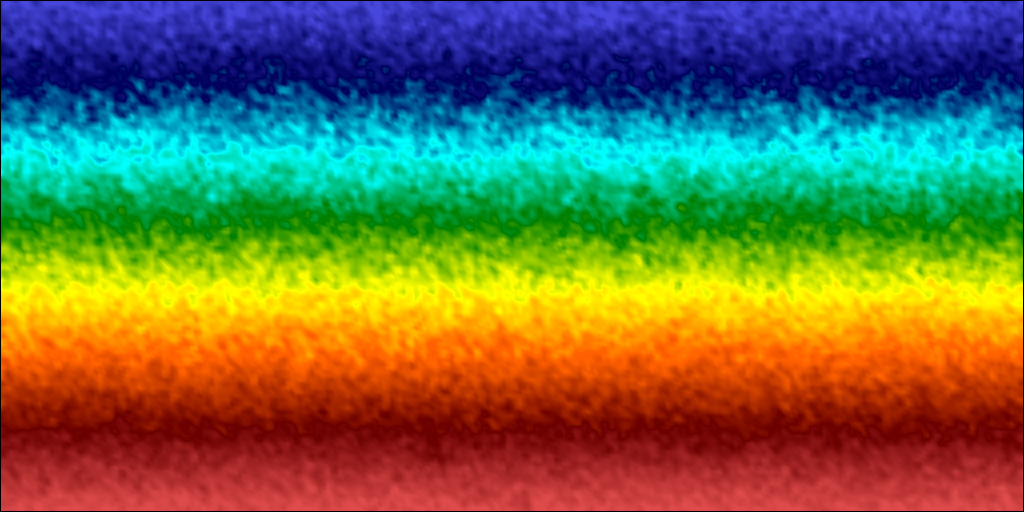
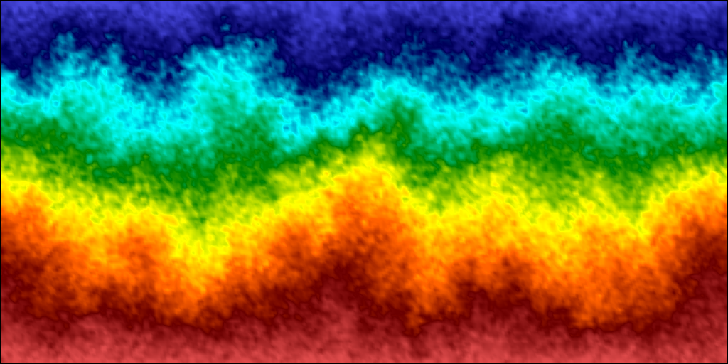
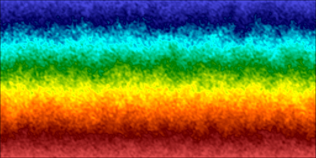
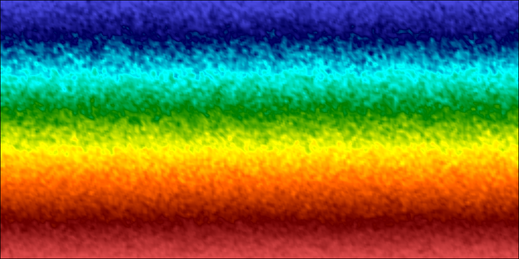
Figure 1: Snapshot of the local concentration for a mixture of two ideal gases in a quasi-two-dimensional system, as obtained from a long run of a compressible finite-volume solver which includes thermal fluctuations LLNS_S_k , with constant-temperature walls placed at the top and bottom boundary. The particles of species 1 (red end of the color scale) are four times heavier than particles of species 2 (blue end of the color scale), and all systems are in mechanical equilibrium (i.e., the gravity force is balanced by the pressure gradient). (Top left panel) A system at equilibrium, in the presence of gravity $g_{0}$, with the heavier particles sedimenting toward the bottom according to the equilibrium Gibbs-Boltzmann distribution. (Top right panel) No gravity but a similar non-equilibrium concentration profile as in the top left panel is imposed via Dirichlet boundary conditions at the top and bottom walls, showing giant concentration fluctuations. (Bottom left panel) The same boundary conditions for the concentration are imposed as in the top right panel, but with gravity $g=0.1\,g_{0}$, showing a suppression of the large-scale giant fluctuations. (Bottom right panel) The same boundary conditions for the concentration are imposed as in the top right panel, but with the same gravity $g=g_{0}$ as in the top left panel, showing no enhancement of the fluctuations.

The enhancement of concentration fluctuations is even more dramatic if the concentration gradient is at an interface, as in the study of the early stages of diffusive mixing between initially separated fluid components. As illustrated in Fig. 2, the interface between the fluids, instead of remaining flat, develops large-scale roughness that reaches a pronounced maximum until gravity or boundary effects intervene. These giant fluctuations GiantFluctuations_Theory ; TemperatureGradient_Cannell ; GiantFluctuations_ThinFilms during free diffusive mixing have been observed using light scattering and shadowgraphy techniques GiantFluctuations_Nature ; GiantFluctuations_Universal ; GiantFluctuations_Microgravity ; GiantFluctuations_Cannell ; FractalDiffusion_Microgravity , finding good but imperfect agreement between the predictions of a simplified fluctuating hydrodynamic theory and experiments. In the absence of gravity, the density mismatch between the two fluids does not change the qualitative nature of the non-equilibrium fluctuations, and in this work we focus on the case of two dynamically-indistinguishable fluids.

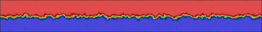
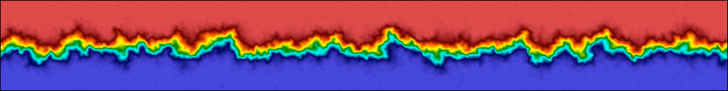
Figure 2: The rough diffusive interface between two miscible fluids at three points in time (top to bottom), starting from an initially perfectly flat interface (phase separated system), without gravity. Compare to the top right panel in Fig. 1.

The giant fluctuation phenomenon arises because of the appearance of long-range correlations between concentration and velocity fluctuations in the presence of a concentration gradient. Based on nonlinear fluctuating hydrodynamic theory, it has been predicted that these correlations give rise to fluctuation-renormalized transport coefficients at larger scales DiffusionRenormalization_I ; DiffusionRenormalization_II ; ExtraDiffusion_Vailati . However, the predicted contribution from fluctuations to transport at mesoscopic and macroscopic scales has only recently been computationally observed and reported by the authors DiffusionRenormalization_PRL . This paper presents a detailed exposition of both the theoretical prediction for the enhancement of diffusion and the numerical simulations verifying these predictions. In particular, it is important to understand how the effective transport coefficients depend on the length scale of observation. This length scale may be related to the length $\Delta x$ of the finite-volume cells used in a fluctuating hydrodynamic solver, or it may be related to the physical dimensions of a finite system such as a nano-channel transporting liquid or a nano-wire transporting heat.

We consider diffusion in a mixture of dynamically identical but labeled (as components 1 and 2) fluids SelfDiffusion_Linearity enclosed in a box of lengths $L_{x}\times L_{y}\times L_{z}$, in the absence of gravity. Periodic boundary conditions are applied in the $x$ (horizontal) and $z$ (depth) directions, and impermeable constant-temperature walls are placed at the top and bottom boundaries. A concentration gradient $\nabla\bar{c}=(c_{T}-c_{B})/L_{y}$ is imposed along the $y$ axes by enforcing a constant mass concentration $c_{T}$ at the top wall and $c_{B}$ at the bottom wall. Because the fluids are indistinguishable, concentration does not affect the fluid properties, and the dynamics of the density, temperature and velocity fluctuations remains as in thermodynamic equilibrium. In this sense, concentration is passively transported by thermal fluctuations, analogous to diffusion of a passive tracer in a turbulent velocity field HomogeneousTurbulence_Batchelor ; TurbulenceClosures_Majda . Note that for large $L_{y}$ the mass flux will be proportional to the self-diffusion coefficient of a tagged particle, independent of the magnitude of the gradient SelfDiffusion_Linearity .

Since species are not changed in particle collisions, the diffusive transport of particle label (concentration) can only occur via advective motion of the particles between collisions. Kinetic theory shows that at steady state the particles of a given species (denoted either with a subscript or with a parenthesis superscript) have a non-zero macroscopic momentum density $\bar{\boldsymbol{j}}_{1}=\bar{\rho}_{1}\bar{\boldsymbol{v}}_{1}=-\bar{\boldsymbol{j}}_{2}=-\bar{\rho}_{2}\bar{\boldsymbol{v}}_{2}$, where $\rho$ denotes density and $\boldsymbol{v}$ velocity. If the labeling of the species is ignored, the system is at equilibrium and the overall center-of-mass velocity vanishes, $\bar{\boldsymbol{v}}=\bar{c}\bar{\boldsymbol{v}}_{1}+\left(1-\bar{c}\right)\bar{\boldsymbol{v}}_{2}=\boldsymbol{0}$. More detailed kinetic theory BinaryMixKineticTheory ; MultiFluidKineticTheory shows that the inter-species velocity $\bar{\boldsymbol{v}}_{12}=\bar{\boldsymbol{v}}_{1}-\bar{\boldsymbol{v}}_{2}$ quickly relaxes to its equilibrium value,

$$\bar{\boldsymbol{v}}_{12}=-\frac{\chi\left(\boldsymbol{\nabla}\bar{c}\right)}{\bar{c}\left(1-\bar{c}\right)},$$ (1)

giving the Fickian diffusive flux for the mass concentration $c=\rho_{1}/\rho$ BinaryMixKineticTheory ,

$$\bar{\boldsymbol{j}}_{1}=\bar{\rho}_{1}\bar{\boldsymbol{v}}_{1}=\rho_{1}\bar{\boldsymbol{v}}-\bar{\rho}\chi\left(\boldsymbol{\nabla}\bar{c}\right)=-\bar{\rho}\chi\left(\boldsymbol{\nabla}\bar{c}\right),$$

where $\chi$ is the mass diffusion coefficient. The local fluctuations around the macroscopic mean, $\rho_{1}=\bar{\rho}_{1}+\delta\rho_{1}$ and $\boldsymbol{v}_{1}=\bar{\boldsymbol{v}}_{1}+\delta\boldsymbol{v}_{1}$, can also make a non-trivial contribution to the average mass flux,

$$\left\langle\boldsymbol{j}_{1}\right\rangle=\left\langle\rho_{1}\boldsymbol{v}_{1}\right\rangle=-\bar{\rho}\chi\left(\boldsymbol{\nabla}\bar{c}\right)+\left\langle\left(\delta\rho_{1}\right)\left(\delta\boldsymbol{v}_{1}\right)\right\rangle,$$ (2)

if they are correlated, which in fact they are in the presence of a concentration gradient.

The fluctuating hydrodynamics formalism Landau:Fluid ; FluctHydroNonEq_Book is the most direct way to calculate steady-state correlations between hydrodynamic variables, especially if a spatial Fourier transform is used to separate different wavenumbers. Converting the correlations from Fourier to real space requires integrating over all wavenumbers, which gives qualitatively different results in two and in three dimensions, as detailed in Section II. In two dimensions the average mass flux, or effective diffusion coefficient, is found to grow logarithmically with system size, while in three dimensions an asymptotic “macroscopic” value is reached for sufficiently large systems.

As seen from (2), the correlation that is needed is that between the density and velocity of a given species, $\delta\rho_{1}$ and $\delta\boldsymbol{v}_{1}$. However, in the standard “single-fluid” hydrodynamic description of mixtures, unlike the little-understood “two-fluid” models BinaryMixKineticTheory ; MultiFluidKineticTheory , the individual species velocity $\boldsymbol{v}_{1}$ (or equivalently, $\boldsymbol{v}_{12}$) is not maintained as an independent variable and instead only the center-of-mass velocity $\boldsymbol{v}$ appears FluctHydroNonEq_Book . In Section III we report results from simulations based on the Direct Simulation Monte Carlo (DSMC) particle method DSMC_Bird ; DSMCReview_Garcia , in which we calculate the spectral correlations between $\delta\rho_{1}$ and $\delta\boldsymbol{v}_{1}$ and also the mass flux. The results presented in Section III.1 indicate that the correlation between $\delta\rho_{1}$ and $\delta\boldsymbol{v}_{1}$ is well-approximated by the prediction of the incompressible single-fluid theory presented in Section II. The effective diffusion coefficient is found to increase with system size in accordance with the theory as well, as detailed in Section III.2. For systems with aspect ratio close to unity the use of the periodic (Fourier-based) theory is not appropriate and the proper boundary conditions ought to be taken into account, as we do by using a recently-developed compressible finite-volume solver LLNS_S_k in Section III.2.1. Very good agreement is observed between the finite-volume simulations and the particle results over a broad range of system sizes, once the local diffusion coefficient that appears in the equations of fluctuating hydrodynamics is adjusted to match particle data for a chosen reference system. This locally-renormalized diffusion coefficient is also measured in the particle simulations and found to match the theoretical predictions reasonably well, as discussed in Sec. III.2.2.

The present paper builds on an extensive prior literature on the renormalization of the diffusion coefficient by hydrodynamic fluctuations and interactions. In Section IV we discuss connections to prior work in more detail, and find that several different theoretical approaches produce the same results as the very simple, intuitive, yet extensible fluctuating hydrodynamic theory. In particular, we compare to previous mode-mode coupling theories of the long-time tails in the velocity autocorrelation function, as well as to theories of finite-size effects on diffusion in periodic systems. Furthermore, in Section IV.1 we re-examine existing data from hard-disk molecular dynamics simulations to find that the simple theory describes the system size dependence of the long-time diffusion coefficient of hard disks as well, confirming that the phenomenon we study is a generic property of particle fluids and not an artifact of DSMC. For large system sizes, however, we find that a more sophisticated self-consistent theory is necessary, and make some preliminary attempts at an explicit self-consistent calculation in both two and three dimensions, before offering concluding remarks and discussing future research directions.

II Fluctuating Hydrodynamics

At mesoscopic scales the hydrodynamic behavior of fluids can be described with continuum stochastic PDEs of the Langevin type GardinerBook ; vanKampen:07 . Thermal fluctuations enter as random forcing terms in the Landau-Lifshitz Navier-Stokes (LLNS) equations of fluctuating hydrodynamics Landau:Fluid ; LLNS_Espanol . For a mixture of two indistinguishable fluids, neglecting viscous heating, the compressible LLNS equations are FluctHydroNonEq_Book ; Bell:09

$$D_{t}\rho= -\rho\left(\boldsymbol{\nabla}\cdot\boldsymbol{v}\right)$$

$$\rho\left(D_{t}\boldsymbol{v}\right)= -\boldsymbol{\nabla}P+\boldsymbol{\nabla}\cdot\left(\eta\overline{\boldsymbol{\nabla}}\boldsymbol{v}+\boldsymbol{\Sigma}\right)$$

$$\rho c_{v}\left(D_{t}T\right)= -P\left(\boldsymbol{\nabla}\cdot\boldsymbol{v}\right)+\boldsymbol{\nabla}\cdot\left(\kappa\boldsymbol{\nabla}T+\boldsymbol{\Xi}\right)$$

$$\rho\left(D_{t}c\right)= \boldsymbol{\nabla}\cdot\left[\rho\chi\left(\boldsymbol{\nabla}c\right)+\boldsymbol{\Psi}\right],$$ (3)

where $D_{t}\square=\partial_{t}\square+\boldsymbol{v}\cdot\boldsymbol{\nabla}\left(\square\right)$ is the advective derivative, $\overline{\boldsymbol{\nabla}}\boldsymbol{v}=(\boldsymbol{\nabla}\boldsymbol{v}+\boldsymbol{\nabla}\boldsymbol{v}^{T})-2\left(\boldsymbol{\nabla}\cdot\boldsymbol{v}\right)\boldsymbol{I}/3$, and the pressure is $P=\rho\left(k_{B}T/m\right)=\rho c_{T}^{2}$, where $c_{T}$ is the isothermal speed of sound. The viscosity $\eta$, thermal conductivity $\kappa$, and the mass diffusion coefficient $\chi$ may in general depend on the state. The capital Greek letters denote stochastic fluxes that are modeled as white-noise random Gaussian tensor and vector fields, with amplitudes determined from the fluctuation-dissipation balance principle FluctuationDissipation_Kubo ,

$$\boldsymbol{\Sigma}=\sqrt{2\eta k_{B}T}\,\boldsymbol{\mathcal{W}},\quad \boldsymbol{\Psi}=\sqrt{2m\chi\rho\;c(1-c)}\,\widetilde{\boldsymbol{\mathcal{W}}},\mbox{ and }\boldsymbol{\Xi}=T\sqrt{2\kappa k_{B}}\,\breve{\boldsymbol{\mathcal{W}}}$$ (4)

where $m$ is the fluid particle mass, and $\boldsymbol{\mathcal{W}}$, $\widetilde{\boldsymbol{\mathcal{W}}}$ and $\breve{\boldsymbol{\mathcal{W}}}$ are white-noise random Gaussian tensor and vector fields with covariance

$$\left\langle\mathcal{W}_{ij}(\boldsymbol{r},t)\mathcal{W}_{kl}^{\star}(\boldsymbol{r}^{\prime},t^{\prime})\right\rangle =\left(\delta_{ik}\delta_{jl}+\delta_{il}\delta_{jk}-2\delta_{ij}\delta_{kl}/3\right)\delta(t-t^{\prime})\delta(\boldsymbol{r}-\boldsymbol{r}^{\prime}),$$

$$\left\langle\widetilde{\mathcal{W}}_{i}(\boldsymbol{r},t)\widetilde{\mathcal{W}}_{j}^{\star}(\boldsymbol{r}^{\prime},t^{\prime})\right\rangle =\left\langle\breve{\mathcal{W}}_{i}(\boldsymbol{r},t)\breve{\mathcal{W}}_{j}^{\star}(\boldsymbol{r}^{\prime},t^{\prime})\right\rangle=\left(\delta_{ij}\right)\delta(t-t^{\prime})\delta(\boldsymbol{r}-\boldsymbol{r}^{\prime}),$$

where star denotes complex conjugate.

In addition to the usual Fickian contribution, the flux in the equation (3) for $c=\bar{c}+\delta c$ includes advection by the fluctuating velocities, $\boldsymbol{v}=\bar{\boldsymbol{v}}+\delta\boldsymbol{v}=\delta\boldsymbol{v}$. Ignoring density fluctuations,

$$\partial_{t}\left(\delta c\right)+\left(\delta\boldsymbol{v}\right)\cdot\left(\boldsymbol{\nabla}\bar{c}\right)=\boldsymbol{\nabla}\cdot\left[\chi\boldsymbol{\nabla}\left(\delta c\right)-\left(\delta c\right)\left(\delta\boldsymbol{v}\right)\right]+\rho^{-1}\left(\boldsymbol{\nabla}\cdot\boldsymbol{\Psi}\right).$$ (5)

Interpreting the non-linear stochastic partial differential equation (SPDE) (5) requires some form of regularization (smoothing) of the stochastic forcing, usually approached using a perturbative approach DiffusionRenormalization_I ; DiffusionRenormalization_II ; Renormalization_Mazur ; ExtraDiffusion_Vailati . To leading order, we can approximate the advective contribution to the average diffusive mass flux, using the solution of the linearized equations of fluctuating hydrodynamics, which can be given a precise meaning DaPratoBook . Specifically, we anticipate a relation of the form

$$-\left\langle\left(\delta c\right)\left(\delta\boldsymbol{v}\right)\right\rangle\approx-\left\langle\left(\delta c\right)\left(\delta\boldsymbol{v}\right)\right\rangle_{\text{linear}}=\left(\Delta\chi\right)\boldsymbol{\nabla}\bar{c},$$

leading to an effective diffusion coefficient $\chi_{\text{eff}}=\chi+\Delta\chi$ that includes an enhancement $\Delta\chi$ due to thermal velocity fluctuations, in addition to the bare diffusion coefficient $\chi$. In Appendix A we give some simple estimates of the relative magnitude of $\Delta\chi$ in relation to $\chi$, demonstrating that the enhancement due to velocity fluctuations is expected to be much larger for dense liquids than for dilute gases.

II.1 Fluctuation-Enhanced Diffusion Coefficient

In order to analyze the stationary solution to the linearized equations of fluctuating hydrodynamics, we will apply a Fourier transform in all directions as done in Ref. ExtraDiffusion_Vailati , even though the direction of the gradient is not periodic. One can justify this approximation by considering a periodic background concentration field, maintained at steady state via some external potential, and then calculate the mass flux in the vicinity of the plane $y=L_{y}/2$ as a function of the local concentration gradient in the limit of infinite period $L_{y}$ FluctHydroNonEq_Book .

To simplify the analysis, we can neglect density and temperature variations, $\rho=\rho_{0}$ and $T=T_{0}$, to obtain the isothermal incompressible approximation,

$$\partial_{t}\boldsymbol{v}= \boldsymbol{\mathcal{P}}\left[-\boldsymbol{v}\cdot\boldsymbol{\nabla}\boldsymbol{v}+\nu\boldsymbol{\nabla}^{2}\boldsymbol{v}+\rho^{-1}\left(\boldsymbol{\nabla}\cdot\boldsymbol{\Sigma}\right)\right]$$ (6)

$$\partial_{t}c= -\boldsymbol{v}\cdot\boldsymbol{\nabla}c+\chi\boldsymbol{\nabla}^{2}c+\rho^{-1}\left(\boldsymbol{\nabla}\cdot\boldsymbol{\Psi}\right).$$ (7)

where $\nu=\eta/\rho$, and $\boldsymbol{v}\cdot\boldsymbol{\nabla}c=\boldsymbol{\nabla}\cdot\left(c\boldsymbol{v}\right)$ and $\boldsymbol{v}\cdot\boldsymbol{\nabla}\boldsymbol{v}=\boldsymbol{\nabla}\cdot\left(\boldsymbol{v}\boldsymbol{v}^{T}\right)$ because of incompressibility, $\boldsymbol{\nabla}\cdot\boldsymbol{v}=0$. Here $\boldsymbol{\mathcal{P}}$ is the orthogonal projection onto the space of divergence-free velocity fields, $\widehat{\boldsymbol{\mathcal{P}}}=\boldsymbol{I}-k^{-2}(\boldsymbol{k}\boldsymbol{k}^{\star})$ in Fourier space (denoted with a hat).

The linearized form of (6,7) in the Fourier domain is a collection of stochastic differential equations, one system of linear additive-noise equations per wavenumber, of the form

$$d\left[\begin{array}[]{c}\widehat{\delta c}\\ \widehat{\delta\boldsymbol{v}}\end{array}\right]=-\left[\begin{array}[]{cc}\nu\,k^{2}\widehat{\boldsymbol{\mathcal{P}}}&\boldsymbol{0}\\ \boldsymbol{g}_{c}&\chi k^{2}\end{array}\right]\left[\begin{array}[]{c}\widehat{\delta c}\\ \widehat{\delta\boldsymbol{v}}\end{array}\right]dt+\left[\begin{array}[]{cc}2\rho^{-1}\nu k_{B}T\,k^{2}\widehat{\boldsymbol{\mathcal{P}}}&\boldsymbol{0}\\ \boldsymbol{0}&2\rho^{-1}\chi\,mc(1-c)\,k^{2}\end{array}\right]^{1/2}d\boldsymbol{\mathcal{B}},$$ (8)

where $\boldsymbol{\mathcal{B}}$ is a collection of independent Wiener processes. At steady state the correlations between the Gaussian fluctuations are described by the matrix of static structure factors (covariance matrix)

$$\boldsymbol{\mathcal{S}}=\left[\begin{array}[]{cc}\left\langle(\widehat{\delta\boldsymbol{v}})(\widehat{\delta\boldsymbol{v}})^{\star}\right\rangle&\left\langle(\widehat{\delta\boldsymbol{v}})(\widehat{\delta c})^{\star}\right\rangle\\ \left\langle(\widehat{\delta c})(\widehat{\delta\boldsymbol{v}})^{\star}\right\rangle&\left\langle(\widehat{\delta c})(\widehat{\delta c})^{\star}\right\rangle\end{array}\right].$$

The static structure factor matrix consists of a short-ranged equilibrium contribution and a long-range non-equilibrium contribution,

$$\boldsymbol{\mathcal{S}}=\left[\begin{array}[]{cc}\rho^{-1}k_{B}T\,\widehat{\boldsymbol{\mathcal{P}}}&0\\ 0&m\rho^{-1}\,c(1-c)\end{array}\right]+\nabla\bar{c}\left[\begin{array}[]{cc}0&\Delta\boldsymbol{\mathcal{S}}_{c,\boldsymbol{v}}^{\star}\\ \Delta\boldsymbol{\mathcal{S}}_{c,\boldsymbol{v}}&\left(\Delta S_{c,c}\right)\nabla\bar{c}\end{array}\right].$$

The explicit form of $\boldsymbol{\mathcal{S}}$ can be obtained as the solution of a linear system derived from (8) using the stationarity condition $d\boldsymbol{\mathcal{S}}=\boldsymbol{0}$ LLNS_S_k . The concentration fluctuations are enhanced as the square of the applied gradient ExtraDiffusion_Vailati ,

$$\left\langle(\widehat{\delta c})(\widehat{\delta c})^{\star}\right\rangle_{\text{neq}}=\left(\Delta S_{c,c}\right)\left(\nabla\bar{c}\right)^{2}=\frac{k_{B}T}{\rho\chi(\nu+\chi)k^{4}}\left(\sin^{2}\theta\right)\,\left(\nabla\bar{c}\right)^{2},$$ (9)

while the correlation between the concentration fluctuations and the fluctuations of velocity parallel to the concentration gradient are linear in the applied gradient ExtraDiffusion_Vailati ,

$$\left\langle(\widehat{\delta c})(\widehat{\delta v}_{\|}^{\star})\right\rangle=\mathcal{S}_{c,v_{\|}}=\left(\Delta\mathcal{S}_{c,v_{\|}}\right)\nabla\bar{c}=-\frac{k_{B}T}{\rho(\nu+\chi)k^{2}}\left(\sin^{2}\theta\right)\,\nabla\bar{c}.$$ (10)

where $\theta$ is the angle between $\boldsymbol{k}$ and $\boldsymbol{\nabla}\bar{c}$, $\sin^{2}\theta=k_{\perp}^{2}/k^{2}$. The power-law divergence for small $k$ indicates long ranged correlations between $\delta c$ and $\delta\boldsymbol{v}$ and is the cause of both the giant fluctuation phenomenon and the diffusion enhancement. As seen from (2), the actual correlation that determines the diffusion enhancement is $\mathcal{S}_{\rho_{1},v_{\|}^{(1)}}=\left\langle(\widehat{\delta c})(\widehat{\delta v}_{\|}^{(1)})^{\star}\right\rangle$, which is approximated as $\mathcal{S}_{\rho_{1},v_{\|}^{(1)}}\approx\bar{\rho}\mathcal{S}_{c,v_{\|}}$ in (6,7); this approximation is discussed and justified in Section III.1.

The mass flux due to advection by the fluctuating velocities can be approximated as

$$\left\langle\delta c\left(\boldsymbol{r},t\right)\delta\boldsymbol{v}\left(\boldsymbol{r},t\right)\right\rangle=\left(2\pi\right)^{-6}\int d\boldsymbol{k}\,d\boldsymbol{k}^{\prime}\,\left\langle\widehat{\delta c}\left(\boldsymbol{k},t\right)\widehat{\delta\boldsymbol{v}}^{\star}\left(\boldsymbol{k}^{\prime},t\right)\right\rangle e^{i\left(\boldsymbol{k}-\boldsymbol{k}^{\prime}\right)\cdot\boldsymbol{r}}=\left(2\pi\right)^{-3}\int_{\boldsymbol{k}}\mathcal{S}_{c,\boldsymbol{v}}\left(\boldsymbol{k}\right)\,d\boldsymbol{k},$$ (11)

which together with (10) gives an estimate of the diffusion enhancement ExtraDiffusion_Vailati ,

$$\Delta\chi=-\left(2\pi\right)^{-3}\int_{\boldsymbol{k}}\Delta\mathcal{S}_{c,v_{\|}}\left(\boldsymbol{k}\right)\,d\boldsymbol{k}=\frac{k_{B}T}{(2\pi)^{3}\rho\left(\chi+\nu\right)}\;\int_{\boldsymbol{k}}\left(\sin^{2}\theta\right)k^{-2}\,d\boldsymbol{k}.$$ (12)

Because of the $k^{-2}$-like behavior, the integral over all $\boldsymbol{k}$ above diverges unless one imposes a lower bound, $k_{\min}\sim 2\pi/L$ in the absence of gravity, and a phenomenological cutoff $k_{\max}\sim\pi/L_{\text{mol}}$ ExtraDiffusion_Vailati for the upper bound, where $L_{\text{mol}}$ is an ad-hoc “molecular” length scale. Importantly, the fluctuation enhancement $\Delta\chi$ depends on the system size $L$ because of the small wavenumber cutoff.

II.1.1 Two Dimensions

For a quasi two-dimensional system, $L_{z}\ll L_{x}\ll L_{y}$, we can replace the integral over $k_{z}$ with $2\pi/L_{z}$ and integrate over all $k_{y}$. This leads to an average total mass flux that grows logarithmically with the system width $L_{x}$ for a fixed height $L_{y}$,

$$\Delta\chi\left(L_{x}\right)\approx\frac{k_{B}T}{(2\pi)^{2}\rho\left(\chi+\nu\right)L_{z}}\,\int_{\left|k_{x}\right|\geq 2\pi/L_{x}}^{\left|k_{x}\right|\leq\pi/L_{\text{mol}}}\frac{k_{x}^{2}}{\left(k_{x}^{2}+k_{y}^{2}\right)^{2}}\,dk_{y}dk_{x}=\frac{k_{B}T}{4\pi\rho(\chi+\nu)L_{z}}\,\ln\frac{L_{x}}{2L_{\text{mol}}}.$$ (13)

When the system width (perpendicular to the gradient) becomes comparable to the height (parallel to the gradient), boundaries will intervene and for $L_{x}\gg L_{y}$ the effective diffusion coefficient must become a constant, which is predicted to be a logarithmically-growing function of $L_{y}$ in two dimensions.

It is important to emphasize here that the chosen value of $L_{\text{mol}}$ is arbitrary. The hydrodynamic theory models the effective diffusion coefficient as the sum of the “bare” diffusion coefficient $\chi$ and the “enhancement” $\Delta\chi$, but the two cannot be separated because every measurement must be performed for some finite $L_{x}$. One can thus simply define $\chi$ to be the value of the measured diffusion coefficient for some reference width $L_{0}>2L_{\text{mol}}$, and predict that for $L_{x}\geq L_{0}$,

$$\chi_{\text{eff}}^{(2D)}\approx\chi+\frac{k_{B}T}{4\pi\rho(\chi+\nu)L_{z}}\,\ln\frac{L_{x}}{L_{0}}.$$ (14)

For this prediction to be accurate, however, $L_{0}$ ought to be chosen to not be too large, so that the enhancement of the diffusion relative to the "molecular" contributions is small and simple quasi-linearized theory applies, but also not too small so that fluctuating hydrodynamics applies.

Because we are explicitly concerned with the effect of a finite width $L_{x}$, the integral over $k_{x}$ should be replaced by a discrete sum over the wavenumbers consistent with periodicity, $k_{x}=\kappa_{x}\cdot 2\pi/L_{x}$, where $\kappa_{x}\in\mathbb{Z}$. If one calculates the difference between a system of width $2L_{x}$ and a system of width $L_{x}$, then it is easily seen that the integral over $k_{x}$ in Eq. (13) ought to be replaced with the following sum over $\kappa_{x}$,

$$\left(2\pi\right)^{-1}\,\left[\int_{\left|k_{x}\right|\geq\pi/L_{x}}f(k_{x})\,dk_{x}-\int_{\left|k_{x}\right|\geq 2\pi/L_{x}}f(k_{x})\,dk_{x}\right]\;\longleftrightarrow\;L_{x}^{-1}\,\sum_{\kappa_{x}\neq 0}\left[f\left(2\kappa_{x}-1\right)-f\left(2\kappa_{x}\right)\right].$$

Even though $f\left(\kappa_{x}\right)\sim k_{x}^{-1}$ in (13) is not integrable, the difference in the square bracket above goes like $\kappa_{x}^{-2}$ and the sum can be done explicitly, giving exactly the same answer as the integral estimate,

$$\chi_{\text{eff}}^{(2D)}\left(2L_{x}\right)-\chi_{\text{eff}}^{(2D)}\left(L_{x}\right)=\frac{k_{B}T}{4\pi\rho(\chi+\nu)L_{z}}\,\ln\,2.$$

II.1.2 Three Dimensions

Now we consider a system where $L_{x}=L_{z}=L\ll L_{y}$, and study how the effective diffusion coefficient changes with $L$. In three dimensions, the relative contribution from large wavenumbers, i.e., small scales, is larger than in two dimensions. We can use the integral approximation to examine the asymptotic behavior for large $L$,

$$\Delta\chi\approx\frac{k_{B}T}{(2\pi)^{3}\rho\left(\chi+\nu\right)}\,\int_{\left|k_{x/z}\right|\geq 2\pi/L}^{\left|k_{x/z}\right|\leq\pi/L_{\text{mol}}}\frac{k_{x}^{2}+k_{z}^{2}}{\left(k_{x}^{2}+k_{y}^{2}+k_{z}^{2}\right)^{2}}\,dk_{y}dk_{x}dk_{z}=\frac{\ln\left(1+\sqrt{2}\right)\,k_{B}T}{\pi\rho(\chi+\nu)}\left(\frac{1}{2L_{\text{mol}}}-\frac{1}{L}\right).$$

We see that in three dimensions $\chi_{\text{eff}}$ converges as $L\rightarrow\infty$ to the macroscopic diffusion coefficient, but for a finite system the effective diffusion coefficient is reduced by an amount $\sim L^{-1}$ due to the truncation of the velocity fluctuations by the confining walls,

$$\chi_{\text{eff}}^{(3D)}\approx\chi+\frac{\alpha\,k_{B}T}{\rho(\chi+\nu)}\left(\frac{1}{L_{0}}-\frac{1}{L}\right).$$ (15)

Calculating the exact value of $\alpha$ requires performing a sum over $\kappa_{x}$ and $\kappa_{z}$ instead of integrals over $k_{x}$ and $k_{z}$, as we have done numerically. The numerical results suggest that, as in two dimensions, the difference in $\chi_{\text{eff}}^{(3D)}$ between two systems attains a finite value as $L_{\text{mol}}\rightarrow 0$, justifying (15) for $\left(L_{0},L\right)\gg L_{\text{mol}}$.

III Particle Simulations

This sections verifies the predictions of fluctuating hydrodynamics by particle simulations. Here we employ the Direct Simulation Monte Carlo (DSMC) particle algorithm DSMC_Bird ; DSMCReview_Garcia , in which deterministic interactions between the particles are replaced with stochastic collisions exchanging momentum and energy between nearby particles. The collision rules ensure local energy and momentum conservation and a thermodynamically-consistent fluctuation spectrum GranularFluctuations_DSMC ; SHSD . Previous careful measurements of transport coefficients in DSMC using nonequilibrium methods have been limited to quasi one-dimensional simulations, in which there is only one collision cell along the dimensions perpendicular to the gradient DSMCConductivity_Gallis . The effect we are exploring here does not appear in one dimension as it arises because of the presence of vortical modes in the fluctuating velocities.

We have performed DSMC calculations for an ideal hard-sphere gas with molecular diameter $\sigma=1$ and molecular mass $m=1$, at an equilibrium density of $\rho_{0}=0.06$, with the temperature kept at $k_{B}T_{0}=T_{0}=1$ via thermal collisions with the top and bottom walls. A uniform concentration gradient along the vertical ($y$) direction is implemented by randomly selecting the species of particles to be one with probability $c_{T/B}$ when they collide with the top/bottom wall. Each DSMC particle represents a single hard sphere so the mean free path is $\lambda=3.75$ and the mean free collision time is $\tau=2.35$. The DSMC time step was chosen to be $\Delta t=\tau/2$, and the collision cell size is either $\Delta x_{c}=\lambda$ or $\Delta x_{c}=2\lambda$.

The DSMC algorithm simulates a dilute gas, for which the enhancement of diffusion is weaker than for dense fluids (see Appendix A). Nevertheless, the computational efficiency of DSMC makes it preferable to molecular dynamics for this study. The DSMC method employed here uses a grid of collision cells, thus introducing discretization artifacts into the particle dynamics. While it is possible to eliminate these grid effects entirely SHSD_PRL ; SHSD , the associated increase in computational cost and the difficulty of parallelization would make some of the large-scale particle simulations presented here infeasible. Furthermore, decreasing the density in order to increase the mean free path and reduce the grid effects would make the relative size of the effect we are trying to observe too small compared to statistical errors. We have verified that quantitatively identical results are obtained for two different choices of DSMC collision cells, $\Delta x_{c}=\lambda$ or $\Delta x_{c}=2\lambda$, once the discretization correction to Chapman-Enskog kinetic theory for the transport coefficients is taken into account DSMC_CellSizeError ; DSMC_TimeStepError ; DSMC_TimeStepError2 .

In addition to the DSMC collision cells, which determine the microscopic dynamics of our particle simulations, obtaining hydrodynamic quantities such as velocity requires using a grid of $N_{x}\times N_{y}\times N_{z}$ sampling or hydrodynamic cells, each of volume $\Delta V=\left|\Delta\mathcal{V}\right|=\Delta x\,\Delta y\,\Delta z$. The sampling of hydrodynamic quantities is performed every $5$ DSMC time steps, at a snapshot time that is randomly chosen. Sampling at random time intervals ensures that there is no measurement bias due to the lack of time invariance in the particle dynamics, and gives similar results as sampling at the mid point of each time step DSMCConductivity_Gallis . At each snapshot, we obtain the instantaneous mass $m_{\Delta\mathcal{V}}=\left(\Delta V\right)\rho_{\Delta\mathcal{V}}$ and momentum $\boldsymbol{p}_{\Delta\mathcal{V}}=\left(\Delta V\right)\boldsymbol{j}_{\Delta\mathcal{V}}$ in each sampling cells by adding the contributions from all particles inside the given sampling cell. We can do this sampling taking into account either all of the particles, $\rho_{\Delta\mathcal{V}}$ and $\boldsymbol{j}_{\Delta\mathcal{V}}$, or just particles of the first species, which we indicate by a species subscript or parenthesis superscript, $\rho_{\Delta\mathcal{V}}^{(1)}$ and $\boldsymbol{j}_{\Delta\mathcal{V}}^{(1)}$. For each sampling cell, we obtain an instantaneous velocity $\boldsymbol{v}_{\Delta\mathcal{V}}=\boldsymbol{j}_{\Delta\mathcal{V}}/\rho_{\Delta\mathcal{V}}$ (similarly for $\boldsymbol{v}_{\Delta\mathcal{V}}^{(1)}$) and mass concentration $c=\rho_{\Delta\mathcal{V}}^{(1)}/\rho_{\Delta\mathcal{V}}$. We obtain discrete static structure factors (spectral correlations) from time averages of products of discrete Fourier transforms (DFTs) of the instantaneous variables. For comparison between the particle simulations and the theory we use a reference length $L_{0}=16\lambda$.

III.1 Static Structure Factor

In order to compare the prediction (10) to results from particle simulations, we need to convert the continuum static structure factor $\mathcal{S}_{c,v_{\|}}(\boldsymbol{k})$ into a discrete structure factor $S_{c,v_{\|}}(\boldsymbol{\kappa})$ for finite-volume averages of the continuum fields. Here the set of $N_{x}\times N_{y}\times N_{z}$ wavenumbers $\boldsymbol{\kappa}\in\mathbb{Z}^{3}$ indexes the discrete set of wavevectors compatible with periodicity, $\boldsymbol{k}\left(\boldsymbol{\kappa}\right)=2\pi\left(\kappa_{x}L_{x}^{-1},\kappa_{y}L_{y}^{-1},\kappa_{z}L_{z}^{-1}\right)$. A relatively straightforward calculation shows that

$$S_{c,v_{\|}}(\boldsymbol{\kappa})=\sum_{\boldsymbol{\kappa}^{\prime}}F_{\Delta\mathcal{V}}\left[\boldsymbol{k}\left(\boldsymbol{\kappa}^{\prime}\right)\right]\,\mathcal{S}_{c,v_{\|}}\left[\boldsymbol{k}\left(\boldsymbol{\kappa}^{\prime}\right)\right],$$ (16)

where the sum goes over all resonance modes, $\boldsymbol{\kappa}^{\prime}=\left(\kappa_{x}+N_{x}\Delta\kappa_{x},\,\kappa_{y}+N_{y}\Delta\kappa_{y},\,\kappa_{z}+N_{z}\Delta\kappa_{z}\right)$ for all $\Delta\boldsymbol{\kappa}\in\mathbb{Z}^{3}$, and $F_{\Delta\mathcal{V}}(\boldsymbol{k})=F_{x}\left(k_{x}\right)F_{y}\left(k_{y}\right)F_{z}\left(k_{z}\right)$ is a product of low-pass filters of the form

$$F_{x}(k_{x})=\mbox{sinc}^{2}\left(k_{x}\Delta x/2\right),$$ (17)

where $\mbox{sinc}(x)=\sin(x)/x$. The sum in (16) can easily be evaluated numerically because the terms decay rapidly [c.f. (10)].

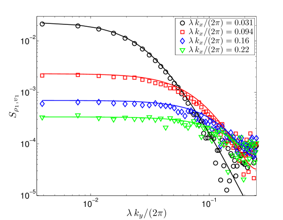
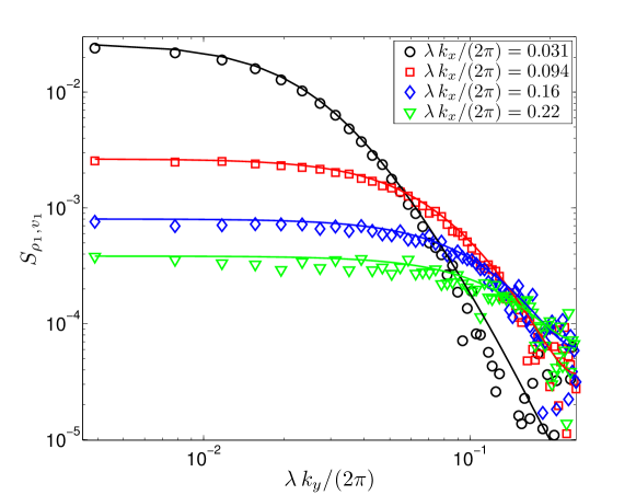
Figure 3: (Top) Discrete structure factor $\mathcal{S}_{\rho_{1},v_{\|}^{(1)}}$ from quasi two-dimensional DSMC runs with $L_{x}=64\lambda$, $L_{y}=512\lambda$ and $L_{z}=2\lambda$, for several wavenumbers $k_{x}=\kappa_{x}\cdot 2\pi/L_{x}$ (circles $\kappa_{x}=2$, squares $\kappa_{x}=6$, diamonds $\kappa_{x}=10$, triangles $\kappa_{x}=14$), compared to $\bar{\rho}S_{c,v_{\|}}$ (solid lines of the same color) as predicted by the linearized periodic theory (10,16). The sides of the DSMC collision cells are $\Delta x_{c}=\Delta y_{c}=2\lambda=7.5$. Note that for a fixed $k_{x}$ we expect the structure factor to decay as $k_{y}^{-4}$. (Bottom) All the parameters, including the system and sampling cell size, are as for the system in the top panel, but now the DSMC cells are twice smaller, $\Delta x_{c}=\Delta y_{c}=\lambda=3.75$. Note that this change of the DSMC cell size changes the kinetic theory prediction for viscosity by more than 20% DSMC_CellSizeError .

In Fig. 3 we compare the theoretical prediction for $\bar{\rho}S_{c,v_{\|}}(\boldsymbol{\kappa})$ to results from particle simulations for the discrete structure factor

$$\mathcal{S}_{\rho_{1},v_{\|}^{(1)}}(\boldsymbol{\kappa})=\left\langle\left(\widehat{\delta\rho_{1}}\right)\left(\widehat{\delta v}_{\|}^{(1)}\right)^{\star}\right\rangle,$$

for two different sizes of the DSMC collision cells. The fact that there is little difference between the two panels in the figure verifies that the details of the microscopic collision dynamics do not affect the mesoscopic hydrodynamic behavior. In Fig. 4 we plot the discrete structure factor from the particle simulations for wavevectors perpendicular to the gradient (i.e., $k_{y}=0$), for systems of different width $L_{x}$.

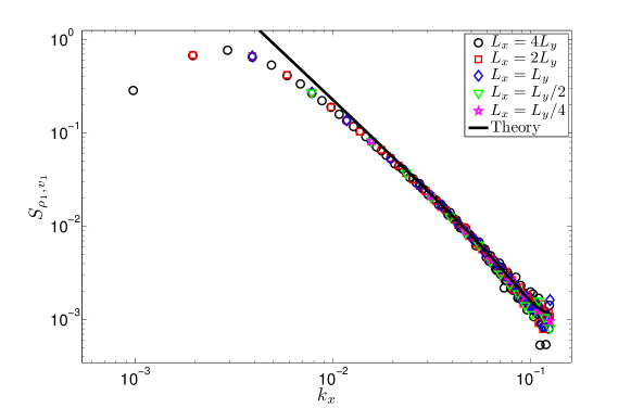
Figure 4: Discrete structure factor $\mathcal{S}_{\rho_{1},v_{\|}^{(1)}}$ from quasi two-dimensional DSMC runs with $L_{y}=512\lambda$ and $L_{z}=\Delta x_{c}=\Delta y_{c}=2\lambda$, for wavevectors perpendicular to the gradient ($k_{y}=0$). Results for systems of different width $L_{x}$ are shown with symbols (see legend). For comparison, the theoretical prediction for $\bar{\rho}S_{c,v_{\|}}$ for an infinite periodic system (10,16) is shown with a line. Deviations from the predicted $k_{x}^{-2}$ power-law divergence are clear for $k_{x}\lesssim 2\pi/L_{y}\approx 3\cdot 10^{-3}$ due to the influence of the top and bottom walls.

It is expected that compressibility effects would affect $\mathcal{S}_{\rho_{1},v_{\|}^{(1)}}$. Indeed, this is what we observe in simulations, however, as Fig. 3 demonstrates, the incompressible isothermal theory for $\bar{\rho}S_{c,v_{\|}}$ is in very good agreement with particle data for $\mathcal{S}_{\rho_{1},v_{\|}^{(1)}}$. Good agreement between the simulation data and the simple theory is also seen in Fig. 4, except for $k_{x}$ comparable to $2\pi/L_{y}$. As expected, for the smallest wavenumbers the top and bottom walls intervene and the actual correlation is smaller than the predicted $k_{x}^{-2}$ divergence.

In order to construct a theoretical prediction for $\mathcal{S}_{\rho_{1},v_{\|}^{(1)}}$, one must not only include the effects of compressibility but also replace the “one-fluid” approximation (3) with a corresponding “two-fluid” compressible hydrodynamic theory BinaryMixKineticTheory ; MultiFluidKineticTheory . This can be seen by noting that the fluctuating equations (3) assume that relation (1) applies to the fluctuating $\boldsymbol{v}_{12}$ and $c$ instead of their means. Such an assumption leads to unphysical bias of order $\left\langle\left(\delta c\right)^{2}\right\rangle$ in the mean inter-species velocity $\left\langle\boldsymbol{v}_{12}\right\rangle$ because of the nonlinearity in the denominator $c(1-c)$. In fact, the fluctuations $\delta\boldsymbol{v}_{12}$ and $\delta c$ should be uncorrelated, as seen from a two-fluid fluctuating theory. Here we use the incompressible isothermal approximation for $\bar{\rho}S_{c,v_{\|}}$ as a proxy for $\mathcal{S}_{\rho_{1},v_{\|}^{(1)}}$ in order to construct theoretical predictions for the diffusion enhancement.

III.2 Fluctuation-Enhanced Diffusion Coefficient

As we already explained, instantaneous hydrodynamic quantities, denoted with a subscript $\Delta\mathcal{V}$, are sampled from the particle data by taking snapshots of the particle state using a grid of sampling cells of volume $\Delta V$. The ensemble average of a given quantity, which we will denote with angle brackets, is obtained by averaging over many snapshots once a steady state is reached, and additional averaging can be performed over all sampling cells with the same $y$ position since the steady state averages cannot depend on $x$ and $z$. We estimate the macroscopic mean mass density $\bar{\rho}$, partial density $\bar{\rho}_{1}$, partial momentum density $\bar{\boldsymbol{j}}_{1}$, partial velocity $\bar{\boldsymbol{v}}_{1}$ and concentration $\bar{c}$ as

$$\bar{\rho}=\rho_{0}=\left\langle\rho_{\Delta\mathcal{V}}\right\rangle,\quad\bar{\rho}_{1}=\left\langle\rho_{\Delta\mathcal{V}}^{(1)}\right\rangle=\bar{c}\bar{\rho}\mbox{ and }\bar{\boldsymbol{j}}_{1}=\boldsymbol{j}_{0}^{(1)}=\left\langle\boldsymbol{j}_{\Delta\mathcal{V}}^{(1)}\right\rangle=\bar{\rho}_{1}\bar{\boldsymbol{v}}_{1}.$$

We also define the mesoscopic velocity and concentrations to be the ensemble averages of the instantaneous values,

$$\boldsymbol{v}_{0}^{(1)}=\left\langle\boldsymbol{v}_{\Delta\mathcal{V}}^{(1)}\right\rangle\mbox{ and }c_{0}=\left\langle c_{\Delta\mathcal{V}}\right\rangle,$$

where the subscript zero will be used to simplify the cumbersome notation. It is important to point out that for non-conserved quantities such as $\boldsymbol{v}$ and $c$ the mesoscopic mean can be different from the macroscopic mean due to fluctuations Tysanner:04 ; UnbiasedEstimates_Garcia , $\bar{\boldsymbol{v}}_{1}\neq\boldsymbol{v}_{0}^{(1)}$ and $\bar{c}\neq c_{0}$. For conserved quantities (e.g., $\bar{\boldsymbol{j}}_{1}$ and $\boldsymbol{j}_{0}^{(1)}$), however, the mesoscopic and macroscopic ensemble means are equal and in fact independent of $\Delta x$ and $\Delta z$ (but not necessarily $\Delta y$).

In particle simulations, we calculate the effective diffusion coefficient $\chi_{\text{eff}}$ from the momentum density of one of the species along the vertical direction,

$$\bar{j}_{\parallel}^{(1)}=\rho_{0}\chi_{\text{eff}}\,\frac{\bar{c}_{T}-\bar{c}_{B}}{L_{y}-\Delta y}\approx\rho_{0}\chi_{\text{eff}}\,\nabla\bar{c},$$ (18)

where we measure $\bar{c}_{T}$ and $\bar{c}_{B}$ in the top and bottom layer of sampling cells (whose centers are a distance $L_{y}-\Delta y$ from each other) to empirically account for the small concentration slip in DSMC (about $0.5\%$ with these parameters). Numerical experiments have verified that $\bar{j}_{\parallel}^{(1)}$ matches the flux obtained from counting the average number of color flips at the top or bottom walls. Furthermore, the results verify that $\chi_{\text{eff}}$ is essentially independent of the magnitude of the concentration gradient, and that the change in the effective gradient $\nabla\bar{c}$ as $L_{x}$ or $L_{z}$ is changed, keeping $L_{y}$ fixed, is much smaller than the change in $\chi_{\text{eff}}$.

The traditional definition of a “renormalized” diffusion coefficient DiffusionRenormalization_I ; DiffusionRenormalization_II as the macroscopic limit of $\chi_{\text{eff}}$, only works in three dimensions and is not very useful for confined systems. Instead, for each sampling cell, we define a locally renormalized diffusion coefficient $\chi_{0}$ via

$$\rho_{0}^{(1)}\boldsymbol{v}_{0}^{(1)}=\left\langle\rho_{\Delta\mathcal{V}}^{(1)}\right\rangle\left\langle\boldsymbol{v}_{\Delta\mathcal{V}}^{(1)}\right\rangle=\bar{\rho}\chi_{0}\left(\boldsymbol{\nabla}\bar{c}\right),$$ (19)

where we have accounted for the fact that the macroscopic concentration gradient $d\bar{c}/dy$ may depend on $y$. In fact, such a dependence is observed in the particle simulations, and we have approximated the local concentration gradient $d\bar{c}/dy$ by a numerical derivative of a polynomial fit of degree five to $\bar{c}(y)$. Figure 5 shows that the empirical $\chi_{0}$ is independent of $y$, except for a boundary layer close to the top and bottom walls. This is an important finding, since (19) is a constitutive model that is assumed to hold not just at the macroscale but also at the mesoscale, notably, $\chi_{0}$ is an input parameter for fluctuating hydrodynamics finite-volume solvers LLNS_S_k .

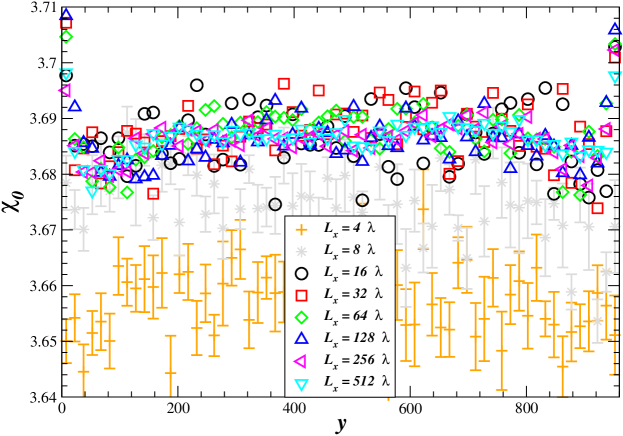
Figure 5: The renormalized diffusion coefficient $\chi_{0}$, as defined by Eq. (19), as a function of the $y$ position of the sampling cell for DSMC systems with several system widths $L_{x}$. The estimate of $\chi_{0}$ shown in Fig. 6 is simply the average over all sampling cells further than $10\Delta y$ away from the top and bottom walls.

Figure 6a shows how the effective $\chi_{\text{eff}}$ and renormalized $\chi_{0}$ diffusion coefficients change as the width of the system $L_{x}$ is increased while keeping the height $L_{y}$ fixed for two different quasi two-dimensional DSMC systems. For System A, the DSMC collision cells are cubes of side $\Delta x_{c}=7.5=2\lambda$, while each sampling cell contains $2\times 2\times 1$ collision cells, or $N_{p}=101$ particles on average. The height of the box is $L_{y}=256\lambda=960$ and the imposed concentrations at the walls are $c_{B}=0.25$ and $c_{T}=0.75$. For System B, the DSMC parameters and $c_{T/B}$ are the same as for to System A, but the sampling cells are twice as large, $4\times 4\times 1$ collision cells each, and the system height is twice as large, $L_{y}=512\lambda=1920$. We obtain similar results using twice smaller collision cells (not shown). For the quasi two-dimensional systems, the thickness is $L_{z}=7.5=2\lambda$ and there is only one DSMC collision cell along the $z$ direction. Figure 6a shows that $\chi_{\text{eff}}$ grows like $\ln L_{x}$, with a slope that is well-predicted by Eq. (14). For widths larger than about $8$ mean free paths, $\chi_{0}$ becomes constant and rather similar to the kinetic theory prediction. It is important to point out that $\chi_{0}$ is not a fundamental material constant and in fact depends on the shape of the sampling cells (see Section III.2.2).

In Fig. 6b we show results from three dimensional DSMC simulations, in which the system width ($x$) and depth ($z$) directions are equivalent, $L_{z}=L_{x}=L$, and the rest of the parameters are the same as for System A. Similar behavior is seen as in two dimensions, except that now the effective diffusion grows as $-L^{-1}$ and saturates to a constant value for large $L$, assuming that $L_{y}\gg L$.

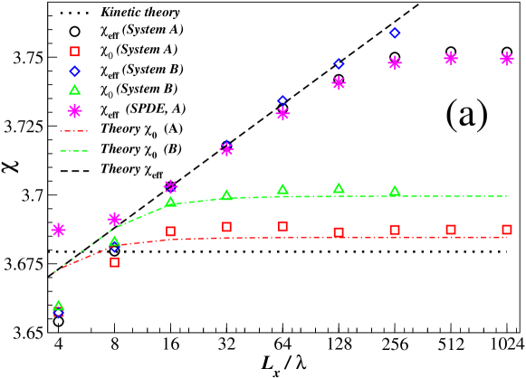
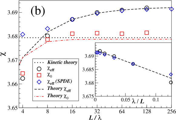
Figure 6: (Panel a, top) The effective $\chi_{\text{eff}}$ and the renormalized $\chi_{0}$ diffusion coefficients as a function of the width of the system $L_{x}$ in two dimensions. Numerical results for System A (DSMC and SPDE) and System B (DSMC) are shown with symbols (see legend). The error bars for all of the numerical data are comparable or smaller than the size of the symbols. The theoretical predictions (23) are evaluated numerically and shown with lines. The bare diffusion in the theory and SPDE calculations is adjusted so that for $L_{x}=16\lambda$ the effective diffusion is the same as that measured in the particle simulations. (Panel b, bottom) Same as the top panel but in three dimensions. The inset highlights the $L^{-1}$ behavior.

III.2.1 Corrections due to finite height

The predictions of the simplified fluctuating hydrodynamic theory, Eqs. (14) and (15), are shown in Fig. 6 and seen to be in very good agreement with the particle simulations for intermediate $L_{x}$. However, the particle data shown in Fig. 6a shows measurable deviations from the simple theory for $L_{x}\gtrsim L_{y}/2$. To understand the discrepancy, recall that the incompressible isothermal theory assumed that $L_{y}$ is essentially infinite and thus in two dimensions $\chi_{\text{eff}}$ grows unbounded in the macroscopic limit. A scaling analysis suggests a modification of (14) to account for the finite height of the system,

$$\chi_{\text{eff}}^{(2D)}\approx\chi+\frac{k_{B}T}{4\pi\rho(\chi+\nu)L_{z}}\,\left[\ln\frac{L_{x}}{L_{0}}-f(r)\right],$$ (20)

where $r=L_{x}/L_{y}$ is the aspect ratio of the system, and $f(r)$ is some function that is close to zero for small $r$ and grows asymptotically as $\ln(r)$. Therefore, when $L_{x}\gg L_{y}$, $\chi_{\text{eff}}$ saturates to a constant value that grows as $\ln(L_{y}/L_{0})$.

One can extend the theoretical calculations to account for the hard wall boundary conditions in the $y$ direction FluctHydroNonEq_Book , however, such a calculation is non trivial. Instead, we have used the finite-volume solver developed in Ref. LLNS_S_k to solve the non-linear system of SPDEs (3) for the same system dimensions as in the particle simulations. The results, shown in Fig. 6, are in excellent agreement with the particle simulations for the larger system sizes. Note that while our SPDE solver includes all of the nonlinear terms in (3), we may artificially reduce the amplitude of the noise and thus the magnitude of the fluctuations by some factor $\epsilon\ll 1$. This reduces the effect of the nonlinearities and effectively gives a quasi-linearized finite-volume SPDE solver. The advective mass flux due to the velocity fluctuations can be estimated as

$$\Delta\bar{j}_{\parallel}^{(1)}(y)\approx\epsilon^{-2}\left\langle\left(\delta\rho_{1}\right)\left(\delta v_{\parallel}^{(1)}\right)\right\rangle\approx\epsilon^{-2}\bar{\rho}\left\langle\left(\delta c\right)\left(\delta v_{\parallel}\right)\right\rangle,$$ (21)

and may depend on $y$ especially close to the walls or when $L_{y}\gtrsim L_{x}$. The sum of the average diffusive and advective mass fluxes must be independent of $y$,

$$\bar{j}_{\parallel}^{(1)}=\bar{\rho}\chi_{\text{eff}}\,\frac{c_{T}-c_{B}}{L_{y}}=\bar{\rho}\chi_{0}\frac{d\bar{c}(y)}{dy}-\Delta\bar{j}_{\parallel}^{(1)}(y),$$ (22)

which implies that the macroscopic concentration profile $\bar{c}(y)$ is affected by the fluctuations as well and cannot be strictly linear. From the conditions $c(0)=c_{B}$ and $c(L_{y})=c_{T}$ and (22) we obtain the relation

$$\chi_{\text{eff}}=\chi_{0}-\left[\bar{\rho}\left(c_{T}-c_{B}\right)\right]^{-1}\;\int_{y=0}^{L_{y}}\left[\Delta\bar{j}_{\parallel}^{(1)}(y)\right]dy,$$

which is how we calculate the effective diffusion coefficient from the numerical SPDE solution. We have verified that the results are independent of $\epsilon$ to within statistical accuracy for $\epsilon\leq 1/2$.

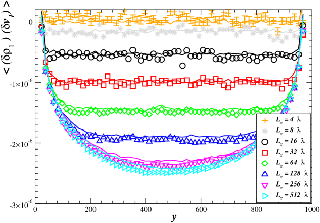
Figure 7: The fluctuating contribution to the mean diffusive flux, $\left\langle\left(\delta\rho_{1}\right)\left(\delta v_{\parallel}^{(1)}\right)\right\rangle$, as a function of the height of the sampling cell $y$, for several system widths $L_{x}$, keeping $L_{y}=256\lambda$. Data from quasi-two dimensional particle simulations (System A) is shown with symbols, and lines of the same color show data for $\bar{\rho}\left\langle\left(\delta c\right)\left(\delta v_{\parallel}\right)\right\rangle$ obtained using a two-dimensional finite-volume solver LLNS_S_k for the LLNS equations (3). The error bars for the particle data are shown for $L_{x}=4\lambda$, and are similar or smaller for the remaining systems and for the finite-volume results.

The velocity-concentration correlation $\Delta\bar{j}_{\parallel}^{(1)}(y)$ obtained from the finite-volume solver is shown in Fig. 7, along with the corresponding particle data for comparison. Excellent agreement is seen, demonstrating that the finite-volume solution correctly accounts for the influence of the boundaries. Note that the partial velocity $\boldsymbol{v}_{1}$ is not included as an independent variable in (3) and the mean velocity $\boldsymbol{v}$ is used instead. When compressibility effects are included, $\boldsymbol{v}$, unlike $\boldsymbol{v}_{1}$, is correlated with $\rho_{1}$ even in one dimension. This makes a direct comparison between the effective diffusion coefficient in the particle and finite-volume simulations difficult. However, the dependence of $\chi_{\text{eff}}$ on system size should be the same in both types of simulations, once the bare transport coefficient is adjusted empirically.

III.2.2 Renormalized Diffusion Coefficient

The renormalized diffusion coefficient $\chi_{0}$ in the Fickian diffusive flux is an input to the SPDE calculations and assumed constant. In our calculations we used the prediction of kinetic theory DSMC_CellSizeError ; DSMC_TimeStepError , also shown in Fig. 6. In finite-volume solvers, the spacing of the computational grid plays the equivalent of the cutoff length $L_{\text{mol}}$, and therefore the effective mass flux depends on the grid spacing. Furthermore, there are numerical grid artifacts in the SPDE solution at length and time scales comparable to the numerical discretization parameters LLNS_S_k . To correct for these errors, we have added a constant to the effective diffusion coefficient obtained from SPDE runs to match $\chi_{\text{eff}}$ from the particle simulations for $L_{x}=L_{0}=16\lambda$. This correction essentially renormalizes $\chi_{0}$ based on the size of the finite-volume hydrodynamic cells.

One can think of $\chi_{0}$ defined via (19) as the fluctuation-renormalized diffusion coefficient at length scales determined by the shape of the sampling or observation volume $\Delta\mathcal{V}$. In this sense, $\chi_{0}$ is the physical-space equivalent of the wavenumber-dependent diffusion coefficient $\chi\left(\boldsymbol{k},\omega=0\right)$ commonly used in linear response theories DiffusionRenormalization_I ; SelfDiffusion_Linearity . A theoretical prediction for $\chi_{0}$ can be obtained by starting from linearized theory for the fluctuating fields $\rho_{1}\left(\boldsymbol{r},t\right)=\bar{\rho}_{1}+\delta\rho_{1}\left(\boldsymbol{r},t\right)$ and $\boldsymbol{v}_{1}\left(\boldsymbol{r},t\right)=\bar{\boldsymbol{v}}_{1}+\delta\boldsymbol{v}_{1}\left(\boldsymbol{r},t\right)$. The instantaneous velocity in a given sampling cell was defined through the instantaneous momentum density $\boldsymbol{j}_{1}=\rho_{1}\boldsymbol{v}_{1}$ averaged over the sampling cell,

$$\left\langle\rho_{\Delta\mathcal{V}}^{(1)}\right\rangle\left\langle\boldsymbol{v}_{\Delta\mathcal{V}}^{(1)}\right\rangle=\bar{\rho}_{1}\left\langle\boldsymbol{v}_{\Delta\mathcal{V}}^{(1)}\right\rangle=\bar{\rho}_{1}\left\langle\frac{\int_{\Delta\mathcal{V}}\rho_{1}\boldsymbol{v}_{1}\,d\boldsymbol{r}}{\int_{\Delta\mathcal{V}}\rho_{1}\,d\boldsymbol{r}}\right\rangle=\left\langle\rho_{\Delta\mathcal{V}}^{(1)}\boldsymbol{v}_{\Delta\mathcal{V}}^{(1)}\right\rangle-\Delta\boldsymbol{j}_{F},$$

where to second order in the fluctuations,

$$\Delta\boldsymbol{j}_{F} =\Delta V^{-2}\int_{\Delta\mathcal{V}}d\boldsymbol{r}\,\int_{\Delta\mathcal{V}}d\boldsymbol{r}^{\prime}\,\left\langle\rho_{1}(\boldsymbol{r},t)\boldsymbol{v}_{1}(\boldsymbol{r}^{\prime},t)\right\rangle$$

$$= \Delta V^{-2}\int_{\Delta\mathcal{V}}d\boldsymbol{r}\,\int_{\Delta\mathcal{V}}d\boldsymbol{r}^{\prime}\;\left(2\pi\right)^{-6}\int_{\boldsymbol{k}}d\boldsymbol{k}\int_{\boldsymbol{k}^{\prime}}d\boldsymbol{k}^{\prime}\;\left\langle\widehat{\delta\rho_{1}}\left(\boldsymbol{k},t\right)\widehat{\delta\boldsymbol{v}_{1}}^{\star}\left(\boldsymbol{k}^{\prime},t\right)\right\rangle e^{i\left(\boldsymbol{k}\cdot\boldsymbol{r}-\boldsymbol{k}^{\prime}\cdot\boldsymbol{r}^{\prime}\right)}$$

$$= \left(2\pi\right)^{-3}\int_{\boldsymbol{k}}\left[\Delta V^{-2}\int_{\Delta\mathcal{V}}d\boldsymbol{r}\,\int_{\Delta\mathcal{V}}d\boldsymbol{r}^{\prime}\,e^{i\boldsymbol{k}\cdot\left(\boldsymbol{r}-\boldsymbol{r}^{\prime}\right)}\right]\mathcal{S}_{\rho_{1},\boldsymbol{v}_{1}}\left(\boldsymbol{k}\right)\,d\boldsymbol{k}$$

$$= \left(2\pi\right)^{-3}\int_{\boldsymbol{k}}F_{\Delta\mathcal{V}}\left(\boldsymbol{k}\right)\,\mathcal{S}_{\rho_{1},\boldsymbol{v}_{1}}\left(\boldsymbol{k}\right)\,d\boldsymbol{k},$$

and $F_{\Delta\mathcal{V}}\left(\boldsymbol{k}\right)$ is the low pass filter that already appeared in Eq. (17). The result of this calculation [c.f. Eq. (12)],

$$\chi_{\text{eff}} =\chi-\left(2\pi\right)^{-3}\int_{\boldsymbol{k}}\left[\rho_{0}^{-1}\Delta\mathcal{S}_{\rho_{1},v_{\|}^{(1)}}\left(\boldsymbol{k}\right)\right]\,d\boldsymbol{k}$$

$$\chi_{0} =\chi-\left(2\pi\right)^{-3}\int_{\boldsymbol{k}}\left[1-F_{\Delta\mathcal{V}}\left(\boldsymbol{k}\right)\right]\left[\rho_{0}^{-1}\Delta\mathcal{S}_{\rho_{1},v_{\|}^{(1)}}\left(\boldsymbol{k}\right)\right]\,d\boldsymbol{k},$$ (23)

shows that $\chi_{\text{eff}}$ includes contributions from all wavenumbers present in the system, while $\chi_{0}$ only includes “sub-grid” contributions, from wavenumbers larger than $2\pi/\Delta x$. The theoretical predictions shown in Fig. 6 are based on numerically evaluating (23) after replacing the integrals over $k_{x}$ and $k_{z}$ (23) with the appropriate sums, assuming $\mathcal{S}_{\rho_{1},\boldsymbol{v}_{1}}\approx\bar{\rho}\mathcal{S}_{c,\boldsymbol{v}}$ and using Eq. (10). The bare diffusion coefficient $\chi$ is adjusted so that $\chi_{\text{eff}}$ matches the particle result for $L_{x}=L_{0}=16\lambda$, and good agreement is observed between (23) and the particle data for $\chi_{0}$ for all but the smallest $L_{x}$.

While it is intuitive to expect that the bare diffusion coefficient should account for molecular, or non-hydrodynamic, degrees of freedom, the division $\chi_{\text{eff}}=\chi+\Delta\chi$ is arbitrary, and in fact there is no unambiguous way to define $\chi$. This is evident in the theory because of the need to introduce an ad-hoc molecular cutoff as a way to separate the “microscopic” from the “mesoscopic” scales. By contrast, the locally renormalized diffusion coefficient $\chi_{0}$ defined in (19) explicitly depends on the size of the sampling (hydrodynamic) cells $\Delta V=\left|\Delta\mathcal{V}\right|$ used to define the hydrodynamic quantities from the particle configuration. Combining the two equations in (23) gives the renormalization relation at large scales,

$$\chi_{\text{eff}}=\chi_{0}\left(\Delta\mathcal{V}\right)-\left(2\pi\right)^{-3}\int_{\boldsymbol{k}}F_{\Delta\mathcal{V}}\left(\boldsymbol{k}\right)\left[\rho_{0}^{-1}\Delta\mathcal{S}_{\rho_{1},v_{\|}^{(1)}}\left(\boldsymbol{k}\right)\right]d\boldsymbol{k},$$

which eliminates the dependence on the ad-hoc cutoff wavenumber since $F_{\Delta\mathcal{V}}$ filters contributions from large wavenumbers, at least within the simple perturbative (quasi-linear) theory.

IV Connections to Earlier Work

While our computer simulations are the first hydrodynamic study of the dependence of transport on system size, there is a substantial body of literature that has discussed the effect from a theoretical perspective or studied smaller particle systems. In this section we explicitly connect our analysis to previous approaches, and discover direct relations with work that might have, at first sight, been assumed to be unrelated.

IV.1 Relation to Long-Time Tails

It is well known that the self-diffusion coefficient is given by the integral of the equilibrium velocity autocorrelation function (VACF) $C(t)$ of the fluid particles LongRangeCorrelations_MD . The long-time tail of $C(t)$ has been extensively studied in the literature both computationally and through several theories, including heuristic hydrodynamic arguments Alder:70 ; VACFTail_Widom , kinetic theory VACFTail_Cohen and (second-order) mode-mode coupling hydrodynamic theory ModeModeCoupling . Ultimately all derivations give the same result including not just the power-law dependence but also the coefficient of the tail, specifically, in three dimensions $C(t)\approx k_{B}T/\left\{12\rho\left[\pi\left(\chi+\nu\right)t\right]^{3/2}\right\}$, while for quasi-two dimensional systems $C(t)\approx k_{B}T/\left[8\pi\rho L_{z}\left(\chi+\nu\right)t\right]$.

A crucial point is that the VACF explicitly depends on the system size due to periodic boundaries, and so its integral, which gives the diffusion coefficient, also depends on system size. More explicitly, ignoring acoustic effects, the VACF has the power-law dependence only for $L_{\text{mol}}^{2}/\left(\chi+\nu\right)\ll t\ll L^{2}/\left(\chi+\nu\right)$, and it decays exponentially for large times BrownianParticle_SIBM . Ignoring prefactors, the contribution of the tail to the diffusion coefficient in three dimensions is estimated as

$$\Delta\chi_{\text{tail}}\sim\int_{L_{\text{mol}}^{2}/\left(\chi+\nu\right)}^{L^{2}/\left(\chi+\nu\right)}\frac{k_{B}T}{\rho\left[\left(\chi+\nu\right)t\right]^{3/2}}dt\sim\frac{k_{B}T}{\rho\left(\chi+\nu\right)}\left(\frac{1}{L_{\text{mol}}}-\frac{1}{L}\right),$$ (24)

which of exactly the same form as (15). A similar calculation in two dimensions reproduces the logarithmic dependence in (14).

A more quantitative comparison to the theories for the VACF tail can be made by examining the predictions of the mode-mode coupling theory for the long-time tail, reviewed in detail in Section 3.2 of Ref. ModeModeCoupling . The relevant formula for the VACF is their Eq. (3.39), which, after integrating over the Boltzmann velocity distribution, becomes

$$C(t)=\frac{k_{B}T}{12\pi^{3}\rho}\int_{\boldsymbol{k}}\exp\left[-\left(\chi+\nu\right)k^{2}t\right]d\boldsymbol{k}.$$

In ModeModeCoupling , the integral over $\boldsymbol{k}$ is performed assuming an infinite system and the time dependence kept in order to see the behavior of the tail at long times. If we integrate over $t$ instead, we get

$$\Delta\chi_{\text{tail}}=\int_{t=0}^{\infty}C(t)dt=\frac{k_{B}T}{12\pi^{3}\rho(\chi+\nu)}\int_{\boldsymbol{k}}k^{-2}d\boldsymbol{k},$$ (25)

which is seen to identical to the integral in Eq. (12) under the assumption that all three directions $x$, $y$ and $z$ are identical (as done in all VACF calculations),

$$\Delta\chi=\frac{k_{B}T}{(2\pi)^{3}\rho\left(\chi+\nu\right)}\;\int_{\boldsymbol{k}}\frac{k_{x}^{2}+k_{z}^{2}}{k^{4}}\,d\boldsymbol{k}=\frac{k_{B}T}{(2\pi)^{3}\rho\left(\chi+\nu\right)}\;\frac{2}{3}\int_{\boldsymbol{k}}k^{-2}\,d\boldsymbol{k}=\Delta\chi_{\text{tail}}.$$

Note that for a finite system one ought to replace the integrals over $\boldsymbol{k}=\boldsymbol{\kappa}\cdot 2\pi/L$ with sums over $\boldsymbol{\kappa}\in Z^{d}$ that exclude $\boldsymbol{\kappa}=0$,

$$\Delta\chi_{\text{tail}}=\frac{2k_{B}T}{3\rho(\chi+\nu)L^{3}}\sum_{\boldsymbol{\kappa}\neq\boldsymbol{0}}k^{-2}.$$ (26)

In the Molecular Dynamics (MD) literature, the dependence on $L^{-1}$ in Eq. (24) is considered a finite-size effect that ought to be removed in order to extract the bulk ($L\rightarrow\infty$) limit of the diffusion coefficient TracerDiffusion_HS ; SelfDiffusionFinite_HS ; FiniteSize_Diffusion_MD . A hydrodynamic theory for the finite-size correction, based on the Oseen tensor for a finite periodic system, has been developed several times PolymerChainMD_Dunweg and is confirmed numerically in Refs. FiniteSize_Diffusion_MD . This theory focuses on viscous effects only, and we will thus replace $\nu$ with $\nu+D$ in Eqs. (10,11) in Ref. FiniteSize_Diffusion_MD , to obtain

$$\Delta\chi_{\text{MD}}=\frac{k_{B}T}{6\pi\left(\chi+\nu\right)}\left[\tilde{f}(k_{\max})+\sum_{\boldsymbol{\kappa}\neq\boldsymbol{0}}4\pi L^{-3}k^{-2}\exp\left(-\frac{k^{2}}{4k_{\max}^{2}}\right)\right],$$

where $\tilde{f}(k)$ is some function. Assuming that $k_{\max}$ is large, the system-size dependence is captured in the last term, which is exactly the same as Eq. (26),

$$\Delta\chi_{\text{MD}}\approx\frac{k_{B}T}{6\pi\left(\chi+\nu\right)}\sum_{\boldsymbol{\kappa}\neq\boldsymbol{0}}4\pi L^{-3}k^{-2}=\Delta\chi_{\text{tail}}=\Delta\chi.$$

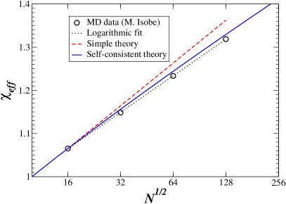
Figure 8: System-size dependence of the diffusion coefficient for hard disks at volume fraction $\phi=0.18$ (data courtesy of Masaharu Isobe VACF_2D_HS ). Time and lengths are measured in natural units, or, equivalently, $k_{B}T=1$, $m=1$ and disk diameter $\sigma=1$. (Left) The time-dependent diffusion coefficient $\chi(t)$, as determined from a numerical integral of the velocity autocorrelation function, for several system sizes (see legend). (Right) The observed increase of the effective diffusion coefficient with system size (symbols), as obtained from the large-time limit of $\chi(t)$. Theoretical predictions are shown for comparison, for both the simple theory (27) (dashed line), as well as for the self-consistent theory (29) with the system size $N_{0}=16^{2}$ used to define a reference length $L_{0}$. A logarithmic fit with an adjustible slope is also shown (dotted line).

There are few molecular dynamics studies of the system size dependence of the diffusion coefficient in sufficiently large two-dimensional systems. Isobe has performed one of the most extensive hard-disk molecular dynamics studies of the hydrodynamic tail of the VACF VACF_2D_HS . We have performed numerical integration of $C(t)$ using the data of Isobe for hard disks at packing fraction $\phi=0.18$, for square systems sizes containing from $N=16^{2}$ to $N=128^{2}$ hard disks. For these parameters the statistical accuracy of the data appears sufficient to resolve the asymptotic plateau $\chi_{\text{eff}}=\lim_{\tau\rightarrow\infty}\chi(t)$ of the time-dependent diffusion coefficient

$$\chi(t)=\int_{\tau=0}^{t}C(\tau)d\tau,$$

as illustrated in Fig. 8. Since the aspect ratio of all of Isobe’s simulations is fixed at $L_{x}/L_{y}=1$, Eq. (20) suggests that the difference between $\chi_{\text{eff}}$ for a system size of $N$ disks and the smallest system of $N_{0}=16$ disks is

$$\chi_{\text{eff}}(N)-\chi_{\text{eff}}(N_{0})\approx\frac{k_{B}T}{8\pi\rho(\chi+\nu)}\,\ln\frac{N}{N_{0}}.$$ (27)

In Fig. 8 we compare this prediction to the numerical integral of Isobe’s data, using Enskog kinetic theory Enskog_2DHS values for the “bare” transport coefficients $\chi$ and $\nu$ of the hard disk fluid at this density. Good agreement is observed, demonstrating that the effect we observe is not an artifact of DSMC but rather a generic property of fluids.

IV.2 Self-Consistent Theory

The theoretical predictions with which we compared the particle results were based on a leading-order perturbative theory DiffusionRenormalization_I that relies on the solution of the linearized equations of fluctuating hydrodynamics. A fully nonlinear theory, however, remains illusive. In the context of infinite (bulk) systems, a systematic perturbative theory that accounts for corrections of order higher than quadratic in the fluctuations has been discussed in Refs. DiffusionRenormalization_II ; TrilinearModeCoupling . In three dimensions, the conclusion of such studies has been that the higher-order terms do not affect the form of (23). In two dimensions, several calculations VACF_2D_SelfConsistentMC ; TrilinearModeCoupling ; SCModeModeCoupling2D and numerical simulations VACF_2Divergence ; VACF_2D_HS suggest that including higher-order terms changes the logarithmic growth in (14). Specifically, it has been predicted that the self-consistent power-law decay for the VACF is faster than $t^{-1}$, $C(t)\sim\left(t\sqrt{\ln t}\right)^{-1}$, which changes the asymptotic growth of $\chi_{\text{eff}}$ from $\ln L_{x}$ to $\sqrt{\ln L_{x}}$.

In order to obtain a self-consistent form of (14), we reconsider the derivation in Section II.1.1. The cause of the diffusion growth from system width $L_{x}$ to $L_{x}+dL_{x}$ is the added contribution to the integral in Eq. (13) from wavenumbers in the band $\left|k_{x}\right|\in 2\pi L_{x}^{-1}\cdot\left[1-dL_{x}/L_{x},1\right]$. If we postulate that the concentration fluctuations at wavenumber $k_{x}=2\pi/L_{x}$ evolve with the renormalized diffusion coefficient $\chi_{\text{eff}}\left(L_{x}\right)$, instead of the bare one, we obtain an ordinary differential equation for $\chi_{\text{eff}}\left(L_{x}\right)$,

$$\frac{d\chi_{\text{eff}}}{dL_{x}}\approx\frac{k_{B}T}{(2\pi)^{2}\rho\left(\chi_{\text{eff}}+\nu\right)L_{z}}\left(2\,\frac{k_{x}}{L_{x}}\right)\int_{k_{y}}\frac{k_{x}^{2}}{\left(k_{x}^{2}+k_{y}^{2}\right)^{2}}\,dk_{y}=\frac{k_{B}T}{4\pi\rho(\chi_{\text{eff}}+\nu)L_{z}}L_{x}^{-1},$$ (28)

where we have assumed that viscosity does not change substantially with system size (consistent with existing molecular dynamics data). Solving the differential equation (28) with the condition $\chi_{\text{eff}}\left(L_{0}\right)=\chi$ leads to a diffusion enhancement that grows slightly slower than logarithmically,

$$\chi_{\text{eff}}\left(L_{x}\right)\approx\left(\chi+\nu\right)\left[1+\frac{k_{B}T}{2\pi\rho(\chi+\nu)^{2}L_{z}}\,\ln\frac{L_{x}}{L_{0}}\right]^{1/2}-\nu.$$ (29)

Although the self-consistent form (29) still diverges with system length, it is important to observe that for any finite system $\chi_{\text{eff}}$ is well-defined. The predictions of (29) for a hard-disk system at packing fraction $\phi=0.18$ are shown in Fig. 8. We have used the Enskog kinetic theory for the viscosity, which is in good agreement with published molecular dynamics data at this density, and set $\rho L_{z}$ to be the mass density in the plane. The self-consistent theory is seen to be in better agreement with the molecular dynamics data than the simple theory (14); however, the difference between the two is small for the system sizes at which we presently have reliable data for the effective diffusion coefficient.

Repeating the same self-consistent calculation in three dimensions gives the self-consistent form,

$$\chi_{\text{eff}}\left(L\right)\approx\left(\chi+\nu\right)\left[1+\frac{\alpha\,k_{B}T}{\rho(\chi+\nu)^{2}}\left(\frac{1}{L_{0}}-\frac{1}{L}\right)\right]^{1/2}-\nu,$$ (30)

which happens to be the solution of the consistency condition

$$\chi_{\text{eff}}=\chi+\frac{\alpha\,k_{B}T}{\rho\left[\nu+(\chi+\chi_{\text{eff}})/2\right]}\left(\frac{1}{L_{0}}-\frac{1}{L}\right),$$

reminiscent of the form obtained in Ref. DiffusionRenormalization_II except that the arithmetic average of $\chi$ and $\chi_{\text{eff}}$ appears in the denominator instead of just $\chi_{\text{eff}}$. In three dimensions, the difference between the self-consistent (30) and the simple (15) theories is very small and thus rather difficult to observe computationally.

In both two and three dimensions, the self-consistent predictions (29,30) will only deviate from the simple theory (14,15) substantially when the diffusion enhancement becomes comparable to the bare coefficient, that is, when hydrodynamic effects become comparable to molecular ones. The estimates presented in Appendix A show that reaching the regime where $\Delta\chi\gtrsim\chi$ is difficult to achieve with particle simulations. In nonlinear fluctuating hydrodynamics finite-volume solvers LLNS_S_k , one has the freedom to choose the various parameters so as to make the effect of advection by velocity fluctuations much more prominent, similarly to what is done in Ref. VACF_2Divergence using a two-dimensional lattice gas method. Experimentally, two dimensional systems can be realized by using thin films, for example, liquid or liquid crystal films. In liquid films, however, velocity fluctuations below a certain cutoff wavenumber are suppressed because of the drag by the surrounding fluid, and therefore the diffusion enhancement saturates for systems much larger than the cutoff length scale GiantFluctuations_ThinFilms .

V Conclusions and Future Directions

The results of our particle simulations confirm that fluctuating hydrodynamics is a powerful tool for understanding transport at small scales. Our results conclusively demonstrate that the advection by thermal velocity fluctuations affects the mean transport in nonequilibrium finite systems and thus the advective nonlinearities, such as the term $\left(\delta c\right)\left(\delta\boldsymbol{v}\right)$ in (5), ought to be retained in the equations of fluctuating hydrodynamics. We demonstrated explicitly that the correction to the bare or molecular transport coefficients due to the VACF tail LongRangeCorrelations_MD , hydrodynamic interactions with periodic images of a given particle FiniteSize_Diffusion_MD , and the contribution due to thermal fluctuations DiffusionRenormalization_I ; ExtraDiffusion_Vailati studied here, are all the same physical phenomenon simply calculated through different theoretical approaches, all of which are equivalent because of linearity. The advantage of fluctuating hydrodynamics is that it is simple, and it can take into account the proper boundary conditions and exact geometry, especially if a numerical SPDE solver is used. Furthermore, other effects such as gravity ExtraDiffusion_Vailati , temperature variations TemperatureGradient_Cannell , or time dependence GiantFluctuations_Theory ; GiantFluctuations_ThinFilms , can easily be included. It remains as a future challenge to verify the predictions of fluctuating hydrodynamics for the effect of fluctuations on diffusive transport in spatially non-uniform systems, either through particle simulations or laboratory experiments GiantFluctuations_ThinFilms .

Renormalization has often been invoked as a way to fold the contribution from fluctuations into the effective transport coefficients, however, this only works in three dimensions for very large systems. In two dimensions, a macroscopic limit does not exist, and in three dimensions there are strong finite-size corrections even for systems with dimensions much larger than molecular scales. Theoretical modeling of finite systems at the nano or microscale thus requires including nonlinear hydrodynamic fluctuations. However, a complete nonlinear theory has yet to be developed, and requires detailed understanding of the role of large wavenumber cutoffs (regularizations) that are necessary to make the SPDEs well-behaved. Furthermore, the proper physical and mathematical interpretation of other types of nonlinearities in (3) and (6,7), notably the dependence of the transport coefficients and the stochastic forcing amplitude on the fluctuations, remain to be clarified. Future work should also study momentum and heat transfer in steady states, as well as time-dependent transport in systems that are far from equilibrium.

Appendix A Estimates of the Diffusion Enhancement

It is instructive to do some scaling analysis of the order of magnitude of $\Delta\chi$ in realistic fluid systems. Following (15), the hydrodynamic contribution to the diffusion coefficient for a large three dimensional system is estimated as

$$\Delta\chi\sim\frac{k_{B}T}{\rho(\chi+\nu)L_{\text{mol}}},$$ (31)

For gases, $\Delta\chi$ can be estimated by using Chapman-Enskog values for the transport coefficients for a hard-sphere gas with molecular collision diameter $\sigma\approx L_{\text{mol}}$, specifically, $\chi\sim\nu\sim\left(\rho\sigma^{2}\right)^{-1}\sqrt{mk_{B}T}$. For liquids, the Schmidt number is large, $S_{c}=\nu/\chi>10^{2}$, and Stokes-Einstein’s relation suggests that $\chi\sim k_{B}T/\left(\rho\nu\sigma\right)$. For both gases and liquids we get that $\Delta\chi/\chi\sim\left(n\sigma^{3}\right)\sim\phi$, where $n=\rho/m$ is the number density and $\phi$ is the packing fraction of the particles. We see from this estimate that the enhancement due to fluctuations is stronger for dense gases and is strongest for liquids.

However, the logarithmic divergence in (14) means that the contribution due to hydrodynamic fluctuations dominates for sufficiently large (quasi) two-dimensional systems, regardless of the density,

$$\frac{\Delta\chi}{\chi}\sim\frac{k_{B}T}{\rho\chi(\chi+\nu)L_{z}}\,\ln\frac{L_{x}}{L_{\text{mol}}}\sim\left(n\sigma^{3}\right)\frac{\sigma}{L_{z}}\,\ln\frac{L_{x}}{\sigma}.$$ (32)

A glance at Fig. 6 shows that the enhancement we measured is only a few percent of the kinetic theory value (for our DSMC simulations, $n\sigma^{3}=0.06$), and reaching the system width $L_{x}$ where $\Delta\chi\sim\chi$ is impractical with DSMC simulations at the present. In fact, for the parameters used in typical DSMC applications the enhancement of the transport coefficients relative to the Chapman-Enskog values is very small. Specifically, assuming an ideal hard-sphere gas collision model and taking $L_{\text{mol}}=\Delta x_{c}$, for a quasi two-dimensional system of thickness $L_{z}=\lambda$ we obtain the estimate

$$\frac{\Delta\chi}{\chi}=\frac{16}{33\pi^{2}\left(n\lambda^{3}\right)}\,\ln N_{x}\approx\left(20N_{\lambda}\right)^{-1}\,\ln N_{x},$$

where $N_{\lambda}=n\lambda^{3}$ is the number of particles per cubic mean free path, and $N_{x}=L_{x}/\Delta x_{c}$ is the number of collision cells along the direction perpendicular to the gradient. In a typical DSMC simulation $N_{\lambda}\approx 100$, giving $\Delta\chi/\chi\approx 0.5\cdot 10^{-3}\,\ln N_{x}$, which is less than $0.5\%$ even for $N_{x}=100$. While using molecular dynamics instead of DSMC allows one to reach larger densities and thus enlarge $\Delta\chi/\chi$, the regime in which $\Delta\chi\gtrsim\chi$ is difficult to access even using hard-disk MD VACF_2D_HS (see Fig. 8).

In this work we focused on the correlations between velocity and concentration fluctuations. Concentration fluctuations also have long ranged self-correlations $\sim k^{-4}$ in the presence of a concentration gradient, see Eq. (9). Even though the enhancement of the concentration fluctuations is proportional to the square of the concentration gradient, a two-dimensional calculation GiantFluctuations_ThinFilms similar to one presented here [see Eqs. (11,13)] leads to the remarkable result,

$$\left\langle\delta c\left(\boldsymbol{r},t\right)\delta c\left(\boldsymbol{r},t\right)\right\rangle_{\text{neq}}^{(2D)}=\frac{3k_{B}T}{128\pi^{3}\rho\chi(\chi+\nu)L_{z}}\,\left(\frac{L_{x}}{L_{y}}\right)^{2}\,\left(\Delta c\right)^{2},$$

where $\Delta c=(\nabla\bar{c})L_{y}$ is the macroscopic concentration variation. Assuming $L_{x}\sim L_{y}$, we thus obtain [c.f. Eq. (32)]

$$\frac{\left\langle(\delta c)(\delta c)\right\rangle_{\text{neq}}^{(2D)}}{\left(\Delta c\right)^{2}}\sim\frac{k_{B}T}{\rho\chi(\chi+\nu)L_{z}}\sim\left(n\sigma^{3}\right)\frac{\sigma}{L_{z}},$$

where $n\sigma^{3}\sim 1$ for liquids. We thus see that for systems a few molecules thick, the non-equilibrium concentration fluctuations can become comparable to the deterministic variation. In this case we expect that a perturbative approach based on the linearized theory will not be applicable and the use of a nonlinear finite-volume solver will be indispensable.

References

- (1) A. L. Garcia, M. Malek Mansour, G. C. Lie, M. Mareschal, and E. Clementi. Hydrodynamic fluctuations in a dilute gas under shear. Phys. Rev. A, 36(9):4348–4355, 1987.
- (2) M. Mareschal, M.M. Mansour, G. Sonnino, and E. Kestemont. Dynamic structure factor in a nonequilibrium fluid: A molecular-dynamics approach. Phys. Rev. A, 45:7180–7183, May 1992.
- (3) J. R. Dorfman, T. R. Kirkpatrick, and J. V. Sengers. Generic long-range correlations in molecular fluids. Annual Review of Physical Chemistry, 45(1):213–239, 1994.
- (4) J.M. Ortiz de Zarate and J.V. Sengers. On the physical origin of long-ranged fluctuations in fluids in thermal nonequilibrium states. J. Stat. Phys., 115:1341–59, 2004.
- (5) J. M. O. De Zarate and J. V. Sengers. Hydrodynamic fluctuations in fluids and fluid mixtures. Elsevier Science Ltd, 2006.
- (6) A. Vailati and M. Giglio. Giant fluctuations in a free diffusion process. Nature, 390(6657):262–265, 1997.
- (7) A. Vailati and M. Giglio. Nonequilibrium fluctuations in time-dependent diffusion processes. Phys. Rev. E, 58(4):4361–4371, 1998.
- (8) D. Brogioli, A. Vailati, and M. Giglio. Universal behavior of nonequilibrium fluctuations in free diffusion processes. Phys. Rev. E, 61(1):1–4, 2000.
- (9) A. Vailati, R. Cerbino, S. Mazzoni, M. Giglio, G. Nikolaenko, C.J. Takacs, D.S. Cannell, W.V. Meyer, and A.E. Smart. Gradient-driven fluctuations experiment: fluid fluctuations in microgravity. Applied Optics, 45(10):2155–2165, 2006.
- (10) F. Croccolo, D. Brogioli, A. Vailati, M. Giglio, and D. S. Cannell. Nondiffusive decay of gradient-driven fluctuations in a free-diffusion process. Phys. Rev. E, 76(4):041112, 2007.
- (11) A. Vailati, R. Cerbino, S. Mazzoni, C. J. Takacs, D. S. Cannell, and M. Giglio. Fractal fronts of diffusion in microgravity. Nature Communications, 2:290, 2011.
- (12) C. J. Takacs, G. Nikolaenko, and D. S. Cannell. Dynamics of long-wavelength fluctuations in a fluid layer heated from above. Phys. Rev. Lett., 100(23):234502, 2008.
- (13) R. Schmitz. Fluctuations in nonequilibrium fluids. Physics Reports, 171(1):1–58, 1988.
- (14) A. Donev, E. Vanden-Eijnden, A. L. Garcia, and J. B. Bell. On the Accuracy of Explicit Finite-Volume Schemes for Fluctuating Hydrodynamics. Communications in Applied Mathematics and Computational Science, 5(2):149–197, 2010.
- (15) D. Brogioli. Giant fluctuations in diffusion in freely-suspended liquid films. ArXiv e-prints, 2011.
- (16) D. Bedeaux and P. Mazur. Renormalization of the diffusion coefficient in a fluctuating fluid I. Physica, 73:431–458, 1974.
- (17) P. Mazur and D. Bedeaux. Renormalization of the diffusion coefficient in a fluctuating fluid II. Physica, 75:79–99, 1974.
- (18) D. Brogioli and A. Vailati. Diffusive mass transfer by nonequilibrium fluctuations: Fick’s law revisited. Phys. Rev. E, 63(1):12105, 2000.
- (19) A. Donev, A. L. Garcia, Anton de la Fuente, and J. B. Bell. Diffusive Transport Enhanced by Thermal Velocity Fluctuations. ArXiv e-print 1103.5532, 2011. to appear in Phys. Rev. Lett.
- (20) W.W. Wood and J.J. Erpenbeck. On the linearity of the self-diffusion process. J. Stat. Phys., 27(1):37–56, 1982.
- (21) G.K. Batchelor. The theory of homogeneous turbulence. Cambridge Univ Press, 1982.
- (22) A.J. Majda and P.R. Kramer. Simplified models for turbulent diffusion: theory, numerical modelling, and physical phenomena. Physics Reports, 314(4-5):237–574, 1999.
- (23) E. Goldman and L. Sirovich. Equations for gas mixtures. Physics of Fluids, 10:1928, 1967.
- (24) V. V Struminskii and M. S. Shavaliyev. Transport phenomena in multivelocity, multitemperature gas mixtures. Journal of Applied Mathematics and Mechanics, 50(1):59–64, 1986.
- (25) L.D. Landau and E.M. Lifshitz. Fluid Mechanics, volume 6 of Course of Theoretical Physics. Pergamon Press, Oxford, England, 1959.
- (26) G.A. Bird. Molecular Gas Dynamics and the Direct Simulation of Gas Flows. Clarendon, Oxford, 1994.
- (27) F. J. Alexander and A. L. Garcia. The Direct Simulation Monte Carlo Method. Computers in Physics, 11(6):588–593, 1997.
- (28) C. W. Gardiner. Handbook of stochastic methods: for physics, chemistry & the natural sciences, volume Vol. 13 of Series in synergetics. Springer, third edition, 2003.
- (29) N. G. van Kampen. Stochastic Processes in Physics and Chemistry. Elsevier, third edition, 2007.
- (30) P. Español. Stochastic differential equations for non-linear hydrodynamics. Physica A, 248(1-2):77–96, 1998.
- (31) J.B. Bell, A. Garcia, and S. Williams. Computational fluctuating fluid dynamics. ESAIM: M2AN, 44(5):1085–1105, 2010.
- (32) R. Kubo. The fluctuation-dissipation theorem. Reports on Progress in Physics, 29(1):255–284, 1966.
- (33) P. Mazur. Fluctuating Hydrodynamics and Renormalization of Susceptibilities and Transport Coefficients. In G. Kirczenow & J. Marro, editor, Transport Phenomena, volume 31 of Lecture Notes in Physics, Berlin Springer Verlag, pages 389–414, 1974.
- (34) G. Da Prato. Kolmogorov equations for stochastic PDEs. Birkhauser, 2004.
- (35) G. Costantini and A. Puglisi. Fluctuating hydrodynamics for dilute granular gases: a Monte Carlo study. Physical Review E, 82(1):11305, 2010.
- (36) A. Donev, A. L. Garcia, and B. J. Alder. A Thermodynamically-Consistent Non-Ideal Stochastic Hard-Sphere Fluid. Journal of Statistical Mechanics: Theory and Experiment, 2009(11):P11008, 2009.
- (37) D. J. Rader, M. A. Gallis, J. R. Torczynski, and W. Wagner. Direct simulation Monte Carlo convergence behavior of the hard-sphere-gas thermal conductivity for Fourier heat flow. Physics of Fluids, 18:077102, 2006.
- (38) A. Donev, A. L. Garcia, and B. J. Alder. Stochastic Hard-Sphere Dynamics for Hydrodynamics of Non-Ideal Fluids. Phys. Rev. Lett, 101:075902, 2008.
- (39) F. Alexander, A. L. Garcia, and B. J. Alder. Cell Size Dependence of Transport Coefficients in Stochastic Particle Algorithms. Phys. Fluids, 10:1540–1542, 1998. Erratum: Phys. Fluids, 12:731-731 (2000).
- (40) A. L. Garcia and W. Wagner. Time step truncation error in direct simulation Monte Carlo. Phys. Fluids, 12:2621–2633, 2000.
- (41) N. G. Hadjiconstantinou. Analysis of discretization in the direct simulation Monte Carlo. Physics of Fluids, 12:2634, 2000.
- (42) M. Tysanner and A.L. Garcia. Measurement bias of fluid velocity in molecular simulations. J. Comp. Phys., 196:173–183, 2004.
- (43) A. L. Garcia. Estimating hydrodynamic quantities in the presence of microscopic fluctuations. Communications in Applied Mathematics and Computational Science, 1:53–78, 2006.
- (44) B.J. Alder and T. Wainwright. Decay of the velocity autocorrelation function. Phys. Rev. A, 1:18, 1970.
- (45) Allan Widom. Velocity fluctuations of a hard-core brownian particle. Phys. Rev. A, 3(4):1394–1396, 1971.
- (46) J. R. Dorfman and E. G. D. Cohen. Velocity-correlation functions in two and three dimensions. II. Higher density. Phys. Rev. A, 12(1):292–316, 1975.
- (47) Y. Pomeau and P. Résibois. Time dependent correlation functions and mode-mode coupling theories. Phys. Rep., 19:63–139, June 1975.
- (48) P. J. Atzberger. Velocity correlations of a thermally fluctuating Brownian particle: A novel model of the hydrodynamic coupling. Physics Letters A, 351(4-5):225–230, 2006.
- (49) R. O. Sokolovskii, M. Thachuk, and G. N. Patey. Tracer diffusion in hard sphere fluids from molecular to hydrodynamic regimes. J. Chem. Phys., 125:204502, 2006.
- (50) D. M. Heyes, M. J. Cass, J. G. Powles, and W. A. B. Evans. Self-diffusion coefficient of the hard-sphere fluid: System size dependence and empirical correlations. J. Phys. Chem. B, 111(6):1455–1464, 2007.
- (51) I.C. Yeh and G. Hummer. System-size dependence of diffusion coefficients and viscosities from molecular dynamics simulations with periodic boundary conditions. J. Phys. Chem. B, 108(40):15873–15879, 2004.
- (52) B. Dunweg and K. Kremer. Molecular dynamics simulation of a polymer chain in solution. The Journal of Chemical Physics, 99:6983, 1993.
- (53) Masaharu Isobe. Long-time tail of the velocity autocorrelation function in a two-dimensional moderately dense hard-disk fluid. Phys. Rev. E, 77(2):021201, 2008.
- (54) David M. Gass. Enskog theory for a rigid disk fluid. J. Chem. Phys., 54(5):1898–1902, 1971.
- (55) I. A. Michaels and I. Oppenheim. Trilinear mode effects on transport coefficients. Physica A, 81(4):522–534, 1975.
- (56) T. E. Wainwright, B. J. Alder, and D. M. Gass. Decay of time correlations in two dimensions. Phys. Rev. A, 4(1):233–237, 1971.
- (57) H.H.H. Yuan and I. Oppenheim. Transport in two dimensions. III self-diffusion coefficient at low densities. Physica A, 90(3-4):561–573, 1978.
- (58) C. P. Lowe and D. Frenkel. The super long-time decay of velocity fluctuations in a two-dimensional fluid. Physica A, 220(3-4), 1995.