Weak And Strong Type Estimates for Maximal Truncations of Calderón-Zygmund Operators on $A_{p}$ Weighted Spaces

Abstract.

For $1<p<\infty$, weight $w\in A_{p}$ and any $L^{2}$-bounded Calderón-Zygmund operator $T$, we show that there is a constant $C_{T,p}$ so that we have the weak and strong type inequalities

$$\lVert T_{\natural}f\rVert_{L^{p,\infty}(w)} \leq C_{T,p}\lVert w\rVert_{A_{p}}\lVert f\rVert_{L^{p}(w)}$$

$$\lVert T_{\natural}f\rVert_{L^{p}(w)} \leq C_{T,p}\lVert w\rVert_{A_{p}}^{\max\{1,(p-1)^{-1}\}}\lVert f\rVert_{L^{p}(w)}\,,$$

where $T_{\natural}$ denotes the maximal truncations of $T$, $w$ is a weight, and $\lVert w\rVert_{A_{p}}$ denotes the Muckenhoupt $A_{p}$ characteristic of $w$. These estimates are not improvable in the power of $\lVert w\rVert_{A_{p}}$. Our argument follows the outlines of the arguments of Lacey–Petermichl–Reguera (Math. Ann. 2010) and Hytönen–Pérez–Treil–Volberg (arXiv, 2010) with new ingredients, including a weak-type estimate for certain duals of $T_{\natural}$, and sufficient conditions for two weight inequalities in $L^{p}$ for $T_{\natural}$. Our proof does not rely upon extrapolation.

1. Overview and Introduction

Our subject is weighted inequalities for maximal truncations $T_{\natural}$ of Calderón-Zygmund operators. There are two main results. First, we prove weak and strong norm estimates on $T_{\natural}$ on $L^{p}(w)$, that are sharp in the $A_{p}$ characteristic of the weight $w$. In the generality of this paper, this was only known for the untruncated operators, a question investigated by many, culminating in the definitive result in [1007.4330].

Second, for dyadic Calderón-Zygmund operators, termed Haar Shift operators, we prove sufficient conditions for the weak and strong type two-weight inequalities $T_{\natural}$. These estimates are effective in terms of a notion of complexity for the Haar shift, and while providing only sufficient conditions, are sharp enough in the $A_{p}$ setting that we can conclude our first result from them.

We recall definitions.

Definition 1.1.

A Calderón-Zygmund operator in $\mathbb{R}^{d}$ is a bounded in $L^{2}$ integral operator with kernel $K(x,y)$, defined by the expression

$$\langle Tf,g\rangle=\int\!\!\int f(x)g(y)K(x,y)\;dy$$

for all continuous compactly supported functions $f,g$ with $\textup{dist}(\textup{supp}(f),\textup{supp}(g))>0$. The kernel $K(x,y)$ satisfies the following growth and smoothness conditions for $x,x^{\prime},y,y^{\prime}\in\mathbb{R}^{d}$, $x\neq y$

$$|K(x,y)|\leq\frac{C_{T}}{|x-y|^{d}}\,,\qquad x,y\in\mathbb{R}^{d},\ x\neq y.$$

$$|K(x,y)-K(x^{\prime},y)|+|K(y,x)-K(y,x^{\prime})|\leq C_{T}\frac{|x-x^{\prime}|^{\alpha}}{|x-y|^{d+\alpha}}\,,\qquad|x-x^{\prime}|<|x-y|/2.$$

Here, $C_{T}$ is an absolute constant. We denote the maximal truncations of $T$ by

$$T_{\natural}f(x):=\sup_{0<\epsilon<\nu}\Bigl{\lvert}\int_{\epsilon<\lvert y\rvert<\nu}f(y)K(x,y)\;dy\Bigr{\rvert}$$

It is well-known that $T$ and $T_{\natural}$ extend to bounded operators on $L^{p}(\mathbb{R}^{d})$, for $1<p<\infty$.

Prominent examples include the Hilbert and Beurling transforms, as well as the vector $R$ of Riesz transforms. If $w$ is a weight on $\mathbb{R}^{d}$, namely a non-negative measure, with density also denoted as $w$ that is non-negative almost everywhere, it is well-known [MR0312139] that $R$ is bounded on $L^{p}(w)$, $1<p<\infty$, if and only if $w$ satisfies the famous Muckenhoupt $A_{p}$ condition

(1.2) $$\lVert w\rVert_{A_{p}}:=\sup_{Q}\lvert Q\rvert^{-1}\int_{Q}w(dx)\Bigl{[}\lvert Q\rvert^{-1}\int_{Q}\sigma(dx)\Bigr{]}^{p-1}$$

where $\sigma$ is the weight with density $w^{-1/(p-1)}$, which is dual to $w$. Note that $\lVert w\rVert_{A_{p}}$ is certainly not a norm.

On the other hand, determining the sharp dependence of Calderón-Zygmund operators on the quantity $\lVert w\rVert_{A_{p}}$ is not straight forward, as first pointed out by Buckley [MR1124164]. This direction has been intensively studied in recent years, with the sharp result for $T$ established in [1007.4330], following the contributions of several. We refer the reader to the introductions of [1007.4330, 1010.0755, MR2628851, MR2354322] for more information about the history and range of techniques brought to bear on this problem.

Our first main result is this Theorem.

Theorem 1.3.

For $T$ an $L^{2}(\mathbb{R}^{d})$ bounded Calderón-Zygmund Operator,

(1.4) $$\lVert T_{\natural}f\rVert_{L^{p,\infty}(w)} \leq C_{T}\lVert w\rVert_{A_{p}}\lVert f\rVert_{L^{p}(w)}\,\,,\qquad 1<p<2\,,$$

(1.5) $$\lVert T_{\natural}f\rVert_{L^{p}(w)} \leq C_{T}\lVert w\rVert_{A_{p}}^{\max\{1,(p-1)^{-1}\}}\lVert f\rVert_{L^{p}(w)}\,\,,\qquad 1<p<\infty\,.$$

Well known examples involving power weights (see the conclusion of [MR2354322]) show that all the estimates above are sharp. Indeed, these bounds match the best possible bounds for the untruncated operator $T$. The weak-type estimate was conjectured by Andrei Lerner [lerner], who also conjectured that the maximal truncations should have the same behavior in the $A_{p}$ charateristic as the untruncated operators (personal communication). As far as we are aware, this is the first place in which the sharp estimates for $T_{\natural}$ have been established, and the weak-type inequality is new even for untruncated $T$.

We move to a discussion of the proof strategy for this Theorem. We will follow the outlines of the argument of [1010.0755], but the underlying details are substantially different. The strategy is summarized in Figure 1, and has the following points.

We begin with a Calderón-Zygmund Operator $T$, and the important step, identified in [1007.4330], is to write $T$ as a rapidly convergent sum of Haar Shift Operators $\mathbb{S}_{m,n}$. See Definition 2.3, and Theorem 2.7.

Haar Shift Operators are themselves dyadic variants of Calderón-Zygmund Operators, and come with an essential notion of complexity, which is the measure of how many inter-related dyadic scales the operator has. As Calderón-Zygmund Operators, they satisfy many estimates already, but it is a vital point that in order to use the fact that $T$ is a rapidly convergent sum of these operators, all relevant estimates must be shown to be at most polynomial in complexity. We will refer to this as an effective estimate. This requires that we revisit most facts about these operators, and verify that they meet this requirement.

The next crucial stage, the most complicated part of this argument, is to prove reasonably sharp two weight inequalities for Haar Shift Operators. The import here is that to prove our theorem, much of the argument must work in the generality of the two weight setting for a dyadic Calderón-Zygmund Operator. That the weight is in $A_{p}$ is a fact that can only be used very sparingly. In this, we are following the pattern of [MR2657437, 1007.4330, 0911.0713, 1006.2530].

All of these prior works depended upon two-weight inequalities for the untruncated operator, and only in $L^{2}$. Here, we are concerned with two-weight inequalities for the maximal truncations; these estimates will apply in all $L^{p}$ spaces, an important point as concerns the weak-type inequality. These estimates are taken up in §4, with the weak-type estimate being simple, and the strong type estimate being the most complicated estimate. Different variants of this argument have been used in [0911.3920, 0807.0246, 0911.0713, 1006.2530], with the point here being that the estimates in §4 track complexity. See this section for more history on these estimates.

The essential consequence of the two-weight inequalities is that they reduce the question of estimating the norm of $T$ to that of testing the norm on a much simpler class of functions—weighted indicators of intervals. These conditions are in turn verified by using a chain of arguments that begins with the verification of certain weak-$L^{1}$ inequalities for the Haar Shift Operators. We need these weak-type bounds for the adjoints of all linearizations of the maximal truncation operator. This is an estimate not of a classical nature, and is taken up in §9.

This weak-integrability has a certain measure of uniformity. This permits the use of a John-Nirenberg Inequality that shows that uniform weak-integrability actually implies exponential integrability. This principle, again needed for certain maximal truncations, is formalized in §10.

In order to apply the John-Nirenberg Inequality, with the weight $w$ fixed, we should decompose the collection of dyadic cubes into a Corona Decomposition. As we work with Haar Shifts, a decomposition of the cubes leads automatically to the decomposition of the operator $\mathbb{S}$. This leads to a decomposition of $\mathbb{S}(w\mathbf{1}_{E})$ into terms which are individually very nicely behaved.

Finally, the testing conditions can be verified, and using the exponential integrability from the Corona Decomposition, one can give a simple verification of these conditions. This part of the argument is new to this paper. This argument will not appeal to extrapolation, a common technique in this subject. Indeed, the weak type estimate we prove does not seem to lend itself to extrapolation.

In the ultimate section, we provide some variations and consequences of Theorem 1.3.

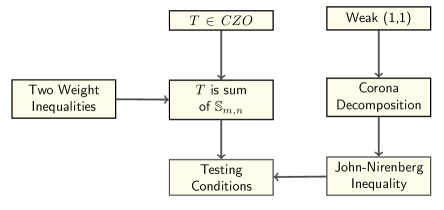
Figure 1. Proof Strategy

2. Haar Shift Operators

In this section, we introduce fundamental dyadic approximations of Calderón–Zygmund operators, the Haar shifts, and make a detailed reduction of the Main Theorem 1.3 to a similar statement, Theorem 2.14, in this dyadic model.

Definition 2.1.

A dyadic grid is a collection $\mathcal{D}$ of cubes so that for each $Q$ we have that

1. The set of cubes $\{Q^{\prime}\in\mathcal{D}\;:\;\lvert Q^{\prime}\rvert=\lvert Q\rvert\}$ partition $\mathbb{R}^{d}$, ignoring overlapping boundaries of cubes.

2. $Q$ is a union of cubes in a collection $\textup{Child}(Q)\subset\mathcal{D}$, called the children of $Q$. There are $2^{d}$ children of $Q$, each of volume $\lvert Q^{\prime}\rvert=2^{-d}\lvert Q\rvert$.

We refer to any subset of a dyadic grid as simply a grid.

The standard choice for $\mathcal{D}$ consists of the cubes $2^{k}\prod_{s=1}^{d}[n_{s},n_{s}+1)$ for $k,n_{1},\dotsc,n_{d}\in\mathbb{Z}$. But, the main result of this section, Theorem 2.7, depends upon a random family of dyadic grids.

In higher dimensions, we mention that the martingale differences are finite rank projections, but there is no canonical choice of the Haar functions in this case. We make the following definition.

Definition 2.2.

Let $Q$ be a dyadic cube, a generalized Haar function associated to $Q$, $h_{Q}$, is a linear combination of the indicator functions $\displaystyle\left\{\mathbf{1}_{Q}\right\}\cup\left\{\mathbf{1}_{Q^{\prime}}:Q^{\prime}\text{ is a child of }Q\right\}$,

$$h_{Q}=\sum_{Q^{\prime}\in\textup{Child}(Q)}c_{Q^{\prime}}\mathbf{1}_{Q^{\prime}}$$

We say $h_{Q}$ is a Haar function if in addition $\int h_{Q}=0$, that is, a Haar function is orthogonal to constants on its support.

Definition 2.3.

For integers $(m,n)\in\mathbb{Z}_{+}^{2}$, we say that a linear operator $\mathbb{S}$ is a (generalized) Haar shift operator of complexity type $(m,n)$ if

(2.4) $$\mathbb{S}f(x)=\sum_{Q\in\mathcal{D}}\mathbb{S}_{Q}f(x)=\sum_{Q\in\mathcal{D}}\quad\sideset{}{{}^{(m,n)}}{\sum}_{\begin{subarray}{c}Q^{\prime},R^{\prime}\in\mathcal{D}\\ Q^{\prime},R^{\prime}\subset Q\end{subarray}}\frac{\langle f,h^{Q^{\prime}}_{R^{\prime}}\rangle}{\lvert Q\rvert}k^{R^{\prime}}_{Q^{\prime}}(x)$$

where here and throughout $\ell(Q)=\lvert Q\rvert^{1/d}$, and

• in the second sum, the superscript ^(m,n) on the sum means that in addition we require $\ell(Q^{\prime})=2^{-m}\ell(Q)$ and $\ell(R^{\prime})=2^{-n}\ell(Q)$, and

• the function $h^{Q^{\prime}}_{R^{\prime}}$ is a (generalized) Haar function on $R^{\prime}$, and $k^{R^{\prime}}_{Q^{\prime}}$ is one on $Q^{\prime}$, with the normalization that

  (2.5) $$\lVert h^{Q^{\prime}}_{R^{\prime}}\rVert_{\infty}\leq 1,\qquad\lVert k^{R^{\prime}}_{Q^{\prime}}\rVert_{\infty}\leq 1\,.$$

Here, and throughout the paper, $\ell(Q)=\lvert Q\rvert^{1/d}$ is the side length of the cube $Q$. We say that the complexity of $\mathbb{S}$ is $\kappa:=\max(m,n,1)$.

A generalized Haar shift thus has the form

$$\mathbb{S}f\left(x\right)=\sum_{Q\in\mathcal{D}}\frac{1}{\left|Q\right|}\int_{Q}s_{Q}\left(x,y\right)f\left(y\right)dy=\int_{\mathbb{R}^{n}}K_{\mathbb{S}}\left(x,y\right)f\left(y\right)dy,$$

where $s_{Q}$, the kernel of the component $\mathbb{S}_{Q}$, is supported on $Q\times Q$ and $\left\|s_{Q}\right\|_{\infty}\leq 1$. It is easy to check that

$$|K_{\mathbb{S}}(x,y)|\lesssim\frac{1}{|x-y|^{d}}.$$

The Haar shifts are automatically bounded on $L^{2}$ with $\|\mathbb{S}f\|_{L^{2}}\leq\|f\|_{L^{2}}$. This follows from the imposed normalizations and simple orthogonality considerations. It is clear that all restricted shifts $\mathbb{S}_{\mathcal{Q}}f=\sum_{Q\in\mathcal{Q}}\mathbb{S}_{Q}f$ are also Haar shifts, and hence uniformly bounded on $L^{2}$ for any $\mathcal{Q}\subset\mathcal{D}$. We will extensively exploit these restricted shifts in the argument.

The generalized Haar shifts are only of relevance to us in two particular special cases of complexity type $(0,0)$, where $\mathbb{S}_{Q}f=|Q|^{-1}\langle f,h_{Q}^{Q}\rangle k_{Q}^{Q}=|Q|^{-1}\langle f,h_{Q}\rangle k_{Q}$. These are the paraproduct, where $h_{Q}=\mathbf{1}_{Q}$ and $k_{Q}$ is a Haar function for all $Q$, and the dual paraproduct, where $h_{Q}$ is a Haar function and $k_{Q}=\mathbf{1}_{Q}$ for all $Q$.

It is well-known that the (normalized) $L^{2}$ boundedness of a (dual) paraproduct is equivalent to the Carleson condition

$$\sum_{Q\subset R}\|k_{Q}\|_{L^{2}}^{2}\leq|R|\qquad\Big{(}\sum_{Q\subset R}\|h_{Q}\|_{L^{2}}^{2}\leq|R|\Big{)}\qquad\forall R\in\mathcal{D}.$$

These conditions are also uniformly inherited by all restricted (dual) paraproducts $\mathbb{S}_{\mathcal{Q}}$.

Note that for both Haar shifts and the paraproduct, we have

$$\int\mathbb{S}_{Q}f=0\qquad\forall Q\in\mathcal{D},$$

an important cancellation property in some of the later arguments. This is not the case for the dual paraproduct, for which a separate case study is needed at some points.

Remark 2.6.

Let

$$\delta\left(x,y\right)=\min\left\{\ell\left(Q\right):x,y\in Q\in\mathcal{D}\right\}$$

be the dyadic distance between $x$ and $y$. The kernel $K_{\mathbb{S}}\left(x,y\right)$ of $\mathbb{S}$ satisfies the size and smoothness conditions for a dyadic Calderón–Zygmund kernel:

$$\left|K_{\mathbb{S}}\left(x,y\right)\right| \leq \frac{2}{\delta\left(x,y\right)^{d}},$$

$$\left|K_{\mathbb{S}}\left(x,y\right)-K_{\mathbb{S}}\left(x^{\prime},y\right)\right| = 0\text{ if }\frac{\delta\left(x,x^{\prime}\right)}{\delta\left(x,y\right)}<\frac{1}{2^{m}},$$

$$\left|K_{\mathbb{S}}\left(x,y\right)-K_{\mathbb{S}}\left(x,y^{\prime}\right)\right| = 0\text{ if }\frac{\delta\left(y,y^{\prime}\right)}{\delta\left(x,y\right)}<\frac{1}{2^{n}}.$$

This is a more general dyadic kernel condition than one studied in [MR1934198], called perfect dyadic, which corresponds to $m=n=0$ in our framework.

The relevance of Haar shifts to Classical Analysis is explained by the following Theorem, one of the main results of [1010.0755] (see [1010.0755]*Theorem 4.1; also [1007.4330]*Theorem 4.2). This Theorem must be formulated in terms of a random dyadic grids. But the nature of this construction of grids is immaterial to the arguments of this paper, and refer the reader to these references for proofs, history, and further discussion of this result.

Theorem 2.7.

There is a collection of random dyadic grids $\{\mathcal{D}_{\beta}\;:\;\beta\in\boldsymbol{\beta}\}$, with expectation operator $\mathbb{E}_{\beta}$, for which the following holds. Let $T$ be a Calderón-Zygmund Operator $T$ with smoothness parameter $\delta$. Then, for all bounded and compactly supported functions $f$ and $g$, we can write

(2.8) $$\langle Tf,g\rangle=C\mathbb{E}_{\beta}\sum_{(m,n)\in\mathbb{Z}_{+}^{2}}2^{-(m+n)\delta/2}\langle\mathbb{S}_{m,n}^{\beta}f,g\rangle$$

where

• $\mathbb{S}_{m,n}^{\beta}$ is a Haar shift of complexity type $(m,n)$ for all $(m,n)\in\mathbb{Z}_{+}^{2}\setminus\{(0,0)\}$;

• $\mathbb{S}_{0,0}^{\beta}$ is the sum of a Haar shift of type $(0,0)$, a paraproduct, and a dual paraproduct;

• the constant $C$ is a function of $T$, and of the smoothness parameter $\delta$.

In particular we have the uniform estimate $\|\mathbb{S}_{m,n}^{\beta}\|_{L^{2}\to L^{2}}\leq 1$.

We define the maximal truncations of a Haar Shift as follows.

Definition 2.9.

Suppose that $\mathbb{S}$ is a generalized Haar shift. Define the associated maximal truncations by

$$\mathbb{S}_{\natural}f(x)\equiv\sup_{0<\epsilon\leq\upsilon<\infty}\lvert\mathbb{S}_{\epsilon,\upsilon}f(x)\rvert\,,$$

(2.10) $$\mathbb{S}_{\epsilon,\upsilon}f\equiv\sum_{Q\in\mathcal{D}:\ \epsilon\leq\ell(Q)\leq\upsilon}\mathbb{S}_{Q}f(x).$$

Proposition 2.11.

We have the pointwise bound

$$T_{\natural}f(x)\leq C(T)\mathbb{E}_{\beta}\sum_{(m,n)\in\mathbb{Z}^{2}_{+}}2^{-(m+n)\delta/2}(\mathbb{S}^{\beta}_{m,n})_{\natural}f(x)+C(T)Mf(x),$$

where $M$ is the Hardy-Littlewood maximal operator.

Proof.

Theorem 2.7 says that

$$\langle Tf,g\rangle=C(T)\mathbb{E}_{\beta}\sum_{(m,n)\in\mathbb{Z}^{2}_{+}}2^{-(m+n)\delta/2}\langle\mathbb{S}^{\beta}_{m,n}f,g\rangle$$

for bounded and compactly supported functions $f$ and $g$. By choosing

$$f=\frac{\mathbf{1}_{B(y,\epsilon)}}{|B(y,\epsilon)|}\qquad\textrm{and}\qquad g=\frac{\mathbf{1}_{B(x,\epsilon)}}{|B(x,\epsilon)|}$$

and taking the limit as $\epsilon\to 0$, dominated convergence implies the pointwise identity

(2.12) $$K(x,y)=C(T)\mathbb{E}_{\beta}\sum_{(m,n)\in\mathbb{Z}^{2}_{+}}2^{-(m+n)\delta/2}\sum_{Q\in\mathcal{D}^{\beta}}\frac{s^{m,n}_{Q}(x,y)}{|Q|}.$$

For $\epsilon>0$, this implies by Fubini’s theorem that

$$\int_{|x-y|\geq\epsilon} K(x,y)f(y)\,dy$$

$$=C(T)\mathbb{E}_{\beta}\sum_{(m,n)\in\mathbb{Z}^{2}_{+}}2^{-(m+n)\delta/2}\sum_{Q\in\mathcal{D}^{\beta}}\frac{1}{|Q|}\int_{B(x,\epsilon)^{c}}s_{Q}^{m,n}(x,y)f(y)\,dy.$$

Let us then decompose

$$\sum_{Q\in\mathcal{D}^{\beta}}\frac{1}{|Q|}\int_{B(x,\epsilon)^{c}}s_{Q}^{m,n}(x,y)f(y)\,dy =\mathop{\sum_{Q\in\mathcal{D}^{\beta}}}_{\ell(Q)>\epsilon^{\prime}}\frac{1}{|Q|}\int s_{Q}^{m,n}(x,y)f(y)\,dy$$

$$\quad-\mathop{\sum_{Q\in\mathcal{D}^{\beta}}}_{\ell(Q)>\epsilon^{\prime}}\frac{1}{|Q|}\int_{B(x,\epsilon)}s_{Q}^{m,n}(x,y)f(y)\,dy$$

$$\quad+\mathop{\sum_{Q\in\mathcal{D}^{\beta}}}_{\ell(Q)\leq\epsilon^{\prime}}\frac{1}{|Q|}\int_{B(x,\epsilon)^{c}}s_{Q}^{m,n}(x,y)f(y)\,dy$$

$$=I+I\!I+I\!I\!I,$$

where $\epsilon^{\prime}=\epsilon/(2\sqrt{d})$. By definition, there holds $|I|\leq(\mathbb{S}^{\beta}_{m,n})_{\natural}f(x)$. There also holds

$$|I\!I|\leq\sum_{k:\,2^{k}>\epsilon^{\prime}}2^{-kd}\int_{B(x,\epsilon)}|f|\lesssim\epsilon^{d}\Big{(}\sum_{k:\,2^{k}>\epsilon^{\prime}}2^{-kd}\Big{)}Mf(x)\lesssim Mf(x).$$

Furthermore, we actually have $I\!I\!I=0$, since there we must have $|x-y|\leq d(Q)=\sqrt{d}\ell(Q)\leq\sqrt{d}\epsilon^{\prime}=\epsilon/2<\epsilon$. We have thus shown that

$$T_{\epsilon}f(x)\leq C(T)\mathbb{E}_{\beta}\sum_{(m,n)\in\mathbb{Z}^{2}_{+}}2^{-(m+n)\delta/2}(\mathbb{S}^{\beta}_{m,n})_{\natural}f(x)+C(T)Mf(x)$$

for every $\epsilon>0$, and from this the proposition follows. ∎

Proposition 2.11 and Buckley’s [MR1124164] sharp weighted bounds for the maximal operator,

(2.13) $$\|Mf\|_{L^{p,\infty}(w)}\lesssim\|w\|_{A_{p}}^{1/p}\|f\|_{L^{p}(w)},\qquad\|Mf\|_{L^{p}(w)}\lesssim\|w\|_{A_{p}}^{1/(p-1)}\|f\|_{L^{p}(w)},$$

reduce the proof of the Main Theorem 1.3 to the verification of the following dyadic variant, a task which occupies the rest of this paper.

Theorem 2.14.

Let $\mathbb{S}$ be a Haar shift operator with complexity $\kappa$, a paraproduct, or a dual paraproduct. For $1<p<\infty$ and $w\in A_{p}$, we then have the estimates

(2.15) $$\lVert\mathbb{S}_{\natural}f\rVert_{L^{p,\infty}(w)} \lesssim\kappa\lVert w\rVert_{A_{p}}\lVert f\rVert_{L^{p}(w)}\,,$$

(2.16) $$\lVert\mathbb{S}_{\natural}f\rVert_{L^{p}(w)} \lesssim\kappa\lVert w\rVert_{A_{p}}^{\max\{1,(p-1)^{-1}\}}\lVert f\rVert_{L^{p}(w)}$$

Indeed, any polynomial dependence on the complexity parameter $\kappa$ would suffice for Theorem 1.3, but a careful tracing of the constants will even provide the linear dependence, as stated. Even for the untruncated shifts $\mathbb{S}$ in $L^{2}(w)$, this improves on the quadratic in $\kappa$ bound established in [1010.0755] (but we are not aware of an application where this precision in the dependence on $\kappa$ would be of importance).

The dependence on $\kappa$ and the weight constant $\|w\|_{A_{p}}$ arises from the following points of the proof below: First, we establish two-weight inequalities of the form

(2.17) $$\lVert\mathbb{S}_{\natural}(f\sigma)\rVert_{L^{p,\infty}(w)} \lesssim\left\{\kappa\mathfrak{M}_{p,\operatorname{weak}}+\mathfrak{T}_{p}\right\}\lVert f\rVert_{L^{p}(\sigma)},$$

(2.18) $$\lVert\mathbb{S}_{\natural}(f\sigma)\rVert_{L^{p}(w)} \lesssim\left\{\kappa\mathfrak{M}_{p}+\mathfrak{T}_{p}+\mathfrak{N}_{p}\right\}\lVert f\rVert_{L^{p}(\sigma)},$$

where $\mathfrak{M}_{p,\operatorname{weak}}$ and $\mathfrak{M}_{p}$ are the best constants from certain maximal inequalities, while $\mathfrak{T}_{p}$ and $\mathfrak{N}_{p}$ are the best constants from appropriate testing conditions for the operator $\mathbb{S}_{\natural}$. Here, $w$ and $\sigma$ are allowed to be an arbitrary pair of weights, with no relation to each other.

Second, we specialize to the one-weight situation with $\sigma=w^{1-p^{\prime}}$, using a well-known dual-weight formulation of the bounds to be proven, (2.15) and (2.16). We need to estimate the above four constants in this situation. The maximal constants are independent of $\mathbb{S}_{\natural}$ and thus of $\kappa$, and they satisfy $\mathfrak{M}_{p,\operatorname{weak}}\lesssim\|w\|_{A_{p}}^{1/p}$ and $\mathfrak{M}_{p}\lesssim\|w\|_{A_{p}}^{1/(p-1)}$ by the sharp maximal function inequalities of Buckley (2.13). For the two testing constants related to $\mathbb{S}_{\natural}$, we obtain the linear in $\kappa$ bounds

$$\mathfrak{T}_{p}\lesssim\kappa\|w\|_{A_{p}},\qquad\mathfrak{N}_{p}\lesssim\kappa\|w\|_{A_{p}}^{1/(p-1)}.$$

This dependence comes from the fact that the proof of the John–Nirenberg style estimates of (10.14) requires separating the scales of $\mathbb{S}$ by dividing it into $\kappa+1$ parts, each of which contains nonzero components $\mathbb{S}_{Q}$ only for a fixed value of $\log_{2}\ell(Q)\mod(\kappa+1)$. For these separated parts of $\mathbb{S}$, our bounds will be independent of $\kappa$, and it remains to sum up.

3. Linearizing Maximal Operators

A fundamental tool is derived from (the usual) general maximal function estimates that hold for any measure. In particular, for weight $w$ we define

(3.1) $$M_{w}f(x) \equiv\sup_{Q\in\mathcal{D}}\mathbf{1}_{Q}(x)\mathbb{E}_{Q}^{w}\lvert f\rvert\,,$$

(3.2) $$\mathbb{E}_{Q}^{w}f \equiv w(Q)^{-1}\int_{Q}f\,w(dx)\,.$$

The notation $\mathbb{E}_{Q}f$ means that the implied measure is Lebesgue. It is a basic fact, proved by exactly the same methods that prove the non-weighted inequality, that we have the estimate below, which will be used repeatedly.

Theorem 3.3.

We have the inequalities

(3.4) $$\left\|M_{w}f\right\|_{L^{p}(w)}\lesssim\left\|f\right\|_{L^{p}(w)}\,,\qquad 1<p<\infty\,.$$

We use the method of linearizing maximal operators. This is familiar in the context of the maximal function, and we make a comment about it here. Let $\{E(Q)\;:\;Q\in\mathcal{D}\}$ be any selection of measurable disjoint sets $E(Q)\subset Q$ indexed by the dyadic cubes. Define a corresponding linear operator $N$ by

(3.5) $$N\phi\equiv\sum_{Q\in\mathcal{D}}\mathbf{1}_{E(Q)}\mathbb{E}_{Q}^{w}f\,.$$

Then, the universal Maximal function bound (3.4) is equivalent to the bound $\left\|Nf\right\|_{L^{p}(w)}\lesssim\left\|f\right\|_{L^{p}(w)}$ with implied constant independent of $w$ and the sets $\{E(Q)\;:\;Q\in\mathcal{D}\}$. This estimate will be used repeatedly below.

There is a related way to linearize $\mathbb{S}_{\natural}$, which deserves careful comment as we would like, at different points, to treat $\mathbb{S}_{\natural}$ as a linear operator. While it is not a linear operator, $\mathbb{S}_{\natural}$ is a pointwise supremum of the linear truncation operators $\mathbb{S}_{\varepsilon,\upsilon}$, and as such, the supremum can be linearized with measurable selection of the truncation parameters.

Definition 3.6.

We say that $\mathbb{L}$ is a linearization of $\mathbb{S}_{\natural}$ if there are measurable functions $\epsilon(x),\upsilon(x)\in(0,\infty)$ and $\vartheta(x)\in[0,2\pi)$ such that, using (2.10), we have

(3.7) $$\mathbb{L}f(x)=e^{i\vartheta(x)}\mathbb{S}_{\epsilon(x),\upsilon(x)}f(x)\geq 0,\qquad x\in\mathbb{R}^{d}.$$

Note that the requirement $\mathbb{L}f(x)\geq 0$ defines $\vartheta(x)$ everywhere except when $\mathbb{S}_{\epsilon(x),\upsilon(x)}f(x)=0$. Also, for fixed $f$ we can always choose a linearization $L$ so that $\mathbb{S}_{\natural}f(x)\leq 2\mathbb{L}f(x)$ for all $x$.

A key advantage of $\mathbb{L}$ is that it is a linear operator, and as such it has an adjoint, given by the formal expressions

(3.8) $$\begin{split}\mathbb{L}^{*}\nu(y)&=\sum_{Q\in\mathcal{D}}\mathbb{S}_{Q}^{*}(\mathbf{1}_{\{\epsilon(\cdot)\leq\ell(Q)\leq\upsilon(\cdot)\}}e^{i\vartheta(\cdot)}\nu)(y)\\ &=\sum_{Q\in\mathcal{D}}\frac{1}{|Q|}\int_{Q}s_{Q}(x,y)\mathbf{1}_{\{\epsilon(x)\leq\ell(Q)\leq\upsilon(x)\}}e^{i\vartheta(x)}\nu(dx).\end{split}$$

The following ‘smoothness’ property of $\mathbb{L}^{\ast}$ is an important observation in the proof of our two weight estimates.

Lemma 3.9.

Suppose that for a measure $\nu$ and cube $Q_{0}$ we have $\lvert\nu\rvert(Q_{0})=0$. Suppose that $\mathbb{S}$ has complexity type $\left(m,n\right)$. Then $\mathbb{L}^{\ast}\nu(\cdot)$ is constant on subcubes $Q^{\prime}\subset Q_{0}$ with $\ell(Q^{\prime})\leq 2^{-n}\ell(Q_{0})$.

Proof.

For $y\in Q_{0}$, the sum in (3.8) defining the adjoint operator becomes

$$\mathbb{L}^{*}\nu(y)=\sum_{Q\in\mathcal{D}:\ Q\supsetneq Q_{0}}\frac{1}{|Q|}\int_{Q}s_{Q}(x,y)\mathbf{1}_{\{\epsilon(x)\leq\ell(Q)\leq\upsilon(x)\}}e^{i\vartheta(x)}\nu(dx).$$

As a function of $y$, the kernel $s_{Q}(x,y)$ is constant on the subcubes of $R^{\prime}\subset Q$ with $\ell(R^{\prime})\leq 2^{-n-1}\ell(Q)$. Thus for $Q\supsetneq Q_{0}$, it is in particular constant on the subcubes $Q^{\prime}\subset Q_{0}$ with $\ell(Q^{\prime})\leq 2^{-n}\ell(Q_{0})$. ∎

4. The Two Weight Estimates

We are interested in tracking complexity dependence in two weight inequalities for Haar Shift Operators, as defined in §2. We study the maximal truncations of such operators, and obtain sufficient conditions for the weak and strong type $(p,p)$ two weight inequalities for such operators. Our main results are Theorem 4.6 for the weak type result, and Theorem 4.11 for the strong type result. These Theorems give sufficient conditions in terms of the Maximal Function, and certain testing conditions. Of particular import here is that these sufficient conditions are efficient in terms of the complexity of the Haar Shift operator.

Our primary focus concerns extensions of the dyadic $T1$ Theorem to the two weight setting. These considerations are motivated in part by a well developed theory of two weight estimates for positive operators. These Theorems have formulations strikingly similar to the $T1$ Theorem, which theory encompasses the Theorems due to one of us concerning two weight, both strong and weak type, for the maximal operator [MR676801] and fractional integral operators [MR719674], [MR930072]. There is also the bilinear embedding inequality of Nazarov-Treil-Volberg [MR1685781]. We refer the reader to [0911.3437] for a discussion of these results.

There is a beautiful result of Nazarov-Treil-Volberg [NTV2], a two-weight version of the $T1$ theorem. A subcase of their result was proved for Haar Shifts, with an effective bound on complexity in [1010.0755]*Theorem 3.4.

Theorem 4.1.

Let $\mathbb{S}$ be a Haar Shift operator of complexity $\kappa$, as in Definition 2.3. Let $\sigma,w$ be two positive locally finite measures. We have the inequality

(4.2) $$\lVert\mathbb{S}(f\sigma)\rVert_{L^{2}(w)}\lesssim\kappa\{\mathfrak{S}+\mathfrak{S}^{\ast}\}+\kappa^{2}\lVert w,\sigma\rVert_{A_{2}}^{{1/2}}$$

where the three quantities above are defined by

(4.3) $$\lVert w,\sigma\rVert_{A_{2}} :=\sup_{Q}\frac{w(Q)}{\lvert Q\rvert}\frac{\sigma(Q)}{\lvert Q\rvert}$$

(4.4) $$\mathfrak{S} :=\sup_{Q}\sigma(Q)^{-1/2}\lVert\mathbf{1}_{Q}\mathbb{S}(\sigma\mathbf{1}_{Q})\rVert_{L^{2}(w)}\,.$$

(4.5) $$\mathfrak{S}^{\ast} :=\sup_{Q}w(Q)^{-1/2}\lVert\mathbf{1}_{Q}\mathbb{S}^{\ast}(w\mathbf{1}_{Q})\rVert_{L^{2}(\sigma)}\,.$$

The first of the three conditions is the two weight $A_{2}$ condition; the remaining two are the testing conditions. The proof is fundamentally restricted to the case of $p=2$, nor does it address maximal truncations. We will consider the case of $1<p<\infty$ and obtain sufficient conditions for the two weight inequalities for the maximal operator $\mathbb{S}_{\natural}$. First we give the weak type result. Below, $M$ denotes the maximal function.

Theorem 4.6.

Let $\mathbb{S}$ be a generalized Haar shift of complexity $\kappa$ as in Definition 2.3. Then we have the weak type inequality

(4.7) $$\left\|\mathbb{S}_{\natural}(f\sigma)\right\|_{L^{p,\infty}(w)}\lesssim\left(\kappa\mathfrak{M}_{p,\textup{weak}}+\mathfrak{T}_{p}\right)\left\|f\right\|_{L^{p}(\sigma)}\,,$$

where the constants $\mathfrak{M}_{p,\textup{weak}}$ and $\mathfrak{T}_{p}$ are the best such in the following inequalities

(4.8) $$\left\|{M}(f\sigma)\right\|_{L^{p,\infty}(w)}\leq\mathfrak{M}_{p,\textup{weak}}\left\|f\right\|_{L^{p}(\sigma)}\,,$$

(4.9) $$\int_{Q}\mathbb{S}_{\natural}(\sigma f\mathbf{1}_{Q})\,\;w(dx)\leq\mathfrak{T}_{p}\left\|f\right\|_{L^{p}(\sigma)}w(Q)^{1/p^{\prime}}.$$

The point of this Theorem is that to check the weak-type inequality for $\mathbb{S}_{\natural}$, it suffices to check the weak-type inequality for the simpler maximal operator $M$, and to check only particular instances of the weak-type inequality for $\mathbb{S}_{\natural}$. It is also important that the complexity $\kappa$ appears with polynomial growth.

The dual testing condition (4.9) looks rather complicated, with the appearance of $f\in L^{p}(\sigma)$ in it. However, $\mathbb{S}_{\natural}$ appears to just the first power, and it is a close relative of (4.5). Indeed, (4.9) has a more convincing formulation in the linearizations. It is equivalent to the dual testing condition

(4.10) $$\left\|\mathbf{1}_{Q}\mathbb{L}^{\ast}(\mathbf{1}_{Q}gw)\right\|_{L^{p^{\prime}}(\sigma)}\leq\mathfrak{T}_{p}w(Q)^{1/p^{\prime}}\left\|g\right\|_{\infty},$$

This holds uniformly over all choices of linearizations, which fact is referred to repeatedly below. Inequality (4.10) reflects the fact that the dual of a weak type inequality is a restricted strong type inequality.

Our strong type result will require duals $\mathbb{L}^{\ast}$ of linearizations $\mathbb{L}$ of $\mathbb{S}_{\natural}$ in order to state the nonstandard testing condition in (4.14). These were defined in Section 3 above.

Theorem 4.11.

Let $\mathbb{S}$ be a generalized Haar shift of complexity $\kappa$ as in Definition 2.3. We have the following quantitative estimate:

(4.12) $$\lVert\mathbb{S}_{\natural}(f\sigma)\rVert_{L^{p}(w)}\lesssim\left\{\kappa\mathfrak{M}_{p}+\mathfrak{T}_{p}+\mathfrak{N}_{p}\right\}\lVert f\rVert_{L^{p}(\sigma)}\,,$$

where $\mathfrak{T}_{p}$ is defined in (4.9), and the numbers $\mathfrak{M}_{p}$ and $\mathfrak{N}_{p}$ are defined in

(4.13) $$\left\|{M}(f\sigma)\right\|_{L^{p}(w)}\leq\mathfrak{M}_{p}\left\|f\right\|_{L^{p}(\sigma)},$$

(4.14) $$\mathfrak{N}_{p}^{p}\equiv\sup_{\left\|\varphi\right\|_{\infty}\leq 1}\sup_{Q_{0}}\frac{1}{\sigma(Q_{0})}\int_{Q_{0}}\sup_{Q\subset Q_{0}}\mathbf{1}_{Q}\left(\frac{1}{w(Q)}\int_{Q}\left|\mathbb{L}^{\ast}(\mathbf{1}_{Q}\varphi w)(y)\right|\sigma(dy)\right)^{p}w(dx).$$

As a new kind of complication compared to the weak-type case, we have the nonstandard testing condition (4.14). Its primary difficulty is the appearance of $\left|\mathbb{L}^{\ast}\right|$ integrated over $Q$ with respect to $\sigma$, but then divided by $w(Q)$ rather than the usual $\sigma(Q)$. Also there is an additional supremum, with the argument of $\mathbb{L}^{\ast}$ dependent upon the cube $Q$ over which we are taking the supremum.

The method of proof is an extension of that of Sawyer’s approach to the two weight fractional integrals [MR930072], but see also [0911.3437]. This argument follows the outlines of the proof in [0807.0246], which proves variants of Theorem 4.6 and Theorem 4.11 for smooth Calderón-Zygmund operators. The current arguments are, naturally, much easier while retaining the essential ideas and techniques of [0807.0246]. (The reader can also compare the arguments of this paper to those of [0911.3437].)

Let us give a guide to the next few sections of this paper, which are concerned with the proof of the above two-weight results.

§5:

Collects facts central to the proofs, maximal functions, linearizations of maximal functions, Whitney decompositions, and an important maximum principle.

§6:

The weak-type result Theorem 4.6 is proved.

§7:

Sufficient conditions for the strong type result are stated; the classical part of the proof of the strong type result Theorem 4.11 is begun.

§8:

This section contains the core of the proof of Theorem 4.11.

5. Generalities of the Proof

5.1. Whitney Decompositions

We make general remarks about the sets

(5.1) $$\Omega_{k}=\{\mathbb{S}_{\natural}(f\sigma)>2^{k}\}$$

where $f$ is a finite linear combination of indicators of dyadic cubes. For points $x$ sufficiently far away from the support of $f$, we will have that $\mathbb{S}_{\natural}(f\sigma)$ is dominated by the maximal function $M(f\sigma)$. Hence, the sets $\Omega_{k}$ will be open with compact closure.

Let $Q^{(1)}$ denote the dyadic parent of $Q$, and inductively define $Q^{(j+1)}=(Q^{(j)})^{(1)}$. For a nonnegative integer $\zeta$, let $\mathcal{Q}_{k}$ be the collection of maximal dyadic cubes $Q$ such that $Q^{(\zeta)}\subset\Omega_{k}$. Then

(5.2) $$\Omega_{k}=\dot{\bigcup_{Q\in\mathcal{Q}_{k}}}Q\ \ \ \ \ \text{{(disjoint cover),}}$$

(5.3) $$Q^{(\zeta)}\subset\Omega_{k}\,,\ Q^{(\zeta+1)}\cap\Omega_{k}^{c}\neq\emptyset\ \ \ \ \ \text{{(Whitney condition,)}}$$

(5.4) $$Q\in\mathcal{Q}_{k}\,,\ Q^{\prime}\in\mathcal{Q}_{l}\,,\ Q\subsetneqq Q^{\prime}\quad\textup{implies}\quad k>l\ \ \ \ \ \text{{(nested property).}}$$

Remark 5.5.

In the proof of the weak type theorem we will take $\zeta=0$. In the proof of the strong type theorem we will take $\zeta=n+1\leq\kappa+1$, when the shift under consideration has complexity type $(m,n)$.

5.2. Maximum Principle

A fundamental tool is the use of what we term here as a ‘maximum principle’ (we could also use the term ‘good-$\lambda$ technique’): Subject to the assumption that the maximal function $M$ is of small size, we will be able to see that the maximal truncations are large due to the restriction of the function to a local cube. This leads to an essential ‘localization’ of the singular integrals.

Theorem 5.6 (Maximum Principle).

Let $\mathbb{S}$ be a generalized Haar shift of complexity type $\left(m,n\right)$. For any cube $Q\in\mathcal{Q}_{k}$ as in the Whitney decomposition of $\Omega_{k}$ in (5.1) above with parameter $\zeta$, we have the pointwise inequality

(5.7) $$\begin{split}\mathbb{S}_{\natural}\left(f\sigma\right)\left(x\right)&\leq\sup_{\epsilon\leq\upsilon\leq\ell(Q)}|\mathbb{S}_{\epsilon,\upsilon}(f\sigma)(x)|+2^{k}+(\zeta+n+1)M(f\sigma)(x)\\ &\leq\mathbb{S}_{\natural}(f1_{Q}\sigma)(x)+2^{k}+(\zeta+n+1)M(f\sigma)(x).\end{split}$$

There is a corresponding Maximum Principle in Section 3.3 of [0911.3437], which is very effective in the positive operator case. As our operators are not positive, and as we are ultimately only interested in the one weight situation, we have the maximal function $M$ on the right in (5.7).

Proof.

Note that the second inequality of the claim is obvious, since $\mathbb{S}_{\epsilon,\upsilon}(f\sigma)(x)=\mathbb{S}_{\epsilon,\upsilon}(f1_{Q}\sigma)(x)$ when $x\in Q$ and $\epsilon\leq\upsilon\leq\ell(Q)$. We prove the first inequality.

Let $x\in Q\in\mathcal{Q}_{k}$, and let $r:=(\zeta+1)+(n+1)$. Then

$$\begin{split}\mathbb{S}_{\epsilon,\upsilon}(f\sigma)(x)&=\sum_{I:\epsilon\leq\ell(I)\leq\upsilon}\mathbb{S}_{I}(f\sigma)(x)\\ &=\Big{(}\sum_{\begin{subarray}{c}I:\epsilon\leq\ell(I)\leq\upsilon\\ \ell(I)\leq\ell(Q)\end{subarray}}+\sum_{\begin{subarray}{c}I:\epsilon\leq\ell(I)\leq\upsilon\\ \ell(I)\geq 2^{r}\ell(Q)\end{subarray}}+\sum_{\begin{subarray}{c}I:\epsilon\leq\ell(I)\leq\upsilon\\ \ell(Q)<\ell(I)<2^{r}\ell(Q)\end{subarray}}\Big{)}\mathbb{S}_{I}(f\sigma)(x)\\ &=\mathbb{S}_{\epsilon,\min(\upsilon,\ell(Q))}(f\sigma)(x)+\mathbb{S}_{\max(\epsilon,2^{r}\ell(Q)),\upsilon}(f\sigma)(x)+\sum_{\begin{subarray}{c}I:\epsilon\leq\ell(I)\leq\upsilon\\ \ell(Q)<\ell(I)<2^{r}\ell(Q)\end{subarray}}\mathbb{S}_{I}(f\sigma)(x).\end{split}$$

The first term on the right is clearly dominated by $\sup_{\epsilon^{\prime}\leq\upsilon^{\prime}\leq\ell(Q)}|\mathbb{S}_{\epsilon^{\prime},\upsilon^{\prime}}(f\sigma)(x)|$. All $\mathbb{S}_{I}(f\sigma)$ participating in the second term have $\ell(I)\geq 2^{n+1}\ell(Q^{(\zeta+1)})$, so they are constant on $Q^{(\zeta+1)}$. Hence we may replace $x$ by some $\bar{x}\in Q^{(\zeta+1)}\setminus\Omega_{k}$ (which is nonempty by definition of $\mathcal{Q}_{k}$). So this second term is dominated by

$$\mathbb{S}_{\natural}(f\sigma)(\bar{x})\leq 2^{k}.$$

Finally, the last term contains at most $r-1=\zeta+n+1$ summands, each of which is dominated by $M(f\sigma)(x)$. ∎

6. Proof of the Weak-Type Inequality

We prove Theorem 4.6, stating that

$$\|\mathbb{S}_{\natural}(f\sigma)\|_{L^{p,\infty}(w)}\lesssim(\kappa\mathfrak{M}_{p,\textup{weak}}+\mathfrak{T}_{p})\|f\|_{L^{p}(\sigma)}.$$

To this end, we need to estimate the quantities

$$w(\mathbb{S}_{\natural}(f\sigma)>4\cdot 2^{k})\leq w(M(f\sigma)>\eta 2^{k})+w(\mathbb{S}_{\natural}(f\sigma)>4\cdot 2^{k},M(f\sigma)\leq\eta 2^{k}),$$

where the small parameter $\eta$ is to be chosen shortly. Since $\Omega_{k+2}\subset\Omega_{k}=\bigcup_{Q\in\mathcal{Q}_{k}}Q$, where we take the Whitney decomposition with parameter $\zeta=0$, we further have that

$$\begin{split}w(\mathbb{S}_{\natural}(f\sigma)&>4\cdot 2^{k},M(f\sigma)\leq\eta 2^{k})\\ &=\sum_{Q\in\mathcal{Q}_{k}}w(Q\cap\{\mathbb{S}_{\natural}(f\sigma)>4\cdot 2^{k},M(f\sigma)\leq\eta 2^{k}\})=:\sum_{Q\in\mathcal{Q}_{k}}w(E_{k}(Q)).\end{split}$$

On $E_{k}(Q)\subset Q$, the maximum principle gives that

$$\begin{split}4\cdot 2^{k}<\mathbb{S}_{\natural}(f\sigma)&\leq\mathbb{S}_{\natural}(f1_{Q}\sigma)+2^{k}+(2n+3)M(f\sigma)\\ &\leq\mathbb{S}_{\natural}(f1_{Q}\sigma)+2^{k}+(2n+3)\eta 2^{k}\leq\mathbb{S}_{\natural}(f1_{Q}\sigma)+2\cdot 2^{k},\end{split}$$

provided that $\eta:=(2\kappa+3)^{-1}\leq(2n+3)^{-1}$. Thus

$$\mathbb{S}_{\natural}(f\sigma 1_{Q})>2^{k+1}\qquad\text{on }E_{k}(Q).$$

Putting these considerations together, we obtain (for another small parameter $\delta>0$)

$$\begin{split}(4\cdot 2^{k})^{p}&w(\mathbb{S}_{\natural}(f\sigma)>4\cdot 2^{k})\\ &\leq 4^{p}2^{kp}w(M(f\sigma)>\eta 2^{k})+2^{p}\sum_{Q\in\mathcal{Q}_{k}}2^{(k+1)p}w(E_{k}(Q))\\ &\leq 4^{p}\eta^{-p}\|M(f\sigma)\|_{L^{p,\infty}(w)}^{p}+4^{p}2^{kp}\sum_{\begin{subarray}{c}Q\in\mathcal{Q}_{k}\\ w(E_{k}(Q))<\delta w(Q)\end{subarray}}\delta w(Q)\\ &\qquad+2^{p}\sum_{\begin{subarray}{c}Q\in\mathcal{Q}_{k}\\ w(E_{k}(Q))\geq\delta w(Q)\end{subarray}}w(E_{k}(Q))\Big{(}\frac{1}{w(E_{k}(Q))}\int_{E_{k}(Q)}\mathbb{S}_{\natural}(f1_{Q}\sigma)w\Big{)}^{p}\\ &\leq 2^{p}\eta^{-p}\mathfrak{M}_{p,\textup{weak}}^{p}\|f\|_{L^{p}(\sigma)}^{p}+4^{p}\delta 2^{kp}w(\mathbb{S}_{\natural}(f\sigma)>2^{k})\\ &\qquad+2^{p}\sum_{Q\in\mathcal{Q}_{k}}\delta^{1-p}w(Q)^{1-p}\Big{(}\int_{Q}\mathbb{S}_{\natural}(f1_{Q}\sigma)w\Big{)}^{p}\end{split}$$

Picking a $k$ for which the left side is close to its supremum, and choosing $\delta=10^{-p}$, we can absorb the middle term on the right to the left side. Recalling the choice of $\eta$ and using the testing condition to the integrals in the last term, we obtain

$$\begin{split}\|\mathbb{S}_{\natural}(f\sigma)\|_{L^{p,\infty}(w)}^{p}&\lesssim\kappa^{p}\mathfrak{M}_{p,\textup{weak}}^{p}\|f\|_{L^{p}(\sigma)}+\sum_{Q\in\mathcal{Q}_{k}}w(Q)^{1-p}(\mathfrak{T}_{p}\|f1_{Q}\|_{L^{p}(\sigma)}w(Q)^{1/p^{\prime}}\big{)}^{p}\\ &=\kappa^{p}\mathfrak{M}_{p,\textup{weak}}^{p}\|f\|_{L^{p}(\sigma)}+\mathfrak{T}_{p}^{p}\sum_{Q\in\mathcal{Q}_{k}}\|f1_{Q}\|_{L^{p}(\sigma)}^{p}\\ &\leq\big{(}\kappa^{p}\mathfrak{M}_{p,\textup{weak}}^{p}+\mathfrak{T}_{p}^{p}\big{)}\|f\|_{L^{p}(\sigma)},\end{split}$$

by the disjointness of the $Q\in\mathcal{Q}_{k}$ in the last step.

7. First Steps in the Proof of the Strong Type Inequality

We start preparing for the proof of

$$\|\mathbb{S}_{\natural}(f\sigma)\|_{L^{p}(w)}\lesssim(\kappa\mathfrak{M}_{p}+\mathfrak{T}_{p}+\mathfrak{N}_{p})\|f\|_{L^{p}(\sigma)}.$$

In this section, we make an estimate of the form

$$\|\mathbb{S}_{\natural}(f\sigma)\|_{L^{p}(w)}\lesssim\kappa\mathfrak{M}_{p}\|f\|_{L^{p}(\sigma)}+\delta\|\mathbb{S}_{\natural}(f\sigma)\|_{L^{p}(w)}+\text{remainder},$$

where the second term with the small parameter $\delta$ may be absorbed to the right, and the ‘remainder’ will be controlled in terms on $(\mathfrak{T}_{p}+\mathfrak{N}_{p})\|f\|_{L^{p}(\sigma)}$ in the following section, which contains the core of the argument.

We begin with

$$\begin{split}\|\mathbb{S}_{\natural}(f\sigma)\|_{L^{p}(w)}^{p}&=\sum_{k\in\mathbb{Z}}\int_{\Omega_{k+1}\setminus\Omega_{k+2}}\mathbb{S}_{\natural}(f\sigma)^{p}w\\ &\leq 4^{p}\sum_{k\in\mathbb{Z}}2^{kp}w(\Omega_{k+1}\setminus\Omega_{k+2})\\ &=4^{p}\sum_{k\in\mathbb{Z}}2^{kp}\sum_{Q\in\mathcal{Q}_{k}}w(Q\cap(\Omega_{k+1}\setminus\Omega_{k+2}))\\ &=:4^{p}\sum_{k\in\mathbb{Z}}2^{kp}\sum_{Q\in\mathcal{Q}_{k}}w(F_{k}(Q)).\end{split}$$

Note that the sets $F_{k}(Q)$ are pairwise disjoint. We first employ a similar reduction as in the weak-type case:

(7.1) $$\begin{split}w(F_{k}(Q))&\leq w(F_{k}(Q)\cap\{M(f\sigma)>\eta 2^{k}\})+w(F_{k}(Q)\cap\{M(f\sigma)\leq\eta 2^{k}\})\\ &=:w(F_{k}(Q)\cap\{M(f\sigma)>\eta 2^{k}\})+w(E_{k}(Q)).\end{split}$$

Then

$$\begin{split}\sum_{k}2^{kp}\sum_{Q\in\mathcal{Q}_{k}}w(F_{k}(Q)\cap\{M(f\sigma)>\eta 2^{k}\})&\leq\eta^{-p}\sum_{k}\sum_{Q\in\mathcal{Q}_{k}}\int_{F_{k}(Q)}M(f\sigma)^{p}w\\ &\leq\eta^{-p}\|M(f\sigma)\|_{L^{p}(w)}^{p}\leq\eta^{-p}\mathfrak{M}_{p}^{p}\|f\|_{L^{p}(\sigma)}^{p}.\end{split}$$

We are left with

$$\begin{split}\sum_{k\in\mathbb{Z}}2^{kp}\sum_{Q\in\mathcal{Q}_{k}}w(E_{k}(Q))&\leq\sum_{k\in\mathbb{Z}}2^{kp}\sum_{\begin{subarray}{c}Q\in\mathcal{Q}_{k}\\ w(E_{k}(Q))<\delta w(Q)\end{subarray}}\delta w(Q)\\ &\qquad+\sum_{k\in\mathbb{Z}}2^{kp}\sum_{\begin{subarray}{c}Q\in\mathcal{Q}_{k}\\ w(E_{k}(Q))\geq\delta w(Q)\end{subarray}}w(E_{k}(Q)),\end{split}$$

and the first sum on the right is immediately dominated by

$$\delta\sum_{k\in\mathbb{Z}}2^{kp}w(\mathbb{S}_{\natural}(f\sigma)>2^{k})\lesssim\delta\|\mathbb{S}_{\natural}(f\sigma)\|_{L^{p}(w)}^{p},$$

so this term can be absorbed after a suitable small choice of $\delta>0$ depending only on $p$.

Now consider one of the remaining sets $E_{k}(Q)$ for $Q\in\mathcal{Q}_{k}$ and $w(E_{k}(Q))\geq\delta w(Q)$. By the maximum principle, we can choose a linearization $\mathbb{L}=e^{i\vartheta(x)}\mathbb{S}_{\epsilon(x),\upsilon(x)}$ of $\mathbb{S}_{\natural}$ with $\upsilon(x)\leq\ell(Q)$, so that, for $x\in E_{k}(Q)$,

$$\begin{split}4\cdot 2^{k}<\mathbb{S}_{\natural}(f\sigma)(x)&\leq 2\mathbb{L}(f\sigma)(x)+2^{k}+(\zeta+n+1)M(f\sigma)(x),\\ &\leq 2\mathbb{L}(f\sigma)(x)+2^{k}+(\zeta+n+1)\eta 2^{k}\\ &\leq 2\mathbb{L}(f\sigma)(x)+2\cdot 2^{k},\end{split}$$

by choosing

$$\eta:=(\zeta+n+1)^{-1}=(2n+2)^{-1}\gtrsim\kappa^{-1}.$$

Hence

$$\mathbb{L}(f\sigma)(x)\geq 2^{k}\qquad\text{on }E_{k}(Q).$$

Notice that, by the disjointness of the sets $E_{k}(Q)\subset F_{k}(Q)$, we can globally define one linearization $\mathbb{L}$, which fulfills this condition on all $E_{k}(Q)$.

Thus, for $w(E_{k}(Q))\geq\delta w(Q)$, we have

$$2^{kp}\leq\Big{(}\frac{1}{w(E_{k}(Q))}\int_{E_{k}(Q)}\mathbb{L}(f\sigma)w\Big{)}^{p}\leq\delta^{-p}\Big{(}\frac{1}{w(Q)}\int_{E_{k}(Q)}\mathbb{L}(f\sigma)w\Big{)}^{p},$$

where

$$\mathbb{L}=e^{i\vartheta(x)}\mathbb{S}_{\epsilon(x),\upsilon(x)},\qquad\upsilon(x)\leq\ell(Q)\text{ on }E_{k}(Q).$$

We have proven that (absorbing the term $\delta\|\mathbb{S}_{\natural}(f\sigma)\|_{L^{p}(\sigma)}^{p}$, and using $\eta^{-1}\lesssim\kappa$)

$$\|\mathbb{S}_{\natural}(f\sigma)\|_{L^{p}(\sigma)}^{p}\lesssim\kappa^{p}\mathfrak{M}_{p}^{p}\|f\|_{L^{p}(\sigma)}^{p}+\sum_{k\in\mathbb{Z}}\sum_{Q\in\mathcal{Q}_{k}}w(E_{k}(Q))\Big{(}\frac{1}{w(Q)}\int_{E_{k}(Q)}\mathbb{L}(f\sigma)w\Big{)}^{p}.$$

(The dependence on $\delta$ has been neglected, since this is in any case a function of $p$ only.)

8. Strong-type estimates: the core

We are left to prove that

(8.1) $$\sum_{k}\sum_{Q\in\mathcal{Q}_{k}}w(E_{k}(Q))\Big{|}\frac{1}{w(Q)}\int_{E_{k}(Q)}\mathbb{L}(f\sigma)w\Big{|}^{p}\lesssim(\mathfrak{T}_{p}+\mathfrak{N}_{p})^{p}\|f\|_{L^{p}(\sigma)}.$$

We can make the additional assumption that all $k$ in this sum are of the same parity; after all, there are just two such sums. By monotone convergence, we may also assume that all appearing cubes are contained in some maximal dyadic cube $\overline{Q}$. This allows to make the following construction:

Definition 8.2 (Principal cubes).

We form the collection $\mathcal{G}$ of principal cubes as follows. We let $\mathcal{G}_{0}:=\{\overline{Q}\}$ (the maximal cube that we consider), inductively

$$\mathcal{G}_{k}:=\bigcup_{G\in\mathcal{G}_{k-1}}\{G^{\prime}\subset G:\mathbb{E}_{G^{\prime}}^{\sigma}|f|>4\mathbb{E}_{G}^{\sigma}|f|,G^{\prime}\text{ is a maximal such cube}\},$$

and then $\mathcal{G}:=\bigcup_{k=0}^{\infty}\mathcal{G}_{k}$. For any dyadic $Q$ ($\subset\overline{Q}$), we let

$$\Gamma(Q):=\text{the minimal principal cube containing }Q.$$

From the definition it follows that

$$\mathbb{E}_{Q}^{\sigma}|f|\leq 4\mathbb{E}_{\Gamma(Q)}^{\sigma}|f|.$$

We begin the analysis of (8.1). Recall that on $E_{k}(Q)$, we have $\mathbb{L}=\mathbb{L}(1_{Q}\,\cdot\,)$. Thus we may dualize and split the cube $Q$ to the result that

(8.3) $$\begin{split}\int_{E_{k}(Q)}\mathbb{L}(f\sigma)w&=\int_{Q}\mathbb{L}^{*}(1_{E_{k}(Q)}w)f\sigma\\ &=\int_{Q\setminus\Omega_{k+2}}\mathbb{L}^{*}(1_{E_{k}(Q)}w)f\sigma+\int_{Q\cap\Omega_{k+2}}\mathbb{L}^{*}(1_{E_{k}(Q)}w)f\sigma.\end{split}$$

8.1. The part on $Q\setminus\Omega_{k+2}$

The first term is easy to estimate:

$$\begin{split}\Big{|}\int_{Q\setminus\Omega_{k+2}}\mathbb{L}^{*}(1_{E_{k}(Q)}w)f\sigma\Big{|}&\leq\|1_{Q}\mathbb{L}^{*}(1_{E_{k}(Q)}w)\|_{L^{p^{\prime}}(\sigma)}\|1_{Q\setminus\Omega_{k+2}}f\|_{L^{p}(\sigma)}\\ &\leq\mathfrak{T}_{p}w(Q)^{1/p^{\prime}}\|1_{Q\setminus\Omega_{k+2}}f\|_{L^{p}(\sigma)},\end{split}$$

and then

$$\begin{split}\sum_{k}&\sum_{Q\in\mathcal{Q}_{k}}w(E_{k}(Q))\Big{|}\frac{1}{w(Q)}\int_{Q\setminus\Omega_{k+2}}\mathbb{L}^{*}(1_{E_{k}(Q)}w)f\sigma\Big{|}^{p}\\ &\leq\mathfrak{T}_{p}^{p}\sum_{k}\sum_{Q\in\mathcal{Q}_{k}}w(E_{k}(Q))\frac{1}{w(Q)}\|1_{Q\setminus\Omega_{k+2}}f\|_{L^{p}(\sigma)}^{p}\\ &\leq\mathfrak{T}_{p}^{p}\sum_{k}\sum_{Q\in\mathcal{Q}_{k}}\|1_{Q\setminus\Omega_{k+2}}f\|_{L^{p}(\sigma)}^{p}\\ &\leq\mathfrak{T}_{p}^{p}\sum_{k}\|1_{\Omega_{k}\setminus\Omega_{k+2}}f\|_{L^{p}(\sigma)}^{p}=\mathfrak{T}_{p}^{p}\|f\|_{L^{p}(\sigma)}^{p},\end{split}$$

recalling in the last step that the $k$ sum is over either odd or even $k$ only.

8.2. The part on $Q\cap\Omega_{k+2}$

We are left to estimate the integrals over $Q\cap\Omega_{k+2}$ as in the second term on the right of (8.3). Using $Q\in\mathcal{Q}_{k}$ and $\Omega_{k+2}=\bigcup_{R\in\mathcal{Q}_{k+2}}R$, as well as the nestedness of the collections $\mathcal{Q}_{k}$, we have

$$\int_{Q\cap\Omega_{k+2}}\mathbb{L}^{*}(1_{E_{k}(Q)}w)f\sigma=\sum_{\begin{subarray}{c}R\in\mathcal{Q}_{k+2}\\ R\subset Q\end{subarray}}\int_{R}\mathbb{L}^{*}(1_{E_{k}(Q)}w)f\sigma.$$

Now $E_{k}(Q)\subset\Omega_{k+2}^{c}\subset(R^{(\zeta)})^{c}$, where $\zeta=n+1$, so $\mathbb{L}^{*}(1_{E_{k}(Q)}w)$ is in fact constant on $R\in\mathcal{Q}_{k+2}$ (by the ‘smoothness property’ formulated in Lemma 3.9); thus

$$\int_{R}\mathbb{L}^{*}(1_{E_{k}(Q)}w)f\sigma=\int_{R}\mathbb{L}^{*}(1_{E_{k}(Q)}w)\sigma\cdot\mathbb{E}_{R}^{\sigma}f.$$

Splitting into the cases according to the size of $\mathbb{E}_{R}^{\sigma}|f|$ relative to $\mathbb{E}_{\Gamma(Q)}^{\sigma}|f|$, we can thus estimate

(8.4) $$\begin{split}\Big{|}\int_{Q\cap\Omega_{k+2}}\mathbb{L}^{*}(1_{E_{k}(Q)}w)f\sigma\Big{|}&\leq 16\sum_{\begin{subarray}{c}R\in\mathcal{Q}_{k+2},R\subset Q\\ \mathbb{E}_{R}^{\sigma}|f|\leq 16\mathbb{E}_{\Gamma(Q)}^{\sigma}|f|\end{subarray}}\int_{R}\big{|}\mathbb{L}^{*}(1_{E_{k}(Q)}w)\big{|}\sigma\cdot\mathbb{E}_{\Gamma(Q)}^{\sigma}|f|\\ &\qquad+\sum_{\begin{subarray}{c}R\in\mathcal{Q}_{k+2},R\subset Q\\ \mathbb{E}_{R}^{\sigma}|f|>16\mathbb{E}_{\Gamma(Q)}^{\sigma}|f|\end{subarray}}\int_{R}\big{|}\mathbb{L}^{*}(1_{E_{k}(Q)}w)\big{|}\sigma\cdot\mathbb{E}_{R}^{\sigma}|f|.\end{split}$$

8.3. The part with $\mathbb{E}_{R}^{\sigma}|f|\leq 16\mathbb{E}_{\Gamma(Q)}^{\sigma}|f|$

We estimate the first sum on the right of (8.4). As a first step, by the disjointness of the $R\in\mathcal{Q}_{k+2}$ we have

$$\sum_{\begin{subarray}{c}R\in\mathcal{Q}_{k+2},R\subset Q\\ \mathbb{E}_{R}^{\sigma}|f|\leq 16\mathbb{E}_{\Gamma(Q)}^{\sigma}|f|\end{subarray}}\int_{R}\big{|}\mathbb{L}^{*}(1_{E_{k}(Q)}w)\big{|}\sigma\leq\int_{Q}\big{|}\mathbb{L}^{*}(1_{E_{k}(Q)}w)\big{|}\sigma.$$

Next, we make a manipulation involving random signs $\varepsilon_{k^{\prime},Q^{\prime}}$ indexed by pairs $k^{\prime}\in\mathbb{Z}^{\prime}$ and $Q^{\prime}\in\mathcal{Q}_{k^{\prime}}$. At almost every $x$,

$$\big{|}\mathbb{L}^{*}(1_{E_{k}(Q)}1_{Q}w)(x)\big{|} \leq\mathbb{E}_{\varepsilon}\Big{|}\sum_{k^{\prime}}\sum_{Q^{\prime}\in\mathcal{Q}_{k^{\prime}}}\varepsilon_{k^{\prime},Q^{\prime}}\mathbb{L}^{*}(1_{E_{k^{\prime}}(Q^{\prime})}1_{Q}w)(x)\Big{|}$$

$$\leq\mathbb{E}_{\varepsilon}\Big{|}\mathbb{L}^{*}\Big{(}\sum_{k^{\prime}}\sum_{Q^{\prime}\in\mathcal{Q}_{k^{\prime}}}\varepsilon_{k^{\prime},Q^{\prime}}1_{E_{k^{\prime}}(Q^{\prime})}1_{Q}w\Big{)}(x)\Big{|}$$

$$=:\mathbb{E}_{\varepsilon}\big{|}\mathbb{L}^{*}\big{(}\psi_{\varepsilon}1_{Q}w\big{)}(x)\big{|}$$

where, by the disjointness of the sets $E_{k^{\prime}}(Q^{\prime})$, we have $\|\psi_{\varepsilon}\|_{\infty}\leq 1$ for any choice of the signs $\varepsilon_{k^{\prime},Q^{\prime}}$.

We can then compute

$$\sum_{k} \sum_{Q\in\mathcal{Q}_{k}}w(E_{k}(Q))\Big{(}\frac{1}{w(Q)}\int_{Q}\big{|}\mathbb{L}^{*}(1_{E_{k}(Q)}w)\big{|}\sigma\cdot\mathbb{E}_{\Gamma(Q)}^{\sigma}|f|\Big{)}^{p}$$

$$\leq\sum_{G\in\mathcal{G}}\big{(}\mathbb{E}_{G}^{\sigma}|f|\big{)}^{p}\sum_{k}\sum_{\begin{subarray}{c}Q\in\mathcal{Q}_{k}\\ \Gamma(Q)=G\end{subarray}}w(E_{k}(Q))\Big{(}\frac{1}{w(Q)}\mathbb{E}_{\varepsilon}\int_{Q}\big{|}\mathbb{L}^{*}(\psi_{\varepsilon}1_{Q}w)\big{|}\sigma\Big{)}^{p}$$

$$\leq\sum_{G\in\mathcal{G}}\big{(}\mathbb{E}_{G}^{\sigma}|f|\big{)}^{p}\mathbb{E}_{\varepsilon}\sum_{k}\sum_{\begin{subarray}{c}Q\in\mathcal{Q}_{k}\\ \Gamma(Q)=G\end{subarray}}w(E_{k}(Q))\Big{(}\frac{1}{w(Q)}\int_{Q}\big{|}\mathbb{L}^{*}(\psi_{\varepsilon}1_{Q}w)\big{|}\sigma\Big{)}^{p}$$

(by Hölder’s inequality and the linearity of $$\mathbb{E}_{\varepsilon}$$)

$$\leq\sum_{G\in\mathcal{G}}\big{(}\mathbb{E}_{G}^{\sigma}|f|\big{)}^{p}\mathbb{E}_{\varepsilon}\int_{G}\Big{(}\sup_{Q\subset G}\frac{1_{Q}}{w(Q)}\int_{Q}\big{|}\mathbb{L}^{*}(\psi_{\varepsilon}1_{Q}w)\big{|}\sigma\Big{)}^{p}w$$

(by the disjointness of the sets $$E_{k}(Q$$)

$$\leq\sum_{G\in\mathcal{G}}\big{(}\mathbb{E}_{G}^{\sigma}|f|\big{)}^{p}\mathfrak{N}_{p}^{p}\sigma(G)$$

$$\lesssim\mathfrak{N}_{p}^{p}\|M_{\sigma}f\|_{L^{p}(\sigma)}^{p}\lesssim\mathfrak{N}_{p}^{p}\|f\|_{L^{p}(\sigma)}^{p}$$

8.4. The part with $\mathbb{E}_{R}^{\sigma}|f|>16\mathbb{E}_{\Gamma(Q)}^{\sigma}|f|$

We estimate the second term on the right of (8.4). Inserting $\sigma(R)^{\pm 1/p}$ into this sum and using Hölder’s inequality, we have

$$\begin{split}&\sum_{\begin{subarray}{c}R\in\mathcal{Q}_{k+2},R\subset Q\\ \mathbb{E}_{R}^{\sigma}|f|>16\mathbb{E}_{\Gamma(Q)}^{\sigma}|f|\end{subarray}}\int_{R}\big{|}\mathbb{L}^{*}(1_{E_{k}(Q)}w)\big{|}\sigma\cdot\mathbb{E}_{R}^{\sigma}|f|\\ &\leq\Big{(}\sum_{\begin{subarray}{c}R\in\mathcal{Q}_{k+2}\\ R\subset Q\end{subarray}}\sigma(R)^{-p^{\prime}/p}\Big{[}\int_{R}\big{|}\mathbb{L}^{*}(1_{E_{k}(Q)}w)\big{|}\sigma\Big{]}^{p^{\prime}}\Big{)}^{1/p^{\prime}}\Big{(}\sum_{\begin{subarray}{c}R\in\mathcal{Q}_{k+2},R\subset Q\\ \mathbb{E}_{R}^{\sigma}|f|>16\mathbb{E}_{\Gamma(Q)}^{\sigma}|f|\end{subarray}}\sigma(R)[\mathbb{E}_{R}^{\sigma}|f|]^{p}\Big{)}^{1/p},\end{split}$$

where the first factor is further dominated by

$$\begin{split}\Big{(}\sum_{\begin{subarray}{c}R\in\mathcal{Q}_{k+2}\\ R\subset Q\end{subarray}}\int_{R}\big{|}\mathbb{L}^{*}(1_{E_{k}(Q)}w)\big{|}^{p^{\prime}}\sigma\Big{)}^{1/p^{\prime}}\leq\Big{(}\int_{Q}\big{|}\mathbb{L}^{*}(1_{E_{k}(Q)}w)\big{|}^{p^{\prime}}\sigma\Big{)}^{1/p^{\prime}}\leq\mathfrak{T}_{p}w(Q)^{1/p^{\prime}}.\end{split}$$

So altogether, and appealing to the testing condition (4.9),

(8.5) $$\begin{split}\sum_{k}&\sum_{Q\in\mathcal{Q}_{k}}w(E_{k}(Q))\Big{(}\frac{1}{w(Q)}\sum_{\begin{subarray}{c}R\in\mathcal{Q}_{k+2},R\subset Q\\ \mathbb{E}_{R}^{\sigma}|f|>16\mathbb{E}_{\Gamma(Q)}^{\sigma}|f|\end{subarray}}\int_{R}\big{|}\mathbb{L}^{*}(1_{E_{k}(Q)}w)\big{|}\sigma\cdot\mathbb{E}_{R}^{\sigma}|f|\Big{)}^{p}\\ &\leq\mathfrak{T}_{p}^{p}\sum_{k}\sum_{Q\in\mathcal{Q}_{k}}w(E_{k}(Q))\frac{1}{w(Q)}\sum_{\begin{subarray}{c}R\in\mathcal{Q}_{k+2},R\subset Q\\ \mathbb{E}_{R}^{\sigma}|f|>16\mathbb{E}_{\Gamma(Q)}^{\sigma}|f|\end{subarray}}\sigma(R)[\mathbb{E}_{R}^{\sigma}|f|]^{p}\\ &\leq\mathfrak{T}_{p}^{p}\sum_{k}\sum_{Q\in\mathcal{Q}_{k}}\sum_{\begin{subarray}{c}R\in\mathcal{Q}_{k+2},R\subset Q\\ \mathbb{E}_{R}^{\sigma}|f|>16\mathbb{E}_{\Gamma(Q)}^{\sigma}|f|\end{subarray}}\sigma(R)[\mathbb{E}_{R}^{\sigma}|f|]^{p}\end{split}$$

The proof is completed by the following lemma:

Lemma 8.6.

Any given cube $R$ appears at most once in the sum on the right of (8.5). For any two cubes $R_{1}\subsetneq R_{2}$ appearing in this sum, we have $\mathbb{E}_{R_{1}}^{\sigma}|f|>4\mathbb{E}_{R_{2}}^{\sigma}|f|$.

Proof.

We can prove both claims with one strike as follows. Let $R_{1}\subset R_{2}$ be cubes appearing in (8.5), possibly equal. Thus for some cubes $Q_{i}$, we have

$$R_{i}\in\mathcal{Q}_{k_{i}+2},\qquad R_{i}\subset Q_{i}\in\mathcal{Q}_{k_{i}},\qquad\mathbb{E}_{R_{i}}^{\sigma}|f|>16\mathbb{E}_{\Gamma(Q_{i})}^{\sigma}|f|.$$

(In the equal case, we want to prove that $(k_{1},Q_{1})=(k_{2},Q_{2})$; in the unequal case, the estimate between the averages.) Note that if $k_{1}=k_{2}$, then also $R_{1}=R_{2}$ and $Q_{1}=Q_{2}$, so there is nothing to prove. So let $k_{1}>k_{2}$, thus by the restriction on the $k$-sum, in fact $k_{1}\geq k_{2}+2$. Since the cubes $Q_{1}\in\mathcal{Q}_{k_{1}}$ and $R_{2}\in\mathcal{Q}_{k_{2}+2}$ intersect (on $R_{1}$) and $k_{1}\geq k_{2}+2$, the nestedness property implies that $Q_{1}\subset R_{2}$, and hence $\Gamma(Q_{1})\subset\Gamma(R_{2})$. Thus

$$\mathbb{E}_{R_{1}}^{\sigma}|f|>16\mathbb{E}_{\Gamma(Q_{1})}^{\sigma}|f|\geq 16\mathbb{E}_{\Gamma(R_{2})}^{\sigma}|f|\geq 4\mathbb{E}_{R_{2}}^{\sigma}|f|.$$

For $R_{1}=R_{2}$, this gives a contradiction, showing that the same $R$ cannot arise in the sum more than once. And for $R_{1}\subsetneq R_{2}$, this is precisely the asserted estimate. ∎

From the lemma it follows that

$$\begin{split}\mathfrak{T}_{p}^{p}\sum_{k}\sum_{Q\in\mathcal{Q}_{k}}&\sum_{\begin{subarray}{c}R\in\mathcal{Q}_{k+2},R\subset Q\\ \mathbb{E}_{R}^{\sigma}|f|>16\mathbb{E}_{\Gamma(Q)}^{\sigma}|f|\end{subarray}}\sigma(R)[\mathbb{E}_{R}^{\sigma}|f|]^{p}\\ &\lesssim\mathfrak{T}_{p}^{p}\|M_{\sigma}f\|_{L^{p}(\sigma)}^{p}\lesssim\mathfrak{T}_{p}^{p}\|f\|_{L^{p}(\sigma)}^{p},\end{split}$$

and the proof is complete.

9. Unweighted weak-type (1,1) inequalities

We are now finished with the two-weight theory, and we start anew from a different corner of our proof scheme, see Figure 1, the weak-type $(1,1)$ estimates for Haar shift operators. Again, we need bounds that are effective in the complexity. The following estimate was proved in [1007.4330]*Proposition 5.1, with the additional observation concerning shifts with separated scales made in [1010.0755]*Theorem 5.2.

Definition 9.1.

We say that a shift $\mathbb{S}$ of complexity $\kappa$ has its scales separated if all nonzero components $\mathbb{S}_{Q}$, $\mathbb{S}_{Q^{\prime}}$ have $\log_{2}\ell(Q)\equiv\log_{2}\ell(Q^{\prime})\mod(\kappa+1)$. We likewise say that a subset $\mathcal{Q}$ of the dyadic grid has scales separated if $\log_{2}\ell(Q)\equiv\log_{2}\ell(Q^{\prime})\mod(\kappa+1)$ for all $Q,Q^{\prime}\in\mathcal{Q}$.

Proposition 9.2.

An $L^{2}$-bounded Haar shift operator $\mathbb{S}$ of complexity $\kappa$ maps $L^{1}(\mathbb{R}^{d})$ into $L^{1,\infty}(\mathbb{R}^{d})$ with norm at most $C_{d}\kappa$. If $\mathbb{S}$ has scales separated, then the norm is at most $C_{d}$.

We need a strengthening of this Proposition for duals $\mathbb{L}^{*}$ of the all linearizations $\mathbb{L}$ of the maximal truncation $\mathbb{S}_{\natural}$ of $\mathbb{S}$. This type of result is not a classical one, and to prove it, we use a simplified version of the argument of [MR1783613] used to prove Carleson’s Theorem on Fourier series [MR0199631].

Theorem 9.3.

For an $L^{2}$-bounded Haar shift operator $\mathbb{S}$ of complexity $\kappa$, we have the following estimate, uniform in $\lambda>0$, and compactly supported and bounded functions $f$ on $\mathbb{R}^{d}$

(9.4) $$\lambda\lvert\{\mathbb{L}^{\ast}f>\lambda\}\rvert \lesssim\kappa\lVert f\rVert_{1}\,,$$

where the inequality holds uniformly in choice of the linearization $\mathbb{L}$ of $\mathbb{S}_{\natural}$. If $\mathbb{S}$ has its scales separated, we have the complexity-free bound

(9.5) $$\lambda\lvert\{\mathbb{L}^{\ast}f>\lambda\}\rvert\lesssim\lVert f\rVert_{1}\,.$$

9.1. Case $\int\mathbb{S}_{Q}f=0$

We begin proving the weak type $(1,1)$ inequality with the additional hypothesis that the components of our shift $\mathbb{S}$ all satisfy $\int\mathbb{S}_{Q}f=0$. Note that this covers all cases relevant to us, except for the dual paraproduct case $\mathbb{S}_{Q}f=|Q|^{-1}\langle f,h_{Q}\rangle\mathbf{1}_{Q}$, which will be taken up in the next subsection.

We start off with the Tree lemma, with this terminology and notation adapted from [MR1783613].

Lemma 9.6 (Tree lemma).

Suppose that $\mathcal{Q}$ is a collection of dyadic cubes, all contained in some $Q_{0}$. Then

$$\mathbb{L}_{\mathcal{Q}}f(x):=\sum_{\begin{subarray}{c}Q\in\mathcal{Q}\\ \ell(Q)\leq\upsilon(x)\end{subarray}}\mathbb{S}_{Q}f(x)$$

satisfies

(9.7) $$|\langle\mathbb{L}_{\mathcal{Q}}f,g\rangle|\lesssim\kappa\cdot\operatorname{size}_{f}(\mathcal{Q})\cdot\operatorname{dense}_{g}(\mathcal{Q})\cdot|Q_{0}|,$$

where

$$\operatorname{size}_{f}(\mathcal{Q}):=\sup_{Q\in\mathcal{Q}}\Big{(}\frac{1}{|Q|}\int_{Q}|f|^{2}\Big{)}^{1/2},\qquad\operatorname{dense}_{g}(\mathcal{Q}):=\sup_{Q\in\mathcal{Q}}\sup_{Q^{\prime}\supset Q}\frac{1}{|Q^{\prime}|}\int_{Q^{\prime}}|g|.$$

The factor $\kappa$ may be omitted in (9.7) if the scales of $\mathbb{S}$ are separated.

Remark 9.8.

The notation of ‘size’ and ‘density’ are derived from [MR1783613]. But size in this context is simpler, related to the maximal function $(Mf^{2})^{1/2}$. The double supremum in the definition of density is essential for the inequalty (9.12) below.

Proof.

We may assume that $Q_{0}\in\mathcal{Q}$. For if not, let $Q_{i}$ be the maximal cubes in $\mathcal{Q}$, all contained in $Q_{0}$, and $\mathcal{Q}_{i}:=\{Q\in\mathcal{Q}:Q\subset Q_{i}\}$. Clearly the size and density of each $\mathcal{Q}_{i}$ is dominated by the corresponding number for $\mathcal{Q}$. Then we just write $\mathbb{L}_{\mathcal{Q}}=\sum_{i}\mathbb{L}_{\mathcal{Q}_{i}}$, use the estimate for each $\mathcal{Q}_{i}$, and sum up $\sum_{i}|Q_{i}|\leq|Q_{0}|$ in the end.

Also assume by approximation that the collection $\mathcal{Q}$ is finite. Let ${\mathcal{P}}$ consist of the minimal dyadic cubes $P\subset Q_{0}$ such that $P^{(1)}$ contains some element of ${\mathcal{Q}}$. The cubes in ${\mathcal{P}}$ then form a partition of $\bigcup\{Q:Q\in{\mathcal{Q}}\}$. Define the maximal operator ${\mathcal{M}}_{{\mathcal{P}}}$ by

$${\mathcal{M}}_{{\mathcal{P}}}\phi(x):=\sum_{P\in{\mathcal{P}}}|g(x)|\mathbf{1}_{P\cap\{\ell(P^{(1)})\leq\upsilon(x)\}}\sup_{Q\supset P}\mathbb{E}_{Q}|\phi|.$$

Note that if $P\in{\mathcal{P}}$, then $P^{(1)}$ contains a cube $Q\in{\mathcal{Q}}$ with $P\subset Q$, whence

$$\mathbb{E}_{P}[|g|\mathbf{1}_{\{\ell(P^{(1)})\leq\upsilon(\cdot)\}}]\leq 2^{d}\mathbb{E}_{P^{(1)}}[|g|\mathbf{1}_{\{\ell(P^{(1)})\leq\upsilon(\cdot)\}}]\leq 2^{d}\textup{dense}_{g}({\mathcal{Q}}).$$

From this we conclude a particular restricted strong-type inequality for $\mathcal{M}_{\mathcal{P}}$:

(9.9) $$\int_{Q_{0}}{\mathcal{M}}_{{\mathcal{P}}}\phi \leq\sum_{P\in{\mathcal{P}}}|P|\cdot\mathbb{E}_{P}[|g|\mathbf{1}_{\{\ell(P^{(1)})\leq\upsilon(\cdot)\}}]\sup_{Q\supset P}\mathbb{E}_{Q}|\phi|$$

(9.10) $$\leq 2^{d}\textup{dense}_{g}({\mathcal{Q}})\sum_{P\in{\mathcal{P}}}|P|\sup_{Q\supset P}\mathbb{E}_{Q}|\phi|$$

(9.11) $$\leq 2^{d}\textup{dense}_{g}({\mathcal{Q}})\int_{Q_{0}}{\mathcal{M}}\phi$$

(9.12) $$\leq 2^{d}\textup{dense}_{g}(\mathcal{Q})|Q_{0}|^{1/2}\|{\mathcal{M}}\phi\|_{2}\lesssim\textup{dense}_{g}({\mathcal{Q}})|Q_{0}|^{1/2}\|\phi\|_{2}.$$

Now we start to estimate the expression in (9.7). For $x\in P\in\mathcal{P}$, we have

$$\mathbb{L}_{\mathcal{Q}}f(x)=\sum_{\begin{subarray}{c}Q\in\mathcal{Q},\ Q\supsetneq P\\ \ell(Q)\leq\upsilon(x)\end{subarray}}\mathbb{S}_{Q}f(x)=1_{\{\ell(P)<\upsilon(x)\}}\sum_{\begin{subarray}{c}Q\in\mathcal{Q},\ Q\supsetneq P\\ \ell(Q)\leq\upsilon(x)\end{subarray}}\mathbb{S}_{Q}f(x),$$

since the summation is empty unless $\ell(P)<\upsilon(x)$. Let $P_{\upsilon(x)}\supsetneq P$ be the unique dyadic cube with $\ell(P_{\upsilon(x)})=\upsilon(x)$. Then

$$1_{\{\ell(P)<\upsilon(x)\}}\sum_{\begin{subarray}{c}Q\in\mathcal{Q},\ Q\supsetneq P\\ \ell(Q)\leq\upsilon(x)\end{subarray}}\mathbb{S}_{Q}f(x)=1_{\{\ell(P)<\upsilon(x)\}}\Big{(}\sum_{\begin{subarray}{c}Q\in\mathcal{Q}\\ Q\supsetneq P\end{subarray}}\mathbb{S}_{Q}f(x)-\sum_{\begin{subarray}{c}Q\in\mathcal{Q}\\ Q\supsetneq P_{\upsilon(x)}\end{subarray}}\mathbb{S}_{Q}f(x)\Big{)}.$$

For any dyadic $R$ and $x\in R$, we have

(9.13) $$\sum_{\begin{subarray}{c}Q\in\mathcal{Q}\\ Q\supsetneq R\end{subarray}}\mathbb{S}_{Q}f(x)=\mathbb{E}_{R}\Big{(}\sum_{Q\in\mathcal{Q}}\mathbb{S}_{Q}f\Big{)}+\sum_{\begin{subarray}{c}Q\in\mathcal{Q}\\ R\subsetneq Q\subset R^{(\kappa)}\end{subarray}}\Big{(}\mathbb{S}_{Q}f(x)-\mathbb{E}_{R}(\mathbb{S}_{Q}f)\Big{)},$$

which follows from the facts that $\mathbb{E}_{R}(\mathbb{S}_{Q}f)=0$ for $Q\subset R$, and $\mathbb{S}_{Q}f$ is constant on $R$ for $Q\supsetneq R^{(\kappa)}$. And here

$$\sum_{R\in\{P,P_{\upsilon(x)}\}}\Big{|}\mathbb{E}_{R}\Big{(}\sum_{Q\in\mathcal{Q}}\mathbb{S}_{Q}f\Big{)}\Big{|}\leq 2\sup_{R\supset P}\mathbb{E}_{R}|\mathbb{S}_{\mathcal{Q}}f|,\qquad\mathbb{S}_{\mathcal{Q}}f:=\sum_{Q\in\mathcal{Q}}\mathbb{S}_{Q}f.$$

For the second sum in (9.13), observe that we have

$$|\mathbb{E}_{R}(\mathbb{S}_{Q}f)|\leq\|\mathbb{S}_{Q}f\|_{\infty}\leq\frac{1}{|Q|}\int_{Q}|f|\leq\Big{(}\frac{1}{|Q|}\int_{Q}|f|^{2}\Big{)}^{1/2}\leq\operatorname{size}_{f}(\mathcal{Q})$$

for each term, and there are at most $4\kappa$ terms altogether for both $R\in\{P,P_{\upsilon(x)}\}$. If the scales of $\mathbb{S}$ are separated, then there is at most one nonzero $\mathbb{S}_{Q}$ with $R\subsetneq Q\subset R^{(\kappa)}$, so there are at most $4$ nonzero terms with the mentioned estimate, instead of $4\kappa$. This is the only place where the factor $\kappa$ enters into the argument, and the rest of the proof can be modified to the case of separated scales by simply substituting $1$ in place of $\kappa$.

Substituting back, we have shown that

$$|\mathbb{L}_{\mathcal{Q}}f(x)|\leq\mathbf{1}_{\{\ell(P)<\upsilon(x)\}}\big{(}2\sup_{R\supset P}\mathbb{E}_{R}|\mathbb{S}_{\mathcal{Q}}f|+4\kappa\operatorname{size}_{f}(\mathcal{Q})\big{)}\mathbf{1}_{Q_{0}},\qquad\forall\,x\in P\in\mathcal{P},$$

and hence

$$\begin{split}|\mathbb{L}_{\mathcal{Q}}f(x)\cdot g(x)|&\leq\sum_{P\in\mathcal{P}}|g(x)|\mathbf{1}_{P\cap\{\ell(P^{(1)})\leq\upsilon(x)\}}\sup_{R\supset P}\mathbb{E}_{R}\big{(}2|\mathbb{S}_{\mathcal{Q}}f|+4\kappa\operatorname{size}_{f}(\mathcal{Q})\mathbf{1}_{Q_{0}}\big{)}\\ &=\mathcal{M}_{\mathcal{P}}\phi(x),\qquad\phi:=2|\mathbb{S}_{\mathcal{Q}}f|+4\kappa\operatorname{size}_{f}(\mathcal{Q})\mathbf{1}_{Q_{0}}.\end{split}$$

An application of (9.12) then gives

$$|\langle\mathbb{L}_{\mathcal{Q}}f,g\rangle|\lesssim\operatorname{dense}_{g}(\mathcal{Q})\cdot|Q_{0}|^{1/2}\cdot\|\phi\|_{2},$$

and

$$\begin{split}\|\phi\|_{2}&\lesssim\|\mathbb{S}_{\mathcal{Q}}(1_{Q_{0}}f)\|_{2}+\kappa\operatorname{size}_{f}(\mathcal{Q})\|\mathbf{1}_{Q_{0}}\|_{2}\\ &\lesssim\|1_{Q_{0}}f\|_{2}+\kappa\operatorname{size}_{f}(\mathcal{Q})|Q_{0}|^{1/2}\leq(1+\kappa)\operatorname{size}_{f}(\mathcal{Q})|Q_{0}|^{1/2}.\end{split}$$

This completes the proof, recalling that in the case of separated scales we can take $1$ in place of $\kappa$ above. ∎

The next two Lemmas present decompositions of collections $\mathcal{Q}$ relative to the two quantities of density and size.

Lemma 9.14.

Let ${\mathcal{Q}}$ be an arbitrary collection of dyadic cubes, $g\in L^{1}$, and $\delta>0$. Then $\mathcal{Q}=\mathcal{Q}^{\prime}\cup\bigcup_{j}\mathcal{Q}_{j}$ where $\operatorname{dense}_{g}(\mathcal{Q}^{\prime})\leq\delta\|g\|_{1}$ and $\mathcal{Q}_{j}=\{Q\in\mathcal{Q}:Q\subset Q_{j}\}$, where

$$\sum_{j}|Q_{j}|\leq\delta^{-1}.$$

Proof.

Let $\mathcal{Q}^{\prime}=\{Q\in\mathcal{Q}:\,\sup_{Q^{\prime}\supset Q}|Q^{\prime}|^{-1}\int_{Q^{\prime}}|g|\leq\delta\|g\|_{1}\}$. Then, by definition, there holds $\operatorname{dense}_{g}(\mathcal{Q}^{\prime})\leq\delta\|g\|_{1}$. Let $Q_{j}$ be the maximal elements of $\mathcal{Q}\setminus\mathcal{Q}^{\prime}$, and $\mathcal{Q}_{j}$ be defined as in the statement. If $Q\in\mathcal{Q}\setminus\mathcal{Q}^{\prime}$, then $|R(Q)|^{-1}\int_{R(Q)}|g|>\delta\|g\|_{1}$ for some dyadic $R(Q)\supset Q$. Let $\mathcal{A}$ denote the maximal elements of $\{R(Q):\,Q\in\mathcal{Q}\setminus\mathcal{Q}^{\prime}\}$. We have

$$\sum_{j}|Q_{j}|=\sum_{Q\in\mathcal{A}}\sum_{j:\,R(Q_{j})\subset Q}|Q_{j}|\leq\sum_{Q\in\mathcal{A}}|Q|\leq\sum_{Q\in\mathcal{A}}\frac{1}{\delta\|g\|_{1}}\int_{Q}|g|\leq\frac{1}{\delta},$$

where we used that $Q_{j}\subset R(Q_{j})$, the disjointness of the cubes $Q_{j}$ and the disjointness of the cubes of $\mathcal{A}$. ∎

Lemma 9.15.

Let ${\mathcal{Q}}$ be an arbitrary collection of dyadic cubes, $f\in L^{2}$, and $\sigma>0$. Then $\mathcal{Q}=\mathcal{Q}^{\prime}\cup\bigcup_{j}\mathcal{Q}_{j}$ where $\operatorname{size}_{f}(\mathcal{Q}^{\prime})\leq\sigma\|f\|_{2}$ and $\mathcal{Q}_{j}=\{Q\in\mathcal{Q}:Q\subset Q_{j}\}$, where

$$\sum_{j}|Q_{j}|\leq\sigma^{-2}.$$

Proof.

Let $Q_{j}$ be the maximal elements of $\mathcal{Q}$ with $(|Q_{j}|^{-1}\int_{Q_{j}}|f|^{2})^{1/2}>\sigma\|f\|_{2}$, if any, and $\mathcal{Q}_{j}$ be defined as in the statement. Then clearly $\mathcal{Q}^{\prime}:=\mathcal{Q}\setminus\bigcup_{j}\mathcal{Q}_{j}$ satisfies $\operatorname{size}_{f}(\mathcal{Q}^{\prime})\leq\sigma\|f\|_{2}$, and

$$\sum_{j}|Q_{j}|\leq\sum_{j}\frac{1}{\sigma^{2}\|f\|_{2}^{2}}\int_{Q_{j}}|f|^{2}\leq\frac{1}{\sigma^{2}\|f\|_{2}^{2}}\|f\|_{2}^{2}=\frac{1}{\sigma^{2}},$$

since the $Q_{j}$ are disjoint by maximality. ∎

Inductive application of the previous two Lemmas leads to the following general result on decomposition of an arbitrary collection of cubes $\mathcal{Q}$.

Lemma 9.16.

Let ${\mathcal{Q}}$ be an arbitrary collection of dyadic cubes. Let $n_{0}$ be such that

$$\textup{dense}_{g}({\mathcal{Q}})\leq 2^{2n_{0}}\|g\|_{1},\qquad\textup{size}_{f}({\mathcal{Q}})\leq 2^{n_{0}}\|f\|_{2}.$$

We can write a disjoint union

$${\mathcal{Q}}=\mathcal{Q}^{-\infty}\cup\bigcup_{k=-\infty}^{n_{0}}\bigcup_{j}{\mathcal{Q}}^{k}_{j}$$

where

1. $\textup{dense}_{g}({\mathcal{Q}}^{k}_{j})\leq 2^{2k}\|g\|_{1}$,

2. $\textup{size}_{f}({\mathcal{Q}}^{k}_{j})\leq 2^{k}\|f\|_{2}$,

3. all cubes in $\mathcal{Q}^{k}_{j}$ are contained in one $Q^{k}_{j}$, and

   $$\sum_{j}|Q^{k}_{j}|\leq 8\cdot 2^{-2k},$$

4. both $g$ and $f$ vanish almost everywhere on all $Q\in\mathcal{Q}^{-\infty}$.

Proof.

Using the previous Lemmas, we first split $\mathcal{Q}=\mathcal{Q}^{\prime}\cup\bigcup_{j}\mathcal{Q}^{\prime}_{j}$ where $\operatorname{dense}_{g}(\mathcal{Q}^{\prime})\leq 2^{2(n_{0}-1)}\|g\|_{1}$, and the cubes of $\mathcal{Q}^{\prime}_{j}$ are contained in $Q^{\prime}_{j}$ with $\sum_{j}|Q_{j}^{\prime}|\leq 2^{-2(n_{0}-1)}$. Next, $\mathcal{Q}^{\prime}=\mathcal{Q}^{\prime\prime}\cup\bigcup_{j}\mathcal{Q}_{j}^{\prime\prime}$ where $\operatorname{size}_{f}(\mathcal{Q}^{\prime\prime})\leq 2^{n_{0}-1}\|f\|_{2}$, and the cubes of $\mathcal{Q}_{j}^{\prime\prime}$ are contained in $Q_{j}^{\prime\prime}$ with $\sum_{j}|Q_{j}^{\prime\prime}|\leq 2^{-2(n_{0}-1)}$. We re-enumerate the collections $\mathcal{Q}_{j}^{\prime}$ and $\mathcal{Q}_{j}^{\prime\prime}$ as $\mathcal{Q}_{j}^{n_{0}}$, similarly for the containing cubes which satisfy $\sum_{j}|Q_{j}^{n_{0}}|\leq 8\cdot 2^{-2n_{0}}$. Since $\mathcal{Q}^{n_{0}}_{j}\subset\mathcal{Q}$, these have density and size as required, and $\mathcal{Q}^{\prime\prime}\subset\mathcal{Q}^{\prime}$ has $\operatorname{dense}_{g}(\mathcal{Q}^{\prime\prime})\leq 2^{2(n_{0}-1)}$ and $\operatorname{size}_{f}(\mathcal{Q}^{\prime\prime})\leq 2^{n_{0}-1}$ by construction. We may thus iterate with $(\mathcal{Q},n_{0})$ replaced by $(\mathcal{Q}^{\prime\prime},n_{0}-1)$. If some cube $Q\in\mathcal{Q}$ is not chosen to any $\mathcal{Q}^{k}_{j}$ at any phase of the iteration, this means that both $\int_{Q}|g|=\int_{Q}|f|^{2}=0$; these cubes constitute the collection $\mathcal{Q}^{-\infty}$. ∎

Now we are prepared to prove the weak type $(1,1)$ inequality for $\mathbb{L}^{\ast}$.

Proof of (9.4)..

We may assume that $\lambda=1$ and that $|E|<\infty$, where $E:=\{|\mathbb{L}^{\ast}g|>1\}$. And consider the set $G=E\cap\{Mg\leq C_{d}\|g\|_{1}/|E|\}$. Fixing $C_{d}$ large enough (depending on the dimension $d$ only), there holds

$$\frac{1}{2}|E|\leq|G|\leq\int_{G}|\mathbb{L}^{*}g|=\langle f,\mathbb{L}^{*}g\rangle=\langle\mathbb{L}_{\mathcal{Q}}f,g\rangle,$$

where $|f|=\mathbf{1}_{G}$, and $\mathcal{Q}=\{Q\in{\mathcal{D}}:\,Q\cap G\neq\emptyset\}$; note that $\mathbb{S}_{Q}f=0$ unless $Q\in\mathcal{Q}$.

The point of passing to the supplementary set $G$ is that we have the estimate

$$\textup{dense}_{g}({\mathcal{Q}})\leq\frac{C_{d}}{|E|}\|g\|_{1}.$$

And, as $|f|=1_{G}$, it also follows that $\textup{size}_{f}({\mathcal{Q}})\leq 1=|G|^{-1/2}\|f\|_{2}$. We apply Lemma 9.16 to ${\mathcal{Q}}$, which yields the corresponding decomposition of $\mathbb{L}_{\mathcal{Q}}$. Note that $\langle\mathbb{L}_{\mathcal{Q}^{-\infty}}f,g\rangle=0$. Hence

$$\begin{split}|\{|\mathbb{L}^{*}g|>1\}|&=|E|\lesssim|\langle\mathbb{L}_{\mathcal{Q}}f,g\rangle|\leq\sum_{k,j}|\langle\mathbb{L}_{\mathcal{Q}^{k}_{j}}f,g\rangle|\\ &\lesssim\kappa\sum_{k,j}\operatorname{size}_{j}(\mathcal{Q}^{k}_{j})\cdot\operatorname{dense}_{g}(\mathcal{Q}^{k}_{j})\cdot|Q^{k}_{j}|\\ &\lesssim\kappa\sum_{k}2^{k}\|f\|_{2}\cdot\min\{2^{2k},|E|^{-1}\}\|g\|_{1}\cdot\sum_{j}|Q^{k}_{j}|\\ &\lesssim\kappa\sum_{k}2^{k}|E|^{1/2}\cdot\min\{2^{2k},|E|^{-1}\}\|g\|_{1}\cdot 2^{-2k}\lesssim\kappa\|g\|_{1}.\end{split}$$

If the scales of $\mathbb{S}$ are separated, the factor $\kappa$ does not appear in the application of the Tree Lemma 9.6, and we obtain instead that $|\{|\mathbb{L}^{*}g|>1\}|\lesssim\|g\|_{1}$, as claimed. This completes the proof. ∎

9.2. The case $\int\mathbb{S}_{Q}f\neq 0$

As mentioned, this only appears in the dual paraproduct case where $\mathbb{S}_{Q}f=|Q|^{-1}\langle f,h_{Q}\rangle\mathbf{1}_{Q}$, where $h_{Q}$ is a Haar function on $Q$. In this case, the operator $\mathbb{L}$ has the form

$$\mathbb{L}^{\ast}g(x)=\sum_{Q\in\mathcal{D}}|Q|^{-1}h_{Q}(x)\langle\mathbf{1}_{Q\cap\{\ell(Q)\leq\upsilon(Q)\}},g\rangle=\sum_{Q\in\mathcal{D}}|Q|^{-1}h_{Q}(x)a_{Q}\langle\mathbf{1}_{Q},|g|\rangle=:\tilde{\mathbb{S}}|g|(x),$$

where $|a_{Q}|\leq 1$ are some numbers, of course depending on $g$. However, the new shifts $\tilde{\mathbb{S}}f(x):=\sum_{Q\in\mathcal{D}}|Q|^{-1}h_{Q}(x)a_{Q}\langle\mathbf{1}_{Q},f\rangle$ are uniformly bounded on $L^{2}$ with respect to the choice of the $a_{Q}$, hence by the weak-type estimate for untruncated shifts, also uniformly bounded from $L^{1}$ to $L^{1,\infty}$. Thus

$$\|\mathbb{L}^{*}g\|_{L^{1,\infty}}=\|\tilde{\mathbb{S}}g\|_{L^{1,\infty}}\lesssim\|g\|_{L^{1}},$$

and we are done in this case as well.

10. Distributional Estimates

10.1. A John-Nirenberg Estimate

We recall this formulation from [1010.0755]*Lemma 5.5. Let $\mathcal{D}_{\kappa}$ be a scales seperated grid, as defined in Definition 9.1.

Definition 10.1.

Let $\{\phi_{Q}\;:\;Q\in\mathcal{D}_{\kappa}\}$ be a collection of functions such that $\phi_{Q}$ is supported on $Q$ and is constant on its $\mathcal{D}_{\kappa}$-children. For $R_{0}\in\mathcal{D}_{\kappa}$ let $\phi^{*}_{R_{0}}$ be a maximal function

$$\phi^{*}_{R_{0}}(x):=\sup_{Q\in\mathcal{D}_{\kappa}:Q\ni x}\ \Bigl{|}\sum_{\begin{subarray}{c}R\in\mathcal{D}_{\kappa}\\ Q\subset R\subset R_{0}\end{subarray}}\phi_{R}(x)\Bigr{|}.$$

Lemma 10.2.

Let $\{\phi_{Q}\;:\;Q\in\mathcal{D}_{\kappa}\}$ be a collection of functions such that

1. $\phi_{Q}$ is supported on $Q$ and constant on the $\mathcal{D}_{\kappa}$-children of $Q$;

2. $\|\phi_{Q}\|_{\infty}\leq 1$;

3. There exists $\delta\in(0,1)$ such that for all cubes $R\in\mathcal{D}_{\kappa}$

   $$\bigl{|}\Bigl{\{}x\in R:\phi^{*}_{R}(x)>1\Bigr{\}}\bigr{|}\leq\delta|R|\,.$$

Then for all $R\in\mathcal{D}_{\kappa}$ and for all $t>1$

$$\bigl{|}\Bigl{\{}x\in R:\phi^{*}_{R}(x)>t\Bigr{\}}\bigr{|}\leq\delta^{(t-1)/2}|R|\,.$$

10.2. The Corona And Distributional Estimates

We need the important definition of the stopping cubes, and Corona Decomposition. The grid $\mathcal{D}_{\kappa}\subset\mathcal{D}$ has scales separated, as in Definition 9.1.

Definition 10.3.

Let $w$ be a weight and $Q\in\mathcal{D}_{\kappa}$. We set the $w$-stopping children $\mathcal{S}(Q)$ to be the maximal subcubes $Q^{\prime}\subset Q$ with $Q^{\prime}\in\mathcal{D}_{\kappa}$, so that

(10.4) $$\frac{w(Q^{\prime})}{\lvert Q^{\prime}\rvert}\geq 4\frac{w(Q)}{\lvert Q\rvert}.$$

Setting $\mathcal{S}_{0}=\mathcal{S}(Q)$, and inductively setting $\mathcal{S}_{j+1}:=\bigcup_{Q^{\prime}\in\mathcal{S}_{j}}\mathcal{S}(Q^{\prime})$, we refer to $\mathcal{S}:=\bigcup_{j=0}^{\infty}\mathcal{S}_{j}$ as the $w$-stopping cubes of $Q$.

The $w$-Corona Decomposition of a collection of cubes $\mathcal{Q}$ with $Q^{\prime}\subset Q$ for all $Q^{\prime}\in\mathcal{Q}$, consists of the $w$-stopping cubes $\mathcal{S}$, and collections of cubes $\{\mathcal{P}(S)\;:\;S\in\mathcal{S}\}$ so that (1) the collections $\mathcal{P}(S)$ form a disjoint decomposition of $\mathcal{Q}$, and (2) for all $S\in\mathcal{S}$, and $Q^{\prime}\in\mathcal{P}(S)$, we have that $S$ is the minimal element of $\mathcal{S}$ that contains $Q^{\prime}$. In particular, we have

(10.5) $$\frac{w(Q^{\prime})}{\lvert Q^{\prime}\rvert}<4\frac{w(S)}{\lvert S\rvert}\,,\qquad Q^{\prime}\in\mathcal{P}(S)\,,\ S\in\mathcal{S}\,.$$

The previous definitions make sense for any weight $w$. Specializing to $w\in A_{p}$ leads to the following elementary, and essential, observations. The first is a familiar inequality, showing that an $A_{p}$ weight cannot be too concentrated.

Lemma 10.6.

Let $w\in A_{p}$, $Q$ is a cube and $E\subset Q$. We then have

(10.7) $$\Biggl{[}\frac{\lvert E\rvert}{\lvert Q\rvert}\Biggr{]}^{p}\lVert w\rVert_{A_{p}}^{-1}\leq\frac{w(E)}{w(Q)}\,.$$

Proof.

The property that $w>0$ a.e. allows us to write

$$\frac{\lvert E\rvert}{\lvert Q\rvert} =\frac{\int_{E}w^{1/p}(x)w(x)^{-1/p}\;dx}{\lvert Q\rvert}$$

$$\leq\frac{w(E)^{1/p}\sigma(Q)^{1/p^{\prime}}}{\lvert Q\rvert}$$

$$=\Bigl{[}\frac{w(E)}{w(Q)}\Bigr{]}^{1/p}\frac{w(Q)^{1/p}\sigma(Q)^{1/p^{\prime}}}{\lvert Q\rvert}$$

which proves the Lemma. ∎

The second is a direct application of the previous assertion.

Lemma 10.8.

Let $w\in A_{p}$, $Q$ a cube, and $\mathcal{S}$ the $w$-stopping cubes for $Q$. Then, we have

(10.9) $$\sum_{S\in\mathcal{S}}w(S)\lesssim\lVert w\rVert_{A_{p}}w(Q)\,.$$

Proof.

It follows from (10.4) that we have that the union of the stopping children $\mathcal{S}(Q)$ has Lebesgue measure at most $\tfrac{1}{4}\lvert Q\rvert$. Applying (10.7) to the set $E=Q\backslash\bigcup_{S\in\mathcal{S}(Q)}S$, it follows that

$$\frac{w(E)}{w(Q)} \geq(3/4)^{p}\lVert w\rVert_{A_{p}}^{-1}\,.$$

Thus, we have

$$\sum_{S\in\mathcal{S}(Q)}w(S)\leq(1-c\lVert w\rVert_{A_{p}}^{-1})w(Q)\,.$$

Recalling the inductive definition of the $w$-stopping children, we see that our estimate holds. ∎

10.3. The Distributional Estimates

We combine the John-Nirenberg and Corona Decomposition to obtain the crucial distributional estimates: The operator $\mathbb{L}$, decomposed using the Corona, satisfies exponential distributional inequalities. We will then strongly use the exponential moments to control certain $L^{p}$ norms in the next section. Our estimates are two fold. The first inequalities involve the Lebesgue measure, which are the important intermediate step to obtain the second inequalities for the $\sigma$ measure.

Definition 10.10.

For $w\in A_{p}$, and integers $\alpha,\kappa\in\mathbb{N}$, we will say that a collection $\mathcal{Q}$ of cubes is $(w,\alpha,\kappa)$-adapted if these conditions hold. First, for any $Q,Q^{\prime}\in\mathcal{Q}$, we have $\log_{2}\ell(Q)=\log_{2}\ell(Q^{\prime})\mod(\kappa+1)$. Second, we have

(10.11) $$2^{\alpha}\leq\frac{w(Q)}{\lvert Q\rvert}\Bigl{[}\frac{\sigma(Q)}{\lvert Q\rvert}\Bigl{]}^{p-1}<2^{\alpha+1}\,,\qquad Q\in\mathcal{Q}\,.$$

We only need to consider $0\leq\alpha\leq\lceil\log_{2}\lVert w\rVert_{A_{p}}\rceil$.

Lemma 10.12.

Let $w\in A_{p}$, with dual measure $\sigma$, and let $Q$ be a cube. For integers $\alpha,\kappa$, let $\mathcal{Q}$ be a collection of cubes contained in $Q$ which are $(\sigma,\alpha,\kappa)$-adapted. Construct the $w$-Corona Decompositions $\mathcal{P}(S)$, $S\in\mathcal{S}$ of $\mathcal{Q}$. Let $\mathbb{S}$ be a Haar Shift operator of complexity $\kappa$, with $\lVert\mathbb{S}\rVert_{L^{2}\mapsto L^{2}}=1$. We have these estimates, uniform in $t\geq 1$, choices of linearizations $\mathbb{L}$, functions $\varphi$ with $\lVert\varphi\rVert_{\infty}\leq 1$, and $S\in\mathcal{S}$:

(10.13) $$\bigl{\lvert}\bigl{\{}x\in S\;:\;\mathbb{L}^{\ast}_{\mathcal{P}(S)}(\mathbf{1}_{S}\varphi w)\geq\mathsf{K}t\frac{w(S)}{\lvert S\rvert}\bigr{\}}\bigr{\rvert} \lesssim 2^{-t}\lvert S\rvert\,,$$

(10.14) $$\sigma\bigl{(}\bigl{\{}x\in S\;:\;\mathbb{L}^{\ast}_{\mathcal{P}(S)}(\mathbf{1}_{S}\varphi w)\geq\mathsf{K}t\frac{w(S)}{\lvert S\rvert}\bigr{\}}\bigr{)} \lesssim 2^{-t}\sigma(S)\,.$$

where $\mathsf{K}$ is a dimensional constant.

Observe that the condition that $\mathcal{Q}$ be $(\sigma,\alpha,\kappa)$-adapted implies in particular that all $\mathbb{L}_{\mathcal{Q}^{\prime}}$, with $\mathcal{Q}^{\prime}\subset\mathcal{Q}$, can be viewed as linearizations of shifts with separated scales; this will place the stronger conclusion (9.5) of Theorem 9.3 at our disposal, allowing us to get the stated complexity-free estimates (10.13) and (10.14). The proof given below follows almost to the letter the proof of [1010.0755]*Lemma 5.6.

10.4. Proof of the distributional estimate for the Lebesgue measure

We begin with the bound (10.13). We aim to apply the John-Nirenberg estimate, Lemma 10.2. To this end, write

$$\mathbb{L}^{\ast}_{\mathcal{P}(S)}(\mathbf{1}_{S}\varphi w)(y) =\sum_{Q\in\mathcal{P}(S)}\int_{Q\cap\{\varepsilon(x)\leq|Q|\leq\upsilon(x)\}}e^{i\vartheta(x)}s_{Q}(x,y)\mathbf{1}_{S}(x)\varphi(x)w(x)\,dx$$

$$=:\sum_{Q\in\mathcal{P}(S)}\phi_{Q}(y),$$

and

$$\phi_{R}^{\ast}(x):=\sup_{Q\in\mathcal{D}_{\kappa}\colon Q\ni x}\left|\sum_{Q^{\prime}\in\mathcal{P}(S)\colon Q\subsetneq Q^{\prime}\subset R}\phi_{Q^{\prime}}(x)\right|.$$

for $R\in\mathcal{D}_{\kappa}$ (note that $\phi_{R}^{\ast}\equiv 0$, if $R\not\subset S$). Then $|\mathbb{L}^{\ast}_{\mathcal{P}(S)}(\mathbf{1}_{S}\varphi w)|\leq\phi^{\ast}_{S}$, so that it suffices to prove (10.13) for $\phi^{\ast}_{S}$ instead of $\mathbb{L}^{\ast}_{\mathcal{P}(S)}(\mathbf{1}_{S}\varphi w)$. The condition $(1)$ of Lemma 10.2 is clear: the function $\phi_{Q}$ is supported on $Q$, since the kernel $s_{Q}$ is supported on $Q\times Q$. Also, $\phi_{Q}$ is constant on $\mathcal{D}_{\kappa}$-children of $Q$. The condition $(2)$, that $\|\phi_{Q}\|_{\infty}\leq 1$, need not hold for cubes $Q\in\mathcal{P}(S)$, so we have to split these cubes into countably many subfamilies. For $\beta\in\mathbb{Z}_{+}=\{0,1,2,\ldots\}$, let $\mathcal{P}_{\beta}(S)$ consist of all cubes $Q\in\mathcal{P}(S)$ such that

$$4^{-\beta}\frac{w(S)}{|S|}\leq\frac{w(Q)}{|Q|}<4^{-\beta+1}\frac{w(S)}{|S|}.$$

For every $Q\in\mathcal{P}(S)$ it holds that

$$\frac{w(Q)}{|Q|}<4\frac{w(S)}{|S|},$$

which means that every $Q\in\mathcal{P}(S)$ is contained in $\mathcal{P}_{\beta}(S)$ for some $\beta\in\mathbb{Z}_{+}$. Defining $\phi_{R,\beta}^{\ast}$ in the same manner as $\phi_{R}^{\ast}$, only replacing $\mathcal{P}(S)$ by $\mathcal{P}_{\beta}(S)$ in the definition, we also have

$$\phi_{S}^{\ast}\leq\sum_{\beta\in\mathbb{Z}_{+}}\phi_{S,\beta}^{\ast}.$$

This will allow us to prove (10.13) for the functions $\phi_{S,\beta}^{\ast}$ separately. If $Q\in\mathcal{P}_{\beta}(S)$, we have

$$|\phi_{Q}(y)|\leq\frac{1}{|Q|}\int_{Q\cap\{\varepsilon(x)\leq|Q|\leq\upsilon(x)\}}w(x)\,dx\leq 4^{-\beta+1}\frac{w(S)}{|S|},$$

by definition of $\mathcal{P}_{\beta}(S)$. Thus condition $(2)$ of Lemma 10.2 holds for the normalized functions $4^{\beta-1}|S|w(S)^{-1}\phi_{Q}$, $Q\in\mathcal{P}_{\beta}(S)$. In order to verify condition $(3)$ for $\phi_{R,\beta}^{\ast}$, we need the weak-type (1,1) inequality for $\mathbb{L}^{\ast}$ obtained above. To use this inequality, we first have to show that the set $\{x\in R:\phi_{R,\beta}^{\ast}(x)>\lambda\}$ is a subset of

$$\{x\in R:|\mathbb{L}^{\ast}_{\mathcal{Q}_{\beta}(R)}(\mathbf{1}_{R}\varphi w)(x)|>\lambda\}$$

for some subcollection $\mathcal{Q}_{\beta}(R)\subset\mathcal{P}_{\beta}(S)$. Let $Q_{1},Q_{2},\ldots$ be the maximal subcubes $Q\subset R$ in $\mathcal{D}_{k}$ satisfying

$$\left|\sum_{Q^{\prime}\in\mathcal{P}_{\beta}(S)\colon Q\subsetneq Q^{\prime}\subset R}\phi_{Q^{\prime}}(x)\right|>\lambda.$$

Note that every point in $\{x\in R:\phi_{R,\beta}^{\ast}(x)>\lambda\}$ is contained in exactly one $Q_{j}$ and, in fact, $\{x\in R:\phi_{R,\beta}(x)>\lambda\}=\bigcup_{j}Q_{j}$. Then let

$$\mathcal{Q}_{\beta}(R):=\bigcup_{j=1}^{\infty}\{Q\in\mathcal{P}_{\beta}(S):Q_{j}\subsetneq Q\subset R\}.$$

Now suppose $\phi_{R,\beta}^{\ast}(x)>\lambda$, and let $Q_{j}$ be the unique cube containing $x$. Then, by definition,

$$\lambda <\left|\sum_{Q\in\mathcal{P}_{\beta}(S)\colon Q_{j}\subsetneq Q\subset R}\phi_{Q}(x)\right|$$

$$=:\left|\sum_{Q\in\mathcal{P}_{\beta}(S)\colon Q_{j}\subsetneq Q\subset R}\int_{Q\cap\{\varepsilon(y)\leq|Q|\leq\upsilon(y)\}}e^{i\vartheta(y)}s_{Q}(y,x)\mathbf{1}_{S}(y)\varphi(y)w(y)\,dy\right|.$$

Since every cube in the sum is a subset of $R$, we may replace $\mathbf{1}_{S}$ by $\mathbf{1}_{R}$ above. The result is precisely $|\mathbb{L}_{\mathcal{Q}_{\beta}(R)}^{\ast}(\mathbf{1}_{R}\varphi w)(x)|$.

Let $\mathsf{K}\geq 1$ be the dimensional constant of Theorem 9.3 for the weak-type inequality (9.5) for shifts with scales separated. Recalling that this separation is satisfied in our situation, we have in particular that

$$|\{|\mathbb{L}^{\ast}_{\mathcal{Q^{\prime}}}f|>\lambda\}|\leq\frac{\mathsf{K}\|f\|_{1}}{\lambda},\qquad\lambda>0,$$

for any collection $\mathcal{Q}^{\prime}\subset\mathcal{Q}$. Choosing $\lambda=2\cdot|S|^{-1}w(S)4^{-\beta+1}\mathsf{K}$ now yields

$$|\{x\in R:\phi_{R,\beta}^{\ast}(x)>\lambda\}| \leq|\{x\in R:|\mathbb{L}^{\ast}_{\mathcal{Q}_{\beta}(R)}(\mathbf{1}_{R}\varphi w)(x)|>\lambda\}|$$

$$\leq\frac{\mathsf{K}|S|\|\mathbf{1}_{R}w\|_{1}}{2\cdot w(S)4^{-\beta+1}\mathsf{K}}=\frac{|S|\cdot w(R)}{2\cdot w(S)4^{-\beta+1}}.$$

If $R\in\mathcal{P}_{\beta}(S)$, we immediately obtain $|\{x\in R:\phi_{R,\beta}^{\ast}(x)>\lambda\}|\leq|R|/2$. However, Lemma 10.2 requires the same estimate for all $R\in\mathcal{D}_{\kappa}$. Let $R_{1},R_{2},\ldots$ be the maximal cubes of $\mathcal{P}_{\beta}(S)$ inside $R$. Then $\phi_{R,\beta}^{\ast}$ is supported on the disjoint union of the cubes $R_{j}$, and $\phi_{R,\beta}^{\ast}(x)=\phi_{R_{j},\beta}^{\ast}(x)$ for $x\in R_{j}$. Hence

$$|\{x\in R:\lambda^{-1}\phi_{R,\beta}^{\ast}(x)>1\}| =\sum_{j=1}^{\infty}|\{x\in R_{j}:\phi_{R_{j},\beta}^{\ast}(x)>\lambda\}|\leq\sum_{j=1}^{\infty}\frac{|R_{j}|}{2}\leq\frac{|R|}{2}.$$

Since $\lambda\geq|S|^{-1}w(S)4^{-\beta+1}$, we still have $\|\lambda^{-1}\phi_{Q}\|_{\infty}\leq 1$, so that finally the functions $\lambda^{-1}\phi_{Q}$, and the related $\lambda^{-1}\phi_{R,\beta}^{\ast}$, satisfy all requirements of Lemma 10.2. We conclude that

$$|\{x\in S:\phi_{S,\beta}^{\ast}(x)>t\lambda\}|\leq 2^{-(t-1)/2}|S|,\qquad t>1.$$

Note that the inequality is trivial for $0<t<1$, so that it holds for all $t>0$. Recalling the definition of $\lambda$ and rescaling $t$ we can rewrite the previous as

(10.15) $$\left|\left\{x\in S:\phi_{S,\beta}^{\ast}(x)>16t\frac{w(S)}{|S|}\right\}\right|\leq\sqrt{2}\cdot 2^{-t4^{\beta}/\mathsf{K}}|S|,\qquad t>0.$$

To finish the proof of (10.13), we use $\phi_{S}^{\ast}\leq\sum\phi_{S,\beta}^{\ast}$ to estimate

$$|S|^{-1} \left|\left\{x\in S:\phi_{S}^{\ast}(x)>16t\frac{w(S)}{|S|}\right\}\right|$$

$$\leq|S|^{-1}\sum_{\beta=0}^{\infty}\left|\left\{x\in S:\phi_{S,\beta}^{\ast}(x)>16\cdot 2^{-\beta-1}t\frac{w(S)}{|S|}\right\}\right|$$

$$\leq\sum_{\beta=0}^{\infty}\sqrt{2}\cdot 2^{-t\cdot 2^{\beta-1}/\mathsf{K}}\stackrel{{\scriptstyle(\ast)}}{{\leq}}\sqrt{2}\sum_{\beta=0}^{\infty}2^{-t/2\mathsf{K}-\beta}=2\sqrt{2}\cdot 2^{-t/2\mathsf{K}}.$$

The inequality $(\ast)$ only holds in case $t\geq 2\mathsf{K}$, but for $t<2\mathsf{K}$ the inequality just obtained is trivial. Replacing $t$ by $\mathsf{K}t$ proves (10.13).

10.5. Proof of the distributional estimate for the $\sigma$ measure

In order to prove (10.14), we need the assumption that our cube family is $(\sigma,\alpha,\kappa)$-adapted. Namely, recalling also the definition of $\mathcal{P}_{\beta}(S)$, we have the inequalities

$$2^{\alpha}4^{\beta-1}\frac{|S|}{w(S)}\leq{\Big{[}}\frac{\sigma(Q)}{|Q|}{\Big{]}^{p-1}}\leq 2^{\alpha+1}4^{\beta}\frac{|S|}{w(S)},\qquad Q\in\mathcal{P}_{\beta}(S).$$

Thus the measure $\sigma$ is not impossibly far away from Lebesgue measure on the cubes $Q\in\mathcal{P}_{\beta}(S)$, and this allows us to make use of the previously established estimate for the Lebesgue measure. As was already noted during the proof of (10.13), any set of the form $\{x\in S:\phi_{S,\beta}^{\ast}(x)>\lambda\}$ can be expressed as the disjoint union of the maximal cubes $Q\in\mathcal{D}_{\kappa}$ for which $Q\subset S$ and

(10.16) $$\left|\sum_{Q^{\prime}\in\mathcal{P}_{\beta}(S)\colon Q\subsetneq Q^{\prime}\subset S}\phi_{Q}\right|>\lambda.$$

Apply this with $\lambda=20t\cdot w(S)/|S|$, and let $Q_{1},Q_{2},\ldots$ be the maximal cubes mentioned above. Note that it cannot happen that $Q_{j}=S$, since then the summation condition in (10.16) would be empty ($S\subsetneq Q^{\prime}\subset S$), and the estimate (10.16) could not possibly hold. Thus $Q_{j}\subsetneq S$ for every $j$, but there is no reason why $Q_{j}\in\mathcal{P}_{\beta}(S)$. Instead, $\tilde{Q}_{j}\in\mathcal{P}_{\beta}(S)$, where $\tilde{Q}_{j}$ denotes the parent (in $\mathcal{D}_{k})$ of $Q_{j}$. This follows from the maximality of $Q_{j}$ and the fact that the summation in (10.16) is only over $Q^{\prime}\in\mathcal{P}_{\beta}(S)$. Now let

$$E_{\beta}(t):=\bigcup_{j=1}^{\infty}\tilde{Q}_{j}.$$

This union may be assumed disjoint, since it is anyway the disjoint union of the maximal cubes among the cubes $\tilde{Q}_{j}\in\mathcal{P}_{\beta}(S)$. Recalling the estimate $|\phi_{Q}(x)|\leq 4^{-\beta+1}w(S)|S|^{-1}$ used already in the proof of (10.13), we may now estimate

$$\left|\sum_{Q^{\prime}\in\mathcal{P}_{\beta}(S)\colon\tilde{Q}_{j}\subsetneq Q^{\prime}\subset S}\phi_{Q^{\prime}}(x)\right| \geq\left|\sum_{Q^{\prime}\in\mathcal{P}_{\beta}(S)\colon Q_{j}\subsetneq Q^{\prime}\subset S}\phi_{Q^{\prime}}(x)\right|-|\phi_{\tilde{Q}_{j}}(x)|$$

$$>20t\frac{w(S)}{|S|}-4\cdot 4^{-\beta}\frac{w(S)}{|S|}\stackrel{{\scriptstyle(\ast)}}{{\geq}}16t\frac{w(S)}{|S|},\qquad x\in\tilde{Q}_{j}.$$

Of course, $(\ast)$ only holds in case $t\geq 4^{-\beta}$. One should also observe that we needed here the fact that the sum in the first expression is constant on $\tilde{Q}_{j}$, the $\mathcal{D}_{\kappa}$ child of the first cubes $Q^{\prime}$ in the actual summation: this becomes essential, if $x\in\tilde{Q}_{j}$ is not in $Q_{j}$ to begin with, since we only have the inequality (10.16) for $x\in Q_{j}$. The previous estimate now shows that $E_{\beta}(t)\subset\{x:\phi_{S,\beta}(x)>16t\cdot w(S)/|S|\}$ for $t\geq 4^{-\beta}$, whence

$$|E_{\beta}(t)|\leq\sqrt{2}\cdot 2^{-t4^{\beta}/\mathsf{K}}|S|\leq 2\cdot 2^{-t4^{\beta}/\mathsf{K}}|S|$$

by (10.15). For $t<4^{-\beta}$ this estimate says nothing, so the same bound holds for all $t>0$. Now sum over the disjoint cubes that form $E_{\beta}(t)$ and use $\sigma(Q)\leq{\big{(}}2^{\alpha+1}4^{\beta}w(S)^{-1}|S|{\big{)}^{1/(p-1)}}|Q|$ to obtain

$$\begin{split}\sigma(E_{\beta}(t))&\leq{\Big{(}}2^{\alpha+1}4^{\beta}\frac{|S|}{w(S)}{\Big{)}^{1/(p-1)}}|E_{\beta}(t)|\leq{\Big{(}}2^{\alpha+1}4^{\beta}\frac{|S|}{w(S)}{\Big{)}^{1/(p-1)}}2\cdot 2^{-t4^{\beta}/\mathsf{K}}|S|\\ &\leq{(2\cdot 4^{\beta})^{1/(p-1)}\frac{\sigma(S)}{|S|}\cdot 2\cdot 2^{-t4^{\beta}/\mathsf{K}}|S|=2^{p^{\prime}}\cdot 4^{\beta/(p-1)}}\cdot 2^{-t4^{\beta}/\mathsf{K}}\sigma(S).\end{split}$$

In the last inequality we used again the fact that the cubes in $\mathcal{P}(S)$ are $(\sigma,\alpha,\kappa)$-adapted. The estimate for $\sigma(\{x\in S:\phi_{S}^{\ast}(x)>20t\cdot w(S)/|S|\})$ is now obtained in the same manner as at the end of the proof of (10.13):

$$\sigma(S)^{-1} \left|\left\{x\in S:\phi_{S}^{\ast}(x)>20t\frac{w(S)}{|S|}\right\}\right|$$

$$\leq\sigma(S)^{-1}\sum_{\beta=0}^{\infty}\left|\left\{x\in S:\phi_{S,\beta}^{\ast}(x)>20\cdot 2^{-\beta-1}t\frac{w(S)}{|S|}\right\}\right|$$

(10.17) $$\leq{2^{p^{\prime}}}\sum_{\beta=0}^{\infty}{4^{\beta/(p-1)}}2^{-t2^{\beta-1}/\mathsf{K}}={2^{p^{\prime}}}\sum_{\beta=0}^{\infty}2^{2\beta{/(p-1)}-t2^{\beta}/2\mathsf{K}}.$$

If $t<2\mathsf{K}$, we clearly have

$$\left|\left\{x\in S:\phi_{S}^{\ast}(x)>20t\frac{w(S)}{|S|}\right\}\right|\leq 2\cdot 2^{-t/2\mathsf{K}}\sigma(S).$$

We wish to prove a similar bound in case $t\geq 2\mathsf{K}$ by estimating the last series on line (10.17). Since $2^{\beta}\geq\big{(}2/(p-1)+1\big{)}\beta+1$ for $\beta\geq\beta_{p}$, we have

$$2\beta/(p-1)-t2^{\beta}/2\mathsf{K}\leq-\beta-t/2\mathsf{K},\qquad\beta\geq\beta_{p}$$

Thus

$$2^{p^{\prime}}\sum_{\beta=0}^{\infty}2^{2\beta/(p-1)-t2^{\beta}/2\mathsf{K}}\leq 2^{p^{\prime}}\Big{(}\sum_{\beta=0}^{\beta_{p}-1}2^{2\beta/(p-1)}+\sum_{\beta=\beta_{p}}^{\infty}2^{-\beta}\Big{)}2^{-t/2\mathsf{K}}\leq C_{p}2^{-t/2\mathsf{K}}.$$

Hence

$$\left|\left\{x\in S:\phi_{S}^{\ast}(x)>20t\frac{w(S)}{|S|}\right\}\right|\leq C_{p}\cdot 2^{-t/2\mathsf{K}}\sigma(S).$$

in each case. This completes the proof of (10.14), and thus of Lemma 10.12.

11. Verifying the Testing Conditions

The main Theorems of §4 state that we can reduce the verification of the estimates of the main technical Theorem 2.14 to this Lemma.

Lemma 11.1.

For an $L^{2}$-bounded Haar shift operator $\mathbb{S}$ with complexity $\kappa$, a choice of $1<p<\infty$, and $w\in A_{p}$, we have these estimates uniform over selection of dyadic cube $Q$ and choice of linearization $\mathbb{L}$ of the maximal truncations $\mathbb{S}_{\natural}$.

(11.2) $$\lVert\mathbf{1}_{Q}\mathbb{L}^{\ast}(w\varphi\mathbf{1}_{Q})\rVert_{L^{p^{\prime}}(\sigma)} \lesssim\kappa\lVert w\rVert_{A_{p}}w(Q)^{1/p^{\prime}}\,,$$

(11.3) $$\Bigl{\lVert}\sup_{R\subset Q}\mathbf{1}_{R}\frac{1}{w(R)}\int_{R}\left|\mathbb{L}^{\ast}(\mathbf{1}_{R}\varphi w)(y)\right|\sigma(dy)\Bigr{\rVert}_{L^{p}(w)} \lesssim\kappa\lVert w\rVert_{A_{p}}^{1/(p-1)}\sigma(Q)^{1/p}\,.$$

In these estimates, $p^{\prime}=p/(p-1)$ is the conjugate index, $\sigma=w^{1-p^{\prime}}$, and $\varphi$ is a measurable function with $\lVert\varphi\rVert_{\infty}\leq 1$.

We shall return to the proof of the Lemma above, turning here to the proofs of the two main technical estimates in Theorem 2.14.

Proof of the weak-type estimate (2.15)..

We apply the inequality (4.7) from Theorem 4.6 giving sufficient conditions for the weak-type inequality in the general two-weight case, and then Buckley’s bound for the weak-type maximal inequality constant $\mathfrak{M}_{p,\operatorname{weak}}$ and the bound (11.2) for the ‘backward’ testing constant $\mathfrak{T}_{p}$ in the one-weight case:

$$\begin{split}\left\|\mathbb{S}_{\natural}(f\sigma)\right\|_{L^{p,\infty}(w)}&\lesssim\left(\kappa\mathfrak{M}_{p,\textup{weak}}+\mathfrak{T}_{p}\right)\left\|f\right\|_{L^{p}(\sigma)}\\ &\lesssim\left(\kappa\|w\|_{A_{p}}^{1/p}+\kappa\|w\|_{A_{p}}\right)\|f\|_{L^{p}(\sigma)}\lesssim\kappa\|w\|_{A_{p}}\|f\|_{L^{p}(\sigma)},\end{split}$$

noting that the second term dominates since $\|w\|_{A_{p}}\geq 1$. ∎

Proof of the strong-type estimate (2.16)..

We apply the sufficient conditions in the two weight setting of Theorem 4.11, and then the available estimates for the testing constants in the one-weight situation: Buckley’s bound for the strong-type maximal inequality constant $\mathfrak{M}_{p}$, and the bounds (11.2) and (11.3) for the ‘backward’ and nonstandard testing constants $\mathfrak{T}_{p}$ and $\mathfrak{N}_{p}$:

(11.4) $$\begin{split}\lVert\mathbb{S}_{\natural}(f\sigma)\rVert_{L^{p}(w)}&\lesssim\left\{\kappa\mathfrak{M}_{p}+\mathfrak{T}_{p}+\mathfrak{N}_{p}\right\}\lVert f\rVert_{L^{p}(\sigma)}\\ &\lesssim\left\{\kappa\|w\|_{A_{p}}^{1/(p-1)}+\kappa\|w\|_{A_{p}}+\kappa\|w\|_{A_{p}}^{1/(p-1)}\right\}\|f\|_{L^{p}(\sigma)}\\ &\lesssim\kappa\|w\|_{A_{p}}^{\max\{1,1/(p-1)\}}\|f\|_{L^{p}(\sigma)}.\end{split}$$

In this case either the first and third, or the second term dominates, depending on whether $p<2$ or $p>2$. ∎

We turn to the proof of lemma 11.1.

Proof of (11.2)..

The data is fixed: of index $p$, weight $w\in A_{p}$, cube $Q$, function $\varphi$ bounded by $1$, and Haar Shift $\mathbb{S}$ of complexity $\kappa$.

The definition of $\mathbb{L}^{\ast}$ is as in (3.8), and is in particular a sum over all dyadic cubes $P$. Now, the sum in (3.8) can obviously be restricted to a sum over $P$ that intersect $Q$. Moreover, the sum over $P$ that contain $Q$ can be controlled, using a straight forward appeal to the size conditions on the Haar Shift operators, and the definition of $A_{p}$.

Thus, in what follows, we need only consider cubes which are contained in $Q$. We split these cubes into $(\sigma,\alpha,\kappa)$-adapted subcollections, in the sense of Definition 10.10. Namely, we form the $\kappa+1$ subcollections according to the value of $\log_{2}\ell(Q)\mod(\kappa+1)$. And each of them is further split according to the unique number $\alpha$ such that

$$2^{\alpha}\leq\frac{w(Q)}{|Q|}\Big{(}\frac{\sigma(Q)}{|Q|}\Big{)}^{p-1}<2^{\alpha+1},$$

where $0\leq\alpha\leq\lceil\log_{2}\lVert w\rVert_{A_{p}}\rceil$ is an integer.

For any one of these $(\sigma,\alpha,\kappa)$-adapted subcollections, say $\mathcal{Q}$, apply the Definition 10.3, to get $w$-stopping cubes $\mathcal{S}$, and corona decomposition $\{\mathcal{P}(S)\;:\;S\in\mathcal{S}\}$. Define functions $\mathbb{F}_{S}:=\mathbb{L}^{\ast}_{\mathcal{P}(S)}(w\varphi\mathbf{1}_{S})$. For these functions, we have the distributional estimate (10.14), and it remains to show that

(11.5) $$\Bigl{\lVert}\sum_{S\in\mathcal{S}}\mathbb{F}_{S}\Bigr{\rVert}_{L^{p^{\prime}}(\sigma)}\lesssim 2^{\alpha/{p}}\lVert w\rVert_{A_{p}}^{1/p^{\prime}}w(Q)^{1/p^{\prime}}.$$

To conclude (11.2), we sum this estimate over $\alpha$ to get the upper bound $\|w\|_{A_{p}}w(Q)^{1/p^{\prime}},$, and then over the $\kappa+1$ possible values of $\log_{2}\ell(Q^{\prime})\mod(\kappa+1)$ to get the estimate (11.2) as stated, with the factor $\kappa$.

The distributional estimates are exponential in nature, which permit a facile estimate of this norm. Define level sets of the functions $\mathbb{F}_{S}$ by

(11.6) $$F_{S,0}:=\bigl{\{}\lvert F_{S}\rvert<\mathsf{K}\tfrac{w(S)}{\lvert S\rvert}\bigr{\}}\,,$$

(11.7) $$F_{S,n}:=\bigl{\{}\mathsf{K}n\tfrac{w(S)}{\lvert S\rvert}\leq\lvert F_{S}\rvert<\mathsf{K}(n+1)\tfrac{w(S)}{\lvert S\rvert}\bigr{\}}\,,\qquad n\geq 1\,,$$

where $\mathsf{K}$ is the dimensional constant in (10.14). And then we estimate, by a familiar trick,

(11.8) $$\Bigl{\lvert}\sum_{S\in\mathcal{S}}\mathbb{F}_{S}\Bigr{\rvert}^{p^{\prime}} =\Bigl{\lvert}\sum_{n=0}^{\infty}\sum_{S\in\mathcal{S}}(1+n)^{-2/p+2/p}\mathbb{F}_{S}\mathbf{1}_{F_{S,n}}\Bigr{\rvert}^{p^{\prime}}$$

(11.9) $$\leq\big{(}\frac{\pi^{2}}{2}\big{)}^{p^{\prime}/p}\sum_{n=0}^{\infty}(1+n)^{2p^{\prime}/p}\Bigl{\lvert}\sum_{S\in\mathcal{S}}\mathbb{F}_{S}\mathbf{1}_{F_{S,n}}\Bigr{\rvert}^{p^{\prime}}$$

(11.10) $$\leq\big{(}\frac{\pi^{2}}{2}\big{)}^{p^{\prime}/p}\mathsf{K}^{p^{\prime}}\sum_{n=0}^{\infty}(1+n)^{2p^{\prime}/p+p^{\prime}}\Big{(}\sum_{S\in\mathcal{S}}\frac{w(S)}{|S|}\mathbf{1}_{F_{S,n}}\Big{)}^{p^{\prime}}$$

(11.11) $$\leq\big{(}\frac{\pi^{2}}{2}\big{)}^{p^{\prime}/p}\mathsf{K}^{p^{\prime}}\sum_{n=0}^{\infty}(1+n)^{2p^{\prime}/p+p^{\prime}}{\Big{(}\frac{4}{3}\Big{)}^{p^{\prime}}}\sum_{S\in\mathcal{S}}\Bigl{[}\frac{w(S)}{\lvert S\rvert}\Bigr{]}^{p^{\prime}}\mathbf{1}_{F_{S,n}}.$$

Here, we use Hölder’s inequality in the first inequality, and in the fourth, we use the fact that the averages $\tfrac{w(S)}{\lvert S\rvert}$ increase geometrically along the stopping intervals. This is wasteful in the powers on $n$, which is of no consequence for us.

We then prove (11.5) as follows, absorbing the dimensional constant $\mathsf{K}$ into the constants implicit in the notation $\lesssim$. We have

(11.12) $$\Bigl{\lVert}\sum_{S\in\mathcal{S}}\mathbb{F}_{S}\Bigr{\rVert}_{L^{p^{\prime}}(\sigma)}^{p^{\prime}} \lesssim\sum_{n=0}^{\infty}(1+n)^{2p^{\prime}/p+p^{\prime}}\sum_{S\in\mathcal{S}}\Bigl{[}\frac{w(S)}{\lvert S\rvert}\Bigr{]}^{p^{\prime}}\sigma(F_{S,n})$$

(11.13) $$\lesssim\sum_{n=0}^{\infty}(1+n)^{2p^{\prime}/p+p^{\prime}}2^{-n}\sum_{S\in\mathcal{S}}\Bigl{[}\frac{w(S)}{\lvert S\rvert}\Bigr{]}^{p^{\prime}}\sigma(S)$$

(11.14) $$\lesssim\sum_{S\in\mathcal{S}}w(S)\Bigl{[}\frac{w(S)}{\lvert S\rvert}\Bigr{]}^{p^{\prime}-1}\frac{\sigma(S)}{\lvert S\rvert}$$

(11.15) $$\lesssim 2^{(p^{\prime}-1)\alpha}\sum_{S\in\mathcal{S}}w(S)\lesssim 2^{(p^{\prime}-1)\alpha}\lVert w\rVert_{A_{p}}w(Q)\,.$$

To pass to the second line, we use the distributional estimate (10.14), giving us a sum in $n$ that is trivially bounded. From the third to the fourth line, we use the condition (10.11) of Definition 10.10 and then use the estimate (10.9). ∎

Proof of (11.3).

Fix the relevant data for this condition, and take a dyadic cube $R\subset Q$. We take $\widetilde{\mathbb{L}}^{\ast}_{R}$ to be as in (3.8), but with the sum restricted to cubes that contain $R$. Then,

$$\sup_{R\subset Q}\frac{1}{w(R)}\int_{R}\lvert\widetilde{\mathbb{L}}^{\ast}_{R}(w\varphi\mathbf{1}_{R})\rvert\;\sigma(dy)\leq\sup_{R\subset Q}\frac{\sigma(R)}{\lvert R\rvert}\leq M(\sigma\mathbf{1}_{Q})\,.$$

And this last term is controlled by Buckley’s estimate for the Maximal Function. Thus, when we consider the expression

$$\frac{1}{w(R)}\int_{R}\left|\mathbb{L}^{\ast}(\mathbf{1}_{R}\varphi w)(y)\right|\sigma(dy)$$

we can in addition assume that all cubes contributing to $\mathbb{L}^{\ast}$ are contained in $R$, namely we can replace $\mathbb{L}^{\ast}$ by $\mathbb{L}^{\ast}_{\mathcal{R}(R)}$, where $\mathcal{R}(R)$ is an appropriate collection of cubes contained in $R$.

To make a relevant estimate of this integral, we can consider $\mathcal{Q}$ a collection of cubes $Q^{\prime}\subset Q$ that are $(w,\alpha,\kappa)$-adapted, where $0\leq\alpha\leq\lceil\log_{2}\lVert w\rVert_{A_{p}}\rceil$. Then, we will show that

(11.16) $$\Bigl{\lVert}\sup_{R\subset Q}\mathbf{1}_{R}\frac{1}{w(R)}\int_{R}\left|\mathbb{L}^{\ast}_{\mathcal{R}(R)}(\mathbf{1}_{R}\varphi w)(y)\right|\sigma(dy)\Bigr{\rVert}_{L^{p}(w)}\lesssim 2^{\alpha/(p-1)}\sigma(Q)^{1/p}\,,$$

where the collections $\mathcal{R}(R)$ are those cubes $Q^{\prime}\in\mathcal{Q}$ with $Q^{\prime}\subset R$. Summing this estimate over $0\leq\alpha\leq\lceil\log_{2}\lVert w\rVert_{A_{p}}\rceil$ and the $\kappa+1$ possible values of $\log_{2}\ell(Q^{\prime})\mod(\kappa+1)$ will prove (11.3).

We then apply Definition 10.3, letting $\mathcal{S}(R)$ be a collection of stopping cubes for $\mathcal{R}(R)$, with Corona Decomposition $\{\mathcal{P}(S)\;:\;S\in\mathcal{S}(R)\}$. Then, we have

(11.17) $$\frac{1}{w(R)}\int_{R}\left|\mathbb{L}^{\ast}_{\mathcal{R}(R)}(\mathbf{1}_{R}\varphi w)(y)\right|\sigma(dy) \leq\frac{1}{w(R)}\sum_{S\in\mathcal{S}(R)}\int_{R}\left|\mathbb{L}^{\ast}_{\mathcal{P}(S)}(\mathbf{1}_{R}\varphi w)(y)\right|\sigma(dy)$$

(11.18) $$\lesssim\mathsf{K}\frac{1}{w(R)}\sum_{S\in\mathcal{S}(R)}\frac{w(S)}{\lvert S\rvert}\sigma(S)$$

(11.19) $$\lesssim\mathsf{K}2^{\alpha/(p-1)}\frac{1}{w(R)}\sum_{S\in\mathcal{S}(R)}w(S)\Bigl{[}\frac{\lvert S\rvert}{w(S)}\Bigr{]}^{1/(p-1)}\,.$$

Here, we use the estimate (10.14). Recalling that $\mathsf{K}$ is only a dimensional constant, we henceforth absorb it from the notation. And so, to prove (11.16), we should show that

(11.20) $$\Bigl{\lVert}\sup_{R\subset Q}\mathbf{1}_{R}\frac{1}{w(R)}\sum_{S\in\mathcal{S}(R)}w(S)\Bigl{[}\frac{\lvert S\rvert}{w(S)}\Bigr{]}^{1/(p-1)}\Bigr{\rVert}_{L^{p}(w)}\lesssim\sigma(Q)^{1/p}\,.$$

We estimate

$$\begin{split}\sum_{S\in\mathcal{S}(R)}w(S)\Bigl{[}\frac{\lvert S\rvert}{w(S)}\Bigr{]}^{1/(p-1)}&=\sum_{k=0}^{\infty}\sum_{S\in\mathcal{S}_{k}(R)}w(S)\Bigl{[}\frac{\lvert S\rvert}{w(S)}\Bigr{]}^{1/(p-1)}\\ &\leq\sum_{k=0}^{\infty}\sum_{S\in\mathcal{S}_{k}(R)}w(S)\Bigl{[}4^{-k}\frac{\lvert R\rvert}{w(R)}\Bigr{]}^{1/(p-1)}\\ &\leq\sum_{k=0}^{\infty}w(R)\Bigl{[}4^{-k}\frac{\lvert R\rvert}{w(R)}\Bigr{]}^{1/(p-1)}\\ &\lesssim w(R)\Bigl{[}\frac{\lvert R\rvert}{w(R)}\Bigr{]}^{1/(p-1)}=w(R)\bigl{[}\mathbb{E}_{R}^{w}(w^{-1}\mathbf{1}_{Q})\bigr{]}^{1/(p-1)}\,,\end{split}$$

where we used the fact that the terms $\frac{\lvert S\rvert}{w(S)}$ decrease geometrically along the levels of the stopping cubes. Therefore, to see the estimate (11.20), we should estimate

$$\lVert M_{w}(w^{-1}\mathbf{1}_{Q})^{1/(p-1)}\rVert_{L^{p}(w)}=\lVert M_{w}(w^{-1}\mathbf{1}_{Q})\rVert_{L^{p^{\prime}}(w)}^{1/(p-1)}\lesssim\lVert w^{-1}\mathbf{1}_{Q}\rVert_{L^{p^{\prime}}(w)}^{1/(p-1)}=\sigma(Q)^{1/p}$$

by the universal maximal function estimate. ∎

12. Variations on the Main Theorem

In this final section, we present a couple of variations of the main result, Theorem 1.3, where we allow the appearance of different weight characteristics than just $\|w\|_{A_{p}}$ in the norm estimates in $L^{p}(w)$. First, as a direct consequence of Theorem 1.3, we deduce the following result, which was conjectured by Lerner and Ombrosi [LO, Conjecture 1.3] for untruncated operators $T$:

Corollary 12.1.

For $T$ an $L^{2}(\mathbb{R}^{d})$ bounded Calderón-Zygmund Operator and $1<q<p<\infty$,

$$\|T_{\natural}f\|_{L^{p}(w)}\leq C_{T,p,q}\|w\|_{A_{q}}\|f\|_{L^{p}(w)}.$$

Proof.

Choose some $r\in(p,\infty)$. Since $\|w\|_{A_{r}}\leq\|w\|_{A_{q}}$, the weak-type estimate of Theorem 1.3 shows that

$$\begin{split}\|T_{\natural}f\|_{L^{q,\infty}(w)}&\leq C_{T,q}\|w\|_{A_{q}}\|f\|_{L^{q}(w)},\\ \|T_{\natural}f\|_{L^{r,\infty}(w)}&\leq C_{T,r}\|w\|_{A_{r}}\|f\|_{L^{r}(w)}\leq C_{T,r}\|w\|_{A_{q}}\|f\|_{L^{r}(w)}.\end{split}$$

It suffices to apply the Marcinkiewicz interpolation theorem to the sublinear operator $T_{\natural}$ to deduce the asserted strong-type bound in $L^{p}(w)$. (For $p\geq 2$, we could also have used the strong-type estimate of Theorem 1.3 and $\|w\|_{A_{p}}\leq\|w\|_{A_{q}}$, without any interpolation.) ∎

In order to describe the other variant of the main theorem, we consider the $A_{\infty}$ characteristic

(12.2) $$\|w\|_{A_{\infty}}:=\sup_{Q}\frac{1}{w(Q)}\int_{Q}M(w\mathbf{1}_{Q}),$$

which has been introduced (with a different notation) by Wilson [MR883661], and more recently used by Lerner [1005.1422]. One can show (see [HytPer]) that $\|w\|_{A_{\infty}}\leq c_{d}\|w\|_{A_{p}}$ for all $p\in(1,\infty)$, and therefore the following estimate is an improvement of Theorem 1.3:

Theorem 12.3.

For $T$ an $L^{2}(\mathbb{R}^{d})$ bounded Calderón-Zygmund Operator and $1<p<\infty$,

(12.4) $$\lVert T_{\natural}f\rVert_{L^{p,\infty}(w)} \leq C_{T,p}\|w\|_{A_{p}}^{1/p}\|w\|_{A_{\infty}}^{1/p^{\prime}}\lVert f\rVert_{L^{p}(w)},$$

(12.5) $$\lVert T_{\natural}f\rVert_{L^{p}(w)} \leq C_{T,p}\big{(}\|w\|_{A_{p}}^{1/p}\|w\|_{A_{\infty}}^{1/p^{\prime}}+\|w\|_{A_{p}}^{1/(p-1)}\big{)}\lVert f\rVert_{L^{p}(w)}.$$

Note that the strong-type bound is a strict improvement of the corresponding bound in Theorem 1.3 only for $2<p<\infty$. For $1<p\leq 2$, the term $\|w\|_{A_{p}}^{1/(p-1)}$ dominates, and this is exactly the same bound as in Theorem 1.3.

An earlier result of this type is implicitly contained in the work of Lerner [1005.1422, Section 5.5]:

$$\|T_{\natural}f\|_{L^{p}(w)}\leq C_{T,p}\|w\|_{A_{p}}^{1/2}\|w\|_{A_{\infty}}^{1/2}\|f\|_{L^{p}(w)},\qquad 3\leq p<\infty.$$

Our estimate improves on this, as both terms $\|w\|_{A_{\infty}}^{1/(p-1)}\leq\|w\|_{A_{\infty}}^{1/2}$ (for $p-1\geq 2$) and

$$\|w\|_{A_{p}}^{1/p}\|w\|_{A_{\infty}}^{1/p^{\prime}}=\|w\|_{A_{p}}^{1/2}\|w\|_{A_{\infty}}^{1/2}\Big{(}\frac{\|w\|_{A_{\infty}}}{\|w\|_{A_{p}}}\Big{)}^{1/2-1/p}$$

are smaller than $\|w\|_{A_{p}}^{1/2}\|w\|_{A_{\infty}}^{1/2}$ for $3\leq p<\infty$.

On the other hand, Theorem 12.3 fails to reproduce the following bound for untruncated operators $T$, which was recently obtained in [HytPer]:

$$\|Tf\|_{L^{2}(w)}\lesssim\|w\|_{A_{2}}^{1/2}\big{(}\|w\|_{A_{\infty}}+\|w^{-1}\|_{A_{\infty}}\big{)}^{1/2}\|f\|_{L^{2}(w)}.$$

We do not know whether this bound remains true for $T_{\natural}$ in place of $T$. More generally, although the optimal $L^{p}(w)$ bounds in terms of $\|w\|_{A_{p}}$ coincide for $T$ and $T_{\natural}$, we do not know if this is the case when allowing the more complicated dependence on both $A_{p}$ and $A_{\infty}$ characteristics.

We now discuss the proof of Theorem 12.3. Just like the proof of Theorem 1.3, thanks to the Representation Theorem 2.7, this is a consequence of an analogous result for Haar shifts:

Theorem 12.6.

Let $\mathbb{S}$ be a Haar shift operator with complexity $\kappa$, a paraproduct, or a dual paraproduct. For $1<p<\infty$ and $w\in A_{p}$, we have the estimates

(12.7) $$\lVert\mathbb{S}_{\natural}f\rVert_{L^{p,\infty}(w)} \lesssim\kappa\|w\|_{A_{p}}^{1/p}\|w\|_{A_{\infty}}^{1/p^{\prime}}\lVert f\rVert_{L^{p}(w)}\,,$$

(12.8) $$\lVert\mathbb{S}_{\natural}f\rVert_{L^{p}(w)} \lesssim\kappa\big{(}\|w\|_{A_{p}}^{1/p}\|w\|_{A_{\infty}}^{1/p^{\prime}}+\|w\|_{A_{p}}^{1/(p-1)}\big{)}\lVert f\rVert_{L^{p}(w)}.$$

Sketch of proof.

We can exploit the same two-weight estimates as before,

(12.9) $$\lVert\mathbb{S}_{\natural}(f\sigma)\rVert_{L^{p,\infty}(w)} \lesssim\left\{\kappa\mathfrak{M}_{p,\operatorname{weak}}+\mathfrak{T}_{p}\right\}\lVert f\rVert_{L^{p}(\sigma)},$$

(12.10) $$\lVert\mathbb{S}_{\natural}(f\sigma)\rVert_{L^{p}(w)} \lesssim\left\{\kappa\mathfrak{M}_{p}+\mathfrak{T}_{p}+\mathfrak{N}_{p}\right\}\lVert f\rVert_{L^{p}(\sigma)},$$

and it only remains to see how the $A_{\infty}$ norm can be incorporated into the estimates of the testing constants appearing here. Recall that we have

$$\mathfrak{M}_{p,\operatorname{weak}}\lesssim\|w\|_{A_{p}}^{1/p},\qquad\mathfrak{M}_{p}\lesssim\|w\|_{A_{p}}^{1/(p-1)},\qquad\mathfrak{N}_{p}\lesssim\kappa\|w\|_{A_{p}}^{1/(p-1)},$$

which are of admissible size for Theorem 12.6. The improvement over the earlier bounds comes from a more careful estimation of $\mathfrak{T}_{p}$.

Recall that the estimate $\mathfrak{T}_{p}\lesssim\kappa\|w\|_{A_{p}}$ is proven in Lemma 11.1, Eq. (11.2), and that this proof is reduced to the estimate (11.5). The final step in the proof of this estimate, (11.15), is an application of Lemma 10.8, which says that the collection $\mathcal{S}$ of $w$-stopping cubes for a cube $Q$ satisfies

$$\sum_{S\in\mathcal{S}}w(S)\lesssim\|w\|_{A_{p}}w(Q).$$

It is this last bound where $\|w\|_{A_{p}}$ can be replaced by $\|w\|_{A_{\infty}}$, as observed in [HytPer]:

$$\sum_{S\in\mathcal{S}}w(S)\lesssim\|w\|_{A_{\infty}}w(Q).$$

Using this bound in (11.15), we obtain

$$\mathfrak{T}_{p}\lesssim\kappa\|w\|_{A_{p}}^{1/p}\|w\|_{A_{\infty}}^{1/p^{\prime}},$$

and thus the estimates as asserted in Theorem 12.6. ∎

Remark 12.11.

It is shown in [HytPer] that there is the sharper bound $\mathfrak{M}_{p}\lesssim\big{(}\|w\|_{A_{p}}\|\sigma\|_{A_{\infty}}\big{)}^{1/p}$, where $\sigma=w^{-1/(p-1)}$. However, this does not allow us improve on the above estimates, as our bound for $\mathfrak{N}_{p}$, namely $\|w\|_{A_{p}}^{1/(p-1)}$, is already as large as Buckley’s classical bound for $\mathfrak{M}_{p}$.

Remark 12.12.

Another, perhaps more commonly used definition of the $A_{\infty}$ characteristic is the following quantity introduced by Hruščev [MR727244]:

$$\sup_{Q}\Big{(}\frac{1}{|Q|}\int_{Q}w\Big{)}\exp\Big{(}\frac{1}{|Q|}\int_{Q}\log w^{-1}\Big{)}.$$

The $A_{\infty}$ characteristic as defined in (12.2) is always smaller (up to a dimensional constant), and it can be much smaller for some weights (see [HytPer] for details), so Theorems 12.3 and 12.6 are sharper when stated in terms of $\|w\|_{A_{\infty}}$ as in (12.2).

AuscherPascalHofmannSteveMuscaluCamilTaoTerenceThieleChristophCarleson measures, trees, extrapolation, and $T(b)$ theoremsPubl. Mat.4620022257–325ISSN 0214/1493@article{MR1934198, author = {Auscher, Pascal}, author = {Hofmann, Steve}, author = {Muscalu, Camil}, author = {Tao, Terence}, author = {Thiele, Christoph}, title = {Carleson measures, trees, extrapolation, and {$T(b)$} theorems}, journal = {Publ. Mat.}, volume = {46}, date = {2002}, number = {2}, pages = {257–325}, issn = {0214/1493}}

BuckleyStephen M.Estimates for operator norms on weighted spaces and reverse jensen inequalitiesTrans. Amer. Math. Soc.34019931253–272ISSN 0002-9947@article{MR1124164, author = {Buckley, Stephen M.}, title = {Estimates for operator norms on weighted spaces and reverse Jensen inequalities}, journal = {Trans. Amer. Math. Soc.}, volume = {340}, date = {1993}, number = {1}, pages = {253–272}, issn = {0002-9947}} CarlesonLennartOn convergence and growth of partial sums of fourier seriesActa Math.1161966135–157ISSN 0001-5962@article{MR0199631, author = {Carleson, Lennart}, title = {On convergence and growth of partial sums of Fourier series}, journal = {Acta Math.}, volume = {116}, date = {1966}, pages = {135–157}, issn = {0001-5962}} Cruz-UribeDavidMartellJosé MaríaPérezCarlosSharp weighted estimates for approximating dyadic operatorsElectron. Res. Announc. Math. Sci.17201012–19ISSN 1935-9179@article{MR2628851, author = {Cruz-Uribe, David}, author = {Martell, Jos{\'e} Mar{\'{\i}}a}, author = {P{\'e}rez, Carlos}, title = {Sharp weighted estimates for approximating dyadic operators}, journal = {Electron. Res. Announc. Math. Sci.}, volume = {17}, date = {2010}, pages = {12–19}, issn = {1935-9179}} HruščevSergei V.A description of weights satisfying the $A_{\infty}$ condition of MuckenhouptProc. Amer. Math. Soc.Proceedings of the American Mathematical Society9019842253–257ISSN 0002-9939PAMYAR42B30727244 (85k:42049)R. AnantharamanLinkMathReview (R. Anantharaman)@article{MR727244, author = {Hru{\v{s}}{\v{c}}ev, Sergei V.}, title = {A description of weights satisfying the {$A_{\infty}$} condition of {M}uckenhoupt}, journal = {Proc. Amer. Math. Soc.}, fjournal = {Proceedings of the American Mathematical Society}, volume = {90}, year = {1984}, number = {2}, pages = {253–257}, issn = {0002-9939}, coden = {PAMYAR}, mrclass = {42B30}, mrnumber = {727244 (85k:42049)}, mrreviewer = {R. Anantharaman}, url = {http://dx.doi.org/10.2307/2045350}} HuntRichardMuckenhouptBenjaminWheedenRichardWeighted norm inequalities for the conjugate function and hilbert transformTrans. Amer. Math. Soc.1761973227–251ISSN 0002-9947@article{MR0312139, author = {Hunt, Richard}, author = {Muckenhoupt, Benjamin}, author = {Wheeden, Richard}, title = {Weighted norm inequalities for the conjugate function and Hilbert transform}, journal = {Trans. Amer. Math. Soc.}, volume = {176}, date = {1973}, pages = {227–251}, issn = {0002-9947}} HytönenTuomasThe sharp weighted bound for general calderon-zygmund operatorshttp://arxiv.org/abs/1007.43302010@article{1007.4330, author = {Hyt\"onen, Tuomas}, title = {The sharp weighted bound for general Calderon-Zygmund operators}, eprint = {http://arxiv.org/abs/1007.4330}, date = {2010}} HytönenTuomasLaceyMichael T.RegueraMaria CarmenVagharshakyanArmenWeak and strong-type estimates for haar shift operators: sharp power on the $A_{p}$ characteristichttp://www.arxiv.org/abs/0911.07132009@article{0911.0713, author = {Hyt\"onen, Tuomas}, author = {Lacey, Michael T.}, author = {Reguera, Maria Carmen}, author = {Vagharshakyan, Armen}, title = {Weak and Strong-type estimates for Haar Shift Operators: Sharp power on the $A_p$ characteristic}, eprint = {http://www.arxiv.org/abs/0911.0713}, date = {2009}} HytönenTuomasLaceyMichael T.RegueraMaria CarmenSawyerEric T.Uriarte-TueroIgnacioVagharshakyanArmenWeak and strong type $A_{p}$ estimates for calder n-zygmund operatorshttp://www.arxiv.org/abs/1006.25302010@article{1006.2530, author = {Hyt\"onen, Tuomas}, author = {Lacey, Michael T.}, author = {Reguera, Maria Carmen}, author = {Sawyer, Eric T.}, author = {Uriarte-Tuero, Ignacio}, author = {Vagharshakyan, Armen}, title = {Weak and Strong type $ A_p$ Estimates for Calder n-Zygmund Operators}, eprint = {http://www.arxiv.org/abs/1006.2530}, date = {2010}} HytönenT.PérezC.Sharp weighted bounds involving $A_{\infty}$Manuscript in preparation2011@article{HytPer, author = {Hyt\"onen, T.}, author = {P\'erez, C.}, title = {Sharp weighted bounds involving $A_\infty$}, journal = {Manuscript in preparation}, date = {2011}} HytönenT.PérezCarlosTreilS.VolbergA.Sharp weighted estimates of the dyadic shifts and $A_{2}$ conjectureArXiv e-printshttp://arxiv.org/abs/1010.0755@article{1010.0755, author = {Hyt\"onen, T.}, author = {P{\'e}rez, Carlos}, author = {Treil, S.}, author = {Volberg, A.}, title = {Sharp weighted estimates of the dyadic shifts and $A_2$ conjecture}, journal = {ArXiv e-prints}, eprint = {http://arxiv.org/abs/1010.0755}} LaceyMichael T.PetermichlStefanieRegueraMaria CarmenSharp $A_{2}$ inequality for haar shift operatorsMath. Ann.34820101127–141ISSN 0025-5831@article{MR2657437, author = {Lacey, Michael T.}, author = {Petermichl, Stefanie}, author = {Reguera, Maria Carmen}, title = {Sharp $A_2$ inequality for Haar shift operators}, journal = {Math. Ann.}, volume = {348}, date = {2010}, number = {1}, pages = {127–141}, issn = {0025-5831}} LaceyMichael T.SawyerEric T.Uriarte-TueroIgnacioTwo weight inequalities for discrete positive operators2009Submittedhttp://www.arxiv.org/abs/0911.3437@article{0911.3437, author = {Lacey, Michael T.}, author = {Sawyer, Eric T.}, author = {Uriarte-Tuero, Ignacio}, title = {Two Weight Inequalities for Discrete Positive Operators}, date = {2009}, journal = {Submitted}, eprint = {http://www.arxiv.org/abs/0911.3437}} LaceyMichael T.SawyerEric T.Uriarte-TueroIgnacioA characterization of two weight norm inequalities for maximal singular integrals with one doubling measure2008 A&PDE, to appearhttp://arxiv.org/abs/0805.0246@article{0807.0246, author = {Lacey, Michael T.}, author = {Sawyer, Eric T.}, author = {Uriarte-Tuero, Ignacio}, title = {A characterization of two weight norm inequalities for maximal singular integrals with one doubling measure}, date = {2008}, journal = { A\&PDE, to appear}, eprint = {http://arxiv.org/abs/0805.0246}} LaceyMichael T.SawyerEric T.Uriarte-TueroIgnacioTwo weight inequalities for maximal truncations of dyadic calderón-zygmund operators2009Submittedhttp://www.arxiv.org/abs/0911.3920@article{0911.3920, author = {Lacey, Michael T.}, author = {Sawyer, Eric T.}, author = {Uriarte-Tuero, Ignacio}, title = {Two Weight Inequalities for Maximal Truncations of Dyadic Calder\'on-Zygmund Operators}, date = {2009}, journal = {Submitted}, eprint = {http://www.arxiv.org/abs/0911.3920}} LaceyMichael T.ThieleChristophA proof of boundedness of the carleson operatorMath. Res. Lett.720004361–370ISSN 1073-2780@article{MR1783613, author = {Lacey, Michael T.}, author = {Thiele, Christoph}, title = {A proof of boundedness of the Carleson operator}, journal = {Math. Res. Lett.}, volume = {7}, date = {2000}, number = {4}, pages = {361\ndash 370}, issn = {1073-2780}} LernerAndrei K.Sharp weighted norm inequalities for littlewood-paley operators and singular integrals2010http://arxiv.org/abs/1005.1422@article{1005.1422, author = {Lerner, Andrei K.}, title = {Sharp weighted norm inequalities for Littlewood-Paley operators and singular integrals}, date = {2010}, eprint = {http://arxiv.org/abs/1005.1422}} LernerAndrei K.On some weighted norm inequalities for littlewood-paley operatorsIllinois J. Math.5220072653–666@article{lerner, author = {Lerner, Andrei K.}, title = {On some weighted norm inequalities for Littlewood-Paley operators}, journal = {Illinois J. Math.}, volume = {52}, date = {2007}, number = {2}, pages = {653–666}} LernerAndrei K.OmbrosiSheldyAn extrapolation theorem with applications to weighted estimates for singular integralsPreprint2010@article{LO, author = {Lerner, Andrei K.}, author = {Ombrosi, Sheldy}, title = {An extrapolation theorem with applications to weighted estimates for singular integrals}, journal = {Preprint}, date = {2010}} NazarovF.TreilS.VolbergA.Accretive system $Tb$-theorems on nonhomogeneous spacesDuke Math. J.11320022259–312@article{NTV2, author = {Nazarov, F.}, author = {Treil, S.}, author = {Volberg, A.}, title = {Accretive system $Tb$-theorems on nonhomogeneous spaces}, journal = {Duke Math. J.}, volume = {113}, date = {2002}, number = {2}, pages = {259–312}} NazarovF.TreilS.VolbergA.The bellman functions and two-weight inequalities for haar multipliersJ. Amer. Math. Soc.1219994909–928ISSN 0894-0347@article{MR1685781, author = {Nazarov, F.}, author = {Treil, S.}, author = {Volberg, A.}, title = {The Bellman functions and two-weight inequalities for Haar multipliers}, journal = {J. Amer. Math. Soc.}, volume = {12}, date = {1999}, number = {4}, pages = {909–928}, issn = {0894-0347}} PetermichlStefanieThe sharp bound for the hilbert transform on weighted lebesgue spaces in terms of the classical $A_{p}$ characteristicAmer. J. Math.129200751355–1375ISSN 0002-9327@article{MR2354322, author = {Petermichl, Stefanie}, title = {The sharp bound for the Hilbert transform on weighted Lebesgue spaces in terms of the classical $A\sb p$ characteristic}, journal = {Amer. J. Math.}, volume = {129}, date = {2007}, number = {5}, pages = {1355–1375}, issn = {0002-9327}} SawyerEric T.A characterization of a two-weight norm inequality for maximal operatorsStudia Math.75198211–11ISSN 0039-3223@article{MR676801, author = {Sawyer, Eric T.}, title = {A characterization of a two-weight norm inequality for maximal operators}, journal = {Studia Math.}, volume = {75}, date = {1982}, number = {1}, pages = {1–11}, issn = {0039-3223}} SawyerEricA two weight weak type inequality for fractional integralsTrans. Amer. Math. Soc.28119841339–345ISSN 0002-9947@article{MR719674, author = {Sawyer, Eric}, title = {A two weight weak type inequality for fractional integrals}, journal = {Trans. Amer. Math. Soc.}, volume = {281}, date = {1984}, number = {1}, pages = {339–345}, issn = {0002-9947}} SawyerEric T.A characterization of two weight norm inequalities for fractional and poisson integralsTrans. Amer. Math. Soc.30819882533–545ISSN 0002-9947@article{MR930072, author = {Sawyer, Eric T.}, title = {A characterization of two weight norm inequalities for fractional and Poisson integrals}, journal = {Trans. Amer. Math. Soc.}, volume = {308}, date = {1988}, number = {2}, pages = {533–545}, issn = {0002-9947}} WilsonJ. MichaelWeighted inequalities for the dyadic square function without dyadic $A_{\infty}$Duke Math. J.Duke Mathematical Journal551987119–50ISSN 0012-7094DUMJAO42B25883661 (88d:42034)B. MuckenhouptLinkMathReview (B. Muckenhoupt)@article{MR883661, author = {Wilson, J. Michael}, title = {Weighted inequalities for the dyadic square function without dyadic {$A_\infty$}}, journal = {Duke Math. J.}, fjournal = {Duke Mathematical Journal}, volume = {55}, year = {1987}, number = {1}, pages = {19–50}, issn = {0012-7094}, coden = {DUMJAO}, mrclass = {42B25}, mrnumber = {883661 (88d:42034)}, mrreviewer = {B. Muckenhoupt}, url = {http://dx.doi.org/10.1215/S0012-7094-87-05502-5}}