On interrelations of recurrences and connectivity trends between stock indices
Abstract
Financial data has been extensively studied for correlations using Pearson’s cross-correlation coefficient as the point of departure. We employ an estimator based on recurrence plots — the Correlation of Probability of Recurrence () — to analyze connections between nine stock indices spread worldwide. We suggest a slight modification of the approach in order to get more robust results. We examine trends in for an approximately 19-month window moved along the time series and compare them to . Binning into three levels of connectedness: strong, moderate and weak, we extract the trends in number of connections in each bin over time. We also look at the behavior of during the Dot-Com bubble by shifting the time series to align their peaks. mainly uncovers that the markets move in and out of periods of strong connectivity erratically, instead of moving monotonously towards increasing global connectivity. This is in contrast to , which gives a picture of ever increasing correlation. also exhibits that time shifted markets have high connectivity around the Dot-Com bubble of 2000. We stress on the importance of significance testing in interpreting measures applied to field data. is more robust to significance testing. It has the additional advantages of being robust to noise, and reliable for short time series lengths and low frequency of sampling. Further, it is more sensitive to changes than as it captures correlations between the essential dynamics of the underlying systems.
keywords:
correlation , stock indices , recurrence plots , econophysics1 Introduction
Time series of stock markets give some insight into the rather macroscopic dynamics of the underlying systems. An important aspect is to study the interrelations among dynamical stock indices. However, to answer the question: “How do connections between stock markets change over time?” a measure of connectedness must first be arrived at. In earlier studies, the Pearson’s cross-correlation coefficient served as a proxy for ‘links’ between financial data sets [1, 2, 3, 4, 5, 6, 7, 8, 9, 10, 11, 12, 13, 14, 15, 16, 17, 18]. Its extensive usage has made Pearson’s become synonymous with the notion of correlation, and thereby connections, itself. However, recent developments in nonlinear data analysis have suggested alternative approaches for estimating connections using, e.g., the study of recurrences, Recurrence Plot (RP), Cross Recurrence Plot (CRP), and Joint Recurrence Plot (JRP) [19]. In our study, we estimate connections between financial data sets from the recurrences of dynamical systems. We use the Correlation of Probability of Recurrence (), which is based on RPs and was originally devised to quantify phase synchronization between non-phase-coherent and non-stationary time series [20, 19]. As the notion of synchronization is innately bound to those of connectedness and co-movement, we argue that too can serve as a measure for connectedness.
The potential of recurrences in analyzing financial data has been explored in several studies, e.g., in correlation analysis among currencies [21], identification of nature of crashes [22], in estimation of intial time of a bubble [23] and in quantifying the behaviour of global stock markets during financial crises [24]. Furthermore, cross recurrence analysis has been used to look at synchronicity and convergence of the GDP among member nations of the Euro region [25].
The main objectives of this work are to re-examine commonly held notions of connectedness and explore the potential of using (a slightly modified) as a measure of connectivity between stock indices. We use to formulate connectivity trends between stock indices over almost two decades and compare it to the trends given by . We also underscore the importance of using significance tests based on surrogate data sets while interpreting results obtained from field data. In particular, we apply Twin Surrogates [26], another recurrence-based algorithm, for generating surrogates of our financial time series.
We argue for as a suitable measure for measuring connectivity, based on its fundamental nature, and its ability to extract information from relatively poor data sets.
In Sec. 2 we outline the basic idea behind our study. Sec. 3 outlines the underlying theory and Sec. 4 elaborates on the methods used to analyze the data. Sec. 5 states the main results and their implications.
2 Measuring connectivity
The common thread in connectivity studies of financial data has been co-movement, and it has been referred to with varied terms like correlation [1, 2], synchronization [27] and cointegration [28, 29]. Each of them incorporates a mathematical formulation that captures some aspect of co-movement for a time series pair. In measuring connectivity we look at another feature that can imply connectedness: similarity. If two data sets are similar in an aspect that we can measure, then they are closer to each other than, say, with a third data set with which neither of them share as much common ground. Similarity is a more general feature, one of whose manifestations might be co-movement. In our analysis based on a recurrence approach, we intend to take into account the real evolution typical for financial markets better than the classic correlation analysis. Therefore, we make the following basic assumptions:
-
i.
The time series we deal with are the output of black boxes, i.e., those systems whose dynamics and model equations are unknown.
-
ii.
The dynamics of such systems may change over time (non-stationarity).
-
iii.
The change in dynamical nature is itself a characteristic feature of the system.
-
iv.
The time series may have features that are common to all of them (e.g. power spectra and clustered volatilities) and further, these similarities are quantifiable.
-
v.
The quantifiable features are representative of the underlying dynamical nature of the system.
The quantifiable feature we study here is the probability of recurrence (see Sec. 3.2) and the similarity is captured by the cross-correlation between the probabilities of recurrence of pairs of time series (see Sec. 3.3).
3 Theory
3.1 Recurrence Plots
A Recurrence Plot (RP) is a visual tool that shows the recurrence patterns of a dynamical system [30]. A recurrence is defined as the return of the trajectory of a system to an earlier state. In practice, a recurrence is said to occur when the system returns to the neighborhood of an earlier point in the phase space. Mathematically, given a point of a trajectory , the recurrence matrix is estimated as:
| (1) |
where is the number of points, is an appropriate threshold distance, is the Heaviside function (i.e., if , and if ) and is an appropriate norm. is a matrix of 0s and 1s and an RP is a graphical representation of obtained by, e.g., marking a black dot for every 1 and a white dot for every 0.
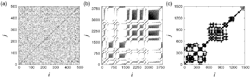
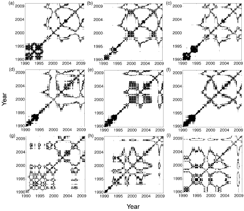
RPs capture the essential features of a system [30, 19]. RPs of three different types of data sets, viz., uniform white noise, chaotic Lorenz system, and daily financial data, are shown in Fig. 1. All three plots are distinct from each other and characteristic of the system.
Next, we give some measures to characterize RPs.
3.2 Probability of Recurrence
The Probability of Recurrence , also called the -recurrence rate, is the recurrence rate of a diagonal line situated at steps from the main diagonal, i.e., [19]. It is a probabilistic measure that gives the probability of an point falling in the -neighborhood of the point:
| (2) |
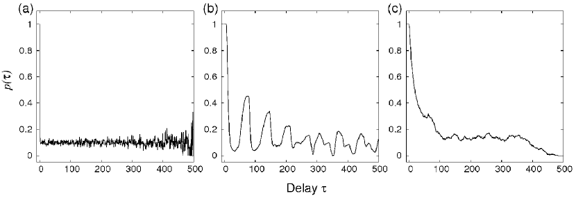
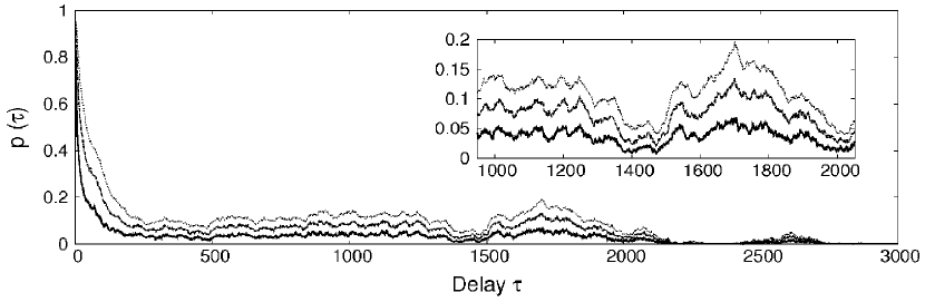
It can be considered as a generalized form of an autocorrelation function that statistically reflects the time scales of the system in which it tends to return to a previous configuration. For instance, the uniform white noise time series of Fig. 1(a) has almost the same probability of recurring to an earlier state for all values of (Fig. 2(a)), while the chaotic Lorenz system of Fig. 1(b) has periodic tendencies for high recurrences but with decreasing intensity (Fig. 2(b)), and the probabilities of recurrence for the daily DAX data from Fig. 1(c) decreases (without periodicities) with increase in , indicating the chances of a drift in the data set (Fig. 2(c)).
3.3 Correlation of Probability of Recurrence
The Correlation of Probability of Recurrence () is defined as the cross-correlation coefficient between the probabilities of recurrence of two trajectories and [20, 19]:
| (3) |
where represents the expectation value and is the series normalized to zero mean and standard deviation one (henceforth, ‘normalization’ refers to this particular way of normalizing a time series).
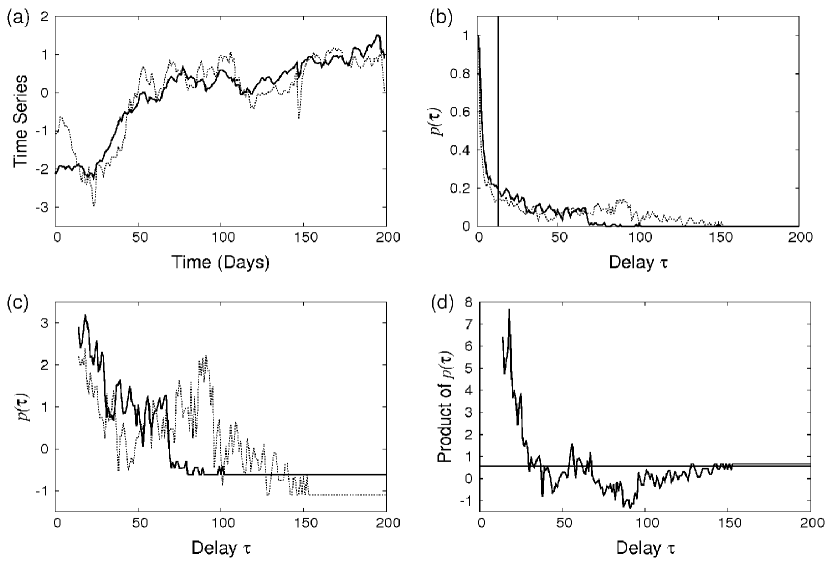
However, all the curves in Fig. 2 start from , because the recurrence rate is always 1 at , the main diagonal. This initial portion of the curve, common to all trajectories, introduce a bias towards a high value. To evaluate correctly, we suggest to consider only for such larger than the autocorrelation time of the system (defined as the delay at which the autocorrelation function of the system falls to ):
| (4) |
where
| (5) |
This is shown in Fig. 3 which illustrates the steps involved in estimating . The between the two time series according to Eq. (3) is 0.892, whereas it is 0.575 according to Eqs. (4) and (5).
characterizes the degree of phase synchronization between two time series, with implying that the two systems are phase synchronized [19]. However, it can be interpreted more generally as a measure denoting the level to which two trajectories and have similar time scales of recurrence. In this study, this means that two financial time series with a high tend to recur at similar times, suggesting some similarity in their underlying dynamics.
3.4 Pearson correlation
The Pearson correlation coefficient () is commonly used to analyze correlations between financial data. It is then used to define the distance between the data sets as given in [1]. It is simply the expectation value of the product of the normalized time series:
| (6) |
where and are the same as before.
3.5 Significance testing and Twin Surrogates
To use the alone for interpretations might be misleading. In an active experiment (such as laboratory experiments or numerical simulations of model systems) where the parameters of the system can be controlled, the for different parameter sets can be compared and thus, a consistent interpretation is possible. However, the financial time series we use are the only realizations of the black boxes generating them. In such a passive experiment, where the parameters of the system cannot be changed or controlled, or its dynamics are unknown, it is crucial to generate surrogate time series and check for the statistical significance of the observed against the distribution of obtained from the surrogate data sets. This is done using a statistical test and an appropriate null hypothesis.
The Twin Surrogates (TS) algorithm is a recurrence-based method of generating surrogate time series [26]. A pair of points and of a trajectory (of length ) are called twins if, for . This means that, barring their exact positions in the trajectory, these two points have the same neighborhood in phase space. The TS method is an iterative algorithm that involves:
-
i.
Identifying twins from the recurrence plot of the trajectory .
-
ii.
Taking any arbitrary point as the starting point of the surrogate trajectory .
-
iii.
Iteratively adding subsequent points to as: if is the previous point of , and has no twins, then the next point of is simply ; whereas if has twins, then the next point of is any one of that particular set of twins, chosen with equal probability.
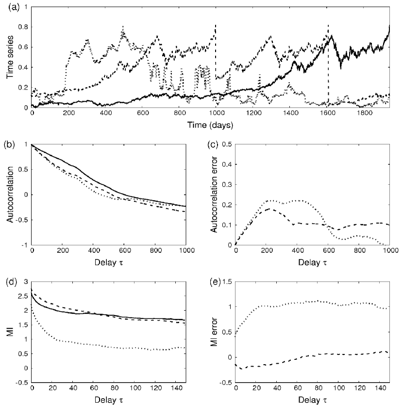
Although there are several methods to generate surrogate time series, it is natural to use TS in this study. In the widespread iterative Amplitude Adjusted Fourier Transform (iAAFT) method, surrogates are created with the assumed null hypothesis that the observed time series is the result of a Gaussian process seen through a static linear filter whereas, in TS, each surrogate is an independent realization of the observed time series differing only in the initial conditions. iAAFT surrogates do not preserve nonlinear characteristics such as mutual information, whereas TS preserves linear as well as nonlinear properties of a system [26]. Fig. 4(a) shows the original time series from DAX and both the surrogates via iAAFT and TS. Although the errors in autocorrelation for both methods are comparable, the iAAFT surrogate has much larger error in mutual information than the TS (Figs. 4(b)-(e)).
We use the TS to generate a test distribution using which we test the significance of the observed measure (which can be either or ). The null hypothesis for this significance test is that each surrogate is an independent trajectory of the same dynamical system which gave rise to the observed time series. This means that when we test for significance, we check for the probability that an independent realization of one of the time series (as given by its TS) can give a similar value of . The steps involved in the test are:
-
i.
The value of between time series A and B is estimated and designated as (say).
-
ii.
TS are generated from the series B.
-
iii.
is calculated between each surrogate and the series A. This gives the test distribution of . We assume that this distribution is roughly normal as each TS corresponds to a distinct trajectory of system B starting from an independent initial condition.
-
iv.
The mean and standard deviation are estimated for this test distribution.
-
v.
The test statistic is then evaluated as:
(7) which can be used to infer the probability with which belongs to a standard normal distribution.
A prefixed cut-off for the probability is decided below which is said to be significantly different from the test distribution, and this is the significance level of the test. The probability value (or -value) obtained from the standard normal table for the test statistic represents the probability that might actually be from the test distribution. In terms of the null hypothesis — that the two time series are independent — the -value represents the probability that the null hypothesis cannot be rejected.
4 Methods
4.1 The data set
The daily close values ranging from 3 December 1990 to 30 April 2010 of nine stock indices (given in Table 1) from around the world were used in our analysis. Three were from Asia, three from Europe and three from the U.S.A. The data was obtained from http://finance.yahoo.com/. Each data set contained a numerical value (representing the close value of the index on a particular date) and its corresponding date.
| Label | Stock Index | Location |
|---|---|---|
| A | CAC 40 | France |
| B | FTSE 100 | U.K. |
| C | DAX | Germany |
| D | NASDAQ | U.S.A |
| E | DJIA | U.S.A |
| F | S&P 500 | U.S.A |
| G | Nikkei 225 | Japan |
| H | Hang Seng | China |
| I | Strait Times | Singapore |
4.2 Preprocessing the data set
The data sets had unequal lengths because of the unequal distribution of holidays for stock indices in different regions of the world. To align them temporally, mismatched dates (and the corresponding close values) were deleted, i.e., any date of a particular market not present in any one (or more) other market(s) of the remaining eight resulted in the deletion of that date (and the corresponding close value) from all the markets. Simply put, a common intersect of all the nine data sets, in terms of dates, was obtained, which was of length 4238 time points.
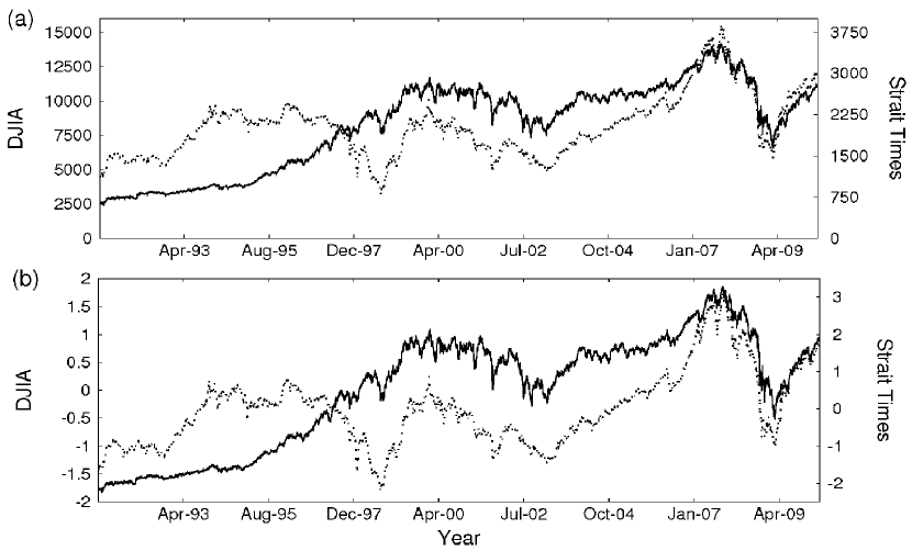
Moreover, the index values of the different indices were arbitrary (Fig. 5(a)). To make qualitative comparisons possible, they were normalized to mean zero and a standard deviation of one (Fig. 5(b)). This enabled us to compare the scaled time series and all the recurrence-based measures obtained from them using the same value of the parameters, e.g., the same value of the recurrence threshold .
4.3 Selection of parameters: Preliminary analysis
4.3.1 Window size
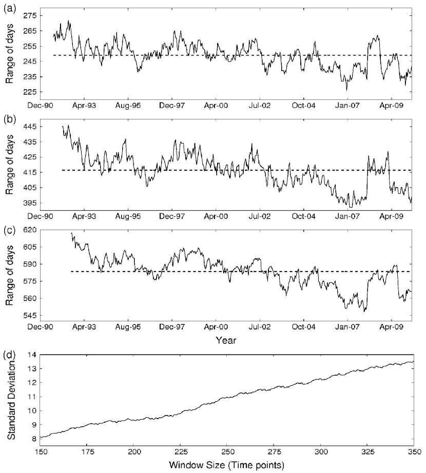
The primary method in this study is to slide a window of fixed width along the time series and then estimate or . However, because of the deletion of dates (see Sec. 4.2), if a window of, say, 500 consecutive time points is chosen, the actual range of days contained in it is larger than 500 and further, this range changes as the window moves along the time series (Fig. 6(a)-(c)). In order to get an understanding of the variation in the range of days contained in a window with respect to the number of time points in the window, we varied the window size from 150 to 350 time points and estimated the standard deviation of the range of days contained in each window, and found that the standard deviation increases (almost) monotonically with increasing window size (Fig. 6(d)).
Ideally, we want a window with negligible standard deviation. However, this would mean reducing the window size which would reduce the effectiveness of the RP and, in turn, the measures estimated from it. As a compromise, we choose a window of 250 time points, which is partly arbitrary but we (reasonably) assume that the qualitative features of the results are not severely effected by increasing or decreasing the window size from 250 by a small margin. The mean range of days contained in a 250 time point window is approximately 416 days, which is roughly equal to 19 months (considering a 5-day week).
4.3.2 RP parameters
There are several ways of constructing an RP from data [19], e.g., with a fixed threshold or a varying one, with or without embedding. In our analysis, we do not embed the time series. Also, there is no fixed rule to select . It depends on the objectives of the study and the nature of the data set. The choice of should ensure that the recurrence matrix represents the dynamics of the system. It should neither be too large (to avoid counting spurious recurrences) nor be too small (to avoid excluding crucial recurrences). One rule of thumb is to ensure that does not exceed 10% of the maximum distance between the points in the time series [31]. Another approach is to consider the recurrence-based measure as a signal detector and then choose the value that yields the maximum power from the signal for the detector being considered [32].
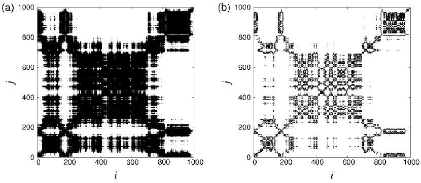
In our study we find that keeping of the maximum distance often results in a ‘dense’ RP (Fig. 7(a)). Therefore, to capture the finer recurrence structures while still allowing for sufficient statistics in the , we choose as the threshold for all RPs and normalize the time series (or any segments thereof) before the recurrence-based calculations. This effectively reduces the recurrence threshold to about of the maximum distance and gives a ‘clearer’ RP (Fig. 7(b)). The RPs given in Fig. 8 were obtained with , where it corresponds to around 2-3% of the maximum distance.
We find that the qualitative features of recurrences are robust to this choice of . In Fig. 9, the curves for the Hang Seng index obtained from its RP (Fig. 8(h)) are shown for and of the maximum distance. Although the magnitude of recurrences increases with increasing threshold, the qualitative nature of the curves remains the same throughout. The results obtained in this study are thus robust to small changes in .
4.4 Analyzing connectivity trends: Primary analysis
First, a window of 250 time points was moved along pairs of time series and the and values were estimated. This was done for all 36 pairs possible between the nine time series. Next, the values were binned in three categories:
(a) strong connectedness(),
(b) moderate connectedness(), and
(c) weak connectedness(),
and the number of connections (out of the 36) in each bin were counted for every window.
As a second step, the behavior of during the Dot-Com bubble in 2000 was considered, in which:
(a) taking a pair of time series, the dates when they peaked during the Dot-Com were made to coincide,
(b) a window of 250 time points was moved from 500 time points before the peak to 250 time points after, and
(c) the respective (or ) was obtained.
At every step, all (or ) values were tested for significance with 100 Twin Surrogates at 10% significance.
5 Results and Discussion
In this section, we present the main results obtained using the extended approach and the steps described in Sec. 4.4.
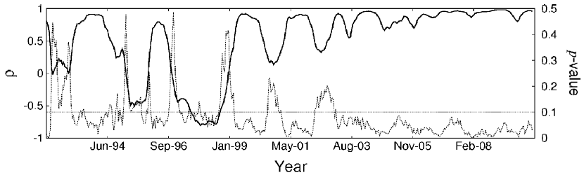
5.1 Trends in
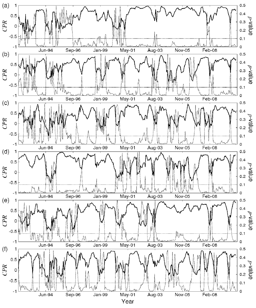
Three points are evident from Fig. 10 (which shows trends in for six pairs of indices along with the corresponding -values, viz., (a) CAC 40 and FTSE 100, (b) DAX and NASDAQ, (c) DAX and Nikkei 225, (d) DJIA and S&P 500, (e) S&P 500 and Strait Times, and (f) Nikkei 225 and Hang Seng).
-
i.
The does not have a monotonous trend over time. Rather it oscillates erratically with small periods of low interspersing broader bands of high .
-
ii.
The regions of low values have high -values (and vice versa), meaning that the lower ranges of tend to be less statistically significant in comparison to the higher values.
-
iii.
These patterns in the are same for all index pairs, of which only six are shown in Fig. 10.
Thus, if were to be interpreted as a measure of similarity, and hence connectedness, it means that the financial world is not moving monotonously to a globally connected scenario, but is rather oscillating between long periods of strong connectedness and short spans of low connectivity. (Nothing conclusive can be said about the nature of connections in the short periods of low as the estimates therein are not statistically significant.) In a sense, what it says is that the more things change the more they remain the same.
5.2 Patterns of connectivity
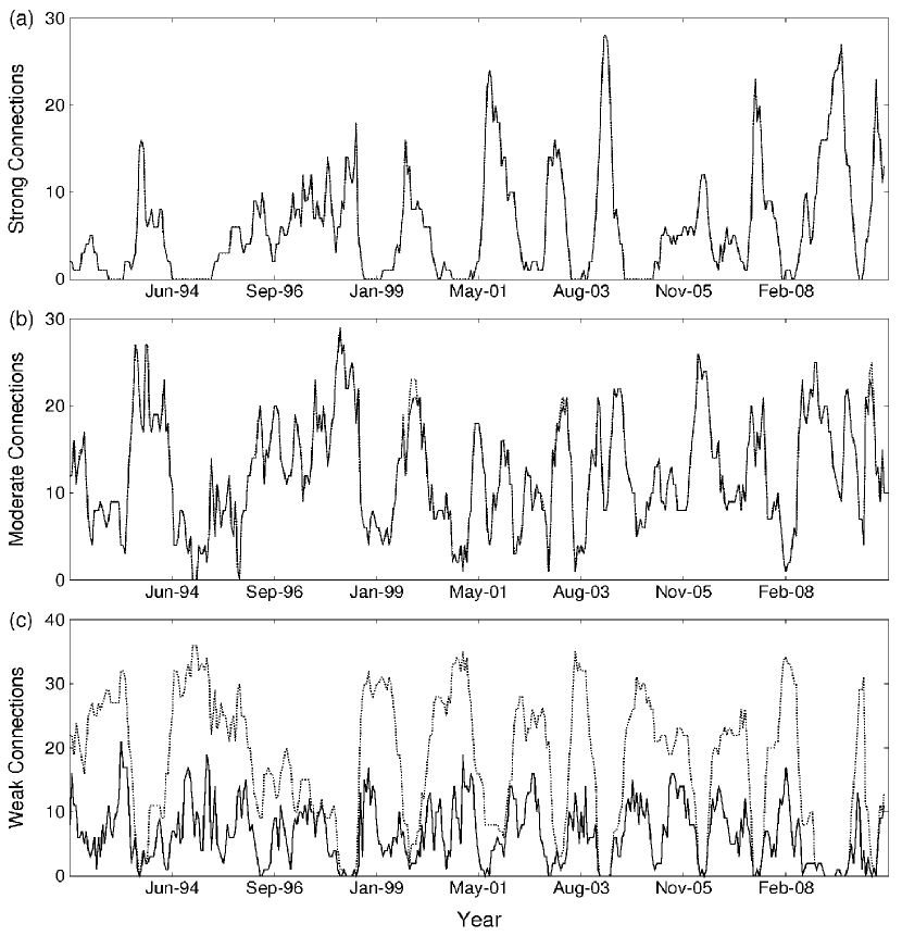
The patterns in the number of connections in each of the three bins, summed up among all pairs of indices, reinforce the picture put forth in Fig. 10. This is shown in Fig. 11. The strong and moderate connections are always statistically significant except for a few instances. The weak connections are clearly more prone to be statistically non-significant. Again, we see that there is no global trend in Fig. 11, i.e., there is no indication for an increasing global connectivity. Instead, we see that the number of strong and moderate connections oscillate erratically, implying that these nine indices come close to each other, and then move apart, and then come close again, and so on. Had all of them moved to higher connectivity over time, the number of connections in the strong category would have increased progressively, and the numbers in the other two bins would have gone down with it.
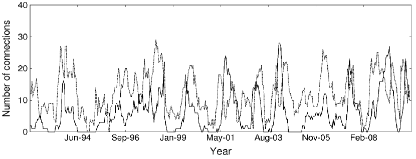
The strong and moderate connections move (loosely) in phase with each other (see Fig. 12). Starting from the dip in Jan-1999, consecutive dips occur roughly at Dec-2000, Jul-2002, Sep-2003, Feb-2005, Sep-2006, Feb-2008, and Oct-2009, meaning that the periods of these dips lie between 14 to 20 months. This might be indicative of the Kitchin business cycle [33].
Also, the number of ‘weak’ connections (Fig. 11(c)) is anti-phase to the number of ‘strong’ and ‘moderate’ connections (Figs. 11(a)-(b) and Fig. 12), because the total number of connections has to be conserved while the number in each of the three levels of connectedness go through cyclical patterns.
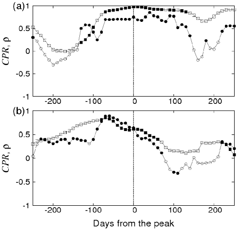
5.3 in the Dot-Com bubble
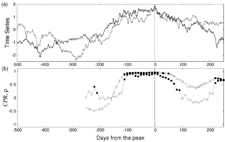
Figs. 13 and 14 give an insight into the way stock indices approach a crisis and then recede from it. Even though the indices peaked and crashed on distinct days (sometimes months apart), once the time series is shifted to align the peak-off dates (Fig. 13(a)), the increases around the peak-off date and decreases thereafter. For CAC 40 and Strait Times, the decrease in starts almost at the peak-off date (Fig. 13(b)). On the other hand, for DAX and NASDAQ it occurs after the peak-off date (Fig. 14(a)) and for NASDAQ and DJIA it happens before (Fig. 14(b)). The increase-and-decrease of is common to all of them. Thus, the probabilities of recurrence have strong correlation around the peak, i.e., irrespective of the actual date on which a particular index may peak, all indices approach and recede from a crisis similarly.
5.4 Trends in Pearson’s
The trend in Pearson’s is strongly different from , as shown for S&P 500 and Strait Times in Fig. 15 (which is the same pair as in Fig. 10(e)). Fig. 15 shows an overall movement towards higher correlation as time progresses, in contrast to the oscillating pattern of Fig. 10(e). The question then arises: which is the correct picture? Here, it is crucial to emphasize that these two measures capture different aspects of the time series. While measures the tendency of the time series values to move together in one direction (or opposite directions), measures the tendency of the time series values to return to earlier values at similar time scales. Hence, it is expected that their results are different. However, the case for can be interpreted as follows: being based on recurrence rates it captures the essential dynamical nature of the system. This is in contrast to Pearson’s which is simply a statistical comparison of co-evolution of states. Pearson’s is less sensitive to changes in the time series as pointed out earlier. Thus, while it may be true that stock indices tend to show more co-movement towards the latter half of our data sets, this does not necessarily imply that they will continue to do so as the corresponding system dynamics move in and out of strong periods of correlation (see Sec. 5.1).
5.5 Advantages of
We highlight the following advantages of as a measure for estimating connections between financial data sets.
-
i.
It is able to extract patterns even from noisy data sets, as is the case with most financial data. Moreover, it does not require that the data are distributed normally, as is required for the proper usage of .
-
ii.
The data sets need not be necessarily embedded for its estimation.
-
iii.
It can be estimated for short time series as well, as is done in the current work.
-
iv.
It does not require high-frequency sampling of the data, which is common in most financial analyses. Our analysis was done with daily sampled data which was freely available on the internet.
-
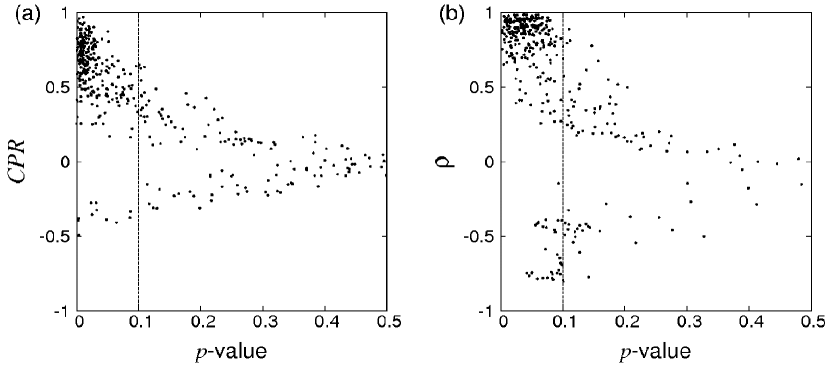
v.
It tends to have lower -values than , as seen from the spread of points in the top-left corners of the plots in Fig. 16. Most values are grouped close to the axis, whereas the values have a broader spread. This imples that the probability of rejecting the null hypothesis tends to be lower with .
6 Conclusion
In summary, we present a new way of looking at connections between different stock markets. This perspective, involving recurrences and , uncovers that, over the past two decades, markets have not proceeded towards an ever increasing connected state but rather moved in and out of strongly connected periods. It also points out that stock indices share similar dynamics during a bubble.
Moreover, we highlight the importance of significance testing, with the help of Twin Surrogates, in interpreting measures that analyze field data. In this respect, proves to be a robust measure and moreover, one having the power to reveal patterns from relatively poor data sets — in terms of noise, low frequency of sampling, and short time series length — even.
Lastly, we suggest a slight modification of the , which removes the problem of overestimation of coupling by it, thereby extending its capacity as a measure that can estimate connections between time series data effectively. This opens up newer possibilities of analyzing couplings between financial time series using (cross) recurrence analysis in a better manner.
Acknowledgments
B. Goswami thanks the Deutscher Akademischer Austausch Dienst (DAAD) for funding his internship at the Potsdam Institute for Climate Impact Research (PIK) under the Working Internships in Science and Engineering (WISE) program, wherein this study began. He also thanks Sutirth Dey and Deepak Barua for helpful discussions regarding significance testing and data representation. This work was also partly supported by the Federal Ministry of Education and Research, Germany, (project PROGRESS, 03IS2191B).
References
References
- [1] R. N. Mantegna, Hierarchical structure in financial markets, Eur. Phys. J. B 11 (1) (1999) 193–197.
- [2] R. N. Mantegna, H. E. Stanley, An Introduction to Econophysics: Correlations and Complexity in Finance, Cambridge University Press, 2000.
- [3] G. Bonanno, F. Lillo, R. N. Mantegna, Levels of complexity in financial markets, Physica A 299 (1-2) (2001) 16–27.
- [4] J.-P. Bouchaud, M. Potters, More stylized facts of financial markets: leverage effect and downside correlations, Physica A 299 (1-2) (2001) 60–70.
- [5] S. Drożdż, F. Grümmer, F. Ruf, J. Speth, Towards identifying the world stock market cross-correlations: DAX versus Dow Jones, Physica A 294 (1-2) (2001) 226–234.
- [6] J.-P. Onnela, A. Chakraborti, K. Kaski, J. Kertész, Dynamic asset trees and Black Monday, Physica A 324 (1-2) (2003) 247–252.
- [7] G. Bonanno, G. Caldarelli, F. Lillo, S. Miccichè, N. Vandewalle, R. N. Mantegna, Networks of equities in financial markets, Eur. Phys. J. B 38 (2) (2004) 363–371.
- [8] J. Kwapień, S. Drożdż, J. Speth, Time scales involved in emergent market coherence, Physica A 337 (1-2) (2004) 231–242.
- [9] D. Wilcox, T. Gebbie, On the analysis of cross-correlations in South African market data, Physica A 344 (1-2) (2004) 294–298.
- [10] T. Aste, T. D. Matteo, M. Tumminello, R. N. Mantegna, Correlation filtering in financial time series (Invited Paper), in: D. Abbott, J.-P. Bouchaud, X. Gabaix, J. McCauley (Eds.), Noise and Fluctuations in Econophysics and Finance, Vol. 5848 of Proc. SPIE, SPIE, Bellingham and WA, 2005, pp. 100–109.
- [11] J.-P. Onnela, J. Saramäki, K. Kaski, J. Kertész, Financial market - a network perspective, in: H. Takayasu (Ed.), Practical Fruits of Econophysics, Springer Tokyo, 2006, pp. 302–306.
- [12] R. Coelho, C. G. Gilmore, B. Lucey, P. Richmond, S. Hutzler, The evolution of interdependence in world equity markets—Evidence from minimum spanning trees, Physica A 376 (2007) 455–466.
- [13] R. Coelho, S. Hutzler, P. Repetowicz, P. Richmond, Sector analysis for a FTSE portfolio of stocks, Physica A 373 (2007) 615–626.
- [14] S. Çukur, M. Eryiğit, R. Eryiğit, Cross correlations in an emerging market financial data, Physica A 376 (2007) 555–564.
- [15] C. Eom, G. Oh, S. Kim, Deterministic factors of stock networks based on cross-correlation in financial market, Physica A 383 (1) (2007) 139–146.
- [16] M. Tumminello, C. Coronnello, F. Lillo, S. Miccichè, R. N. Mantegna, Spanning trees and bootstrap reliability estimation in correlation-based networks, Int. J. Bifurc. Chaos 17 (7) (2007) 2319–2329.
- [17] T. Conlon, H. J. Ruskin, M. Crane, Cross-correlation dynamics in financial time series, Physica A 388 (5) (2009) 705–714.
- [18] D. Y. Kenett, M. Tumminello, A. Madi, G. Gur-Gershgoren, R. N. Mantegna, E. Ben-Jacob, Dominating clasp of the financial sector revealed by partial correlation analysis of the stock market, PLoS ONE 5 (12) (2010) e15032.
- [19] N. Marwan, M. C. Romano, M. Thiel, J. Kurths, Recurrence plots for the analysis of complex systems, Phys. Rep. 438 (5-6) (2007) 237–329.
- [20] M. C. Romano, M. Thiel, J. Kurths, I. Z. Kiss, J. L. Hudson, Detection of synchronization for non-phase-coherent and non-stationary data, Europhys. Lett. 71 (3) (2005) 466–472.
- [21] F. Strozzi, J.-M. Zaldívar, J. P. Zbilut, Application of nonlinear time series analysis techniques to high-frequency currency exchange data, Physica A 312 (3-4) (2002) 520–538.
- [22] K. Guhathakurta, B. Bhattacharya, A. R. Chowdhury, Using recurrence plot analysis to distinguish between endogenous and exogenous stock market crashes, Physica A 389 (9) (2010) 1874–1882.
- [23] A. Fabretti, M. Ausloos, Recurrence analysis near the NASDAQ crash of April 2000, in: H. Takayasu (Ed.), Practical Fruits of Econophysics, Springer Tokyo, 2006, pp. 52–56.
- [24] J. A. Bastos, J. Caiado, Recurrence quantification analysis of global stock markets, Physica A 390 (7) (2011) 1315–1325.
- [25] P. M. Crowley, Analyzing convergence and synchronicity of business and growth cycles in the euro area using cross recurrence plots, Eur. Phys. J. Spec. Top. 164 (1) (2008) 67–84.
- [26] M. Thiel, M. C. Romano, J. Kurths, M. Rolfs, R. Kliegl, Twin surrogates to test for complex synchronisation, Europhys. Lett. 75 (4) (2006) 535–541.
- [27] J. Imbs, Trade, finance, specialization, and synchronization, Rev. Econ. Stat. 86 (3) (2004) 723–734.
- [28] C. W. J. Granger, Some properties of time series data and their use in econometric model specification, J. Econom. 16 (1) (1981) 121–130.
- [29] R. F. Engle, C. W. J. Granger, Co-integration and error correction: Representation, estimation, and testing, Econometrica 55 (2) (1987) 251–276.
- [30] J.-P. Eckmann, S. O. Kamphorst, D. Ruelle, Recurrence plots of dynamical systems, Europhys. Lett. 4 (9) (1987) 973–977.
- [31] J. P. Zbilut, C. L. Webber, Jr., Embeddings and delays as derived from quantification of recurrence plots, Phys. Lett. A 171 (3-4) (1992) 199–203.
- [32] S. Schinkel, O. Dimigen, N. Marwan, Selection of recurrence threshold for signal detection, Eur. Phys. J. Spec. Top. 164 (1) (2008) 45–53.
- [33] J. Kitchin, Cycles and trends in economic factors, Rev. Econ. Stat. 5 (1) (1923) 10–16.