Summation-By-Parts Operators and High-Order Quadrature

Abstract

Summation-by-parts (SBP) operators are finite-difference operators that mimic integration by parts. This property can be useful in constructing energy-stable discretizations of partial differential equations. SBP operators are defined by a weight matrix and a difference operator, with the latter designed to approximate $d/dx$ to a specified order of accuracy. The accuracy of the weight matrix as a quadrature rule is not explicitly part of the SBP definition. We show that SBP weight matrices are related to trapezoid rules with end corrections whose accuracy matches the corresponding difference operator at internal nodes. The accuracy of SBP quadrature extends to curvilinear domains provided the Jacobian is approximated with the same SBP operator used for the quadrature. This quadrature has significant implications for SBP-based discretizations; for example, the discrete norm accurately approximates the $L^{2}$ norm for functions, and multi-dimensional SBP discretizations accurately mimic the divergence theorem.

1 Introduction

Partial differential equations (PDEs) are often solved numerically in order to approximate a functional that depends on the solution; for example, when computational fluid dynamics is used to estimate the lift and drag on an aerodynamic body. For integral functionals, such as lift and drag, a quadrature rule may be needed to numerically integrate the discrete solution. When we are free to choose the quadrature weights and abscissas, Guassian quadrature is often the optimal choice. However, the choice of quadrature rule is less clear for the uniform grids that arise in finite-difference methods.

In this paper, we investigate a quadrature rule that is particularly well suited for high-order summation-by-parts (SBP) finite-difference methods [1]. SBP operators lead to linearly time-stable discretizations of well-posed PDEs, and they have been used to construct efficient discretizations of the Euler [2, 3], Navier-Stokes [4, 5, 6], and Einstein equations [7]. The high-order quadrature in question is based on the weight matrix that forms part of the definition of SBP operators. This result is somewhat surprising, because the accuracy of the quadrature induced by the weight matrix is not explicitly part of the SBP definition. To our knowledge, the relationship between SBP operators and quadrature has not been discussed previously in the literature.

In the context of high-order finite-difference methods, including those based on SBP operators, several classical quadrature rules are available to accurately evaluate integral functionals; for example, composite Newton-Cotes rules and Gregory-type formulae. Why introduce a new quadrature rule based on SBP weight matrices? While accuracy is important, we may also want the functional estimate to obey some property or properties of the true functional, and this is the value of SBP-based quadrature.

Consider the volume integral of the divergence of a vector field over a compact domain. The resulting functional is equivalent to the flux of the vector field over the domain’s boundary, in light of the divergence theorem. This is a fundamental property of the functional that we may want a discretization and quadrature to preserve. We say a functional estimate respects, or mimics, the divergence theorem if 1) it is accurate, and 2) the discrete quadrature over the volume produces a discrete quadrature over the surface.

In general, classical quadrature rules for uniformly spaced data will not mimic the divergence theorem in the above sense when applied to an arbitrary high-order finite-difference approximation of the divergence; typically, they will satisfy the first but not the second property. In contrast, we will show that an SBP discretization does mimic the divergence theorem when numerically integrated using its corresponding weight matrix.

The paper is organized as follows. Section 2 introduces notation and formally defines SBP operators. Section 3 presents the main theoretical results. In particular, we derive conditions on the quadrature weights for the class of trapezoid rules with end corrections. These conditions are used to establish the accuracy of SBP-based quadrature. Subsequently, we consider the impact of coordinate transformations on SBP quadrature and show that the quadrature remains accurate on curvilinear multi-dimensional domains. In Section 4 we verify the theoretical results with several numerical examples. The implications of SBP quadrature are summarized and discussed in Section 5.

2 Notation and definitions

We try to remain consistent with the notation used by Kreiss and Scherer in their original work [1], as well as Strand’s subsequent work [8].

The interval $[0,1]$ is partitioned into $n+1$ evenly spaced points $x_{v}=vh,\;v=0,1,\ldots,n$, with mesh spacing $h=1/n$. Finite intervals other than $[0,1]$, as well as nonuniform node spacing, can be accommodated by introducing an appropriate mapping (see Section 3.2). For arbitrary $\mathcal{U}(x)\in C^{p}[0,1]$, we use $u_{v}=\mathcal{U}(x_{v})$ to denote the restriction of $\mathcal{U}$ to the grid $x_{v}$.

Definition 1 (Summation-By-Parts Operator)

The matrix $D\in\mathbb{R}^{(n+1)\times(n+1)}$ is a summation-by-parts operator for the first derivative on the mesh $\{x_{v}\}_{v=0}^{n}$ if it has the form

$$D=H^{-1}Q,$$

where the weight matrix $H\in\mathbb{R}^{(n+1)\times(n+1)}$ is a symmetric-positive-definite matrix, and $Q\in\mathbb{R}^{(n+1)\times(n+1)}$ satisfies

$$Q+Q^{T}=\operatorname{diag}{(-1,0,0,\ldots,1)}.$$

Furthermore, the truncation error of the difference operator $D$ in approximating $d/dx$ is order $h^{2s}$ at the internal nodes, $\{x_{v}\}_{v=r}^{n-r}$, and order $h^{\tau}$ at the boundary nodes, $\{x_{v}\}_{v=0}^{r-1}$ and $\{x_{v}\}_{v=n-r+1}^{n}$, where $\tau,r,s\geq 1$.

In other words, the SBP operator $D$ approximates $d/dx$ and has a particular structure. In general, the order of accuracy of the difference stencil at internal nodes is different than the order of accuracy of the stencil at boundary nodes. The even order of accuracy $2s$ for the internal nodes is a consequence of using centered-difference schemes, which provide the lowest error for a given stencil size. For a $2s$-order accurate scheme, the derivative at the internal nodes is approximated as

$$\frac{d\mathcal{U}}{dx}(x_{w}) \approx\sum_{v=1}^{s}\frac{\alpha_{v}}{h}(u_{w+v}-u_{w-v}),\qquad r\leq w\leq n-r,$$

where the coefficients are defined by (see [9], for example)

$$\alpha_{v} =\frac{(-1)^{v+1}(s!)^{2}}{v(s+v)!(s-v)!}.$$

The following lemma from [8] lists some identities that the $\alpha_{v}$ satisfy; these identities will be useful in our subsequent analysis.

Lemma 1

The coefficients $\alpha_{v}$ that define a $2s$-order accurate SBP operator at internal nodes satisfy

$$\sum_{v=1}^{s}\alpha_{v}v^{2j+1}=\begin{cases}\frac{1}{2},&j=0,\\ 0,&j=1,2,\ldots,s-1.\end{cases}$$

We turn our attention to the weight matrix $H$, which is the focus of this paper. Since $H$ is symmetric-positive-definite, we can use it to define an inner product and corresponding norm for vectors. Let $u,z\in\mathbb{R}^{n+1}$ be two discrete functions on the grid nodes, i.e. $u_{v}=\mathcal{U}(x_{v})$ and $z_{v}=\mathcal{Z}(x_{v})$. Then

$$(u,z)_{H}\equiv u^{T}Hz,\quad\text{and }\quad\|u\|_{H}^{2}\equiv(u,u)_{H},$$

define the $H$ inner product and $H$ norm, respectively. Using the SBP-operator definition and the $H$ inner product, we have

$$(u,D\,z)_{H}=-(D\,u,z)_{H}-u_{0}z_{0}+u_{n}z_{n}.$$ (1)

Equation (1) expresses the fundamental property of SBP operators and is the discrete analog of

$$\int_{a}^{b}\mathcal{U}\frac{d\mathcal{Z}}{dx}dx=-\int_{a}^{b}\mathcal{Z}\frac{d\mathcal{U}}{dx}dx+\left.\mathcal{U}\mathcal{Z}\right|_{x=a}^{x=b}.$$ (2)

This property of SBP operators is what leads to energy-stable discretizations of partial differential equations. However, while (1) is analogous to integration by parts, it remains to be shown that (1) is an accurate discretization of (2).

In this work, we will consider $H$ matrices with the block structure

$$H=h\begin{pmatrix}H_{L}&0&0\\ 0&I&0\\ 0&0&H_{R}\end{pmatrix},$$ (3)

where $H_{L},H_{R}\in\mathbb{R}^{r\times r}$ are symmetric-positive-definite matrices. Assuming that $H_{L}$ and $H_{R}$ are dense matrices — the so-called full-norm case — Kreiss and Scherer [1] established the existence of SBP operators that achieve an order of accuracy of $\tau=2s-1$ at the boundary with $r=2s$. Strand [8] showed that $2s-1$ accuracy can be maintained at the boundary in the case of a restricted-full norm, which uses

$$H_{L}=\begin{pmatrix}h_{00}&0\\ 0&\bar{H}_{L}\end{pmatrix}\quad\text{and }\quad H_{R}=\begin{pmatrix}\bar{H}_{R}&0\\ 0&h_{00}\end{pmatrix}$$

with $\bar{H}_{L},\bar{H}_{R}\in\mathbb{R}^{(r-1)\times(r-1)}$ and $r=2s+1$.

In general, SBP weight matrices of the form (3) satisfy the compatibility conditions described in the following proposition [1]; these conditions will be used later to establish the accuracy of quadrature rules based on full and restricted-full $H$ matrices.

Proposition 1

Let $H\in\mathbb{R}^{(n+1)\times(n+1)}$ be an SBP weight matrix with the block structure (3). Then $H_{L}$ satisfies

$$je_{i}^{T}H_{L}e_{j-1}+ie_{j}^{T}H_{L}e_{i-1}=-(-r)^{i+j}+J_{i,j},\qquad 0\leq i,\,j\leq\tau,$$

where $e_{j}^{T}\equiv(-1)^{j}\begin{pmatrix}r^{j}&(r-1)^{j}&\cdots&1^{j}\end{pmatrix}$, with the convention $e_{-1}=0$, and

$$J_{i,j}=\sum_{v=1}^{s}\alpha_{v}\left[\sum_{w=0}^{v-1}w^{j}(w-v)^{i}+w^{i}(w-v)^{j}\right],\qquad i+j\geq 1.$$

Kreiss and Scherer also showed that it is possible to define SBP operators with diagonal $H$ matrices, i.e.

$$H_{L} =\operatorname{diag}{(\lambda_{0},\lambda_{1},\ldots,\lambda_{r-1})}$$

$$H_{R} =\operatorname{diag}{(\lambda_{r-1},\ldots,\lambda_{1},\lambda_{0})}$$

with $\lambda_{i}>0$. These “diagonal norms” are important because, unlike full and restricted-full norms, they lead to provably stable PDE discretizations on curvilinear grids [10]. However, diagonal-norm SBP operators are limited to $\tau=s$ accuracy at the boundary when the internal accuracy is $2s$. Consequently, the solution accuracy of hyperbolic systems discretized with such SBP operators is limited to order $s+1$ [11]. Nevertheless, one can show that functionals based on the solution of dual consistent diagonal-norm SBP discretizations are $2s$-order accurate [12, 13].

When the weight matrix $H$ is diagonal, Kreiss and Scherer [1] showed that its elements are defined by the relations in following proposition.

Proposition 2

Let $H\in\mathbb{R}^{(n+1)\times(n+1)}$ be a diagonal SBP weight matrix with $r=2\tau=2s$. Then the diagonal elements $\lambda_{v}$ of $H_{L}$ and $H_{R}$ satisfy the relations

$$j\sum_{v=0}^{r-1}\lambda_{v}(r-v)^{j-1}=\begin{cases}\phantom{2\sum_{v=1}^{s}}(r)^{j}-(-1)^{j}\beta_{j},&j=1,2,\ldots,2s-1\\ (r)^{2s}-2\sum_{v=1}^{s}\alpha_{v}\sum_{w=0}^{v-1}w^{s}(w-v)^{s},&j=2s,\end{cases}$$

where $\beta_{j}$ is the $j^{\text{th}}$ Bernoulli number.

3 Theory

3.1 One-dimensional SBP Quadrature

To establish the accuracy of SBP-based quadratures, we need the following theorem that places constraints on the coefficients of a certain class of quadrature rules for uniformly spaced data; specifically, the trapezoid rule with end corrections. The theorem is a direct consequence of substituting finite-difference approximations into the Euler-Maclaurin sum formula.

Theorem 1

Consider a set of $n+1$ uniformly spaced points, $x_{v}=vh,\;v=0,1,\ldots,n$, with constant mesh spacing $h=1/n$. A quadrature of the form

$$\mathcal{I}(u)\equiv h\left(\sum_{v=0}^{r-1}\sigma_{v}u_{v}+\sum_{v=r}^{n-r}u_{v}+\sum_{v=0}^{r-1}\sigma_{v}u_{n-v}\right)$$

is a $q$-order accurate approximation of $\int_{0}^{1}\mathcal{U}\,dx$ for $\mathcal{U}\in C^{2m+2}[0,1]$, where $q-1\leq r$ and $q\leq 2m+2$, if and only if the coefficients $\{\sigma_{v}\}_{v=0}^{r-1}$ satisfy

$$j\sum_{v=0}^{r-1}\sigma_{v}(r-v)^{j-1}=r^{j}-(-1)^{j}\beta_{j},\qquad j=1,2,\ldots,q-1,$$ (4)

Proof 1

Consider the Euler-Maclaurin sum formula applied to $\mathcal{U}(x)$ [14]:

$$\int_{0}^{1}\mathcal{U}(x)\,dx =h\sum_{v=0}^{n}u_{v}+\sum_{k=1}^{2m}\frac{\beta_{k}}{k!}h^{k}\left(u^{(k-1)}_{0}-(-1)^{k}u^{(k-1)}_{n}\right)+E_{2m},$$ (5)

where $$u^{(k-1)}_{v}\equiv D^{(k-1)}\mathcal{U}(x_{v}) 2m<q\leq 2m+2$$, , and the error term is given by

$$E_{2m} =\frac{\beta_{2m+2}h^{2m+2}}{(2m+2)!}D^{(2m+2)}\mathcal{U}(\xi),$$

with $\xi\in(0,1)$. Suppose the function derivatives at $x=0$ and $x=1$ are replaced with finite-difference approximations involving the first $r$ and last $r$ internal points, respectively. Moreover, assume that the approximation to $u_{v}^{(k-1)}$ is accurate to $\text{O}(h^{q-k})$, where $q-1\leq r$; consequently, the approximations are exact for polynomials up to at least degree $q-1$. Let $\{\delta_{v}^{(k-1)}\}_{v=0}^{r-1}$ denote the coefficients defining the finite-difference approximation of $u_{0}^{(k-1)}$, such that

$$u^{(k-1)}_{0}=\sum_{v=0}^{r-1}\frac{\delta_{v}^{(k-1)}}{h^{k-1}}u_{v}+\text{O}(h^{q-k}).$$

Substituting the finite-difference approximations into (5), and noting that the coefficients for odd derivatives must be negated at $x=1$, we find

$$\int_{0}^{1}\mathcal{U}(x)\,dx =h\sum_{v=0}^{n}u_{v}+\sum_{k=1}^{2m}\frac{\beta_{k}}{k!}h^{k}\sum_{v=0}^{r-1}\frac{\delta_{v}^{(k-1)}}{h^{k-1}}\left(u_{v}+u_{n-v}\right)+\text{O}(h^{q})+\text{O}(h^{2m+2})$$

$$=h\left(\sum_{v=0}^{r-1}\sigma_{v}u_{v}+\sum_{v=r}^{n-r}u_{v}+\sum_{v=0}^{r-1}\sigma_{v}u_{n-v}\right)+\text{O}(h^{q})$$

where

$$\sigma_{v}=1+\sum_{k=1}^{2m}\frac{\beta_{k}}{k!}\delta_{v}^{(k-1)},\qquad v=0,1,\ldots,r-1.$$ (6)

Next, we will show that these $\sigma_{v}$ are the same ones that satisfy (4), a set of $q-1$ conditions that are independent of the $\delta_{v}^{(k)}$. Substituting the above expression for $\sigma_{v}$ into (4), we find

$$j\sum_{v=0}^{r-1}\sigma_{v}(r-v)^{j-1}=j\sum_{v=0}^{r-1}(r-v)^{j-1}+j\sum_{k=1}^{2m}\frac{\beta_{k}}{k!}\sum_{v=0}^{r-1}\delta_{v}^{(k-1)}(r-v)^{j-1},\\ j=1,2,\ldots,q-1.$$ (7)

The first term on the right-hand side can be recast using the sum of powers formula:

$$j\sum_{v=0}^{r-1}(r-v)^{j-1}=r^{j}+\sum_{k=1}^{j-1}(-1)^{k}\binom{j}{k}\beta_{k}r^{j-k}.$$ (8)

For the second term, we recognize that $(r-v)^{j-1}$ is the discrete representation of the polynomial $p_{j-1}(x)\equiv h^{-(j-1)}(rh-x)^{j-1}$; therefore, since the finite-difference approximations are exact for polynomials of degree $q-1$, we have

$$\sum_{v=0}^{r-1}\delta_{v}^{(k-1)}(r-v)^{j-1}=\begin{cases}(-1)^{k-1}\frac{(j-1)!}{(j-k)!}r^{j-k},&k\leq j\\ 0,&k>j,\end{cases}$$

and

$$j\sum_{k=1}^{2m}\frac{\beta_{k}}{k!}\sum_{v=0}^{r-1}\delta_{v}^{(k-1)}(r-v)^{j-1}=\sum_{k=1}^{j}(-1)^{k-1}\binom{j}{k}\beta_{k}r^{j-k}.$$ (9)

Substituting (8) and (9) into (7), and recalling that the odd Bernoulli numbers greater than one are zero, we have

$$j\sum_{v=0}^{r-1}\sigma_{v}(r-v)^{j-1} =r^{j}+\sum_{k=1}^{j-1}(-1)^{k}\binom{j}{k}\beta_{k}r^{j-k}+\sum_{k=1}^{j}(-1)^{k-1}\binom{j}{k}\beta_{k}r^{j-k}$$

$$=r^{j}-(-1)^{j}\beta_{j},$$

for $j=1,2,\ldots,q-1$. Thus, we have shown that the $\sigma_{v}$ satisfy (4) when the quadrature is $q$-order accurate.

We need the general solution of (4) to show that these conditions are sufficient for the quadrature to be $q$-order accurate. We have already shown that (6) is a particular solution of the linear equations (4), so we need to determine the form of the homogeneous solution, i.e. the null space of the matrix on the left side of (4).

As noted above, $(r-v)^{j-1}$ is simply the polynomial $p_{j-1}(x)=h^{-(j-1)}(rh-x)^{j-1}$ evaluated at the nodes. The derivative operator $D^{(k-1)}$ with $q\leq k\leq r$ will annihilate $p_{j-1}(x)$, since $j\leq q-1$; therefore, any finite difference approximation that is a consistent approximation of $h^{k-1}D^{(k-1)}$, $q\leq k\leq r$, will annihilate $p_{j-1}(x_{v})=(r-v)^{j-1}$. If we let $\{\mu_{v}^{(k-1)}\}_{v=0}^{v=r-1}$ denote the coefficients of such a finite difference approximation, then the general solution to (4) can be written as

$$\sigma_{v}=1+\sum_{k=1}^{2m}\frac{\beta_{k}}{k!}\delta_{v}^{(k-1)}+\sum_{k=q}^{r}\gamma_{k-q}\mu_{v}^{(k-1)},$$ (10)

where $\{\gamma_{0},\gamma_{1},\ldots,\gamma_{r-q}\}$ parameterizes the null space. When $r=q-1$, the null space is trivial, and the second sum does not appear in (10).

Substituting the general solution into the quadrature yields

$$\mathcal{I}(u) =h\left(\sum_{v=0}^{r-1}\sigma_{v}u_{v}+\sum_{v=r}^{n-r}u_{v}+\sum_{v=0}^{r-1}\sigma_{v}u_{n-v}\right)$$

$$=h\sum_{v=0}^{n}u_{v}+\sum_{k=1}^{2m}\frac{\beta_{k}}{k!}h^{k}\sum_{v=0}^{r-1}\frac{\delta_{v}^{(k-1)}}{h^{k-1}}\left(u_{v}+u_{n-v}\right)$$

$$\phantom{=h\sum_{v=0}^{n}u_{v}}\qquad+h\sum_{k=q}^{r}\gamma_{k-q}\sum_{v=0}^{r-1}\mu_{v}^{(k-1)}(u_{v}+u_{n-v})$$

$$=\int_{0}^{1}\mathcal{U}(x)\,dx+\text{O}(h^{q})+\sum_{k=q}^{r}\gamma_{k-q}h^{k}\left(u_{0}^{(k-1)}+(-1)^{k}u_{n}^{(k-1)}\right)$$

$$=\int_{0}^{1}\mathcal{U}(x)\,dx+\text{O}(h^{q}).$$

Therefore, we have shown that (4) is sufficient for the quadrature to be $q$-order accurate, which completes the proof.

If we choose $q-1=r$, Theorem 1 provides a closed set of equations for constructing high-order quadrature rules for uniformly spaced data with equal weights on the internal points. More generally, we may choose $q-1<r$, in which case the additional degrees of freedom can be used to achieve other objectives. For example, setting $\sigma_{0}$ to zero, so that only strictly internal points are used.

Theorem 1 encompasses many existing quadrature rules, including the Gregory class of formulae, and it could be used to construct an unlimited number of novel trapezoid rules with end corrections. However, our interest in Theorem 1 is not in constructing new quadrature rules, but in its consequences for SBP weight matrices.

Corollary 1

Let $H$ be a full, restricted-full, or diagonal weight matrix from an SBP first-derivative operator $D=(H^{-1}Q)$, which is a $2s$-order-accurate approximation to $d/dx$ in the interior. Then the $H$ matrix constitutes a $2s$-order-accurate quadrature for integrands $\mathcal{U}\in C^{2s}$.

Proof 2

For diagonal SBP weight matrices the result follows immediately from Proposition 2, since (4), with $q=2s$, is a subset of the equations that define the $\lambda_{v}$. For the full and restricted-full weight matrices, consider the relations in Proposition 1 with $j\leq\tau=2s-1$ and $i=0$:

$$j\sum_{v=0}^{r-1}\sum_{w=0}^{r-1}h_{vw}(-1)^{j-1}(r-w)^{j-1}=-(-r)^{j}+\sum_{v=1}^{s}\alpha_{v}\sum_{w=0}^{v-1}\left[w^{j}+(w-v)^{j}\right].$$

Multiplying the left and right sides by $(-1)^{j-1}$, using the symmetry of the $h_{vw}$, and swapping summation indices on the left side, we find

$$j\sum_{v=0}^{r-1}\sigma_{v}(r-v)^{j-1}=r^{j}+(-1)^{j-1}\sum_{v=1}^{s}\alpha_{v}\sum_{w=0}^{v-1}\left[w^{j}+(w-v)^{j}\right],$$

where $\sigma_{v}$ is identified with $\sum_{w=0}^{r-1}h_{vw}$. The second term on the right-hand side can be simplified using the accuracy conditions of the $\alpha_{v}$ (Lemma 1) and the formula for the sum of powers.

$$\sum_{v=1}^{s}\alpha_{v}\sum_{w=0}^{v-1}\left[w^{j}+(w-v)^{j}\right] =\sum_{v=1}^{s}\alpha_{v}\left[-v^{j}+\sum_{w=1}^{v}w^{j}+(-1)^{j}\sum_{w=1}^{v}w^{j}\right]$$

$$=\sum_{v=1}^{s}\alpha_{v}\left[-v^{j}+\frac{(1+(-1)^{j})}{j+1}\sum_{w=0}^{j}\binom{j+1}{w}\beta_{w}v^{j+1-w}\right]$$

$$=\begin{cases}-\frac{1}{2},&j=1\\ \phantom{-}0,&j=3,5,\ldots,\tau,\\ \phantom{-}\beta_{j},&j=2,4,\ldots,\tau-1\end{cases}$$

$$=\beta_{j}.$$

Thus, we have

$$j\sum_{v=0}^{r-1}\sigma_{v}(r-v)^{j-1}=r^{j}-(-1)^{j}\beta_{j},\qquad 1\leq j\leq\tau,$$

and Theorem 1 implies that full and restricted-full SBP weight matrices are quadrature rules accurate to $\tau+1=2s$.

3.2 SBP Quadrature and Coordinate Transformations

Curvilinear coordinate systems are often necessary when solving PDEs on complex domains. Like most finite-difference schemes, SBP operators are not applied directly to the nodes in physical space. Instead, a coordinate transformation is used to map points in the physical domain to points on a Cartesian grid, and the SBP operators are applied in this uniform computational space. However, this coordinate transformation introduces geometric terms whose impact on the accuracy of the quadrature rule is not clear.

We begin by considering the one-dimensional case. Let $\mathcal{T}(x)=\xi(x)$ be an invertible transformation of class $C^{2s}$ that maps $\Omega_{x}=[a,b]$ to $\Omega_{\xi}=[0,1]$. For $\mathcal{U}\in L^{2}(\Omega_{x})$, the change of variable theorem implies

$$\int_{a}^{b}\mathcal{U}\,dx=\int_{0}^{1}\mathcal{U}\mathcal{J}\,d\xi,$$ (11)

where $\mathcal{J}=\frac{dx}{d\xi}$ is the Jacobian of $\mathcal{T}^{-1}$.

We are interested in the accuracy of SBP quadrature in the computational domain, so we consider the discrete equivalent of the right-hand side of (11). In general the mapping will not be explicitly available, so the Jacobian must be approximated. As we shall see, to retain the $2s$-order accuracy of SBP quadrature, it is critical that the derivative that appears in the Jacobian be approximated by the same SBP difference operator that defines the norm. Thus, if $x\in\mathbb{R}^{n+1}$ denotes the coordinates of the nodes in physical space, the SBP approximation of (11) is given by

$$u^{T}HDx=u^{T}Qx.$$ (12)

The following theorem confirms that this discrete product is a $2s$-order accurate approximation of the integral (11).

Theorem 2

Let $D=H^{-1}Q$ be an SBP first derivative operator. Then

$$(z,Du)_{H}=z^{T}Qu$$

is a $2s$-order-accurate approximation to the integral

$$\int_{0}^{1}\mathcal{Z}\frac{d\mathcal{U}}{dx}\,dx,$$

where $\mathcal{Z}\frac{d\mathcal{U}}{dx}\in C^{2s}[0,1]$.

Proof 3

Using SBP-norm quadrature we have

$$\int_{0}^{1}\mathcal{Z}\frac{d\mathcal{U}}{dx}\,dx=(z,u^{\prime})_{H}+\text{O}(h^{2s}),$$

where $u^{\prime}$ denotes the analytical derivative $\partial\mathcal{U}/\partial x$ evaluated at the grid nodes. The result will follow if we can show that

$$(z,u^{\prime})_{H}=(z,Du)_{H}+\text{O}(h^{2s}).$$ (13)

The expression on the left of (13) is simply a quadrature for the integrand $\mathcal{Y}=\mathcal{Z}\frac{d}{dx}\mathcal{U}$. Consequently, it is sufficient to show (13) is exact for polynomial integrands of degree less than $2s$. Let

$$w_{i}=\begin{bmatrix}x_{0}^{i}&x_{1}^{i}&\cdots&x_{n}^{i}\end{bmatrix}^{T}$$

be the restriction of the monomial $x^{i}$ to the grid. We will consider

$$z=w_{i},\quad u=w_{j},\quad\text{and}\qquad u^{\prime}=jw_{j-1},$$

with $i+j\leq 2s$.

First, suppose $j\leq s$. In this case, an SBP operator (including those with diagonal-norms) is exact for $w_{j}$ giving

$$Du=Dw_{j}=jw_{j-1}=u^{\prime},$$

and substitution into (13) yields $(z,u^{\prime})_{H}=(z,Du)_{H}$.

Next, to show that (13) is exact for $j>s$, the roles of $z$ and $u$ will be reversed. Here, since $j+i\leq 2s$, we must have $i<s$, and the SBP operator becomes exact for $w_{i}$:

$$Dz=Dw_{i}=iw_{i-1}=z^{\prime}.$$

Using this exact derivative and the properties of SBP operators we find

$$(z,Du)_{H} =z^{T}H(H^{-1}Q)u$$

$$=z_{n}u_{n}-z_{0}u_{0}-z^{T}Q^{T}u$$

$$=\left.\mathcal{U}\mathcal{Z}\right|_{x=1}-\left.\mathcal{U}\mathcal{Z}\right|_{x=0}-(u,Dz)_{H}$$

$$=\left.\mathcal{U}\mathcal{Z}\right|_{x=1}-\left.\mathcal{U}\mathcal{Z}\right|_{x=0}-(u,z^{\prime})_{H}$$

$$=\int_{0}^{1}\frac{d}{dx}\left(\mathcal{U}\mathcal{Z}\right)\,dx-\int_{0}^{1}\mathcal{U}\frac{d\mathcal{Z}}{dx}\,dx$$

$$=\int_{0}^{1}\mathcal{Z}\frac{d\mathcal{U}}{dx}\,dx.$$

Thus we have shown that the expression $(z,Du)_{H}$ is also equal to the exact integral when $j>s$ and $i+j\leq 2s$. This completes the proof.

For multidimensional problems on curvilinear tensor-product domains, SBP operators are obtained from the one-dimensional operators using Kronecker products. To extend SBP quadrature to these domains, we need only apply Theorem 2 iteratively over the individual coordinate directions. We provide a sketch of the proof here and direct the interested reader to [13] for the details of the two-dimensional case. Consider the change of variable theorem in $d$ dimensions:

$$\idotsint\limits_{\Omega_{x}}\mathcal{W}\,dx_{1}\,dx_{2}\cdots dx_{d}=\idotsint\limits_{\Omega_{\xi}}\mathcal{W}\mathcal{J}\,d\xi_{1}\,d\xi_{2}\cdots d\xi_{d},$$

where $\mathcal{J}$ is the Jacobian of the mapping (more precisely, the determinant of the Jacobian). As in the one-dimensional case, the mapping and integrand must be sufficiently differentiable (class $C^{2s}$) for the quadrature to remain $2s$-order accurate. An important observation is that the Jacobian consists of a sum of terms of the form

$$\frac{\partial x_{i}}{\partial\xi_{1}}\frac{\partial x_{j}}{\partial\xi_{2}}\cdots\frac{\partial x_{k}}{\partial\xi_{d}}$$

in which none of the indices $i,j,\ldots,k$ are equal. Because the indices of the computational coordinates are also distinct, Theorem 2 can be applied one dimension at a time (i.e., as an iterated integral). For example, we can consider dimension $\xi_{1}$ and apply Theorem 2 to the integral

$$\int_{0}^{1}\left(\mathcal{W}\frac{\partial x_{j}}{\partial\xi_{2}}\cdots\frac{\partial x_{k}}{\partial\xi_{d}}\right)\frac{\partial x_{i}}{\partial\xi_{1}}\,d\xi_{1},$$

where $x_{i}$ corresponds with $\mathcal{U}$ in the theorem, and

$$\left(\mathcal{W}\frac{\partial x_{j}}{\partial\xi_{2}}\cdots\frac{\partial x_{k}}{\partial\xi_{d}}\right)$$

corresponds with $\mathcal{Z}$. Repeating this process over the remaining coordinate directions and terms in the Jacobian yields the desired result.

3.3 SBP Operators and the Divergence Theorem

Using the above results, one can show that SBP operators mimic the $d$-dimensional divergence theorem to order $h^{2s}$ on curvilinear domains that are diffeomorphic to the $d$-cube. We will consider the two-dimensional case; the extension to higher dimensions is straightforward.

In two-dimensions, the divergence theorem is

$$\iint\limits_{\Omega_{x}}\frac{\partial\mathcal{F}}{\partial x}+\frac{\partial\mathcal{G}}{\partial y}\,dxdy=\oint\limits_{\partial\Omega_{x}}(\mathcal{F}dy+\mathcal{G}dx)$$ (14)

where $\partial\Omega_{x}$ is the piecewise-smooth boundary of $\Omega_{x}$, oriented counter-clockwise. Applying the coordinate transformation, we find

$$\iint\limits_{\Omega_{x}}\frac{\partial\mathcal{F}}{\partial x}+\frac{\partial\mathcal{G}}{\partial y}\,dxdy =\iint\limits_{\Omega_{\xi}}\left(\frac{\partial\mathcal{F}}{\partial x}+\frac{\partial\mathcal{G}}{\partial y}\right)\mathcal{J}\,dxdy$$

$$=\iint\limits_{\Omega_{\xi}}\frac{\partial\hat{\mathcal{F}}}{\partial\xi}+\frac{\partial\hat{\mathcal{G}}}{\partial\eta}\,d\xi d\eta$$ (15)

where we have used the metric relations [15, 16] to obtain the components

$$\hat{\mathcal{F}} =\mathcal{J}\left(\frac{\partial\xi}{\partial x}\mathcal{F}+\frac{\partial\xi}{\partial y}\mathcal{G}\right)=\phantom{-}\frac{\partial y}{\partial\eta}\mathcal{F}-\frac{\partial x}{\partial\eta}\mathcal{G},$$ (16)

$$\hat{\mathcal{G}} =\mathcal{J}\left(\frac{\partial\eta}{\partial x}\mathcal{F}+\frac{\partial\eta}{\partial y}\mathcal{G}\right)=-\frac{\partial y}{\partial\xi}\mathcal{F}+\frac{\partial x}{\partial\xi}\mathcal{G}.$$ (17)

In light of (15), we need only show that SBP discretizations obey the divergence theorem to order $h^{2s}$ in the simpler computational space:

$$\iint\limits_{\Omega_{\xi}}\frac{\partial\hat{\mathcal{F}}}{\partial\xi}+\frac{\partial\hat{\mathcal{G}}}{\partial\eta}\,d\xi d\eta=\int_{0}^{1}\left[\hat{\mathcal{F}}(1,\eta)-\hat{\mathcal{F}}(0,\eta)\right]\,d\eta+\int_{0}^{1}\left[\hat{\mathcal{G}}(\xi,1)-\hat{\mathcal{F}}(\xi,0)\right]\,d\xi.$$ (18)

The reader may object to this simplification, since $\hat{\mathcal{F}}$ and $\hat{\mathcal{G}}$ contain derivatives that depend on the geometry and must be approximated. However, if the partial derivatives of $x$ and $y$ appearing in (16) and (17) are approximated using the same SBP operators as found in the discrete divergence theorem, then Theorem 2 can be applied. This follows because the same difference operator is never applied twice in the same coordinate direction (e.g., $\partial/\partial\xi$ is applied to $\hat{\mathcal{F}}$, which contains only partial derivatives with respect $\eta$).

For simplicity, assume that the square $\Omega_{\xi}$ is discretized using $n+1$ nodes in both the $\xi$ and $\eta$ directions. Thus, the nodal coordinates are given by

$$\boldsymbol{\xi}_{jk}=(\xi_{j},\eta_{k})=\frac{1}{n}(j,k),\qquad 0\leq j,k\leq n\}.$$

If the nodes are ordered first by $j$ and then by $k$, one-dimensional SBP operators can be used to construct the two-dimensional difference operators

$$D_{\xi}=(I\otimes D),\qquad\text{and}\quad D_{\eta}=(D\otimes I),$$

where $\otimes$ denotes the Kronecker product, $D=H^{-1}Q$ is the one-dimensional SBP operator, and $I$ is the $(n+1)\times(n+1)$ identity matrix. Similarly, $(H\otimes H)$ defines the SBP quadrature for the two-dimensional set of points. Let $B=\operatorname{diag}{(-1,0,0,\ldots,1)}$, so that we may write $Q+Q^{T}=B$. Finally, let $\hat{f}$ and $\hat{g}$ denote the restriction of the functions $\hat{\mathcal{F}}$ and $\hat{\mathcal{G}}$, respectively, to the grid points, and let $c=\begin{bmatrix}1&1&\cdots&1\end{bmatrix}^{T}$ denote the constant function $1$ restricted to the grid.

With the two-dimensional SBP operators suitably defined, we can discretize the left-hand side of (18):

$$c^{T}(H\otimes H)\left[(I\otimes D)\hat{f}+(D\otimes I)\hat{g}\right] =c^{T}(H\otimes Q)\hat{f}+c^{T}(Q\otimes H)\hat{g}$$

$$=c^{T}\left(H\otimes(B-Q^{T})\right)\hat{f}+c^{T}\left((B-Q^{T})\otimes H\right)\hat{g}$$

$$=\sum_{j=0}^{n}h_{ii}(\hat{f}_{n,j}-\hat{f}_{0,j})+\sum_{i=0}^{n}h_{ii}(\hat{g}_{i,n}-\hat{g}_{i,0}),$$ (19)

where we have used $c^{T}(Q^{T}\otimes H)=c^{T}(H\otimes Q^{T})=0$ (constants are in the null space of $D=H^{T}Q$).

We highlight two significant facts regarding (19).

1. It is a $2s$-order accurate approximation of the right-hand side of (18).

2. It depends only on the terms of $\hat{f}$ and $\hat{g}$ that fall on the boundary.

Constructing a scheme that satisfies either one of these properties may not be difficult; however, few high-order schemes satisfy both 1 and 2 simultaneously. This is what we mean when we say the SBP operator mimics the divergence theorem.

4 Examples

4.1 One-dimensional Quadrature

To illustrate the basic theory, we use the weight matrices from several common SBP operators to integrate a simple function. We consider three SBP operators with diagonal weight matrices and one SBP operator with a full norm. The diagonal operators are taken from Diener et al. [17] and are denoted by diag-$\tau$-$2s$, where $\tau$ and $2s$ indicate the truncation error at the boundary and interior, respectively. The full norm operator can be found in [8] and is denoted full-$\tau$-$2s$. The boundary weights $\sigma_{v}$ for all four operators are listed in Table 1; for the diagonal norms $\sigma_{v}=\lambda_{v}$, whereas for the full norm $\sigma_{v}=\sum_{w=0}^{r-1}h_{vw}$.

Table 1: Boundary quadrature weights corresponding to some SBP weight matrices.

SBP operator	$\boldsymbol{\tau}$	$\mathbf{2s}$	$\boldsymbol{\sigma}_{0}$	$\boldsymbol{\sigma}_{1}$	$\boldsymbol{\sigma}_{2}$	$\boldsymbol{\sigma}_{3}$	$\boldsymbol{\sigma}_{4}$	$\boldsymbol{\sigma}_{5}$
diag-1-2$\dagger$	1	2	$\frac{1}{2}$	—	—	—	—	—
diag-2-4	2	4	$\frac{17}{48}$	$\frac{59}{48}$	$\frac{43}{48}$	$\frac{49}{48}$	—	—
full-3-4	3	4	$\frac{43}{144}$	$\frac{67}{48}$	$\frac{35}{48}$	$\frac{155}{144}$	—	—
diag-3-6	3	6	$\frac{13649}{43200}$	$\frac{12013}{8640}$	$\frac{2711}{4320}$	$\frac{5359}{4320}$	$\frac{7877}{8640}$	$\frac{43801}{43200}$

• the trapezoidal rule

Consider the definite integral

$$\mathcal{I} =\int_{0}^{1}\mathcal{U}(x)\,dx$$

$$=\int_{0}^{1}(4\pi)^{2}x\cos{(4\pi x)}\,dx$$ (20)

$$=-4\pi\cos{(4\pi)}.$$

To assess the accuracy of the SBP quadrature rules in Table 1, we perform a grid refinement study based on the integral (20) and using $n\in\{16,32,64,128,256,512\}$. Table 2 lists the rates of convergence for the quadrature rules. For $n>16$, the rate of convergence is calculated from

$$q_{n}=\frac{1}{\ln{(2)}}\ln{\left(\frac{|E_{\frac{n}{2}}|}{|E_{n}|}\right)},$$ (21)

where $E_{n}=\mathcal{I}-c^{T}Hu$, with $c^{T}\equiv\begin{pmatrix}1&1&\ldots&1\end{pmatrix}$, is the error using $n+1$ nodes. In all cases, the errors converge to zero at the expected asymptotic rate of $2s$.

Figure 1 plots the errors $E_{n}$ versus a normalized mesh spacing. This figure reminds us that schemes with the same order of accuracy can produce different absolute errors: the diag-2-4 operator is almost an order of magnitude more accurate than the full-3-4 operator for $n\geq 64$. However, further analysis is required before we can characterize the relative performance of these schemes more generally.

Table 2: Rates of convergence for the SBP quadrature rules in Table 1 applied to (20).

	$\mathbf{n}$
SBP operator	32	64	128	256	512
diag-1-2	2.0113	2.0028	2.0007	2.0002	2.0000
diag-2-4	4.4978	4.4148	4.2182	4.1019	4.0473
full-3-4	4.1973	2.9369	3.7072	3.8876	3.9510
diag-3-6	5.7050	6.8942	6.9378	6.7651	6.5472

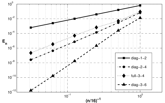
Figure 1: Errors of the SBP-based quadrature rules applied to (20).

4.2 Multi-dimensional Quadrature on a Curvilinear Domain

As shown in Section 3.2, SBP quadrature retains its theoretical accuracy on curvilinear domains provided the Jacobian of the transformation is approximated using the corresponding SBP difference operator. To verify this, we consider the domain

$$\Omega_{x} =\{(x,y)\in\mathbb{R}^{2}\mid 1\leq xy\leq 3,1\leq x^{2}-y^{2}\leq 4\},$$

and the integral

$$\mathcal{I} =\iint\limits_{\Omega_{x}}(x^{2}+y^{2})e^{\frac{1-x^{2}+y^{2}}{3}}\sin{\left(\frac{xy-1}{2}\right)}\,dxdy$$

$$=3(1-e^{-1})(1-\cos(1)).$$ (22)

To compute this integral numerically, we introduce a computational domain based on the coordinates

$$\xi=\frac{x^{2}-y^{2}-1}{3},\qquad\text{and}\quad\eta=\frac{xy-1}{2}.$$

For a given $n\in\{16,32,64,128,256,512\}$, we divide $\xi$ and $\eta$ uniformly into $n+1$ points to produce a Cartesian grid on the square $\Omega_{\xi}=[0,1]^{2}$. The physical coordinates $x$ and $y$ are evaluated at each computational coordinate, and these are used to compute the integrand in (22), which we denote by $f$. The grid for $n=32$ is shown in Figure 2.

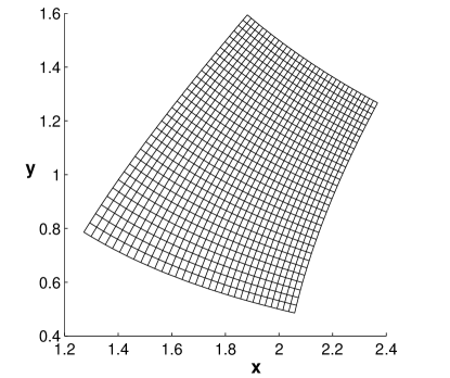
Figure 2: Example grid for $\Omega_{x}$ with $n=32$.

The Jacobian of the transformation is approximated using

$$J=\left[(I\otimes D)x\right]\circ\left[(D\otimes I)y\right]-\left[(I\otimes D)y\right]\circ\left[(D\otimes I)x\right],$$ (23)

where $\circ$ denotes the Hadamard product (the entry-wise product, analogous to matrix addition). We have assumed that the nodes are ordered first by $\xi$ and then by $\eta$, so we can construct the two-dimensional derivative operators using Kronecker products of the one-dimensional operator $D$ and identity matrix $I$.

For a given $n$, the SBP-based approximation of (22) is given by

$$\mathcal{I}_{n}=J^{T}(H\otimes H)f,$$ (24)

and the error in the quadrature is $E_{n}=\mathcal{I}-\mathcal{I}_{n}$. As before, the order of convergence for $n>16$ is estimated by $q_{n}$ given by (21). Figure 3 plots $E_{n}$ and Table 3 lists $q_{n}$ for the diagonal-norm SBP operators listed in Table 1. We focus on the diagonal-norm SBP operators here, because their accuracy is less obvious; the derivatives used to approximate the Jacobian are only $s$-order accurate at the boundary. Nevertheless, as predicted by the theory, Table 3 shows that the quadrature for these schemes remains $2s$-order accurate. Note that the errors for the diag-3-6 scheme are corrupted by round-off error for $n=256$ and $n=512$, which explains the suboptimal values of $q_{n}$ for these grids.

We have also included results for a mixed scheme in Table 3 and Figure 3. This mixed scheme uses the diag-3-6 SBP operator to evaluate the derivatives in the Jacobian (23) and the diag-2-4 operator to evaluate the quadrature (24). The results show that the mixed scheme has an asymptotic convergence rate of only 3. Thus, despite a more accurate approximation of the Jacobian, the mixed scheme produces a less accurate $\mathcal{I}_{n}$ than the scheme using the diag-2-4 operator for both the Jacobian and quadrature. This illustrates the importance of using the same operator to obtain the theoretical convergence rate.

Table 3: Rates of convergence for the diagonal-norm SBP operator approximation of (22).

	$\mathbf{n}$
SBP operator	32	64	128	256	512
diag-1-2	2.0911	2.0453	2.0226	2.0113	-2.0056
diag-2-4	4.3283	4.1583	4.0768	4.0374	-4.0093
diag-3-6	7.0799	6.7941	6.2253	2.1274	-0.7390
mixed	3.3170	2.0521	2.7215	2.8863	- 2.9484

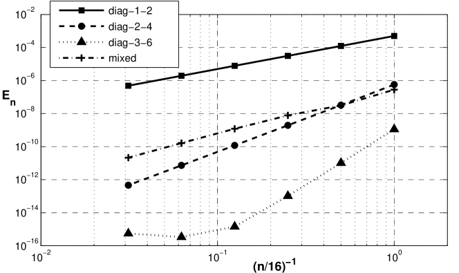
Figure 3: Errors of the SBP-based quadrature rules in approximating (22).

4.3 Discrete Divergence Theorem

In this final example, we verify that SBP operators mimic the divergence theorem accurately. Specifically, we wish to show that when the divergence of a vector field is discretized using SBP operators and then integrated using the corresponding SBP quadrature rule, the result depends only on the nodes along the boundary and is a $2s$-order approximation to the surface flux.

We adopt the same domain $\Omega_{x}$ and coordinate transformation as in the previous example. A vector field $(\mathcal{F},\mathcal{G})$ is defined by

$$\mathcal{F}(x,y) =\phantom{-}\frac{x}{2}\exp{\left(\frac{1-xy}{2}\right)}\cos{\left(\frac{2\pi(x^{2}-y^{2}-1)}{3}\right)}+\frac{2y}{3}\left(\frac{xy-1}{2}\right)^{7}\sin{\left(\frac{\pi(x^{2}-y^{2}-1)}{3}\right)}$$

$$\mathcal{G}(x,y) =-\frac{y}{2}\exp{\left(\frac{1-xy}{2}\right)}\cos{\left(\frac{2\pi(x^{2}-y^{2}-1)}{3}\right)}+\frac{2x}{3}\left(\frac{xy-1}{2}\right)^{7}\sin{\left(\frac{\pi(x^{2}-y^{2}-1)}{3}\right)}.$$

The analytical value of the divergence of $(\mathcal{F},\mathcal{G})$ integrated over the domain $\Omega_{x}$ is

$$\mathcal{I}=\iint\limits_{\Omega_{x}}\frac{\partial\mathcal{F}}{\partial x}+\frac{\partial\mathcal{G}}{\partial y}\,dxdy=\frac{2}{\pi}.$$ (25)

The discrete divergence is evaluated in computational space using approximations for $\hat{\mathcal{F}}$ and $\hat{\mathcal{G}}$. In particular, the derivatives of the spatial coordinates that appear in (16) and (17) are approximated using SBP operators. Therefore, at the nodes, $\hat{\mathcal{F}}$ and $\hat{\mathcal{G}}$ take on the values

$$\hat{f} =\phantom{-}\left[(D\otimes I)y\right]\circ f-\left[(D\otimes I)x\right]\circ g,$$

$$\hat{g} =-\left[(I\otimes D)y\right]\circ f+\left[(I\otimes D)x\right]\circ g,$$

where $f$ and $g$ denote the values of $\mathcal{F}$ and $\mathcal{G}$ evaluated at the nodes.

The SBP approximation of $\mathcal{I}$ is given by (see (15))

$$\mathcal{I}_{n}=c^{T}(H\otimes H)\left[(I\otimes D)\hat{f}+(D\otimes I)\hat{g}\right].$$

Table 4 lists the estimated order of accuracy $q_{n}$ based on $E_{n}=\mathcal{I}-\mathcal{I}_{n}$ for the three diagonal-norm SBP operators diag-1-2, diag-2-4, and diag-3-6. As predicted, the SBP discrete divergence integrated using $(H\otimes H)$ is a $2s$-order accurate approximation to $\mathcal{I}$. Moreover, in light of (19), we know that $\mathcal{I}_{n}$ depends only on the boundary nodes (This has been confirmed by calculating the right-hand side of (19) and showing that it equals $\mathcal{I}_{n}$ to machine error).

Table 4: Rates of convergence for the diagonal-norm SBP operator approximation of an integrated divergence field. Round-off errors are contaminating the estimates for diag-3-6 with $n=256$ and $n=512$

	$\mathbf{n}$
SBP operator	32	64	128	256	512
diag-1-2	2.0909	2.0453	2.0226	2.0113	-2.0056
diag-2-4	3.7201	3.7862	3.9000	3.9532	-3.9758
diag-3-6	7.5935	7.2371	7.8361	5.0507	-2.1760

5 Discussion and Conclusions

We have shown that the weight matrices of SBP finite-difference operators are related to trapezoid rules with end corrections. We make no claim regarding the optimality of these SBP quadrature rules with respect to existing schemes on uniformly spaced grid points. However, the result has significant implications for SBP discretizations of PDEs, which we list below.

• The SBP energy norm, which is frequently used in the stability analysis of SBP-based PDE discretizations, is a $\text{O}(h^{2s})$ accurate approximation of the $L^{2}$ norm for functions on $[0,1]$.

• The summation-by-parts property, equation (1), is a formal and accurate representation of integration by parts, equation (2). More generally, multi-dimensional SBP discretizations using Kronecker products mimic the divergence theorem, i.e. the weight-matrix quadrature applied to the discrete divergence produces an accurate quadrature of the flux over the domain boundary in which no interior points are involved.

• Diagonal-norm SBP operators have $s$ order-accurate boundary closures when the interior scheme is $2s$-order accurate. This limits numerical PDE solutions to $s+1$ order accuracy [11]; however, in [13] we show that a dual consistent SBP discretization leads to super-convergent $2s$-order-accurate functionals, if the corresponding SBP quadrature rule is used to calculate the functional (see also [12]).

In light of these observations, the SBP weight matrix appears to be the natural quadrature rule for evaluating functionals from corresponding SBP discretizations.

Other than its asymptotic form, the leading error term for SBP-based quadrature remains unknown, so we cannot make general statements regarding the relative accuracy of different weight matrices. Although not pursued here, characterizing the leading error term should be possible by finding the finite-difference schemes corresponding to the $\delta_{v}^{(k-1)}$ in Theorem 1.

References

- [1] H.-O. Kreiss, G. Scherer, Finite element and finite difference methods for hyperbolic partial differential equations, in: C. de Boor (Ed.), Mathematical Aspects of Finite Elements in Partial Differential Equations, Mathematics Research Center, the University of Wisconsin, Academic Press, 1974.
- [2] K. Mattsson, M. Svärd, J. Nordström, Stable and accurate artificial dissipation, Journal of Scientific Computing 21 (1) (2004) 57–79.
- [3] J. E. Hicken, D. W. Zingg, A parallel Newton-Krylov solver for the Euler equations discretized using simultaneous approximation terms, AIAA Journal 46 (11) (2008) 2773–2786. doi:10.2514/1.34810.
- [4] K. Mattsson, M. Svärd, M. Shoeybi, Stable and accurate schemes for the compressible navier-stokes equations, Journal of Computational Physics 227 (4) (2008) 2293–2316. doi:10.1016/j.jcp.2007.10.018.
- [5] J. Nordström, J. Gong, E. van der Weide, M. Svärd, A stable and conservative high order multi-block method for the compressible Navier-Stokes equations, Journal of Computational Physics 228 (24) (2009) 9020–9035. doi:10.1016/j.jcp.2009.09.005.
- [6] M. Osusky, J. E. Hicken, D. W. Zingg, A parallel Newton-Krylov-Schur flow solver for the Navier-Stokes equations using the SBP-SAT approach, in: 48th AIAA Aerospace Sciences Meeting, no. AIAA–2010–0116, Orlando, Florida, 2010.
-
[7]
E. Pazos, M. Tiglio, M. D. Duez, L. E. Kidder, S. A. Teukolsky,
Orbiting binary black
hole evolutions with a multipatch high order finite-difference approach,
Physical Review D (Particles, Fields, Gravitation, and Cosmology) 80 (2)
(2009) 024027–1–024027–8.
doi:10.1103/PhysRevD.80.024027.
URL http://link.aps.org/abstract/PRD/v80/e024027 - [8] B. Strand, Summation by parts for finite difference approximations for d/dx, Journal of Computational Physics 110 (1) (1994) 47–67. doi:10.1006/jcph.1994.1005.
- [9] J. Li, General explicit difference formulas for numerical differentiation, Journal of Computational and Applied Mathematics 183 (1) (2005) 29–52. doi:10.1016/j.cam.2004.12.026.
- [10] M. Svärd, On coordinate transformations for summation-by-parts operators, Journal of Scientific Computing 20 (1) (2004) 29–42.
- [11] B. Gustafsson, The convergence rate for difference approximations to mixed initial boundary value problems, Mathematics of Computation 29 (130) (1975) 396–406.
- [12] J. E. Hicken, D. W. Zingg, Superconvergent functional estimates and summation-by-parts finite-difference methods, in: 18th Annual Conference of the CFD Society of Canada, London, Ontario, Canada, 2010.
- [13] J. E. Hicken, D. W. Zingg, Superconvergent functional estimates from summation-by-parts finite-difference discretizations, SIAM Journal on Scientific Computing (accepted) 28.
- [14] F. B. Hildebrand, Introduction to Numerical Analysis, 2nd Edition, McGraw-Hill Inc., New York, NY, 1974.
- [15] T. H. Pulliam, J. L. Steger, Implicit finite-difference simulations of three-dimensional compressible flow, AIAA Journal 18 (2) (1980) 159–167.
- [16] P. D. Thomas, C. K. Lombard, Geometric conservation law and its application to flow computations on moving grids, AIAA Journal 17 (10) (1979) 1030–1037.
- [17] P. Diener, E. N. Dorband, E. Schnetter, M. Tiglio, Optimized high-order derivative and dissipation operators satisfying summation by parts, and applications in three-dimensional multi-block evolutions, Journal of Scientific Computing 32 (1) (2007) 109–145. doi:10.1007/s10915-006-9123-7.