Single-Particle Momentum Distribution of an Efimov trimer

Abstract

Experimental progress in the study of strongly interacting ultracold atoms has recently allowed the observation of Efimov trimers. We study theoretically a non-conventional observable for these trimer states, that may be accessed experimentally, the momentum distribution $n(\mathbf{k})$ of the constitutive bosonic particles. The large momentum part of the distribution is particularly intriguing: In addition to the expected $1/k^{4}$ tail associated to contact interactions, it exhibits a subleading tail $1/k^{5}$ which is a hall-mark of Efimov physics and leads to a breakdown of a previously proposed expression of the energy as a functional of the momentum distribution.

I Introduction

Experiments with ultracold atoms have now entered the regime of strong interactions, thanks to the possibility to manipulate the $s$-wave scattering length $a$ between cold atoms with a magnetically induced Feshbach resonance Feshbach ; revueStringariFermions . This has led to a revolution in the study of the few-body problem, as one can now have in a controllable way a scattering length much larger (in absolute value) than the range $b$ (and the effective range) of the interaction potential. In particular, this has allowed to confirm experimentally Efimov_manips ; Jochim the existence of the long-searched Efimov effect BH ; Efimov1 ; Efimov2 : As shown by Efimov in the early 1970’s, three particles interacting via a short range potential with an infinite scattering length may exhibit an infinite number of trimer states with a geometric spectrum. The existence of an infinite number of bound states is usual, even at the two-body level, for long range interactions, but it is quite intriguing for short range interaction potentials. This Efimov effect takes place for three (same spin state) bosons Efimov1 , but it is more general, it also occurs for example for two (same spin state) fermions and a third distinguishable particle at least $13.607$ times lighter Efimov2 ; PetrovEfim .

On the experimental side, an increasing number of observable quantities are now at hand. For Efimov physics, the usual evidence of the emergence of an Efimov trimer state is a peak in the three-body loss rate as a function of the scattering length Efimov_manips . Now radio-frequency spectroscopic techniques can give a direct access to the trimer spectrum Jochim . For strongly interacting Fermi gases (without Efimov effect) a very precise measurement of the atomic momentum distribution $n(\mathbf{k})$ was performed recently, so precise that it allowed to see the large momentum tail $n(\mathbf{k})\sim C/k^{4}$, $k$ large but still smaller than $1/b$, and to quantitatively extract the coefficient $C$ whose values were satisfactorily compared to theory Jin_nk . The same conclusion holds for the few-body numerical experiment of Blume . Similarly, the first order coherence function $g^{(1)}$ of the atomic field over a distance $r$, a quantity measured for bosonic cold atoms Esslinger but not yet for fermionic cold atoms, is related to the Fourier transform of $n(\mathbf{k})$ and is sensitive to the $1/k^{4}$ tail by a contribution that is non-differentiable with respect to the vector $\mathbf{r}$ in $\mathbf{r}=\mathbf{0}$ lien_g1 , and that appeared in the many-body numerical experiment of Astra .

The occurrence of the $1/k^{4}$ tail in $n(\mathbf{k})$ is a direct consequence of two-body physics, that is of the binary zero-range interaction between two particles, and it holds in all spatial dimensions: According to Schrödinger’s equation for the zero-energy scattering state $\phi(\mathbf{r})$ of two particles of relative coordinates $\mathbf{r}$, $\Delta_{\mathbf{r}}\phi(\mathbf{r})\propto\delta(\mathbf{r})$ for a contact (regularized Dirac delta) interaction contact_interaction , so that in Fourier space $\tilde{\phi}(\mathbf{k})\propto 1/k^{2}$ and $n(\mathbf{k})\propto|\tilde{\phi}(\mathbf{k})|^{2}$ scales as $1/k^{4}$. On the contrary, the coefficient $C$, called contact, depends on the many-body properties, and can be related to the derivative of the gas mean energy (or mean free energy at non-zero temperature) with respect to the scattering length, as was shown first for bosons in one dimension Olshanii , then for spin 1/2 fermions in three dimensions Tan1 ; Braaten_contact ; Tarruell , and for bosonic or fermionic, three dimensional or bidimensional systems, in tangen .

In this paper, we anticipate that experimentally, it may be possible to measure with high precision the atomic momentum distribution in systems subjected to the Efimov effect, for example in a Bose gas with a large scattering length HammerBosons ; Cornell_Bose ; Hulet ; Chevy . To be specific, we consider in the center of mass frame the Efimov trimer states for three bosons interacting with infinite scattering length. After recalling the expression of the three-body wavefunction in section II, we obtain the expression of the momentum distribution in terms of integrals over a single momentum vector in section III, see Eqs.(18,19,20,21,III). As illustrated in section IV, this allows to perform a very precise numerical evaluation of the momentum distribution for all values of the single-particle wavevector $\mathbf{k}$, and to analytically obtain the large momentum behavior of $n(\mathbf{k})$: In addition to the expected $C/k^{4}$ term at large $k$, we find an unexpected $1/k^{5}$ subleading term, that is a direct and generic signature of Efimov physics cluster_Tan , see (26). Another, more formal, consequence of this $1/k^{5}$ subleading term is that the general expression giving the energy as a functional of the momentum distribution $n(\mathbf{k})$, derived for the non-Efimovian case in Tan2 and extended (with the same form) to the Efimovian case in Leyronas , turns out to be invalid in the Efimovian case note2D . We conclude in section V.

II Normalized wavefunction of an Efimov trimer

II.1 Three-body state in position space

In this subsection we recall the wavefunction of an Efimov trimer and give the expression of its normalization constant. We consider an Efimov trimer state for three same-spin-state bosons of mass $m$ interacting via a zero range potential with infinite scattering length. In order to avoid formal normalisability problems, it is convenient to imagine that the Efimov trimer is trapped in an arbitrarily weak harmonic potential, that is with a ground state harmonic oscillator length $a_{\rm ho}$ arbitrarily larger than the trimer size general . Since the center of mass of the system is separable in a harmonic potential, this fixes the normalisability problem without affecting the internal wavefunction of the trimer in the limit $a_{\rm ho}\to+\infty$. In this limit, the energy of the trimer is equal to the free space energy

$$E_{\rm trim}=-\frac{\hbar^{2}\kappa_{0}^{2}}{m},\ \ \ \kappa_{0}>0.$$ (1)

According to Efimov’s asymptotic, zero-range theory Efimov1 ,

$$\kappa_{0}=\frac{\sqrt{2}}{R_{t}}e^{-\pi q/|s_{0}|}e^{\mbox{\scriptsize Arg}\,\Gamma(1+s_{0})/|s_{0}|}$$ (2)

where $R_{t}>0$ is a length known as the three-body parameter def_Rt , the quantum number $q$ is any integer in $\mathbb{Z}$, and the purely imaginary number $s_{0}=i|s_{0}|$ is such that

$$|s_{0}|\cosh(\frac{|s_{0}|\pi}{2})=\frac{8}{\sqrt{3}}\sinh(\frac{|s_{0}|\pi}{6}),$$ (3)

so that $|s_{0}|=1.00623782510\ldots$ The corresponding three-body wavefunction $\Psi$ may be written for $\kappa_{0}a_{\rm ho}\to+\infty$ as

$$\Psi(\mathbf{r}_{1},\mathbf{r}_{2},\mathbf{r}_{3})=\psi_{\rm CM}(\mathbf{C})\left[\psi(r_{12},\frac{|2\mathbf{r}_{3}-(\mathbf{r}_{1}+\mathbf{r}_{2})|}{\sqrt{3}})\right.\\ \left.+\psi(r_{23},\frac{|2\mathbf{r}_{1}-(\mathbf{r}_{2}+\mathbf{r}_{3})|}{\sqrt{3}})+\psi(r_{31},\frac{|2\mathbf{r}_{2}-(\mathbf{r}_{3}+\mathbf{r}_{1})|}{\sqrt{3}})\right],$$ (4)

where $\mathbf{C}=(\mathbf{r}_{1}+\mathbf{r}_{2}+\mathbf{r}_{3})/3$ is the center of mass position of the three particles and the parameterization of $\psi$ is related to the Jacobi coordinates $\mathbf{r}=\mathbf{r}_{2}-\mathbf{r}_{1}$ and $\mbox{\boldmath$\rho$}=[2\mathbf{r}_{3}-(\mathbf{r}_{1}+\mathbf{r}_{2})]/\sqrt{3}$. In our expression of $\Psi$, $\psi_{\rm CM}$ is the Gaussian wavefunction of the center of mass ground state in the harmonic trap, normalized to unity, and $\psi$ is a Faddeev component of the free space trimer wavefunction. The explicit expression of $\psi$ is known Efimov1 :

$$\psi(r,\rho)=\frac{\mathcal{N}_{\psi}}{\sqrt{4\pi}}\frac{K_{s_{0}}(\kappa_{0}\sqrt{r^{2}+\rho^{2}})}{(r^{2}+\rho^{2})/2}\frac{\sin[s_{0}(\frac{\pi}{2}-\alpha)]}{\sin(2\alpha)}$$ (5)

where $K_{s_{0}}$ is a Bessel function and $\alpha=\mbox{atan}(r/\rho)$. The normalization factor $\mathcal{N}_{\psi}$ ensuring that $||\Psi||^{2}=1$ was not calculated in Efimov1 . To obtain its explicit expression, one first performs the change of variables $(\mathbf{r}_{1},\mathbf{r}_{2},\mathbf{r}_{3})\to(\mathbf{C},\mbox{\boldmath$\rho$},\mathbf{r})$, whose Jacobian is $D(\mathbf{r}_{1},\mathbf{r}_{2},\mathbf{r}_{3})/D(\mathbf{C},\mbox{\boldmath$\rho$},\mathbf{r})=(-\sqrt{3}/2)^{3}$. To integrate over $\mathbf{r}$ and $\rho$ one then introduces hyperspherical coordinates in which the wavefunction separates; one then faces known integrals on the hyperradius Gradstein and on the hyperangles Efimov93 . This leads to WernerThese :

$$|\mathcal{N}_{\psi}|^{-2}=\left(\frac{\sqrt{3}}{2}\right)^{3}\frac{3\pi^{2}}{2\kappa_{0}^{2}\cosh(\frac{|s_{0}|\pi}{2})}\\ \times\left[\cosh(\frac{|s_{0}|\pi}{2})+\frac{|s_{0}|\pi}{2}\sinh(\frac{|s_{0}|\pi}{2})-\frac{4\pi}{3\sqrt{3}}\cosh(\frac{|s_{0}|\pi}{6})\right].$$ (6)

II.2 Three-body state in momentum space

To obtain the momentum distribution for the Efimov trimer, we need to evaluate the Fourier transform of the trimer wavefunction $\Psi$ given by (4). Rather than directly using (5), we take advantage of the fact that, for contact interactions, the Faddeev component $\psi$ obeys the non-interacting Schrödinger’s equation with a source term. With the change to Jacobi coordinates, the Laplace operator in the coordinate space of dimension nine reads $\sum_{i=1}^{3}\Delta_{\mathbf{r}_{i}}=\frac{1}{3}\Delta_{\mathbf{C}}+2\left[\Delta_{\mathbf{r}}+\Delta_{\mbox{\boldmath$\rho$}}\right]$ so that

$$-\left[\kappa_{0}^{2}-\Delta_{\mathbf{r}}-\Delta_{\mbox{\scriptsize\boldmath$\rho$}}\right]\psi(r,\rho)=\delta(\mathbf{r})B(\rho).$$ (7)

The source term in the right hand side originates from the fact that

$$\psi(r,\rho)\underset{r\to 0}{\sim}-\frac{B(\rho)}{4\pi r}$$ (8)

for a fixed $\rho$, this $1/r$ divergence coming from the replacement of the interaction potential by the Bethe-Peierls contact condition. Taking the Fourier transform of (7) over $\mathbf{r}$ and $\rho$ leads to

$$\tilde{\psi}(k,K)=-\frac{\tilde{B}(K)}{k^{2}+K^{2}+\kappa_{0}^{2}},$$ (9)

where the Fourier transform is defined as $\tilde{B}(K)\equiv\int d^{3}\rho\,e^{-i\mathbf{K}\cdot\mbox{\scriptsize\boldmath$\rho$}}B(\rho)$. $B(\rho)$ is readily obtained from (5) by taking the limit $r\to 0$:

$$B(\rho)=-\mathcal{N}_{\psi}(4\pi)^{1/2}i\sinh(\frac{|s_{0}|\pi}{2})\frac{K_{s_{0}}(\kappa_{0}\rho)}{\rho}.$$ (10)

The Fourier transform of this expression is known, see relation 6.671(5) in Gradstein , so that

$$\!\!\!\!\!\!\tilde{B}(K)=\frac{-2\pi^{5/2}\mathcal{N}_{\psi}}{K(K^{2}+\kappa_{0}^{2})^{1/2}}\left\{\left[\frac{(K^{2}+\kappa_{0}^{2})^{1/2}+K}{\kappa_{0}}\right]^{s_{0}}\!\!\!\!-\mbox{c.c.}\right\}$$ (11)

where c.c. stands for the complex conjugate. Note that the expression between the curly brackets simply reduces to $2i\sin(|s_{0}|\alpha)$ if one sets $K=\kappa_{0}\sinh\alpha$. What we shall need is the large $K$ behavior of $\tilde{B}(K)$. Expanding (11) in powers of $\kappa_{0}/K$ gives

$$\tilde{B}(K)=\mathcal{N}_{\psi}\frac{2\pi^{5/2}}{K^{2}}\left[(2K/\kappa_{0})^{-s_{0}}-\mbox{c.c.}\right]+O(1/K^{4}).$$ (12)

The last step to obtain the trimer state vector in momentum space is to take the Fourier transform of (4), using the appropriate Jacobi coordinates for each Faddeev component, or simply by Fourier transforming the first Faddeev component using the coordinates $(\mathbf{C},\mathbf{r},\mbox{\boldmath$\rho$})$ given above and by performing circular permutations on the particle labels. This gives

$$\tilde{\Psi}(\mathbf{k}_{1},\mathbf{k}_{2},\mathbf{k}_{3})=\left(\frac{\sqrt{3}}{2}\right)^{3}\tilde{\psi}_{\rm CM}(\mathbf{k}_{1}+\mathbf{k}_{2}+\mathbf{k}_{3})\\ \times\Big{[}\tilde{\psi}\left(\frac{|\mathbf{k}_{2}-\mathbf{k}_{1}|}{2},\frac{|2\mathbf{k}_{3}-(\mathbf{k}_{1}+\mathbf{k}_{2})|}{2\sqrt{3}}\right)+(231)+(312)\Big{]},$$ (13)

where the notation $(ijk)$ means that the indices $1,2,3$ have been replaced by $i,j,k$ respectively.

III Integral expression of the momentum distribution

To obtain the momentum distribution for an Efimov trimer state, it remains to integrate over $\mathbf{k}_{3}$ and $\mathbf{k}_{2}$ the modulus square of the Fourier transform (13) of the trimer wavefunction. In the limit $\kappa_{0}a_{\rm ho}\to+\infty$ where one suppresses the harmonic trapping, one can set

$$|\tilde{\psi}_{\rm CM}(\mathbf{k}_{1}+\mathbf{k}_{2}+\mathbf{k}_{3})|^{2}=(2\pi)^{3}\delta(\mathbf{k}_{1}+\mathbf{k}_{2}+\mathbf{k}_{3})$$ (14)

so that the trimer is at rest in all what follows. Integration over $\mathbf{k}_{3}$ is then straightforward:

$$n(\mathbf{k}_{1})=3\left(\frac{\sqrt{3}}{2}\right)^{6}\int\frac{d^{3}k_{2}}{(2\pi)^{3}}\Big{|}\tilde{\psi}(\frac{|\mathbf{k}_{2}-\mathbf{k}_{1}|}{2},\frac{\sqrt{3}|\mathbf{k}_{1}+\mathbf{k}_{2}|}{2})\\ +\tilde{\psi}(|\mathbf{k}_{2}+\frac{1}{2}\mathbf{k}_{1}|,\frac{\sqrt{3}}{2}k_{1})+\tilde{\psi}(|\mathbf{k}_{1}+\frac{1}{2}\mathbf{k}_{2}|,\frac{\sqrt{3}}{2}k_{2})\Big{|}^{2}.$$ (15)

The factor $3$ in the right hand side results from the fact that, as e.g. in Tan1 , we normalize the momentum distribution $n(\mathbf{k})$ to the total number of particles (rather than to unity):

$$\int\frac{d^{3}k}{(2\pi)^{3}}\,n(\mathbf{k})=3.$$ (16)

Also note that the sum of the squares of the arguments of $\tilde{\psi}$ is constant and equal to $k_{1}^{2}+k_{2}^{2}+\mathbf{k}_{1}\cdot\mathbf{k}_{2}$ for each term in the right hand side of (15). When using (9), one can thus put the denominator in (9) as a common denominator, to obtain

$$\!\!\!\!\!\!n(\mathbf{k}_{1})=\!\!\int\!\!\frac{d^{3}k_{2}}{(2\pi)^{3}}\frac{\left[\tilde{B}(\frac{\sqrt{3}}{2}|\mathbf{k}_{1}+\mathbf{k}_{2}|)+\tilde{B}(\frac{\sqrt{3}}{2}k_{1})+\tilde{B}(\frac{\sqrt{3}}{2}k_{2})\right]^{2}}{(4^{3}/3^{4})(k_{1}^{2}+k_{2}^{2}+\mathbf{k}_{1}\cdot\mathbf{k}_{2}+\kappa_{0}^{2})^{2}}.$$ (17)

For simplicity, we have assumed that the normalization factor $\mathcal{N}_{\psi}$ is purely imaginary, so that $\tilde{B}(K)$ is a real quantity.

In the above writing of $n(\mathbf{k}_{1})$, the only “nasty” contribution is $\tilde{B}(\sqrt{3}|\mathbf{k}_{1}+\mathbf{k}_{2}|/2)$; the other contributions are “nice” since they only depend on the moduli $k_{1}$ and $k_{2}$. Expanding the square in the numerator of (17), one gets six terms, three squared terms and three crossed terms. The change of variable $\mathbf{k}_{2}=-(\mathbf{k}^{\prime}_{2}+\mathbf{k}_{1})$ allows, in one of the squared terms and in one of the crossed terms, to transform a nasty term into a nice term. What remains is a nasty crossed term that cannot be turned into a nice one; in that term, as a compromise, one performs the change of variable $\mathbf{k}_{2}=-(\mathbf{k}_{2}^{\prime}+\mathbf{k}_{1}/2)$. We finally obtain the momentum distribution as the sum of four contributions,

$$n(\mathbf{k}_{1})=n_{\rm I}(\mathbf{k}_{1})+n_{\rm II}(\mathbf{k}_{1})+n_{\rm III}(\mathbf{k}_{1})+n_{\rm IV}(\mathbf{k}_{1}),$$ (18)

with

$$n_{\rm I}(\mathbf{k}_{1}) \!\!\!=\!\! \frac{3^{4}}{4^{3}}\!\!\int\!\!\frac{d^{3}k_{2}}{(2\pi)^{3}}\frac{\tilde{B}^{2}(\frac{\sqrt{3}}{2}k_{1})}{(k_{1}^{2}+k_{2}^{2}+\mathbf{k}_{1}\cdot\mathbf{k}_{2}+\kappa_{0}^{2})^{2}}$$ (19)

$$n_{\rm II}(\mathbf{k}_{1}) \!\!\!=\!\! \frac{3^{4}}{4^{3}}\!\!\int\!\!\frac{d^{3}k_{2}}{(2\pi)^{3}}\frac{2\tilde{B}^{2}(\frac{\sqrt{3}}{2}k_{2})}{(k_{1}^{2}+k_{2}^{2}+\mathbf{k}_{1}\cdot\mathbf{k}_{2}+\kappa_{0}^{2})^{2}}$$ (20)

$$n_{\rm III}(\mathbf{k}_{1}) \!\!\!=\!\! \frac{3^{4}}{4^{3}}\!\!\int\!\!\frac{d^{3}k_{2}}{(2\pi)^{3}}\frac{4\tilde{B}(\frac{\sqrt{3}}{2}k_{1})\tilde{B}(\frac{\sqrt{3}}{2}k_{2})}{(k_{1}^{2}+k_{2}^{2}+\mathbf{k}_{1}\cdot\mathbf{k}_{2}+\kappa_{0}^{2})^{2}}$$ (21)

$$n_{\rm IV}(\mathbf{k}_{1}) \!\!\!=\!\! \frac{3^{4}}{4^{3}}\!\!\int\!\!\frac{d^{3}k_{2}}{(2\pi)^{3}}\frac{2\tilde{B}(\frac{\sqrt{3}}{4}|2\mathbf{k}_{2}+\mathbf{k}_{1}|)\tilde{B}(\frac{\sqrt{3}}{4}|2\mathbf{k}_{2}-\mathbf{k}_{1}|)}{(\kappa_{0}^{2}+k_{2}^{2}+\frac{3}{4}k_{1}^{2})^{2}}.$$

An interesting question is to know if one can go beyond the integral expressions Eqs.(19,20,21,III), that is if one can obtain an explicit expression for the momentum distribution, at most in terms of special functions. The contribution $n_{\rm I}(\mathbf{k}_{1})$ is straightforward to calculate:

$$n_{\rm I}(\mathbf{k}_{1})=\frac{\sqrt{3}}{4\pi}\left(\frac{3}{4}\right)^{3}\frac{\tilde{B}^{2}(\sqrt{3}k_{1}/2)}{(k_{1}^{2}+4\kappa_{0}^{2}/3)^{1/2}}.$$ (23)

The contribution $n_{\rm II}(\mathbf{k}_{1})$ is also explicitly calculable by performing the change of variable $k_{2}=(2/\sqrt{3})\kappa_{0}\sinh\alpha$ and using the identity that can be derived from contour integration:

$$\int_{-\infty}^{+\infty}d\alpha\,\frac{e^{is\alpha}}{\cosh\alpha-\cosh\alpha_{0}}=\frac{2\pi\sin[s(i\pi-\alpha_{0})]}{\sinh\alpha_{0}\sinh(s\pi)},$$ (24)

where $s$ is any real number and $\alpha_{0}$ is any complex number with $0<\mbox{Im}\,\alpha_{0}<\pi$. This also allows to obtain an explicit expression of $n_{\rm III}(\mathbf{k}_{1})$ if one further applies integration by part, integrating the factor $\sin(|s_{0}|\alpha)$. We do not give however the resulting expressions since, contrarily to these first three contributions to $n(\mathbf{k}_{1})$, the contribution $n_{\rm IV}(\mathbf{k}_{1})$ in (III) blocked our attempt to calculate $n(\mathbf{k}_{1})$ explicitly. For $\mathbf{k}_{1}=\mathbf{0}$ however it becomes equal to the contribution $n_{\rm II}$. $n(\mathbf{k}_{1}=0)$ can thus be evaluated explicitly in terms of $\kappa_{0}$ and $s_{0}$, see Appendix F in tangen . In numerical form this gives

$$n(\mathbf{k}=\mathbf{0})=\frac{55.43379775608\ldots}{\kappa_{0}^{3}}.$$ (25)

IV Applications

IV.1 Numerical evaluation of $n(\mathbf{k})$ at all $k$

The integral expression of $n(\mathbf{k})$ derived in section III allows a straightforward and very precise numerical calculation of the single-particle momentum distribution for an infinite scattering length Efimov trimer, once all the doable angular integrations have been performed in spherical coordinates of polar axis $\mathbf{k}_{1}$. The result is shown for low values of $k$ in Fig.1a, and for high values of $k$ in Fig.1b. In particular, Fig.1b was constructed to show how $n(\mathbf{k})$ approaches the asymptotic behavior (26) derived in the next subsection, that is to reveal the existence of a $1/k^{5}$ sub-leading oscillating term. Note that the accuracy of the numerics may be tested from (25) and from the explicit analytical expressions of $n_{\rm I}$ (given in (23)), of $n_{\rm II}$ and of $n_{\rm III}$ (not given).

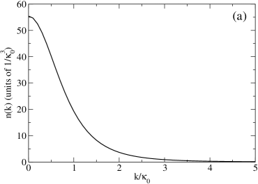
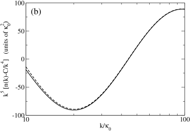
Figure 1: For a free space Efimov trimer at rest composed of three bosonic particles of mass $m$ interacting via a zero-range, infinite scattering length potential, single-particle momentum distribution $n(\mathbf{k})$ as a function of $k$. (a) Numerical calculation from the expression for $n(\mathbf{k})$ appearing in Eq.(18). (b) Numerical calculation (solid line) and asymptotic behavior (26) (dashed line), with the horizontal axis in log scale. The unit of momentum is $\kappa_{0}$, such that the trimer energy is $-\hbar^{2}\kappa_{0}^{2}/m$.

IV.2 Large momentum behavior of $n(\mathbf{k})$

Starting from the integral representation Eqs.(19,20,21,III), we show in the Appendix A that the single-particle momentum distribution has the asymptotic expansion at large wavevectors:

$$n(\mathbf{k})\underset{k\to\infty}{=}\frac{C}{k^{4}}+\frac{D}{k^{5}}\cos\left[2|s_{0}|\ln(\sqrt{3}k/\kappa_{0})+\varphi\right]+\ldots$$ (26)

where we recall that the trimer energy is $E_{\rm trim}=-\hbar^{2}\kappa_{0}^{2}/m$, and the quantities $C$, $D$ and $\varphi$ derived in the Appendix A are given by

$$C/\kappa_{0} = 8\pi^{2}\sinh(|s_{0}|\pi/2)\tanh(|s_{0}|\pi)/\Big{[}\cosh(\frac{|s_{0}|\pi}{2})$$ (27)

$$+\frac{|s_{0}|\pi}{2}\sinh(\frac{|s_{0}|\pi}{2})-\frac{4\pi}{3\sqrt{3}}\cosh(\frac{|s_{0}|\pi}{6})\Big{]}$$

$$= 53.09722846003081\ldots$$ (28)

$$D/\kappa_{0}^{2} \simeq -89.26260$$ (29)

$$\varphi \simeq -0.8727976.$$ (30)

The crucial point is that $D\neq 0$: Due to the Efimov effect, the momentum distribution has a slowly decaying $O(1/k^{5})$ oscillatory subleading tail.

IV.3 Breakdown of the usual energy-momentum distribution relation

In Leyronas it was proposed that the expression of the energy as a functional of the momentum distribution, derived in Tan2 for equal mass spin 1/2 fermions, also holds for bosons (apart from the appropriate change of numerical factors). In the present case of a free space Efimov trimer at rest with an infinite scattering length, the energy formula of Leyronas reduces to

$$E_{\rm trim}\stackrel{{\scriptstyle?}}{{=}}\int\frac{d^{3}k}{(2\pi)^{3}}\frac{\hbar^{2}k^{2}}{2m}\Big{[}n(\mathbf{k})-\frac{C}{k^{4}}\Big{]}.$$ (31)

We have however put a question mark, because the asymptotic expansion (26) implies that the integral in (31) is not well-defined: After the change of variables $x=\ln(\sqrt{3}k/\kappa_{0})$, the integrand behaves for $x\to+\infty$ as a linear superposition of $e^{2i|s_{0}|x}$ and $e^{-2i|s_{0}|x}$, that is as a periodic function of $x$ oscillating around zero. This was overlooked in Leyronas .

At first sight, however, this does not look too serious: One often argues, when one faces the integral of such an oscillating function of zero mean, that the oscillations at infinity simply average to zero. More precisely, let us define the cut-off dependent energy functional

$$E(\Lambda)=\int_{k<\Lambda}\frac{d^{3}\!k}{(2\pi)^{3}}\frac{\hbar^{2}k^{2}}{2m}\left[n(\mathbf{k})-\frac{C}{k^{4}}\right],$$ (32)

where the integration is limited to wavevectors $\mathbf{k}$ of modulus less than the cut-off. For $\Lambda\to+\infty$, $E(\Lambda)$ is asymptotically an oscillating function of the logarithm of $\Lambda$, oscillating around a mean value $\bar{E}$. The naive expectation would be that the trimer energy $E_{\rm trim}$ equals $\bar{E}$. This naive expectation is equivalent to the usual trick used to regularize oscillating integrals, consisting here in introducing a convergence factor $e^{-\eta\ln(\sqrt{3}k/\kappa_{0})}$ in the integral without momentum cut-off and then taking the limit $\eta\to 0^{+}$:

$$\lim_{\eta\to 0^{+}}\int_{\mathbb{R}^{3}}\frac{d^{3}\!k}{(2\pi)^{3}}\frac{\hbar^{2}k^{2}}{2m}\left[n(\mathbf{k})-\frac{C}{k^{4}}\right]e^{-\eta\ln(\sqrt{3}k/\kappa_{0})}=\bar{E}.$$ (33)

To test the naive regularization procedure, we performed a numerical calculation of $E(\Lambda)$, using the result (18) to perform a very accurate numerical calculation of $n(\mathbf{k})$. The result is shown as a solid line in Fig.2. We also developed a more direct technique allowing a numerical calculation of $E(\Lambda)$ without the knowledge of $n(\mathbf{k})$, see Appendix B: The corresponding results are represented as $+$ symbols in Fig.2 and are in perfect agreement with the solid line. As expected, $E(\Lambda)$ is asymptotically an oscillating function of the logarithm of $\Lambda$, oscillating around a mean value $\bar{E}$.

To formalize, we introduce an arbitrary, non-zero value $k_{\rm min}$ of the momentum. We define $\delta n(k)=n(\mathbf{k})-C/k^{4}$ for $k<k_{\rm min}$, and for $k>k_{\rm min}$:

$$\delta n(k)=n(\mathbf{k})-\left\{\frac{C}{k^{4}}+\frac{D}{k^{5}}\cos\left[2|s_{0}|\ln(\sqrt{3}k/\kappa_{0})+\varphi\right]\right\}.$$ (34)

The introduction of $k_{\rm min}$ ensures that the integral of $k^{2}\delta n(k)$ over all $\mathbf{k}$ converges around $\mathbf{k}=\mathbf{0}$. The subtraction of the asymptotic behavior of $n(\mathbf{k})$ up to order $O(1/k^{5})$ for $k>k_{\rm min}$ ensures that the integral of $k^{2}\delta n(k)$ over all $\mathbf{k}$ converges at infinity. As a consequence we get in the large cut-off limit

$$E(\Lambda)=\bar{E}+\frac{\hbar^{2}D}{8\pi^{2}m|s_{0}|}\sin[2|s_{0}|\ln(\sqrt{3}\Lambda/\kappa_{0})+\varphi]+O(1/\Lambda),$$ (35)

with

$$\bar{E}=-\frac{\hbar^{2}D}{8\pi^{2}m|s_{0}|}\sin[2|s_{0}|\ln(\sqrt{3}k_{\rm min}/\kappa_{0})+\varphi]\\ +\int_{0}^{+\infty}dk\,\frac{\hbar^{2}k^{4}}{4\pi^{2}m}\delta n(k).$$ (36)

From this last equation (36) and the numerical calculations of $n(\mathbf{k})$ first up to $k=1000\kappa_{0}$ and then up to $k\simeq 5500\kappa_{0}$, we get two slightly different values of $\bar{E}$, which gives an estimate with an error bar astuce :

$$\bar{E}\simeq 0.89397(3)E_{\rm trim}.$$ (37)

The conclusion is that $\bar{E}$ (significantly) differs from $E_{\rm trim}$: The naive regularization of the energy formula proposed in Leyronas does not give the correct value of the trimer energy.

An analytical representation of $\bar{E}$ in terms of single integrals can be obtained, see Appendix C. This analytical calculation gives a physical explanation of the failure of the naive regularization: It is inconsistent to add by hand the regularization factor $e^{-\eta\ln(\sqrt{3}k/\kappa_{0})}$ at the last stage, that is in the integrand of (31). To be consistent, the momentum cut-off function has to be introduced at the level of the three-body problem. Then the subleading $1/k^{5}$ term in the momentum distribution acquires a small non-oscillating component, of order $\eta/k^{5}$, that gives a non-zero contribution to the integral (31) for $\eta\to 0^{+}$, since $\int_{k_{\rm min}}^{+\infty}dk\,k^{4}\frac{\eta}{k^{5}}e^{-\eta\ln(\sqrt{3}k/\kappa_{0})}$ does not tend to zero in this limit. The resulting integral representation of $\bar{E}$ confirms the numerical result and allows to evaluate $\bar{E}$ with a better precision:

$$\bar{E}/E_{\rm trim} = 1-\frac{4\cosh(|s_{0}|\pi/2)}{\pi\sqrt{3}}\Big{[}\cosh(|s_{0}|\pi/2)+\frac{|s_{0}|\pi}{2}\sinh(|s_{0}|\pi/2)-\frac{4\pi}{3\sqrt{3}}\cosh(|s_{0}|\pi/6)\Big{]}^{-1}$$ (38)

$$\times \int_{0}^{+\infty}dq\,\left\{\frac{2\ln(q)\cos(|s_{0}|\ln q)}{1+q^{2}+q^{4}}+\frac{16q\ln[(1+q^{2})/4]}{|s_{0}|(1+q^{2})(q^{2}+3)^{2}}\sin\left(|s_{0}|\ln\frac{1+q}{|1-q|}\right)\right.$$

$$\left.+4\ln\left(\frac{1+q^{2}}{|1-q^{2}|}\right)\cos\left(|s_{0}|\ln\frac{1+q}{|1-q|}\right)\left[\frac{1}{2(q^{2}+3)}+\frac{\ln[2(1+q^{2})/(q^{2}+3)]}{1-q^{2}}\right]\right\}$$

$$= 0.8939667780883\ldots$$ (39)

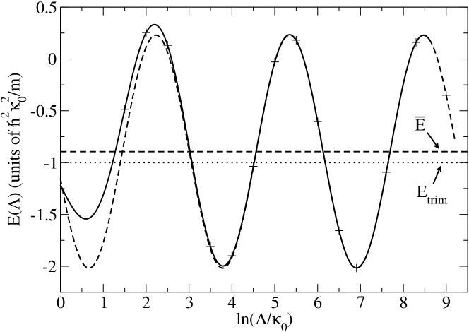
Figure 2: Cut-off dependent energy $E(\Lambda)$ as defined in (32) for a free space infinite scattering length Efimov trimer with a zero-range interaction, as a function of the logarithm of the momentum cut-off $\Lambda$. Solid line: numerical result obtained via a calculation of the momentum distribution $n(\mathbf{k})$. Symbols $+$: direct numerical calculation of $E(\Lambda)$ as exposed in the Appendix B. Dashed sinusoidal line: asymptotic oscillatory behavior of $E(\Lambda)$ for large $\Lambda$, obtained by omitting $O(1/\Lambda)$ in (35). Dashed horizontal line: mean value $\bar{E}$ around which $E(\Lambda)$ oscillates at large $\Lambda$. The values of $\bar{E}$ obtained analytically (38) and numerically (37) are indistinguishable at the scale of the figure, and clearly deviate from the dotted line giving the true energy $E_{\rm trim}$ of the trimer, exemplifying the failure of a at a first sight convincing application of an energy formula for bosons in three dimensions. The unit of momentum $\kappa_{0}$ is such that the true trimer energy is $E_{\rm trim}=-\hbar^{2}\kappa_{0}^{2}/m$.

V Conclusion

We have calculated the single-particle momentum distribution $n(\mathbf{k})$ for the free space Efimov trimer states of same spin state bosons interacting via a zero-range potential with an infinite scattering length. The asymptotic behavior of $n(\mathbf{k})$ at large wavevectors, that we determined with good precision, is of particular interest: In addition to the $C/k^{4}$ tail expected from two-body physics, it has a subleading oscillating $1/k^{5}$ contribution, which is a signature of Efimov physics that one may try to observe experimentally.

We obtained the analytical expression for the coefficient $C$, see (27). This coefficient can also be obtained by a direct calculation in position space, using the fact that $C$ is proportional to $\int d^{3}\rho\,|B(\rho)|^{2}$ WernerThese ; tangen . This result allows to calculate the trimer energy for a finite scattering length $a$, to first order in $1/a$, thanks to the relation tangen

$$\left(\frac{\partial E_{\rm trim}}{\partial(-1/a)}\right)_{R_{t}}=\frac{\hbar^{2}C}{8\pi m}$$ (40)

where the derivative is taken for a fixed value of the three-body parameter $R_{t}$. In other words, we obtained analytically the derivative at $-\pi/2$ of Efimov’s universal function $\Delta(\xi)$ BH . In numerical form, it gives $\Delta^{\prime}(-\pi/2)=2.125850069373\ldots$, which refines the previously known numerical estimate $\simeq 2.12$ BH . Furthermore, the existence of the $1/k^{5}$ subleading term leads to a failure of the relation proposed in Leyronas expressing the energy as a functional of the single-particle momentum distribution, which was not obvious a priori.

We have considered here the particular case of Efimov trimers. The coefficient of the $1/k^{5}$ subleading term was however obtained in Appendix A by taking the zero-energy limit $\kappa_{0}\to 0$. We thus expect that the phenomenology of the $1/k^{5}$ subleading term persists, not only for any other three-body system subjected to Efimov physics (such as two fermions of mass $M$ and a lighter particle of mass $m$ with a mass ratio $M/m>13.607$ Efimov2 ; PetrovEfim ), but also for a macroscopic Bose gas, at least for strong enough interactions Cornell_Bose ; Chevy so as to make the subleading $1/k^{5}$ term sizeable and maybe accessible to measurements. More precisely, we conjectured in tangen that there is a subleading oscillating $1/k^{5}$ term in the tail of the momentum distribution [as in Eq.(26)] for any $N$-body quantum state subjected to the Efimov effect, that is obeying three-body contact conditions involving the three-body parameter $R_{t}$, with a coefficient $D$ related to $\partial E/\partial(\ln R_{t})$ through a simple proportionality factor. Moreover, this derivative was related in tangen to a three-body analog of the contact, defined from the prefactor appearing in the three-body contact condition.

Note: After submission of this work, (i) the expression of the coefficient of the $1/k^{5}$ subleading tail of $n(\mathbf{k})$ in terms of the derivative of the energy with respect to the logarithm of the three-body parameter $R_{t}$, and (ii) the appropriate energy formula taking into account the Efimovian subleading $1/k^{5}$ term, appeared in platter_efim for a Bose gas with an arbitrary number of particles.

Appendix A Leading and next-to-leading terms for $n(\mathbf{k})$ at large momentum

Here we derive the asymptotic expansion (26). We shall take the large $k_{1}$ limit, or equivalently formally the $\kappa_{0}\to 0$ limit for a fixed $k_{1}$. From the asymptotic behavior (12) we see that $\tilde{B}^{2}(k_{1})$ involves a sum of “oscillating” terms involving $k_{1}^{2s_{0}}$ or $k_{1}^{-2s_{0}}$, and of “non-oscillating” terms. We shall calculate first the resulting non-oscillating contribution, then the resulting oscillating one, up to order $1/k_{1}^{5}$ included.

A.0.1 Non-oscillating contribution up to $O(1/k_{1}^{5})$

We consider the small $\kappa_{0}$ limit successively for each of the four components of $n(k_{1})$ in (18).

Contribution I: Taking directly $\kappa_{0}\to 0$ in the integral defining $n_{\rm I}$, replacing $\tilde{B}(k_{1})$ by its asymptotic behavior (12) and averaging out the oscillating terms $k_{1}^{\pm 2s_{0}}$ gives the leading behavior

$$\langle n_{\rm I}(\mathbf{k}_{1})\rangle\simeq\frac{3\sqrt{3}}{8\pi}|\mathcal{N}_{\psi}|^{2}\frac{4\pi^{5}}{k_{1}^{5}}.$$ (41)

Contribution II: In the integrand of (20), we use the splitting

$$(k_{1}^{2}+k_{2}^{2}+\mathbf{k}_{1}\cdot\mathbf{k}_{2}+\kappa_{0}^{2})^{-2}=k_{1}^{-4}\\ +\left[(k_{1}^{2}+k_{2}^{2}+\mathbf{k}_{1}\cdot\mathbf{k}_{2}+\kappa_{0}^{2})^{-2}-k_{1}^{-4}\right].$$ (42)

The first term in the right hand side gives a contribution exactly scaling as $1/k_{1}^{4}$. In the contribution of the second term in the right hand side, one may take the limit $\kappa_{0}\to 0$ and replace $\tilde{B}^{2}(\sqrt{3}k_{2}/2)$ by its asymptotic expression to get the subleading $1/k_{1}^{5}$ contribution. Performing the change of variable $\mathbf{k}_{2}=k_{1}\mathbf{q}$ in the integral and averaging out the oscillating terms $k_{1}^{\pm 2s_{0}}$ gives

$$\langle n_{\rm II}(k_{1})\rangle=\frac{C}{k_{1}^{4}}-\frac{3\sqrt{3}}{2\pi}|\mathcal{N}_{\psi}|^{2}\frac{4\pi^{5}}{k_{1}^{5}}+o(1/k_{1}^{5}),$$ (43)

with

$$C=3(\sqrt{3}/2)^{6}\int\frac{d^{3}k_{2}}{(2\pi)^{3}}2\tilde{B}^{2}(\sqrt{3}k_{2}/2).$$ (44)

We calculate $C$ from the exact expression (11) of $\tilde{B}$: We integrate over solid angles and we use the change of variables $\frac{\sqrt{3}}{2}k_{2}=\kappa_{0}\sinh\alpha$, where $\alpha$ varies from zero to $+\infty$, to take advantage of the fact that

$$\tilde{B}(\kappa_{0}\sinh\alpha)=-\frac{2\pi^{5/2}\mathcal{N}_{\psi}}{\kappa_{0}^{2}\sinh\alpha\cosh\alpha}\left(e^{s_{0}\alpha}-e^{-s_{0}\alpha}\right).$$ (45)

This leads to

$$C=12\pi^{3}(\sqrt{3}/2)^{3}\frac{|\mathcal{N}_{\psi}|^{2}}{\kappa_{0}}\int_{0}^{+\infty}d\alpha\,\frac{2-(e^{2s_{0}\alpha}+\mbox{c.c.})}{\cosh\alpha},$$ (46)

where we used the fact that $\mathcal{N}_{\psi}^{2}=-|\mathcal{N}_{\psi}|^{2}$. The resulting integral over $\alpha$ may be extended over the whole real axis because the integrand is an even function of $\alpha$; it may then be evaluated by using the general result (that we obtained with contour integration)

$$K(\theta,s)\equiv\int_{-\infty}^{+\infty}d\alpha\,\frac{e^{is\alpha}}{\cosh\alpha+\cos\theta}=\frac{2\pi}{\sin\theta}\frac{\sinh(s\theta)}{\sinh(s\pi)}$$ (47)

where $s$ is a real number and $\theta\in]0,\pi[$. One simply has to take $\theta=\pi/2$, $s\to 0$ and $s=2|s_{0}|$ respectively. We get

$$C=\frac{24\pi^{4}}{\kappa_{0}}\left(\frac{\sqrt{3}}{2}\right)^{3}\frac{\sinh^{2}(|s_{0}|\pi/2)}{\cosh(|s_{0}|\pi)}\,|\mathcal{N}_{\psi}|^{2}.$$ (48)

This, together with (6), leads to the explicit expression (27) for $C$.

Contribution III: We directly take the limit $\kappa_{0}\to 0$ and we replace the factors $\tilde{B}$ by their asymptotic expressions in (21). After the change of variable $\mathbf{k}_{2}=k_{1}\mathbf{q}$, angular integration and averaging out of the oscillating terms $k_{1}^{\pm 2s_{0}}$, this gives

$$\langle n_{\rm III}(\mathbf{k}_{1})\rangle=\frac{9}{2\pi^{2}}\frac{4\pi^{5}|\mathcal{N}_{\psi}|^{2}}{k_{1}^{5}}\int_{0}^{+\infty}dq\,\frac{q^{s_{0}}+q^{-s_{0}}}{q^{4}+q^{2}+1}+o(1/k_{1}^{5}).$$ (49)

In this result, we change the integration variable setting $q=e^{\alpha}$, where $\alpha$ varies from $-\infty$ to $+\infty$. The odd component of the integrand (involving $\sinh\alpha$) gives a vanishing contribution. The even component of the integrand involves a rational fraction of $\cosh\alpha$ to which we apply a partial fraction decomposition. Then we use (47) to obtain

$$n_{\rm III}(k_{1})=\frac{4\pi^{5}|\mathcal{N}_{\psi}|^{2}}{k_{1}^{5}}\frac{3\sqrt{3}}{2\pi}\frac{\sinh(\pi|s_{0}|/3)+\sinh(2\pi|s_{0}|/3)}{\sinh(\pi|s_{0}|)}\\ +o(1/k_{1}^{5}).$$ (50)

Contribution IV: We directly take the limit $\kappa_{0}\to 0$ and we replace the factors $\tilde{B}$ by their asymptotic expressions in (III). We perform the change of variable $\mathbf{k}_{2}=(k_{1}/2)\mathbf{q}$, we average out the oscillating terms $k_{1}^{\pm 2s_{0}}$. The angular integration in spherical coordinates of axis the direction of $\mathbf{k}_{1}$ may be performed using

$$\int dv\,\left(\frac{1+v}{1-v}\right)^{s_{0}/2}(1-v^{2})^{-1}=\left(\frac{1+v}{1-v}\right)^{s_{0}/2}/s_{0},$$ (51)

where the variable $v$ is restricted to the interval $(-1,1)$. This leads to

$$\langle n_{\rm IV}(\mathbf{k}_{1})\rangle=\frac{4\pi^{5}|\mathcal{N}_{\psi}|^{2}}{k_{1}^{5}}\frac{36}{\pi^{2}}\int_{0}^{+\infty}dq\,\frac{q}{q^{2}+1}(q^{2}+3)^{-2}\\ \times\left[s_{0}^{-1}\left(\frac{q+1}{|q-1|}\right)^{s_{0}}+\mbox{c.c.}\right]+o(1/k_{1}^{5}).$$ (52)

Calculating this integral directly is not straightforward because of the occurrence of the absolute value $|q-1|$. We thus split the integration domain in two intervals. For $q\in[0,1]$ we set $q=(X-1)/(X+1)$ (an increasing function of $X$, where $X$ spans $[1,+\infty]$). For $q\in[1,+\infty]$ we set $q=(X+1)/(X-1)$ (a decreasing function of $X$, where $X$ here also spans $[1,+\infty]$). Then

$$\langle n_{\rm IV}(\mathbf{k}_{1})\rangle=\frac{4\pi^{5}|\mathcal{N}_{\psi}|^{2}}{k_{1}^{5}}\frac{9}{2\pi^{2}}\int_{1}^{+\infty}\frac{dX}{X}\,\Big{\{}(X-X^{-1})\\ \times\frac{(X^{2}-1+X^{-2})}{(X^{2}+1+X^{-2})^{2}}\left[s_{0}^{-1}X^{s_{0}}-s_{0}^{-1}X^{-s_{0}}\right]\Big{\}}+o(1/k_{1}^{5}).$$ (53)

We then set $X=e^{\alpha}$, where $\alpha$ ranges from zero to $+\infty$, and we use the fact that the resulting integrand is an even function of $\alpha$ to extend the integral over the whole real axis. We integrate by parts, integrating the factor $\sin(\alpha|s_{0}|)$, and we perform a partial fraction decomposition of the resulting rational fraction of $\cosh\alpha$. Using (47) and its derivatives with respect to $\theta$, we get

$$\langle n_{\rm IV}(\mathbf{k}_{1})\rangle=\frac{72\pi^{5}|\mathcal{N}_{\psi}|^{2}}{k_{1}^{5}}\Big{\{}\cosh(\frac{2\pi|s_{0}|}{3})-\cosh(\frac{\pi|s_{0}|}{3})\\ -\frac{\sqrt{3}}{6}|s_{0}|\Big{[}\sinh(\frac{2\pi|s_{0}|}{3})+\sinh(\frac{\pi|s_{0}|}{3})\Big{]}\Big{\}}/[2\pi|s_{0}|\sinh(\pi|s_{0}|)]\\ +o(1/k_{1}^{5}).$$ (54)

Sum of the four contributions: Summing up the non-oscillating terms in $1/k_{1}^{5}$ of the contributions $n_{\rm I}$, $n_{\rm II}$, $n_{\rm III}$ and $n_{\rm IV}$, we obtain as a global prefactor

$$\mathcal{S}=-\frac{\sqrt{3}}{8}+\frac{\cosh(2\pi|s_{0}|/3)-\cosh(\pi|s_{0}|/3)}{|s_{0}|\sinh(\pi|s_{0}|)}.$$ (55)

Multiplying (3) on both sides by $\sinh(|s_{0}|\pi/2)$ and using

$$2\sinh a\sinh b=\cosh(a+b)-\cosh(a-b),\ \ \ \forall a,b$$ (56)

we find that $\mathcal{S}$ is exactly zero. As a consequence, the non-oscillating part of the momentum distribution of an infinite scattering length Efimov trimer behaves at large $k_{1}$ as

$$\langle n(\mathbf{k}_{1})\rangle=\frac{C}{k_{1}^{4}}+o(1/k_{1}^{5}).$$ (57)

A.0.2 Oscillating contribution at large $k_{1}$

In the large $k_{1}$ tail of the momentum distribution, we now include oscillating terms, having oscillating factors such as $k_{1}^{\pm 2s_{0}}$. The calculation techniques are the same as in the previous subsection, so that we give here directly the result. We find that the leading oscillating terms scale as $1/k_{1}^{5}$:

$$n(\mathbf{k}_{1})-\langle n(\mathbf{k}_{1})\rangle=-\frac{12\pi^{5}}{k_{1}^{5}}|\mathcal{N}_{\psi}|^{2}\left[\mathcal{A}\left(\frac{k_{1}\sqrt{3}}{\kappa_{0}}\right)^{2s_{0}}+\mbox{c.c.}\right]\\ +o(1/k_{1}^{5})$$ (58)

where the complex amplitude $\mathcal{A}$ is the sum of the contributions coming from each of the four components (19,20,21,III) of the moment distribution,

$$\mathcal{A}=\mathcal{A}_{\rm I}+\mathcal{A}_{\rm II}+\mathcal{A}_{\rm III}+\mathcal{A}_{\rm IV}.$$ (59)

We successively find

$$\mathcal{A}_{\rm I} = \frac{3}{8\pi^{2}}\int_{0}^{+\infty}\!\!\!\!dq\,\frac{q^{2}}{q^{4}+q^{2}+1}=\frac{\sqrt{3}}{16\pi},$$ (60)

$$\mathcal{A}_{\rm II} = \frac{3}{4\pi^{2}}\int_{0}^{+\infty}\!\!\!\!dq\,\frac{q^{2s_{0}}}{q^{2}}\left[(q^{4}+q^{2}+1)^{-1}-1\right]$$ (61)

$$= -\frac{\sqrt{3}}{4\pi}\frac{\sinh(4\pi|s_{0}|/3)+\sinh(2\pi|s_{0}|/3)}{\sinh(2\pi|s_{0}|)},$$ (62)

$$\mathcal{A}_{\rm III} = \frac{3}{2\pi^{2}}\int_{0}^{+\infty}\!\!\!\!dq\,\frac{q^{s_{0}}}{q^{4}+q^{2}+1}=\frac{\sqrt{3}}{4\pi\sinh(\pi|s_{0}|)}$$ (63)

$$\times \Big{\{}\sinh(\frac{2\pi|s_{0}|}{3})+\sinh(\frac{\pi|s_{0}|}{3})$$

$$-i\sqrt{3}\Big{[}\cosh(\frac{2\pi|s_{0}|}{3})-\cosh(\frac{\pi|s_{0}|}{3})\Big{]}\Big{\}},$$

$$\mathcal{A}_{\rm IV} = \frac{12}{\pi^{2}}\ 2^{-2s_{0}}\int_{0}^{+\infty}\!\!dq\,\Big{[}\frac{q(1+q^{2})^{s_{0}}}{(q^{2}+3)^{2}(q^{2}+1)}$$ (64)

$$\times\int_{0}^{2q/(1+q^{2})}\!\!\!\!dv\,\frac{(1-v^{2})^{s_{0}/2}}{1-v^{2}}\Big{]}$$

$$\simeq 0.0243657158-0.0698680251i.$$ (65)

We have calculated analytically all these integrals, except for (64) where the angular integration gives rise to the integral over $v$ and thus to a difficult hypergeometric function. Finally

$$\mathcal{A}\simeq 0.1022397786-0.1218775240i.$$ (66)

Appendix B Direct calculation of $E(\Lambda)$

To calculate the cut-off dependent energy $E(\Lambda)$ defined in (32) for an infinite scattering length Efimov trimer, the method consisting in calculating the momentum distribution $n(\mathbf{k})$ and then integrating (32) is numerically demanding: A double integral has to be performed to obtain $n(\mathbf{k})$, see (III), so that the evaluation of $E(\Lambda)$ results in a triple integral. A more direct formulation, involving only a double integration, is proposed here. One simply rewrites (32) as

$$E(\Lambda)=\int_{\mathbb{R}^{3}}\frac{d^{3}\!k}{(2\pi)^{3}}f(k)\frac{\hbar^{2}k^{2}}{2m}\left[n(\mathbf{k})-\frac{C}{k^{4}}\right]$$ (67)

where the function $f(k)$ is equal to unity for $0\leq k\leq\Lambda$ and is equal to zero otherwise. Then one plugs in (67) the expression (18) of $n(\mathbf{k})$, also replacing $C$ with its integral expression (44). An integration over two vectors in $\mathbb{R}^{3}$ appears, so that $E(\Lambda)=E_{\rm easy}(\Lambda)+E_{\rm hard}(\Lambda)$ with

$$E_{\rm easy}(\Lambda)=\frac{3^{4}}{4^{3}}\int\frac{d^{3}k}{(2\pi)^{3}}f(k)\frac{\hbar^{2}k^{2}}{2m}\int\frac{d^{3}q}{(2\pi)^{3}}\Big{[}-\frac{2\tilde{B}^{2}(\frac{\sqrt{3}}{2}q)}{k^{4}}\\ +\frac{\tilde{B}^{2}(\frac{\sqrt{3}}{2}k)+2\tilde{B}^{2}(\frac{\sqrt{3}}{2}q)+4\tilde{B}(\frac{\sqrt{3}}{2}k)\tilde{B}(\frac{\sqrt{3}}{2}q)}{(k^{2}+q^{2}+\mathbf{k}\cdot\mathbf{q}+\kappa_{0}^{2})^{2}}\Big{]}$$ (68)

$$E_{\rm hard}(\Lambda)=\frac{3^{4}}{4^{3}}\int\frac{d^{3}k}{(2\pi)^{3}}f(k)\frac{\hbar^{2}k^{2}}{2m}\int\frac{d^{3}q}{(2\pi)^{3}}\\ \frac{2\tilde{B}(\frac{\sqrt{3}}{2}|\mathbf{q}+\mathbf{k}/2|)\tilde{B}(\frac{\sqrt{3}}{2}|\mathbf{q}-\mathbf{k}/2|)}{(q^{2}+\frac{3}{4}k^{2}+\kappa_{0}^{2})^{2}}.$$ (69)

The first part $E_{\rm easy}$ of this expression originates from the bits $n_{\rm I}$, $n_{\rm II}$, $n_{\rm III}$ of the momentum distribution and from $C$; angular integrations may be performed, one is left with a double integral over the moduli $k$ and $q$. Taking $\kappa_{0}$ as a unit of momentum and $\hbar^{2}\kappa_{0}^{2}/m$ as a unit of energy in what follows:

$$E_{\rm easy}(\Lambda)=\left(\frac{3}{4\pi}\right)^{4}\int_{0}^{\Lambda}dk\,\frac{k^{4}}{2}\int_{0}^{+\infty}\!\!\!\!dq\,q^{2}\Big{[}-\frac{2\tilde{B}^{2}(\frac{\sqrt{3}}{2}q)}{k^{4}}\\ +\frac{\tilde{B}^{2}(\frac{\sqrt{3}}{2}k)+2\tilde{B}^{2}(\frac{\sqrt{3}}{2}q)+4\tilde{B}(\frac{\sqrt{3}}{2}k)\tilde{B}(\frac{\sqrt{3}}{2}q)}{(k^{2}+q^{2}+1)^{2}-k^{2}q^{2}}\Big{]}$$ (70)

that we integrate numerically. The second part $E_{\rm hard}(\Lambda)$ in (69) originates from the bit $n_{\rm IV}$ of the momentum distribution. Performing the change of variables $\mathbf{q}=(\mathbf{k}_{1}-\mathbf{k}_{2})/2$ and $\mathbf{k}=\mathbf{k}_{1}+\mathbf{k}_{2}$ ensures that the factors $\tilde{B}$ are now functions of the moduli $k_{1}$ and $k_{2}$ only,

$$E_{\rm hard}(\Lambda)=\frac{3^{4}}{4^{3}}\int\frac{d^{3}k_{1}}{(2\pi)^{3}}\int\frac{d^{3}k_{2}}{(2\pi)^{3}}\frac{1}{2}(\mathbf{k}_{1}+\mathbf{k}_{2})^{2}f(|\mathbf{k}_{1}+\mathbf{k}_{2}|)\\ \times\frac{2\tilde{B}(\frac{\sqrt{3}}{2}k_{1})\tilde{B}(\frac{\sqrt{3}}{2}k_{2})}{(k_{1}^{2}+k_{2}^{2}+\mathbf{k}_{1}\cdot\mathbf{k}_{2}+1)^{2}}$$ (71)

so that angular integrations may again be performed, involving the integral

$$I(k_{1},k_{2}) = \frac{1}{2}\int_{-1}^{1}du\,\frac{k_{1}^{2}+k_{2}^{2}+2k_{1}k_{2}u}{(k_{1}^{2}+k_{2}^{2}+k_{1}k_{2}u+1)^{2}}$$

$$\times f\left(\sqrt{k_{1}^{2}+k_{2}^{2}+2k_{1}k_{2}u}\right)$$

$$= \frac{1}{k_{1}k_{2}}\,\Big{[}\ln(1+k_{1}^{2}+k_{2}^{2}+k_{1}k_{2}u)$$

$$+ \frac{1+(k_{1}^{2}+k_{2}^{2})/2}{1+k_{1}^{2}+k_{2}^{2}+k_{1}k_{2}u}\Big{]}_{-1}^{\mathrm{max}[-1,\mathrm{min}(1,U)]}$$ (73)

where $u$ is the cosine of the angle between the vectors $\mathbf{k}_{1}$ and $\mathbf{k}_{2}$, $U=[\Lambda^{2}-(k_{1}^{2}+k_{2}^{2})]/(2k_{1}k_{2})$, $\mathrm{max}(a,b)$ (resp. $\mathrm{min}(a,b)$) is the largest (resp. smallest) of the two numbers $a$ and $b$, and the notation $[F(u)]_{a}^{b}$ stands for $F(b)-F(a)$ for any function $F(u)$. We also used the fact that $|\mathbf{k}_{1}+\mathbf{k}_{2}|\leq\Lambda$ if and only if $u\leq U$. This leads to

$$E_{\rm hard}(\Lambda)=\left(\frac{3}{4\pi}\right)^{4}\int_{0}^{+\infty}\!\!\!\!\ dk_{1}\,k_{1}^{2}\int_{0}^{+\infty}\!\!\!\!\ dk_{2}\,k_{2}^{2}\,I(k_{1},k_{2})\\ \times\tilde{B}(\frac{\sqrt{3}}{2}k_{1})\tilde{B}(\frac{\sqrt{3}}{2}k_{2}).$$ (74)

Further simplifications may be performed. One can map the integration to the domain $k_{1}\geq k_{2}$ since the integrand is a symmetric function of $k_{1}$ and $k_{2}$. Then performing the change of variable $k_{1}=q+k/2$ and $k_{2}=q-k/2$, and using the fact that $I(k_{1},k_{2})=0$ if $k_{1}-k_{2}>\Lambda$, we obtain the useful form

$$E_{\rm hard}(\Lambda)=\left(\frac{3}{4\pi}\right)^{4}2\int_{0}^{\Lambda}\!\!\!dk\,\int_{k/2}^{+\infty}\!\!\!dq\,(q^{2}-k^{2}/4)^{2}\\ \times I(q+\frac{1}{2}k,q-\frac{1}{2}k)\tilde{B}\left[\frac{\sqrt{3}}{2}(q+k/2)\right]\tilde{B}\left[\frac{\sqrt{3}}{2}(q-k/2)\right],$$ (75)

that we integrate numerically. A useful result to control the numerical error due to the truncation of the integral over $q$ to a value $\gg\Lambda$ and $\gg 1$ is $I(q+k/2,q-k/2)\underset{q\to+\infty}{\sim}(k^{4}-\Lambda^{4})/(8q^{6})$.

Appendix C Analytical expression for $\bar{E}$

As explained in the main text, the naive regularization (33) of the energy formula gives an energy $\bar{E}$ that actually differs from the energy of the trimer $E_{\rm trim}$, because the momentum space cut-off function was introduced at the last stage of the calculation. Here we introduce a momentum cut-off function at the level of the three-body wavefunction, simply by making the substitution

$$\tilde{B}(k)\to\tilde{B}_{\eta}(k)\equiv\tilde{B}(k)\,e^{-\eta\alpha}$$ (76)

where we have set $k=\kappa_{0}\sinh\alpha$ so that $\alpha=\ln[\sqrt{1+k^{2}/\kappa_{0}^{2}}+k/\kappa_{0}]$. For this consistent regularization, we expect that the usual energy formula holds in the limit of a vanishing $\eta$, and this was checked explicitly in Appendix H of tangen . This means that

$$\lim_{\eta\to 0^{+}}E_{\eta}=E_{\rm trim}$$ (77)

with

$$E_{\eta}=\int_{\mathbb{R}^{3}}\frac{d^{3}k}{(2\pi)^{3}}\frac{\hbar^{2}k^{2}}{2m}\Big{[}n_{\eta}(\mathbf{k})-\frac{C_{\eta}}{k^{4}}\Big{]}.$$ (78)

The single-particle momentum distribution $n_{\eta}$ is obtained by replacing the function $\tilde{B}$ by $\tilde{B}_{\eta}$ in Eqs.(18,19,20,21,III). Its large $k$ asymptotic behavior can be obtained along the lines of Appendix A: $n_{\eta}(\mathbf{k})=n_{\eta}^{\rm asymp}(k)+O(1/k^{6})$ with

$$n_{\eta}^{\rm asymp}(k)=\frac{C_{\eta}}{k^{4}}+\frac{e^{-2\eta\ln(\sqrt{3}k/\kappa_{0})}}{k^{5}}\Big{\{}\bar{D}_{\eta}\\ +D_{\eta}\cos\left[2|s_{0}|\ln(\sqrt{3}k/\kappa_{0})+\varphi_{\eta}\right]\Big{\}}.$$ (79)

In the limit $\eta\to 0^{+}$ one has to recover (26) so that the coefficient $\bar{D}_{\eta}$ of the non-oscillating $1/k^{5}$ contribution tends to zero in that limit. However, as we shall see, $\bar{D}_{\eta}/\eta$ does not tend to zero, which leads to the failure of the naive regularization. The expressions of the other coefficients $C_{\eta}$, $D_{\eta}$ and $\varphi_{\eta}$ are not needed.

Following (34) we define $\delta n_{\eta}(k)$ as $n_{\eta}(\mathbf{k})-C_{\eta}/k^{4}$ for $k<k_{\rm min}$ and as $n_{\eta}(\mathbf{k})-n_{\eta}^{\rm asymp}(k)$ for $k>k_{\rm min}$. This results in the splitting

$$E_{\eta}=\int_{\mathbb{R}^{3}}\frac{d^{3}k}{(2\pi)^{3}}\,\frac{\hbar^{2}k^{2}}{2m}\delta n_{\eta}(k)\\ +\frac{\hbar^{2}}{4\pi^{2}m}\int_{x_{\rm min}}^{+\infty}dx\,e^{-2\eta x}[\bar{D}_{\eta}+D_{\eta}\cos(2|s_{0}|x+\varphi_{\eta})]$$ (80)

where the change of variable $x=\ln(\sqrt{3}k/\kappa_{0})$ was used so that $x_{\rm min}=\ln(\sqrt{3}k_{\rm min}/\kappa_{0})$. For $\eta\to 0^{+}$, we can replace in the right hand side of (80) $\delta n_{\eta}(k)$ with $\delta n(k)$ since the first integral converges absolutely, but we cannot exchange the $\eta\to 0^{+}$ limit and the integration in the second integral. After explicit calculation of this second integral, we take $\eta\to 0^{+}$ and we recognize $\bar{E}$ from (36) so that

$$E_{\rm trim}=\bar{E}+\frac{\hbar^{2}}{8\pi^{2}m}\lim_{\eta\to 0^{+}}\frac{\bar{D}_{\eta}}{\eta}.$$ (81)

The last step is to calculate $\bar{D}_{\eta}$, with the same techniques as in the Appendix A. One finds

$$\bar{D}_{\eta}=\frac{9}{2\pi^{2}}|\mathcal{N}_{\psi}|^{2}4\pi^{5}\left[\frac{\pi}{4\sqrt{3}}+I_{\eta}+J_{\eta}+K_{\eta}\right]$$ (82)

with

$$I_{\eta} = \int_{0}^{+\infty}\!\!\!\!dq\,\frac{-(1+q^{2})}{1+q^{2}+q^{4}}\,e^{-2\eta\ln q}$$ (83)

$$J_{\eta} = \int_{0}^{+\infty}\!\!\!\!dq\,\frac{q^{s_{0}}+q^{-s_{0}}}{1+q^{2}+q^{4}}e^{-\eta\ln q}$$ (84)

$$K_{\eta} = \int_{0}^{+\infty}\!\!\!\!dq\,\frac{8q}{1+q^{2}}\frac{e^{-\eta\ln\left(\frac{1+q^{2}}{4}\right)}}{(q^{2}+3)^{2}}\int_{0}^{\frac{2q}{1+q^{2}}}\!\!dv\,\frac{e^{-\eta\ln\sqrt{1-v^{2}}}}{1-v^{2}}$$ (85)

$$\times\left[\left(\frac{1+v}{1-v}\right)^{s_{0}/2}+\mbox{c.c.}\right].$$

The contributions $I_{\eta}$, $J_{\eta}$ and $K_{\eta}$ originate respectively from the bits $n_{II}$, $n_{III}$ and $n_{IV}$ in the decomposition (18) generalized to $n_{\eta}$. Taking the derivative with respect to $\eta$ and then taking the limit $\eta\to 0^{+}$ gives (38). More precisely, one finds that

$$\frac{dI_{\eta}}{d\eta}|_{\eta\to 0^{+}} = 0$$ (86)

$$\frac{dJ_{\eta}}{d\eta}|_{\eta\to 0^{+}} = \int_{0}^{+\infty}dq\,(-\ln q)\,\frac{q^{s_{0}}+q^{-s_{0}}}{1+q^{2}+q^{4}}$$ (87)

which, together with (38) and (81), suffices to determine $\frac{dK_{\eta}}{d\eta}|_{\eta\to 0^{+}}$ so that we do not reproduce here its lengthy expression. The remarkable fact that $\frac{dK_{\eta}}{d\eta}|_{\eta\to 0^{+}}$ may be expressed as an integral over a single variable $q$, whereas the expression of $K_{\eta}$ for a general $\eta$ in (85) involves a double integral, results from an integration by part over $q$ in (85), taking the derivative of the bit $\int_{0}^{2q/(1+q^{2})}dv\ldots$.

References

- (1) C. Chin, R. Grimm, P. Julienne, and E. Tiesinga, Rev. Mod. Phys. 82, 1225 (2010).
- (2) S. Giorgini, L. P. Pitaevskii, S. Stringari, Rev. Mod. Phys. 80, 1215 (2008).
- (3) T. Kraemer, M. Mark, P. Waldburger, J. G. Danzl, C. Chin, B. Engeser, A. D. Lange, K. Pilch, A. Jaakkola, H.-C. Naegerl, R. Grimm, Nature 440, 315 (2006); M. Zaccanti, B. Deissler, C. D’Errico, M. Fattori, M. Jona-Lasinio, S. Müller, G. Roati, M. Inguscio, G. Modugno, Nature Physics 5, 586 (2009); N. Gross, Z. Shotan, S. Kokkelmans, L. Khaykovich, Phys. Rev. Lett. 103, 163202 (2009); ibid., Phys. Rev. Lett. 105, 103203 (2010); S. E. Pollack, D. Dries, R.G. Hulet, Science 326, 1683 (2009).
- (4) T. Lompe, T. B. Ottenstein, F. Serwane, A. N. Wenz, G. Zürn, S. Jochim, Science 330, 940 (2010).
- (5) E. Braaten and H.-W. Hammer, Phys. Rept. 428, 259 (2006).
- (6) V. N. Efimov, Yad. Fiz. 12, 1080 (1970) [Sov. J. Nucl. Phys. 12, 589 (1971)].
- (7) V. Efimov, Nucl. Phys. A 210, 157 (1973).
- (8) D. Petrov, Phys. Rev. A 67, 010703 (2003).
- (9) J. T. Stewart, J. P. Gaebler, T. E. Drake, D. S. Jin, Phys. Rev. Lett. 104, 235301 (2010).
- (10) D. Blume and K. M. Daily, Phys. Rev. A 80, 053626 (2009).
- (11) I. Bloch, T.W. Hänsch, T. Esslinger, Nature 403, 166 (2000) ; T. Donner, S. Ritter, T. Bourdel, A. Öttl, M. Köhl, T. Esslinger, Science 315, 1556 (2007).
- (12) In 1D, this contribution scales as for Olshanii . In 3D, this contribution is linear in for , with a coefficient proportional to tangen ; Tan2 .
- (13) G. E. Astrakharchik, J. Boronat, J. Casulleras, and S. Giorgini, Phys. Rev. Lett. 95, 230405 (2005).
- (14) S. Albeverio, F. Gesztesy, R. Hoegh-Krohn, and H. Holden, Solvable models in quantum mechanics (Springer-Verlag, Berlin, 1988); Y. Castin, in: Coherent atomic matter waves, Lecture Notes of 1999 Les Houches Summer School, R. Kaiser, C.Westbrook, and F. David eds. (EDP Sciences and Springer-Verlag, 2001); Y. Castin, Comptes Rendus Physique 5, 407 (2004); L. Pricoupenko and Y. Castin, J. Phys. A 40, 12863 (2007).
- (15) M. Olshanii and V. Dunjko, Phys. Rev. Lett. 91, 090401 (2003).
- (16) Shina Tan, Annals of Physics 323, 2971 (2008).
- (17) E. Braaten, L. Platter, Phys. Rev. Lett. 100, 205301 (2008).
- (18) F. Werner, L. Tarruell, and Y. Castin, Eur. Phys. J. B 68, 401 (2009).
- (19) F. Werner, Y. Castin, arXiv:1001.0774 (2010).
- (20) E. Braaten, H.-W. Hammer, and T. Mehen, Phys. Rev. Lett. 88, 040401 (2002).
- (21) S.B. Papp, J.M. Pino, R.J. Wild, S. Ronen, C.E. Wieman, D.S. Jin, and E.A. Cornell, Phys. Rev. Lett. 101, 135301 (2008).
- (22) S. E. Pollack, D. Dries, M. Junker, Y. P. Chen F, T. A. Corcovilos, and R. G. Hulet, Phys. Rev. Lett. 102, 090402 (2009).
- (23) N. Navon, S. Piatecki, K. J. Günter, B. Rem, Trong Canh Nguyen, F. Chevy, W. Krauth, C. Salomon, arXiv:1103.4449 (2011).
- (24) Interestingly, the analytic continuation of an expression given in a note in reference Tan1 (note number 16 estimating the large contribution of three-body clusters to ) for a spin 1/2 Fermi gas) to the Efimov case with a complex exponent correctly suggests an oscillating subleading term.
- (25) Shina Tan, Annals of Physics 323, 2952 (2008).
- (26) R. Combescot, F. Alzetto, and X. Leyronas, Phys. Rev. A 79, 053640 (2009).
- (27) The energy formula was also extended to two-dimensional gases in Leyronas , in which case there is no problem since the Efimov effect does not occur.
- (28) Note that the three-boson eigenwavefunctions for infinite scattering length can actually be calculated exactly for any strength of the harmonic trap, see Jonsell ; Werner_trois .
- (29) S. Jonsell, H. Heiselberg, C. J. Pethick, Phys. Rev. Lett. 89, 250401 (2002).
- (30) F. Werner, Y. Castin, Phys. Rev. Lett. 97, 150401 (2006).
- (31) Here is defined as e.g. in Werner_trois : If one rescales the coordinates of all particles as , with , the three-body wavefunction diverges as , with a scaling invariant prefactor and an hyperradius defined in terms of the Jacobi coordinates introduced below (4) as .
- (32) I. S. Gradshteyn and I. M. Ryzhik, Tables of integrals, series, and products (Academic Press, 1994), 5th Edition, A. Jeffrey, Editor.
- (33) V. Efimov, Phys. Rev. C 47, 1876 (1993).
- (34) F. Werner, PhD Thesis (Université Pierre et Marie Curie, Paris, 2008), URL http://tel.archives-ouvertes.fr/tel-00285587
- (35) The following tricks are used in the numerical calculation of the integral appearing in (36). The integral is split in . A linear scale is used to discretized in between 0 and 10. For in between 10 and ( is either 1000 or 5500), is discretized on a linear scale. The integral from to infinity is estimated with the formula , an approximate asymptotic expression that was suggested by the numerical results over the range . A simple test of this overall procedure is to check the normalization of . It is found that the numerical calculation gives the correct normalization factor within a relative error. We note that calculating with a one percent error for requires a calculation of with a relative error .
- (36) E. Braaten, Daekyoung Kang, L. Platter, Phys. Rev. Lett. 106, 153005 (2011).