Weak localization of Dirac fermions in graphene
beyond the diffusion regime

Abstract

We develop a microscopic theory of the weak localization of two-dimensional massless Dirac fermions which is valid in the whole range of classically weak magnetic fields. The theory is applied to calculate magnetoresistance caused by the weak localization in graphene and conducting surfaces of bulk topological insulators.

I Introduction

The two-dimensional layer of graphene is a most interesting object for the theoretical and experimental study of quantum phenomena. It has quite high mobility tunable by a gate voltage and a unique band structure similar to the energy spectrum of massless Dirac fermions.Geim07 ; Peres Such a quasi-relativistic nature of free carriers affects the transport phenomena including the weak localization. The weak localization (antilocalization) is caused by the constructive (destructive) interference of electron waves traveling in opposite directions.Hikami The interference is suppressed by an external magnetic field, which leads to a magnetoresistance in classically weak fields. The anomalous magnetoresistance in graphene is the subject of intensive experimental Morozov ; Wu ; Gorbachev ; Tikhonenko08 ; Ki ; Yan ; Tikhonenko09 ; Moser and theoretical McCann ; Morpurgo ; Ostrovsky ; Kechedzhi ; Robinson ; Oppen ; Imura study during the last few years. It was experimentally shown that increasing the carrier density and decreasing the temperature leads to a transition from weak antilocalization to weak localization in graphene.Tikhonenko09 Such a behavior is attributed to the trigonal warping of electron spectra in valleys, which suppresses antilocalization, and intervalley scattering, which restores localization.McCann

Depending on the ratio between the magnetic length $\ell_{B}$ and the mean free path $\ell$ one distinguishes between two regimes of weak localization. In very low magnetic fields ($\ell_{B}\gg\ell$), the main contribution to the magnetoresistance comes from large diffusion-like trajectories of electrons with the size $L\gg\ell$. This is the diffusion regime of weak localization. With the field increase ($\ell_{B}\sim\ell$), the role of large trajectories is suppressed and the weak-localization correction to conductivity is determined by electron trajectories with few scatterers. Such a non-diffusion regime is realized in high-mobility structures at rather small magnetic fields.Kavabata ; Zuzin ; Dyakonov To correctly extract kinetic parameters of carriers, such as the phase breaking time, from the magnetoresistance measurements one has to analyze experimental data in the whole range of classically weak magnetic fields. Previous calculations of magnetoresistance in graphene were carried out only for the diffusion regime though experimental data in Ref. Tikhonenko09 indicate that the magnetic length may reach the mean free path in the magnetic field as small as $30\,$mT. The goal of this work is to develop the theory of weak localization beyond the diffusion regime and derive the quantum correction to conductivity.

The developed theory can be also applied to two-dimensional systems formed at surfaces of bulk topological insulators, such as Bi₂Se₃, Bi₂Te₃, and Bi₂Te₂Se (see Refs. [Moore10, ,Ren10, ] and references therein), and in HgTe quantum wells of critical width.Tkachov_nature The excitations in these systems are described by the effective Hamiltonian similar to one for the free carriers in graphene. We note that the Dirac cones in graphene are situated at the $K$ points of the two-dimensional Brillouin zone and degenerate in spin. In contrast, the similar energy spectrum of carriers in topological insulators is formed by spin-orbit interaction, with the Dirac point being situated at the $\Gamma$ point of the two-dimensional Brillouin zone. Experimental data indicate that the magnetoresistance in Bi₂Te₃ (Ref. He, ) and Bi₂Si₃ (Ref. Chen, ) as well as in HgTe quantum wellsOlshanetsky is positive (antilocalization) as expected for massless Dirac fermions.

II Origin of weak antilocalization in graphene.

Technically, the calculation of quantum corrections to conductivity involves the computation of Cooperons.Hikami In the case of multi-valley systems with negligible spin-orbit coupling, such as graphene or silicon, the Coorepons are derived from an integral equation with the kernel $\left\langle V_{\alpha\beta}({\bf k},{\bf k}^{\prime})V_{\gamma\delta}(-{\bf k},-{\bf k}^{\prime})\right\rangle$, where the indices $\alpha$, $\beta$, $\gamma$, and $\delta$ enumerate valleys, ${\bf k}$ and ${\bf k}^{\prime}$ are the electron wave vectors measured from the valleys centers, and the angle brackets denote averaging over the positions of scatterers. We note that in a single-valley system due to the time inversion symmetry, one may take the orbital wave functions of free electrons in the form $\psi_{{\bf k}}=\psi_{-{\bf k}}^{*}$, which yields $V(-{\bf k},-{\bf k}^{\prime})=V({\bf k}^{\prime},{\bf k})$. Then, the correlator $\left\langle V({\bf k},{\bf k}^{\prime})V(-{\bf k},-{\bf k}^{\prime})\right\rangle$ equals to the correlator $\left\langle\left|V({\bf k},{\bf k}^{\prime})\right|^{2}\right\rangle$ determine the single-particle transport. It leads to a diffusion pole in the Cooperon equation and, therefore, to an enhancement of backscattering (weak localization). In contrast, $V_{\alpha\alpha}(-{\bf k},-{\bf k}^{\prime})\neq V_{\alpha\alpha}({\bf k}^{\prime},{\bf k})$ generally in multi-valley systems, there are no diffusion poles in intra-valley Cooperons, and weak localization is absent in the approximation of independent valleys.comment However, the special form of scattering amplitude may result in a diffusion pole even in the one-valley model.

To consider this phenomenon for graphene we neglect the small trigonal warping of electron spectrum and take the effective Hamiltonian describing electron states in each valley in the form

$$\hat{H}=v\left(\begin{array}[]{cc}0&p_{x}-ip_{y}\\ p_{x}+ip_{y}&0\end{array}\right)\>.$$ (1)

Here, $v$ is electron velocity and ${\bf p}=(p_{x},p_{y})$ is the momentum operator. The wave functions of conduction band may be chosen in the form

$$\Psi_{{\bf k}}({\bf r})=\frac{1}{\sqrt{2}}\left(\begin{array}[]{c}1\\ {\rm e}^{i\varphi}\end{array}\right){\rm e}^{i{\bf k}\cdot{\bf r}}\>,$$ (2)

where $\varphi$ is the polar angle of the in-plane wave vector ${\bf k}$. We consider $n$-doped graphene and assume that the valence-band states do not contribute to low-temperature conductivity.

The intra-valley electron scattering from a short-range impurity ($A_{1}$ symmetry) is described by the Hamiltonian

$$\delta\hat{H}=a\left(\begin{array}[]{cc}1&0\\ 0&1\end{array}\right)\delta({\bf r}-{\bf r}_{j})\>,$$ (3)

where ${\bf r}_{j}$ is the impurity position. It follows from Eqs. (2) and (3) that the matrix element of scattering has the form

$$V({\bf k}^{\prime},{\bf k}) = a\frac{1+{\rm e}^{i(\varphi-\varphi^{\prime})}}{2}{\rm e}^{i({\bf k}-{\bf k}^{\prime})\cdot{\bf r}_{j}}$$

$$\propto {\rm e}^{i(\varphi-\varphi^{\prime})/2}\cos[(\varphi-\varphi^{\prime})/2]\>.$$

One can see that the direct back scattering from an impurity is suppressed and, what is more important for quantum effects, the scattering introduces the phase $(\varphi-\varphi^{\prime})/2$ to the electron wave function. Therefore, an electron traveling clockwise along a closed path and finally scattered back gains the additional phase $\pi/2$ while the electron traveling in the opposite direction gains the phase $-\pi/2$. The phase shift of $\pi$ between these two waves results in a destructive interference and, hence, in the antilocalization of carriers.

We note that other forms of scattering amplitude, e.g., $V({\bf k}^{\prime},{\bf k})\propto a+b\exp[i(\varphi-\varphi^{\prime})]$ with $a\neq b$, lead to the phase gain which depends on the particular trajectory even for closed paths. Averaging over the trajectories destroys the wave interference and results in no quantum corrections to conductivity (see also Refs. Morozov, ; McCann, ; Morpurgo, ). Similar arguments apply for a surfaces of bulk topological insulators and HgTe QWs with the Dirac-like spectrum of carriers.

III Calculation of magnetoconductivity.

To calculate the interference corrections to conductivity in the perpendicular magnetic field we use the diagram technique. The retarded and advanced Green functions of conduction electrons in one valley in graphene have the form

$$G^{R,A}({\bf{r}},{\bf{r}}^{\prime})=\sum_{N,k_{y}}\frac{\Psi_{N,k_{y}}({\bf r})\Psi_{N,k_{y}}^{\dagger}({\bf r}^{\prime})}{\varepsilon_{F}-\varepsilon_{N}\pm i\hbar/(2\tau)\pm i\hbar/(2\tau_{\phi})}\>.$$ (5)

Here, $\varepsilon_{F}=v\hbar k_{F}$ is the Fermi energy, $k_{F}$ is the Fermi wave vector, $\varepsilon_{N}=\hbar\omega_{c}\sqrt{N}$, $\omega_{c}=\sqrt{2}v/\ell_{B}$, $\tau$ is the quantum relaxation time, $1/\tau=n_{i}a^{2}k_{F}/(2\hbar^{2}v)$, $n_{i}$ is the impurity density, $\tau_{\phi}$ is the phase breaking time, we assume that $\tau_{\phi}\gg\tau$, $\Psi_{N,k_{y}}({\bf r})$ are the two-component wave functions given in the Landau gauge by

$$\Psi_{N,k_{y}}({\bf r})=\frac{1}{\sqrt{2}}\left(\begin{array}[]{c}\psi_{N-1,k_{y}}({\bf r})\\ \psi_{N,k_{y}}({\bf r})\end{array}\right)\>,$$

$\psi_{N,k_{y}}({\bf r})$ are the standard functions of a two-dimensional charge particle in magnetic field, and $N$ and $k_{y}$ are the quantum numbers. Assuming that the magnetic field is classically weak, i.e., $\omega_{c}\tau\ll 1$, we obtain

$$G^{R,A}({\bf{r}},{\bf{r}}^{\prime})=\exp{\left[-i\frac{(x+x^{\prime})(y-y^{\prime})}{2\ell_{B}^{2}}\right]}G^{R,A}_{0}({\bf{r}}-{\bf{r}}^{\prime})\>,$$ (6)

where $G^{R,A}_{0}({\bf{r}}-{\bf{r}}^{\prime})$ are the Green functions at zero field,

$$G^{R,A}_{0}({\boldsymbol{\rho}})=-\frac{\exp[-\rho/(2\ell^{\prime})\pm i(k_{F}\rho+\pi/4)]}{\sqrt{2\pi\rho/k_{F}}\>\hbar v}\,g^{R,A}({\boldsymbol{\rho}})\>,$$

$$g^{R,A}({\boldsymbol{\rho}})=\frac{1\pm[\boldsymbol{\sigma}\times{\bf n}]_{z}}{2}\>,$$

$\ell^{\prime}=\ell/\left(1+\tau/\tau_{\phi}\right)$, $\ell=v\tau$ is the mean free path, $\boldsymbol{\sigma}$ is the vector of Pauli matrices, ${\bf n}=\boldsymbol{\rho}/\rho$ is the unit vector pointing along $\boldsymbol{\rho}$, and it is assumed that $k_{F}\rho\gg 1$. We note that the Green functions are matrices $2\times 2$ owing to the matrix form of the Hamiltonian (1).

The Cooperon ${\cal C}({\bf{r}},{\bf{r^{\prime}}})$ may be presented as a matrix $4\times 4$ in the basis of direct product of the states $(1,0)^{{\rm T}}$ and $(0,1)^{{\rm T}}$ inside the valley. It is found from the integral matrix equation

$${\cal C}({\bf{r}},{\bf{r^{\prime}}})=wP({\bf{r}},{\bf{r}}^{\prime})+\int P({\bf{r}},{\bf{r}}_{1})\,{\cal C}({\bf{r}}_{1},{\bf{r^{\prime}}})\,d{\bf{r}}_{1}\>,$$ (7)

with the kernel

$$P({\bf{r}},{\bf{r}}^{\prime})=wG^{A}({\bf{r}},{\bf{r}}^{\prime})\otimes G^{R}({\bf{r}},{\bf{r}}^{\prime})=\\ \frac{P_{0}({\bf{r}},{\bf{r}}^{\prime})}{2}\left(\begin{array}[]{cccc}1&in_{-}&-in_{-}&n_{-}^{2}\\ -in_{+}&1&-1&-in_{-}\\ in_{+}&-1&1&in_{-}\\ n_{+}^{2}&in_{+}&-in_{+}&1\end{array}\right)\>,$$ (8)

where $w=n_{i}a^{2}$ and

$$P_{0}({\bf{r}},{\bf{r}}^{\prime})=\frac{{\rm e}^{-|{\bf r}-{\bf r}^{\prime}|/\ell^{\prime}}}{2\pi\ell|{\bf r}-{\bf r}^{\prime}|}\exp{\left[-i\frac{(x+x^{\prime})(y-y^{\prime})}{\ell_{B}^{2}}\right]}\>.$$

The matrix elements $P_{\nu\mu}({\bf{r}},{\bf{r}}^{\prime})$ in Eq. (8) are obtained from the components $G^{A}_{\alpha\beta}({\bf{r}},{\bf{r}}^{\prime})G^{R}_{\gamma\delta}({\bf{r}},{\bf{r}}^{\prime})$ where the indices $\nu$ and $\mu$ enumerate the states $(\alpha,\gamma)$ and $(\beta,\delta)$, respectively.

A standard method to solve Cooperon equations is to expand the kernel in series of the wave functions $\phi_{Nk_{y}}({\bf r})$ of a particle with the charge $2e$ in the magnetic field.Kavabata ; Zuzin To solve matrix Eq. (7) we modify the approach and introduce the basis matrices

$$\Phi_{N\geq 1,k_{y}}({\bf{r}})= \left(\begin{array}[]{cccc}0&0&\phi_{N-1}&0\\ \dfrac{\phi_{N}}{\sqrt{2}}&\dfrac{\phi_{N}}{\sqrt{2}}&0&0\\ \dfrac{\phi_{N}}{\sqrt{2}}&-\dfrac{\phi_{N}}{\sqrt{2}}&0&0\\ 0&0&0&\phi_{N+1}\end{array}\right),$$ (9e)

$$\Phi_{0,k_{y}}({\bf{r}})= \left(\begin{array}[]{cccc}0&0&0&0\\ \dfrac{\phi_{0}}{\sqrt{2}}&\dfrac{\phi_{0}}{\sqrt{2}}&0&0\\ \dfrac{\phi_{0}}{\sqrt{2}}&-\dfrac{\phi_{0}}{\sqrt{2}}&0&0\\ 0&0&\phi_{0}&\phi_{1}\end{array}\right).$$ (9j)

One can see that $\int\Phi_{N,k_{y}}^{\dagger}({\bf{r}})\Phi_{N^{\prime},k^{\prime}_{y}}({\bf{r}})d{\bf{r}}=\delta_{N,N^{\prime}}\delta_{k_{y},k^{\prime}_{y}}\mathbb{I}$ with $\mathbb{I}$ being the unit matrix $4\times 4$.

Direct calculation shows that the matrix kernel $P({\bf{r}},{\bf{r}}^{\prime})$ is expanded in series of $\Phi_{N,k_{y}}({\bf{r}})$ as follows

$$P({\bf{r}},{\bf{r}}^{\prime})=\sum_{N,k_{y}}\Phi_{N,k_{y}}({\bf{r}})P_{N}\Phi_{N,k_{y}}^{{\dagger}}({\bf{r}}^{\prime})\>,$$ (10)

where

$$P_{N\geq 1}= \left(\begin{array}[]{cccc}0&0&0&0\\ 0&P_{N}^{(0)}&-i\dfrac{P_{N}^{(1)}}{\sqrt{2}}&i\dfrac{P_{N+1}^{(1)}}{\sqrt{2}}\\ 0&-i\dfrac{P_{N}^{(1)}}{\sqrt{2}}&\dfrac{P_{N-1}^{(0)}}{2}&\dfrac{P_{N+1}^{(2)}}{2}\\ 0&i\dfrac{P_{N+1}^{(1)}}{\sqrt{2}}&\dfrac{P_{N+1}^{(2)}}{2}&\dfrac{P_{N+1}^{(0)}}{2}\end{array}\right),$$ (11e)

$$P_{0}= \left(\begin{array}[]{cccc}0&0&0&0\\ 0&P_{0}^{(0)}&0&i\dfrac{P_{1}^{(1)}}{\sqrt{2}}\\ 0&0&\dfrac{P_{0}^{(0)}}{2}&0\\ 0&i\dfrac{P_{1}^{(1)}}{\sqrt{2}}&0&\dfrac{P_{1}^{(0)}}{2}\end{array}\right),$$ (11j)

$P_{N}^{(M)}$ are coefficients given by the integrals

$$P_{N}^{(M)}=\frac{\ell_{B}}{\ell}\sqrt{\frac{(N-M)!}{N!}}\\ \times\int_{0}^{\infty}\exp{\left[-x\frac{\ell_{B}}{\ell^{\prime}}-\frac{x^{2}}{2}\right]}L_{N-M}^{(M)}(x^{2})\,x^{M}dx\>,$$ (12)

and $L_{N-M}^{(M)}$ are the Laguerre polynomials. Having decomposed the kernel $P({\bf{r}},{\bf{r}}^{\prime})$, one can readily find that the solution of Eq. (7) for the Cooperon has the form

$${\cal C}({\bf{r}},{\bf{r}}^{\prime})=\sum_{N,k_{y}}\Phi_{N,k_{y}}({\bf{r}})\left(\mathbb{I}-P_{N}\right)^{-1}P_{N}\,\Phi^{{\dagger}}_{N,k_{y}}({\bf{r}}^{\prime})\>.$$ (13)

The weak localization correction to conductivity has two contributions corresponding to the standard diagrams,Zuzin ; Kachorovskii

$$\sigma=\sigma_{a}+\sigma_{b}\>.$$ (14)

The term $\sigma_{a}$ is given by

$$\sigma_{a}=\frac{2\hbar}{\pi}\int\operatorname{Tr}\left[F({\bf{r}},{\bf{r}}^{\prime})\,\mathcal{C}^{(3)}({\bf{r}}^{\prime},{\bf{r}})\right]d{\bf{r}}d{\bf{r}}^{\prime}\>,$$ (15)

where $F({\bf{r}},{\bf{r}}^{\prime})=J_{x}({\bf{r}},{\bf{r}}^{\prime})\otimes J_{x}({\bf{r}},{\bf{r}}^{\prime})$, ${\bf J}({\bf{r}},{\bf{r}}^{\prime})$ is the current vertex, $\mathcal{C}^{(3)}({\bf{r}}^{\prime},{\bf{r}})=\int P({\bf r},{\bf r}_{1})\,\mathcal{C}({\bf{r}}_{1},{\bf{r}}^{\prime})d{\bf r}_{1}$, and the valley and spin degeneracy is taken into account. In graphene, the vertex can be presented in the form

$${\bf J}({\bf{r}},{\bf{r}}^{\prime})=2ev\int G^{R}({\bf{r}},{\bf{r}}_{1})\,\boldsymbol{\sigma}\,G^{A}({\bf{r}}_{1},{\bf{r}}^{\prime})d{\bf r}_{1}\>,$$ (16)

where the factor 2 stems from the difference between the quantum and transport relaxation times. Straightforward calculation shows that the conductivity correction $\sigma_{a}$ assumes the form

$$\sigma_{a}=-\frac{8e^{2}}{\pi^{2}\hbar}\frac{\ell^{2}}{\ell_{B}^{2}}\mathrm{Tr}\sum_{N=0}^{\infty}\left[\Pi\left(\mathbb{I}-P_{N}\right)^{-1}P_{N}^{3}\right]\>,$$ (17)

where

$$\Pi=\left(\begin{array}[]{cccc}1&0&0&0\\ 0&-1&0&0\\ 0&0&1&0\\ 0&0&0&1\\ \end{array}\right)\>.$$

Similar procedure can be carried out to derive the conductivity correction $\sigma_{b}$ corresponding to nonbackscattering interference effects. The calculation is more complicated, because it requires the expansion of each of the current vertices $\bf{J}({\bf r},{\bf r}^{\prime})$ in the series of $\Phi_{N,k_{y}}$, and yields

$$\begin{split}\sigma_{b}&=\frac{4e^{2}}{\pi^{2}\hbar}\frac{\ell^{2}}{\ell_{B}^{2}}\operatorname{Tr}\Bigg{\{}Q_{0}^{T}\Pi Q_{0}(\mathbb{I}-P_{0})^{-1}P_{0}\\ &+\sum_{N=0}^{\infty}\left[Q_{N}\Pi Q_{N}^{T}+Q_{N+1}^{T}\Pi Q_{N+1}\right](\mathbb{I}-P_{N})^{-1}P_{N}\Bigg{\}},\end{split}$$ (18)

where $Q_{N}$ are the matrices (here we assume $P_{N}^{(M)}=0$ for $M>N$)

$$Q_{N\geq 1}=\left(\begin{array}[]{cccc}0&0&0&0\\ 0&P_{N}^{(1)}&-i\dfrac{P_{N}^{(2)}}{\sqrt{2}}&-i\dfrac{P_{N}^{(0)}}{\sqrt{2}}\\ 0&i\dfrac{P_{N-1}^{(0)}}{\sqrt{2}}&\dfrac{P_{N-1}^{(1)}}{2}&-\dfrac{P_{N}^{(1)}}{2}\\ 0&i\dfrac{P_{N+1}^{(2)}}{\sqrt{2}}&\dfrac{P_{N+1}^{(3)}}{2}&\dfrac{P_{N+1}^{(1)}}{2}\\ \end{array}\right),$$ (19a)

$$Q_{0}=\left(\begin{array}[]{cccc}0&0&0&0\\ 0&0&-i\dfrac{P_{0}^{(0)}}{\sqrt{2}}&0\\ 0&0&0&0\\ 0&0&\dfrac{P_{1}^{(1)}}{2}&0\\ \end{array}\right).$$ (19b)

Equations (14), (17), and (18) describe the quantum corrections to conductivity in the whole range of classically weak magnetic fields.

IV Results and discussion

Figure 1 presents the magnetic field dependence of the conductivity correction $\sigma(B)$ calculated for different ratios between the relaxation time $\tau$ and phase breaking time $\tau_{\phi}$. One can see that the conductivity correction is positive in the whole range of magnetic fields (weak antilocalization) and monotonously decreases with $B$ giving rise to negative magnetoconductivity. Such a behavior is in accordance with the qualitative analysis of intravalley interference effects presented above. The magnetic field dependences of the contributions $\sigma_{a}$ and $\sigma_{b}$ are plotted in Fig. 2 illustrating that the contributions are of opposite sign and comparable in magnitude.

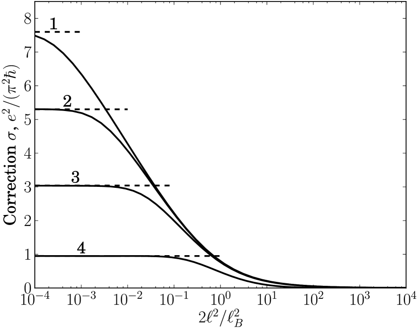
Figure 1: Weak localization correction to conductivity as a function of magnetic field. Curves 1, 2, 3, and 4 are plotted for $\tau/\tau_{\phi}=10^{-4}$, $10^{-3}$, $10^{-2}$, and $10^{-1}$, respectively. Dashed lines show the weak-localization corrections to conductivity at zero magnetic field

Equations (17) and (18) allow us to analyze the behavior of conductivity in low and high magnetic fields. In the low-field limit, the contributions to magnetoconductivity assume the form

$$\sigma_{a}(B)-\sigma_{a}(0)=-\frac{2e^{2}}{\pi^{2}\hbar}F_{2}\left(\frac{4\tau_{\phi}}{\tau}\frac{\ell^{2}}{\ell_{B}^{2}}\right)\>,$$ (20)

$$\sigma_{b}(B)-\sigma_{b}(0)=\frac{e^{2}}{\pi^{2}\hbar}F_{2}\left(\frac{4\tau_{\phi}}{\tau}\frac{\ell^{2}}{\ell_{B}^{2}}\right)\>,$$

where $F_{2}(x)=\ln x+\psi(1/2+1/x)$, $\psi$ is the digamma function. These dependences are in agreement with the result of Ref. McCann, obtained in the diffusion approximation. In the inset of Fig. 2, we compare the magnetoconducitivity $\sigma(B)-\sigma(0)$ calculated after accurate Eqs. (17) and (18) (solid curves) with that calculated in the diffusion approximation Eqs. (20) (dashes curves). One can see that the diffusion approximation describes the magnetoconductivity in low fields, where $\ell_{B}>\ell$. In higher magnetic fields, the diffusion approximation is not valid and one has to use the microscopic theory developed in this paper to describe the magnetoconductivity. Particularly, the ratio 2:1 between $|\sigma_{a}(B)-\sigma_{a}(0)|$ and $|\sigma_{b}(B)-\sigma_{b}(0)|$ obtained in the diffusion approximation does not hold any more. In the high-field limit, i.e., $\ell_{B}\ll\ell$, we may keep only first order in $\ell_{B}/\ell$ terms in Eq. (12), which gives $\sigma\propto 1/\sqrt{B}$.

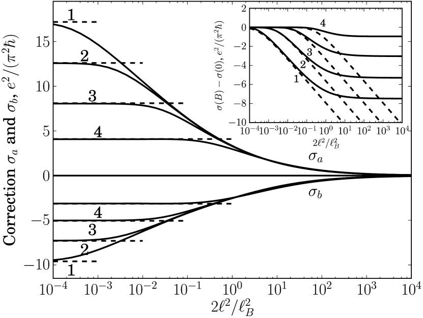
Figure 2: Magnetic field dependences of the contributions $\sigma_{a}$ and $\sigma_{b}$. Curves are plotted for the same ratios $\tau/\tau_{\phi}$ as in Fig. 1. Inset illustrates the dependences $\sigma(B)-\sigma(0)$ on magnetic field calculated after accurate Eqs. (17) and (18) (solid curves) and in the diffusion approximation (dashes curves)

The absolute value of the weak-localization correction to conductivity in zero magnetic field can be obtained from Eqs. (17) and (18) by taking a formal limit $\ell/\ell_{B}\rightarrow 0$. The calculated $\sigma(0)$, $\sigma_{a}(0)$, and $\sigma_{b}(0)$ are shown in Figs. 1 and 2 by dashed lines. The correction $\sigma(0)$ is determined by the phase breaking time, which can be used to experimentally study the dependence of $\tau_{\phi}$ upon temperature or carrier density.

Finally, we note that the presented theory can be applied to describe the weak localization of two-dimensional Dirac fermions in conducting surface of bulk topological insulators. In such systems, there is one two-dimensional channel and the conductivity corrections are given by Eqs. (17) and (18) divided by $4$.

To summarize, we have developed the theory of weak localization for graphene beyond the diffusion regime and calculated the interference corrections to conductivity in the whole range of classically weak magnetic fields. The theory will allow one to better describe experimental data and more precisely determine the phase relaxation time of electrons in graphene.

References

• (1) A.K. Geim and K.S. Novoselov, Nature Mat. 6, 183 (2007).
• (2) N.M.R. Peres, Rev. Mod. Phys. 82, 2673 (2010).
• (3) S. Hikami, A.I. Larkin, and Y. Nagaoka, Prog. Theor. Phys. 63, 707 (1980).
• (4) S.V. Morozov, K.S. Novoselov, M.I. Katsnelson, F. Schedin, L.A. Ponomarenko, D. Jiang, and A.K. Geim, Phys. Rev. Lett. 97, 016801 (2006).
• (5) X. Wu, X. Li, Zh. Song, C. Berger, and Walt A. de Heer, Phys. Rev. Lett. 98, 136801 (2007).
• (6) R.V. Gorbachev, F.V. Tikhonenko, A.S. Mayorov, D.W. Horsell, and A.K. Savchenko, Phys. Rev. Lett. 98, 176805 (2007).
• (7) F.V. Tikhonenko, D.W. Horsell, R.V. Gorbachev, and A.K. Savchenko, Phys. Rev. Lett. 100, 056802 (2008).
• (8) D.-K. Ki, D. Jeong, J.-H. Choi, H.-J. Lee, and K.-S. Park, Phys. Rev. B 78, 125409 (2008).
• (9) X.-Zh. Yan and C.S. Ting, Phys. Rev. Lett. 101, 126801 (2008).
• (10) F.V. Tikhonenko, A.A. Kozikov, A.K. Savchenko and R.V. Gorbachev, Phys. Rev. Lett. 103, 226801 (2009).
• (11) J. Moser, H. Tao, S. Roche, F. Alzina, C.M. Sotomayor Torres, and A. Bachtold, Phys. Rev. B 81, 205445 (2010).
• (12) E. McCann, K. Kechedzhi, V.I. Fal’ko, H. Suzuura, T. Ando, and B.L. Altshuler, Phys. Rev. Lett. 97, 146805 (2006).
• (13) A.F. Morpurgo and F. Guinea, Phys. Rev. Lett. 97, 196804 (2006).
• (14) P.M. Ostrovsky, I.V. Gornyi, and A.D. Mirlin, Phys. Rev. B 74, 235443 (2006).
• (15) K. Kechedzhi, V.I. Fal’ko, E. McCann, and B.L. Altshuler, Phys. Rev. Lett. 98, 176806 (2007).
• (16) J.P. Robinson, H. Schomerus, L. Oroszlany, and V.I. Fal’ko, Phys. Rev. Lett. 101, 196803 (2008).
• (17) F. von Oppen, F. Guinea, and E. Mariani, Phys. Rev. B 80, 075420 (2009).
• (18) K.-I. Imura, Y. Kuramoto, and K. Nomura, Phys. Rev. B 80, 085119 (2009).
• (19) A. Kawabata, J. Phys. Soc. Jpn. 53, 3540 (1984).
• (20) V.M. Gasparian and A.Yu. Zyuzin, Fiz. Tverd. Tela 27, 1662 (1985) [Sov. Phys. Solid State 27, 1580 (1985)].
• (21) M.I. Dyakonov, Solid State Commun. 92, 711 (1994).
• (22) J.E. Moore, Nature 464, 194 (2010).
• (23) Zh. Ren, A.A. Taskin, S. Sasaki, K. Segawa, and Y. Ando, Phys. Rev. B 82, 241306 (2010).
• (24) B. Büttner, C.X. Liu, G. Tkachov, E.G. Novik, C. Brüne, H. Buhmann, E.M. Hankiewicz, P. Recher, B. Trauzettel, S.C. Zhang, and L.W. Molenkamp, Nature Phys. (2011) (in press, doi:10.1038/nphys1914); arXiv:1009:2248.
• (25) H.-T. He, G. Wang, T. Zhang, I.-K. Sou, G.K.L. Wong, J.-N. Wang, H.-Zh. Lu, S.-Q. Shen, and F.-Ch. Zhang, unpublished, arXiv:1008.0141 (2010).
• (26) J. Chen, H.J. Qin, F. Yang, J. Liu, T. Guan, F.M. Qu, G.H. Zhang, J.R. Shi, X.C. Xie, C.L. Yang, K.H. Wu, Y.Q. Li, and L. Lu, Phys. Rev. Lett. 105, 176602 (2010).
• (27) E.B. Olshanetsky, Z.D. Kvon, G.M. Gusev, N.N. Mikhailov, S.A. Dvoretsky, and J.C. Portal, JETP Lett. 91, 347 (2010).
• (28) $V_{\alpha\beta}(-{\bf k},-{\bf k}^{\prime})=V_{\tilde{\beta}\tilde{\alpha}}({\bf k}^{\prime},{\bf k})$ in multi-valley systems (with $\tilde{\alpha}$ and $\tilde{\beta}$ denoting the valleys connected with $\alpha$ and $\beta$, respectively, by time inversion), which leads to a diffusion pole in inter-valley Cooperons. These Cooperons contribute to conductivity giving rise to weak localization in the presence of inter-valley scattering.McCann ; Kuntsevich07
• (29) A.Yu. Kuntsevich, N.N. Klimov, S.A. Tarasenko, N.S. Averkiev, V.M. Pudalov, H. Kojima, and M.E. Gershenson, Phys. Rev. B 75, 195330 (2007).
• (30) A.P. Dmitriev, V.Yu. Kachorovskii, and I.V. Gornyi, Phys. Rev. B 56, 9910 (1997).