A method to identify and characterise binary candidates -
a study of CoRoT   data

Abstract

The analysis of the CoRoT space mission data was performed aiming to test a method that selects, among the several light curves observed, the transiting systems that likely host a low-mass star orbiting the main target. The method identifies stellar companions by fitting a model to the observed transits. Applying this model, that uses equations like Kepler’s third law and an empirical mass-radius relation, it is possible to estimate the mass and radius of the primary and secondary objects as well as the semimajor axis and inclination angle of the orbit. We focus on how the method can be used in the characterisation of transiting systems having a low-mass stellar companion with no need to be monitored with radial-velocity measurements or ground-based photometric observations. The model, which provides a good estimate of the system parameters, is also useful as a complementary approach to select possible planetary candidates. A list of confirmed binaries together with our estimate of their parameters are presented. The characterisation of the first twelve detected CoRoT exoplanetary systems was also performed and agrees very well with the results of their respective announcement papers. The comparison with confirmed systems validates our method, specially when the radius of the secondary companion is smaller than 1.5 ${\rm R}_{\rm Jup}$, in the case of planets, or larger than 2 ${\rm R}_{\rm Jup}$, in the case of low-mass stars. Intermediate situations are not conclusive.

1 Introduction

The analysis of transiting systems based on light curve modelling combined with ground-based follow-up by means of radial-velocity measurements have shown their exceptional importance in the characterisation of extrasolar systems. Together, they provide the determination of several physical and orbital parameters that cannot normally be obtained for non-transiting systems, such as the mass and radius of the secondary companion, and thus its density. The possibility of a detailed study of extrasolar transiting light curves in a large number of targets has been considerably improved by recent photometric space missions, such as CoRoT (Baglin et al. 2006) and Kepler (Borucki et al. 2010).

At the time of this writing the CoRoT space telescope has collected, since its launch, the light curves of more than a hundred thousand stars through 13 observational runs. This huge number of stars is a strong motivation to develop tools to efficiently treat the released data, specially considering that first of all the data need to be cleaned from long-term variations, short-term oscillations, outliers, discontinuities, and others. Regarding the characterisation of extrasolar systems, an extra challenge is to distinguish transits caused by planetary companions from those related to the presence of a low-mass star in a binary system, particularly given the time-consuming ground-based observations that are normally used as a complementary approach.

Carpano et al. (2009) published their results concerning the analysis of CoRoT light curves observed during the initial run of the mission, named IRa01, in which they presented a list of 50 planetary candidates together with a list of 145 eclipsing binary candidates. Moutou et al. (2009) complemented the work of Carpano et al. (2009) with additional follow-up observations, also in the context of the initial run. In other two papers, published by Deeg et al. (2009) and Cabrera et al. (2009), the authors presented a list of targets for which ground-based follow-up was conducted, helping as a complementary approach in the classification of the candidates. The lists released by these papers are the result of a huge effort of several working groups, and shows how difficult it is to characterise systems, planetary candidates or not, among thousands of targets.

In the work of Silva & Cruz (2006), the authors proposed a method based on the fit of light curves with transits that can be used in the characterisation of transiting systems. This method provides the determination of some parameters of the system, such as the orbital inclination angle, the semimajor axis, and the mass and radius of the primary and secondary objects. In the present work we have used an updated version of the same method, applied to a list of transiting light curves from publicly available runs of the CoRoT mission. The purpose of our analysis is to show that the method is useful to identify transits most likely caused by a binary configuration, without making use of any time-consuming effort to conduct ground-based follow-up, like radial velocity measurements or photometric observations.

Silva & Cruz (2006) also tested their model applied to the transiting exoplanetary systems known at that time, and their results are in good agreement with the published parameters. Therefore, here we analysed the first confirmed CoRoT planetary systems as well, from CoRoT-1 through 12, comparing our estimates to those in their respective announcement papers.

Section 2 presents the data reduction, showing the corrections needed to apply to the light curves (in the format delivered to the scientific community) before modelling the transit shape. Next, Sect. 3 describes the method and its usefulness in the classification of binary system candidates. In Sect. 4, the results are presented and discussed, which includes our parameter estimate for a list of binary systems first identified by other works as well as the characterisation of confirmed CoRoT exoplanetary systems. Finally, Sect. 5 presents the final remarks and conclusions.

2 Sample data and reduction

The light curves analysed using our method are part of the three-colour band data from publicly available runs observed by the CoRoT mission (a few cases of monochromatic light curves were also included). Before doing any kind of fit to model the observed transits, the light curves have to be cleaned from any systematic noise that may still remain in the data delivered to the scientific community, which format is called the N2 level (Baudin et al. 2006). The systematic noise normally seen is related to: $i)$ discontinuities produced by hot pixels; $ii)$ outliers, whose sources are diverse; and $iii)$ short-term oscillations related to the CoRoT orbital frequency (103 min) and its harmonics. For details on the CoRoT satellite and its orbit see e.g. Boisnard & Auvergne (2006) and Auvergne et al. (2009). In addition to the systematic noise, short-term oscillations, intrinsic to some type of stars, were also observed in some light curves and removed.

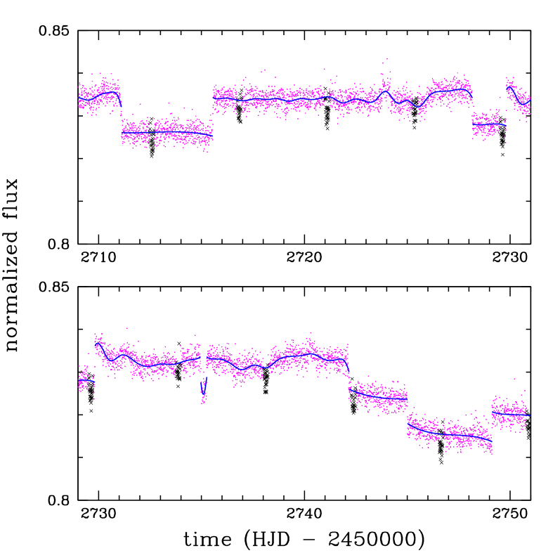
Figure 1: Example of polynomial function fit performed to correct the light curves from eventual discontinuities. Only points within twice $\sigma$ and located outside transits (dots) are taken into account when searching for the best fit (solid lines). Transit positions are represented by crosses. This figure represents CoRoT-1, which folded light curve is shown in Fig. 6 after the discontinuity corrections were made.

We developed a code to correct the light curves from discontinuities and outliers. The code computes the first derivate of the data points in order to locate the discontinuities, then it fits polynomial functions to points between them, and finally the light curve is normalised according to such functions. When searching for the best fit, the code does not consider: $i)$ data points located outside twice $\sigma$, which value is estimated in a specific portion of the light curve; and $ii)$ data points located where transits happen. We note that a visual inspection is always conducted to avoid any abrupt behaviour of the fitted function, specially close to transit times. Figure 1 shows an example of this polynomial function fit.

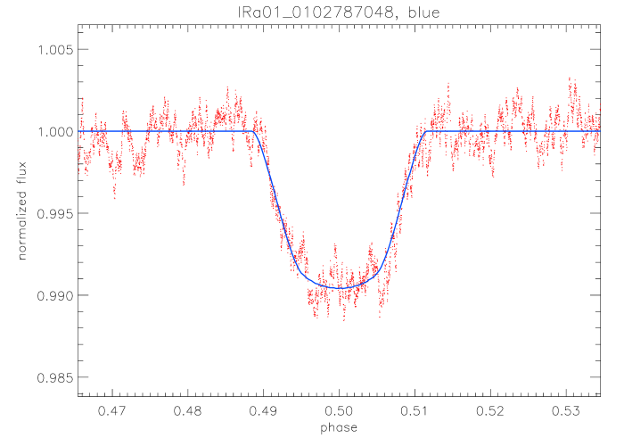
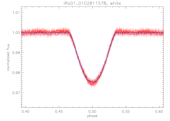
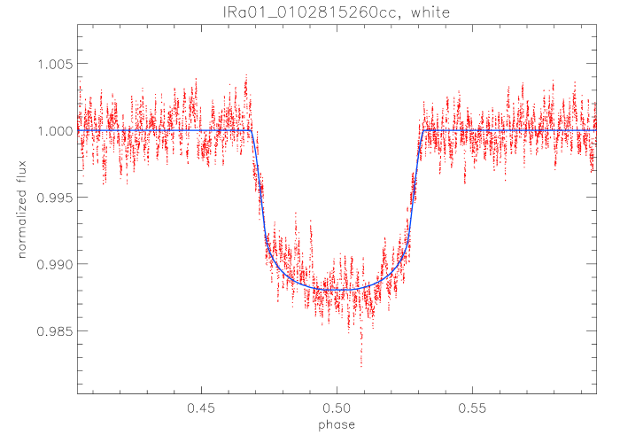
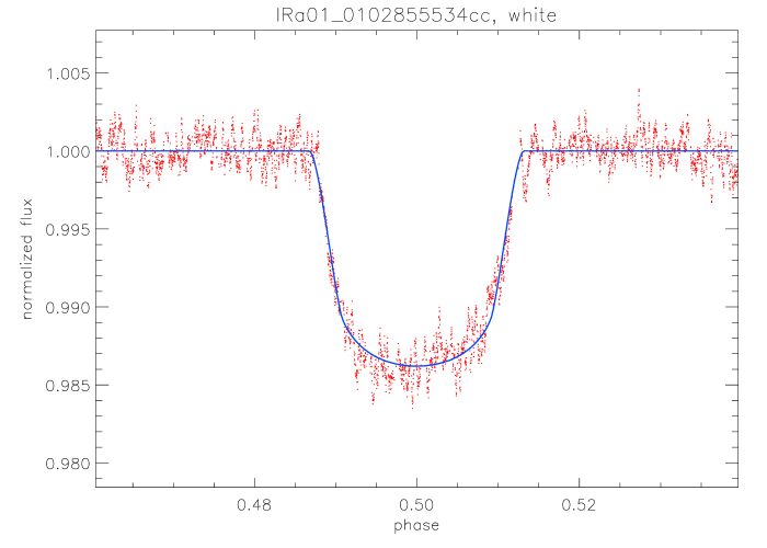
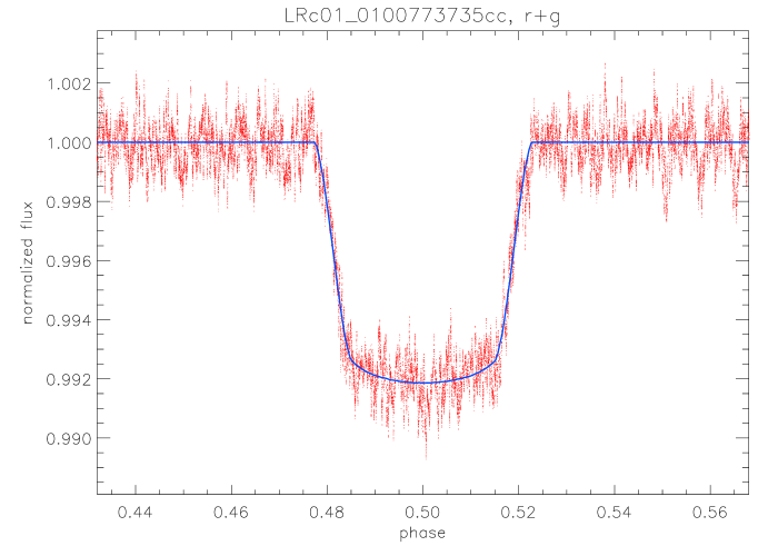
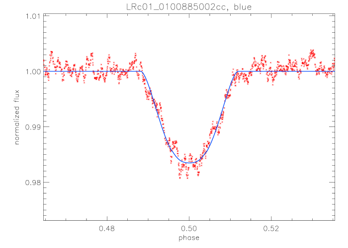
Figure 5: Examples of binary systems analysed in the present work. Here and in the following figure the light curves were smoothed to reduce noise and clarify visualisation. The index $c$, when added to the CoRoT ID, indicates that the light curve was corrected from short-period oscillations.

Short-term oscillations may also affect the search for the model that best fits the observed transit. Figure 2 shows an example of a transiting light curve when this kind of oscillation is present. The same object is shown in Fig. 5 after being corrected from the most prominent harmonics. Oscillations due to the intrinsic variability of some stars were also properly removed when needed.

3 Light curve fit

The method developed by Silva & Cruz (2006) was used here to search for the best model parameters that fit the observed light curve transits. The model considers an opaque disc that simulates the secondary object passing across the stellar disc. We assumed a quadratic function to describe the limb-darkening of the disc of the primary object, which is based on the star HD 209458 ($u_{1}=0.2925$ and $u_{2}=0.3475$, from Brown et al. 2001). An exception is the system 0100773735 (LRc01, Fig. 5), for which $u_{1}$ and $u_{2}$ were assumed to be half those of the star HD 209458. In the case in which the secondary companion is a low-mass star, it will not be an opaque disc. However, this will not considerably change the results, since its flux contribution is small compared to the main star (a 0.3 ${\rm M}_{\odot}$ star orbiting a solar-type star contributes less than 2% to the total flux). Cases in which the secondary is as bright as the primary were not selected in our analysis given the large transit depth that would be observed in the light curve.

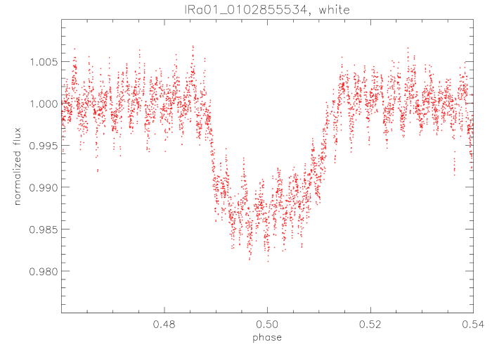
Figure 2: Phase-folded light curve with short-term oscillations (in this case due to the CoRoT orbit) that we have to correct before modelling the transit shape. The same system is shown in Fig. 5 after these oscillations have been removed.

The orbital period ($P$) of the companion is a known parameter, obtained directly from the light curve, whereas the following three variables are the result of the best fit: the radii ratio between secondary and primary objects ($R_{\rm p}=R_{2}/R_{1}$), the semimajor axis of the secondary orbit in units of the primary radius ($a_{\rm p}=a/R_{1}$), and the orbital inclination angle ($i$). The search for the best fit is conducted with the AMOEBA routine (Press et al. 1992), which performs a multidimensional chi-square ($\chi^{2}$) minimisation of the function $f$($R_{\rm p}$, $a_{\rm p}$, $i$) describing the transit profile.

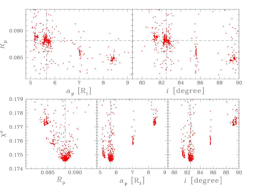
Figure 3: Example of $\chi^{2}$ minimisation for the system 0100773735 (LRc01, Fig. 5) in the search for values of $R_{\rm p}$, $a_{\rm p}$, and $i$ of the model that best fit the observed transit.

The first set of parameters normally used as input are: $R_{\rm p}$ = 0.1, $i=85^{\circ}$, and $a_{\rm p}=a/R_{1}$ calculated according to the Kepler’s third law (Equation 3) for $M_{1}+M_{2}\sim 1$ ${\rm M}_{\odot}$ and $R_{1}\sim 1$ ${\rm R}_{\odot}$. In order to avoid premature convergences on local minimums and explore the entire parameter space, the best solution is found after running the routine several times, replacing the input parameters by new values within a chosen range (e.g. $\Delta R_{\rm p}=\pm 0.05$, $\Delta a_{\rm p}=\pm 3.0~{}R_{1}$, and $\Delta i=\pm 5^{\circ}$). Throughout the execution of the process, a visual inspection of the fit is carried out after each possible solution is achieved. Figure 3 shows an example of $\chi^{2}$ minimisation for the system 0100773735 (LRc01).

3.1 Estimate of mass and radius

The method used to estimate the mass and radius of the primary and secondary companion was updated using new mass-radius relations based on more recent discoveries, specially the one fitted to known exoplanets (systems presently listed in the Extrasolar Planets Encyclopaedia were used). These relations are:

$$R=A{M}^{B}$$ (1)

$$R=C{M}+D$$ (2)

where $A=0.013938$, $B=3.867270$, $C=0.410162$, and $D=0.065934$. The function given by Equation 1 was fitted to stars whereas Equation 2 represents a function fitted to known exoplanets and the planets of the solar system. Both functions are plotted in Fig. 4. Exoplanets having radius $>1$ ${\rm R}_{\rm Jup}$ or mass $>2$ ${\rm M}_{\rm Jup}$ and low-mass objects having radius $<2$ ${\rm R}_{\rm Jup}$ were not used in the search for the best fit. These objects belong to an ambiguous region of the mass-radius diagram, in which a change in mass does not necessarily imply in a change in radius.

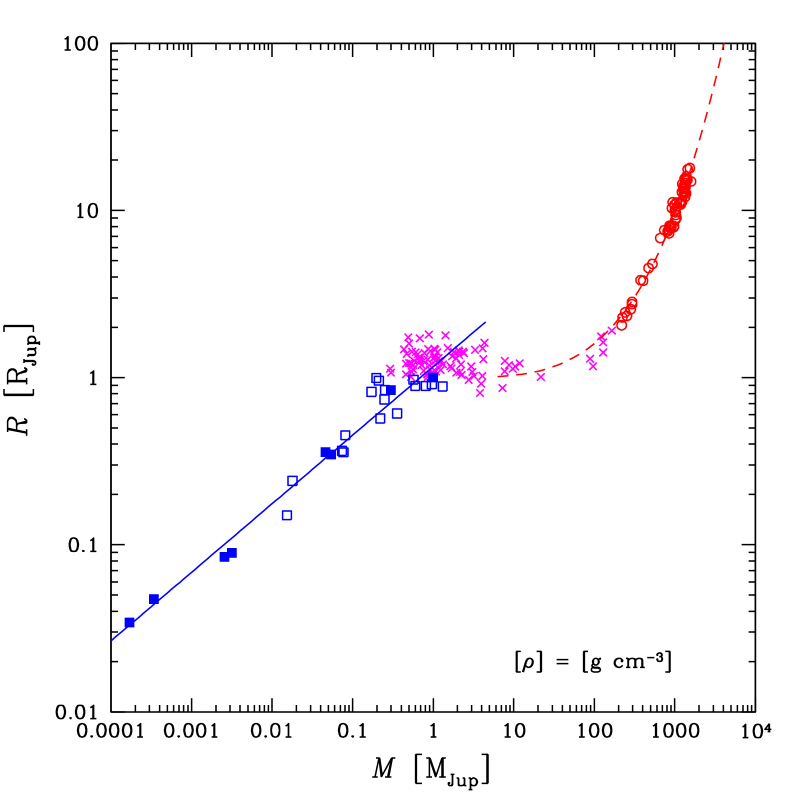
Figure 4: Empirical mass-radius relations used by our method. The long-dashed line is a function, given by Equation 1, fitted to stars (open circles) whereas the solid line represents a function, given by Equation 2, fitted to known exoplanets (open squares) and the planets of the Solar System (filled squares). Crosses represent exoplanets and low-mass objects that were not used in the fit (see text). The values of mass and radius were taken from the Extrasolar Planets Encyclopaedia³.

After applying our method to the observed transits, we are able to estimate the mass and radius of both the primary ($M_{1}$, $R_{1}$) and secondary ($M_{2}$, $R_{2}$) objects and the orbital semimajor axis $a$ (given in astronomical units) using the following relations:

$$a^{3}=\frac{GP^{2}}{4\pi^{2}}(M_{1}+M_{2})$$ (3)

$$R_{\rm p}=\frac{R_{2}}{R_{1}}$$ (4)

$$a_{\rm p}=\frac{a}{R_{1}}$$ (5)

$$R_{1}=A{M_{1}}^{B}, R_{2}=A{M_{2}}^{B}$$ (6)

$$R_{1}=A{M_{1}}^{B}, R_{2}=C{M_{2}}+D$$ (7)

where Equation 3 is the Kepler’s third law, Equations 4 and 5 are obtained by the transit best fit, and Equations 6 and 7 are the empirical mass-radius relations used depending on whether the secondary companion is a star or a planet. Therefore, two sets of five relations are numerically solved and two sets of the parameters $M_{1}$, $R_{1}$, $M_{2}$, $R_{2}$, and $a$ are computed. If $R_{2}\gtrsim 2$ ${\rm R}_{\rm Jup}$ then we consider the system to be a binary candidate and the parameters yielded by Equations 3, 4, 5, and 6 are used. On the other hand, if $R_{2}<2$ ${\rm R}_{\rm Jup}$, then the parameters yielded by Equations 3, 4, 5, and 7 are used.

The numerical calculation of $M_{1}$, $R_{1}$, $M_{2}$, $R_{2}$, and $a$ proceeds as follows: first, one of the parameters is fixed (e.g. $M_{1}$ = 1 ${\rm M}_{\odot}$) and the others are calculated; then, the ratio $a/R_{1}$ is compared to the value of $a_{\rm p}$ provided by the transit best fit; the fixed parameter is iteratively incremented (or decremented) until the difference between $a/R_{1}$ and $a_{\rm p}$ is as smaller as one wishes. When this condition is satisfied, the five parameters are finally estimated.

Concerning the mass of the secondary objects ($M_{2}$), there are three possibilities: $i)$ if the companion has $R_{2}>2$ ${\rm R}_{\rm Jup}$, then it will probably be a low-mass star and its mass can be easily estimated by the mass-radius relation fitted to that region of the diagram; $ii)$ if $R_{2}<1$ ${\rm R}_{\rm Jup}$, then we can estimate a value for $M_{2}$ using the other mass-radius relation; however, since the mass-radius relation for planets depends on their chemical composition, it is not possible to estimate an accurate mass value for the secondary in this radius regime if its composition is unknown; $iii)$ finally, if $1\leq\ R_{2}\leq\ 2$ ${\rm R}_{\rm Jup}$, then the mass can not be univocally determined since, for one given radius, objects in this radius regime may have masses ranging from about $1~{}$${\rm M}_{\rm Jup}$ to about $100~{}$${\rm M}_{\rm Jup}$ (brown dwarfs). Based on these arguments, we only include in our discussion a mass estimate for secondary companions with $R_{2}\gtrsim 2$ ${\rm R}_{\rm Jup}$. Nevertheless, we note that our method provides a good estimate for the radius of not only primary and secondary stars, but also of planetary companions (even for $R_{2}<2$ ${\rm R}_{\rm Jup}$). Indeed, this is the case of the confirmed CoRoT systems, which results are presented and discussed in Sect. 4.

3.2 Uncertainties in the system parameters

The results presented here are for the parameters $a$, $i$, $M_{1}$, $R_{1}$, $M_{2}$, and $R_{2}$, where $a$ is given in astronomical units, $M_{1}$ and $M_{2}$ in solar masses, $R_{1}$ in solar radii, and $R_{2}$ in Jupiter radii. To estimate the uncertainty in these parameters, the procedure is as follows:

• first, the standard deviation ($\sigma$) is computed in a region outside a transit for the model that best fits the light curve; in a region inside a transit, a possible presence of spots on the surface of the primary star would cause variations in the light curve (Silva 2003) and $\sigma$ would be miscalculated;

• by changing, at a given step, the three basic parameters yielded from the best fit to the transit ($R_{\rm p}$, $a_{\rm p}$, and $i$), we obtain a new light curve;

• next, these parameters are changed until the new light curve starts deviating significantly from the best one; that is when the difference between the light curves is more than 1 $\sigma$ for at least 10% of the transit;

• finally, these new basic parameters are used to re-estimate $M_{1}$, $M_{2}$, $R_{1}$, and $R_{2}$ following the procedure described in Sect. 3.1; the difference between both new and best estimates provides the uncertainties in the parameters.

Our mass-radius relations (Equations 1 and 2) do not depend directly on the orbital inclination angle. However, since a change in this parameter leads to a change in both depth and duration of the transit, its uncertainty can be included in the uncertainty determination of the other two basic parameters. To do so, first the uncertainty in the inclination angle is estimated as described above (in steps 2 and 3 only $i$ is changed). Then, the uncertainties in the other two parameters (each one in turn) are estimated considering the inclination angle changed by its uncertainty. At the end, the uncertainties in $M_{1}$, $R_{1}$, $M_{2}$, and $R_{2}$ take into account those in $R_{\rm p}$, $a_{\rm p}$, and $i$. The uncertainty in $a$ includes those in both $a_{\rm p}$ and $R_{1}$ given the conversion of the semimajor axis from units of stellar radius to astronomical units.

To reduce noise and clarify visualisation, a smoothing function was applied to the light curves before searching for the model that best fits the transit. In addition, for some systems only the best quality channels were used in the analysis. These procedures result in a more accurate estimate of the system parameters and, consequently, in smaller uncertainties.

4 Results and discussion

4.1 Characterisation of binary system candidates

Table 1 and Fig. 5 show a few examples of our method applied to light curves of systems classified as eclipsing binaries or targets having faint background eclipsing binary stars.

Table 1: Physical and orbital parameters for CoRoT systems analysed in this work. The uncertainties in $a$, $i$, $M_{1}$, $R_{1}$, $M_{2}$, and $R_{2}$ were estimated as described in Sect. 3.2. These targets represent confirmed or probable binary systems and they are all commented in Sect. 4.1.

CoRoT ID	Run	$P$ [days]	$a$ [AU]	$i$ [deg]	$M_{1}$ [${\rm M}_{\odot}$]	$R_{1}$ [${\rm R}_{\odot}$]	$M_{2}$ [${\rm M}_{\odot}$]	$R_{2}$ [${\rm R}_{\rm Jup}$]	Ref.
0102787048	IRa01	7.896	0.094 $\pm$ 0.008	85.1 $\pm$ 0.2	1.63 $\pm$ 0.08	2.1 $\pm$ 0.2	0.16 $\pm$ 0.07	2.00 $\pm$ 0.31	[2, 3, 4]
0102811578	IRa01	1.66882	0.0339 $\pm$ 0.0008	77.1 $\pm$ 0.2	1.57 $\pm$ 0.02	1.95 $\pm$ 0.04	0.32 $\pm$ 0.02	3.09 $\pm$ 0.17	[2]
0102815260	IRa01	3.587	0.057 $\pm$ 0.006	$>$ 87.0	1.71 $\pm$ 0.09	2.2 $\pm$ 0.2	0.19 $\pm$ 0.08	2.14 $\pm$ 0.31	[2, 4]
0102855534	IRa01	21.72	0.218 $\pm$ 0.014	86.9 $\pm$ 0.2	2.48 $\pm$ 0.07	4.2 $\pm$ 0.2	0.50 $\pm$ 0.05	4.49 $\pm$ 0.42	[2, 4]
0100773735	LRc01	4.974	0.074 $\pm$ 0.004	82.5 $\pm$ 0.2	1.98 $\pm$ 0.06	2.8 $\pm$ 0.1	0.23 $\pm$ 0.04	2.42 $\pm$ 0.24	[1]
0100885002	LRc01	11.8054	0.136 $\pm$ 0.007	85.1 $\pm$ 0.1	2.02 $\pm$ 0.02	2.9 $\pm$ 0.1	0.42 $\pm$ 0.04	3.80 $\pm$ 0.31	[1]
0101482707	LRc01	39.89	0.270 $\pm$ 0.004	88.5 $\pm$ 0.1	1.45 $\pm$ 0.01	1.73 $\pm$ 0.02	0.19 $\pm$ 0.01	2.18 $\pm$ 0.09	[1]
0101095286	LRc01	5.053	0.088 $\pm$ 0.005	70.6 $\pm$ 0.4	3.2 $\pm$ 0.1	6.7 $\pm$ 0.3	0.43 $\pm$ 0.12	3.91 $\pm$ 0.92	[1, 3]
0101434308	LRc01	79.95	0.41 $\pm$ 0.02	$>$ 89.7	1.30 $\pm$ 0.05	1.46 $\pm$ 0.08	0.18 $\pm$ 0.06	2.10 $\pm$ 0.17	[1]
0211660858	SRc01	8.825	0.114 $\pm$ 0.008	86.3 $\pm$ 0.3	2.12 $\pm$ 0.07	3.2 $\pm$ 0.2	0.46 $\pm$ 0.05	4.10 $\pm$ 0.38
0211654447	SRc01	4.751	0.090 $\pm$ 0.005	70.9 $\pm$ 0.4	3.3 $\pm$ 0.1	7.4 $\pm$ 0.3	1.04 $\pm$ 0.10	9.90 $\pm$ 1.23
0102755837	LRa01	27.955	0.28 $\pm$ 0.02	83.8 $\pm$ 0.2	3.4 $\pm$ 0.1	7.6 $\pm$ 0.4	0.48 $\pm$ 0.07	4.28 $\pm$ 0.61

[1] Cabrera et al. (2009); [2] Carpano et al. (2009); [3] Deeg et al. (2009); [4] Moutou et al. (2009).

According to Silva & Cruz (2006), the present method should consider as non-planetary candidates only the systems for which the radius of the secondary companion is larger than 1.5 Jupiter radii. After that publication, some exoplanets with radius between 1.5 and 2 ${\rm R}_{\rm Jup}$ were discovered. Thus, in this work, we chose a more conservative value of $R_{2}$ = 2 ${\rm R}_{\rm Jup}$ for the lower limit of binary candidates.

The systems that our method classify as binary candidates actually represent classes of systems with different configurations of the components. There are several sources of false alarms that can mimic the transit of a planet in front of the main target. The most common are eclipsing binary systems with grazing transits, targets having a background eclipsing binary system, or even triple systems. The present method does not identify the exact configuration of the system, but provides the information that the observed transits are likely not caused by a planet. Listed below are our comments for each case. The window ID of the run (e.g. E1-0288) is also shown as a complementary identifier.

IRa01 - 0102787048 (E1-0288)

This system was first classified by Carpano et al. (2009) as a planetary transit candidate. However, after follow-up observations, Moutou et al. (2009) confirmed that the transit is originated by a background eclipsing binary and then diluted by the main target. They estimated a mass-ratio of 0.15 between secondary and primary components of the binary system. Using the results of our method we have a value of 0.10 $\pm$ 0.04 for the same ratio, which is consistent with a diluted transit of a more massive object. The fact that no transit is observed in the red channel also helped to label a non-planetary nature for this target.

IRa01 - 0102811578 (E2-0416)

System classified by Carpano et al. (2009) as an eclipsing binary. No information concerning follow-up observations has been published. Our estimate of mass and radius for the secondary companion confirms its binary nature.

IRa01 - 0102815260 (E2-2430)

Also in the list of planetary transit candidates of Carpano et al. (2009), but afterwards classified by Moutou et al. (2009) as a binary system according to radial-velocity observations. Our estimate for the mass-ratio is 0.11 $\pm$ 0.04, slightly smaller than the value of 0.17 published by Moutou et al. (2009), but still consistent with a stellar companion.

IRa01 - 0102855534 (E2-1736)

Follow-up observations conducted by Moutou et al. (2009) indicate that an eclipsing binary is the main target, changing the planetary nature of the secondary first suggested by Carpano et al. (2009). The radial-velocity measurements indicate a mass-ratio of 0.2, which agrees with our estimate of 0.19 $\pm$ 0.01. Indeed, the mass and radius that we show in Table 1 clearly indicate the stellar nature of the secondary.

LRc01 - 0100773735 (E2-1245)

Based on radial-velocity observations, Cabrera et al. (2009) suggest that this is a spectroscopic binary or multiple system. Our mass and radius estimate confirms their conclusion of a non-planetary object causing the observed transits.

LRc01 - 0100885002 (E2-4653)

This target is listed in Cabrera et al. (2009) as an eclipsing binary, which is in agreement with the mass and radius estimated using our method. Transits are observed only in the blue channel, contributing to the classification of this system as non-planetary.

LRc01 - 0101482707 (E1-2837)

Also classified by Cabrera et al. (2009) as a binary system after radial-velocity observations and confirmed by our method.

LRc01 - 0101095286 (E1-2376)

The follow-up of this target with photometric observations unveiled its binary nature (Cabrera et al. 2009), which can be clearly confirmed by our results of mass and radius for the secondary object.

LRc01 - 0101434308 (E1-3425)

Cabrera et al. (2009), without doing any follow-up observations, concluded that this is a binary system given the fact that the transit is predominantly seen in the blue channel.

In Table 1 are also listed our results for the targets 0211660858 (SRc01, E2-0369), 0211654447 (SRc01, E1-1165), and 0102755837 (LRa01, E2-2249). The CoRoT team has not yet published the results of their analysis for these runs. Nevertheless, they are shown here because the secondary mass and radius estimated by our method clearly classify these targets as non-planetary systems.

As one can see in Table 1, for some targets the estimated radius of the secondary companion is close to the limit of 2 ${\rm R}_{\rm Jup}$ used to distinguish binaries from possible planetary systems. They were classified as probable binary systems considering that, at present, all detected exoplanets for which the radius was derived are as large as 1.8 ${\rm R}_{\rm Jup}$ or smaller.

Among the nine targets listed in Table 1 that were analysed and published by the CoRoT team, six were classified as binary systems only after ground-based follow-up, either by radial-velocity measurements, or by photometric observations, or both. This is an indication that the method normally used by different CoRoT working groups is perhaps not good enough to provide a pre-classification of the targets. Our method would exclude the binary targets by itself, and no time-consuming follow-up observations would be required for most cases.

4.2 Characterisation of exoplanetary systems

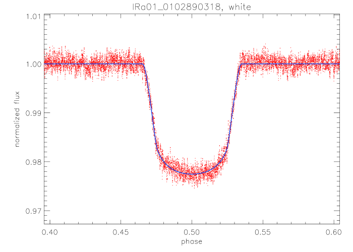
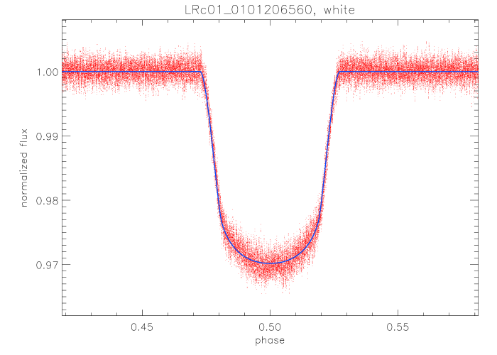
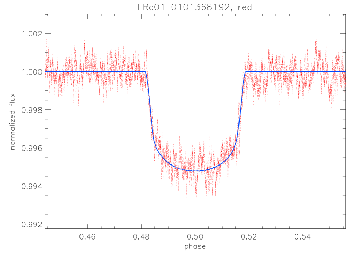
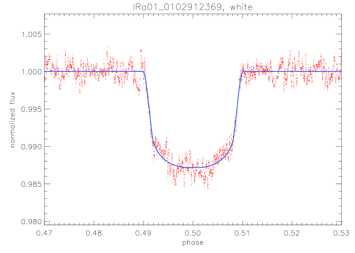
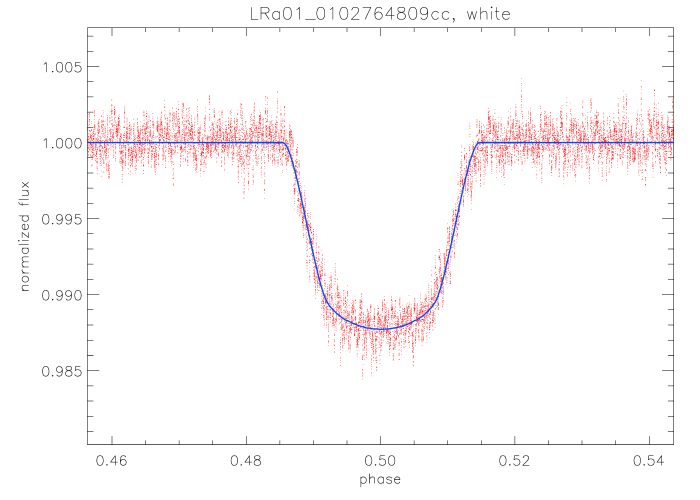
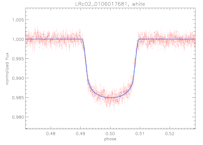
Figure 6: The first six CoRoT exoplanetary systems: CoRoT-1 through CoRoT-6, respectively, from left to right and from up to bottom.

Table 2 presents our parameter estimates for confirmed CoRoT exoplanetary systems, from CoRoT-1 through 12, together with the results presented in the announcement papers. Here the method uses the information provided by the mass-radius relation fitted to known transiting exoplanets and to the planets of the solar system (Equation 2, Fig. 4). Figure 6 shows the light curves of the first six CoRoT systems plotted with our best fit.

Table 2: Parameters of the first twelve confirmed CoRoT planetary systems compared to the results of this work. The period values are from the respective announcement papers. The uncertainties in $a$, $i$, $M_{1}$, $R_{1}$, and $R_{2}$ were estimated as described in Sect. 3.2.

CoRoT ID	Run	$P$ [days]	$a$ [AU]	$i$ [deg]	$M_{1}$ [${\rm M}_{\odot}$]	$R_{1}$ [${\rm R}_{\odot}$]	$R_{2}$ [${\rm R}_{\rm Jup}$]	Ref.
0102890318 (CoRoT-1)	IRa01	1.5089557 (64)	0.027 $\pm$ 0.002 0.0254 $\pm$ 0.0004	85.2 $\pm$ 0.5 85.1 $\pm$ 0.5	1.11 $\pm$ 0.04 0.95 $\pm$ 0.15	1.18 $\pm$ 0.06 1.11 $\pm$ 0.05	1.59 $\pm$ 0.13 1.49 $\pm$ 0.08	[0] [1]
0101206560 (CoRoT-2)	LRc01	1.7429964 (17)	0.028 $\pm$ 0.002 0.0281 $\pm$ 0.0009	87.5 $\pm$ 0.4 87.8 $\pm$ 0.1	0.90 $\pm$ 0.03 0.97 $\pm$ 0.06	0.90 $\pm$ 0.04 0.902 $\pm$ 0.018	1.38 $\pm$ 0.10 1.465 $\pm$ 0.029	[0] [2]
0101368192 (CoRoT-3)	LRc01	4.256800 (5)	0.056 $\pm$ 0.005 0.057 $\pm$ 0.003	86.3 $\pm$ 0.4 85.9 $\pm$ 0.8	1.33 $\pm$ 0.07 1.37 $\pm$ 0.09	1.52 $\pm$ 0.11 1.56 $\pm$ 0.09	0.98 $\pm$ 0.13 1.01 $\pm$ 0.07	[0] [3]
0102912369 (CoRoT-4)	IRa01	9.20205 (37)	0.087 $\pm$ 0.006 0.090 $\pm$ 0.001	$>$ 89.3 $>$ 89.915	1.03 $\pm$ 0.04 1.16 $\pm$ 0.03	1.07 $\pm$ 0.06 1.17 $\pm$ 0.03	1.07 $\pm$ 0.10 1.19 $\pm$ 0.06	[0] [4]
0102764809 (CoRoT-5)	LRa01	4.0378962 (19)	0.053 $\pm$ 0.003 0.04947 $\pm$ 0.00029	85.0 $\pm$ 0.2 86 $\pm$ 1	1.19 $\pm$ 0.04 1.00 $\pm$ 0.02	1.29 $\pm$ 0.06 1.19 $\pm$ 0.04	1.37 $\pm$ 0.14 1.388 $\pm$ 0.047	[0] [5]
0106017681 (CoRoT-6)	LRc02	8.886593 (4)	0.083 $\pm$ 0.006 0.0855 $\pm$ 0.0015	89.4 $\pm$ 0.4 89.1 $\pm$ 0.3	0.96 $\pm$ 0.05 1.05 $\pm$ 0.05	0.98 $\pm$ 0.06 1.025 $\pm$ 0.026	1.06 $\pm$ 0.10 1.166 $\pm$ 0.035	[0] [6]
0102708694 (CoRoT-7)	LRa01	0.853585 (24)	0.018 $\pm$ 0.005 0.01720 $\pm$ 0.00029	78.2 $\pm$ 1.5 80.1 $\pm$ 0.3	0.98 $\pm$ 0.17 0.93 $\pm$ 0.03	1.01 $\pm$ 0.23 0.87 $\pm$ 0.04	0.15 $\pm$ 0.07 0.150 $\pm$ 0.008	[0] [7]
0101086161 (CoRoT-8)	LRc01	6.21229 (3)	0.067 $\pm$ 0.004 0.063 $\pm$ 0.001	86.7 $\pm$ 0.1 88.4 $\pm$ 0.1	1.06 $\pm$ 0.03 0.88 $\pm$ 0.04	1.11 $\pm$ 0.05 0.77 $\pm$ 0.02	0.88 $\pm$ 0.09 0.57 $\pm$ 0.02	[0] [8]
0105891283 (CoRoT-9)	LRc02	95.2738 (14)	0.39 $\pm$ 0.02 0.407 $\pm$ 0.005	$>$ 89.87 $>$ 89.95	0.85 $\pm$ 0.03 0.99 $\pm$ 0.04	0.84 $\pm$ 0.04 0.94 $\pm$ 0.04	0.93 $\pm$ 0.08 1.05 $\pm$ 0.04	[0] [9]
0100725706 (CoRoT-10)	LRc01	13.2406 (2)	0.108 $\pm$ 0.005 0.1055 $\pm$ 0.0021	88.0 $\pm$ 0.1 88.6 $\pm$ 0.2	0.94 $\pm$ 0.03 0.89 $\pm$ 0.05	0.95 $\pm$ 0.04 0.79 $\pm$ 0.05	1.15 $\pm$ 0.10 0.97 $\pm$ 0.07	[0] [10]
0105833549 (CoRoT-11)	LRc02	2.994330 (11)	0.044 $\pm$ 0.002 0.044 $\pm$ 0.005	83.2 $\pm$ 0.2 83.17 $\pm$ 0.15	1.24 $\pm$ 0.04 1.27 $\pm$ 0.05	1.37 $\pm$ 0.06 1.37 $\pm$ 0.03	1.32 $\pm$ 0.13 1.43 $\pm$ 0.03	[0] [11]
0102671819 (CoRoT-12)	LRa01	2.828042 (13)	0.040 $\pm$ 0.003 0.0402 $\pm$ 0.0009	85.7 $\pm$ 0.2 85.5 $\pm$ 0.8	1.02 $\pm$ 0.05 1.08 $\pm$ 0.08	1.06 $\pm$ 0.07 1.12 $\pm$ 0.10	1.33 $\pm$ 0.15 1.44 $\pm$ 0.13	[0] [12]

[0] this work; [1] Barge et al. (2008); [2] Alonso et al. (2008); [3] Deleuil et al. (2008); [4] Aigrain et al. (2008); [5] Rauer et al. (2009);

[6] Fridlund et al. (2010); [7] Leger et al. (2009); [8] Bordé et al. (2010); [9] Deeg et al. (2010); [10] Bonomo et al. (2010);

[11] Gandolfi et al. (2010); [12] Gillon et al. (2010)

The results of a detailed comparison between our estimates and those of the announcement papers are shown in Table 3. This table lists the coefficients of weighted linear regressions obtained for $a$, $i$, $M_{1}$, $R_{2}$, and $R_{2}$, where the weights $1/\sigma^{2}$ were used for $\sigma$ representing the errors that we estimated for these parameters. At first, we computed the coefficients using the first twelve CoRoT systems and no systematic difference was found within 2$\sigma$. Within 1$\sigma$, however, the agreement is not so good, specially for $M_{1}$ and $R_{1}$. This is most due to discrepancies in the comparison of CoRoT-8, as one can observe in Table 2. The data points in the light curve of this system has a dispersion of 0.017, which is much larger than those of the other CoRoT systems: $\sim$0.007 or smaller. Indeed, if the parameters of CoRoT-8 are not included in the regressions, the agreement between our results and those of the announcement papers is much better, standing within 1$\sigma$ mostly. An extra caution when dealing with noisy light curves is, therefore, recommended. Light curves with small-depth or long-period transits (such as CoRoT-7 and 9, respectively) also produce larger uncertainties in the parameters and should be carefully analysed.

Table 3: Coefficients of the linear regression obtained in the comparison of the parameters listed in Table 2, with CoRoT-8 included or not (see Sect. 4.2). The angular and linear coefficients ($\alpha$, $\beta$), the dispersion around the fit ($rms$), and the correlation coefficient ($cc$) are shown for both scenarios.

	$\alpha$	$\beta$	$rms$	$cc$
For the first twelve CoRoT systems:
$a$	0.98 $\pm$ 0.02	0.0016 $\pm$ 0.0010	0.0017	1.00
$i$	0.91 $\pm$ 0.12	7 $\pm$ 10	0.68	0.97
$M_{1}$	0.55 $\pm$ 0.27	0.47 $\pm$ 0.28	0.11	0.68
$R_{1}$	0.66 $\pm$ 0.19	0.38 $\pm$ 0.19	0.12	0.84
$R_{2}$	0.88 $\pm$ 0.09	0.11 $\pm$ 0.10	0.13	0.94
CoRoT-8 not included:
$a$	0.97 $\pm$ 0.02	0.0017 $\pm$ 0.0009	0.0015	1.00
$i$	0.97 $\pm$ 0.06	2 $\pm$ 5	0.39	0.98
$M_{1}$	0.72 $\pm$ 0.28	0.26 $\pm$ 0.29	0.10	0.73
$R_{1}$	0.84 $\pm$ 0.16	0.17 $\pm$ 0.16	0.09	0.91
$R_{2}$	0.95 $\pm$ 0.07	0.02 $\pm$ 0.07	0.09	0.97

In Table 2, all planets detected in the CoRoT field have $R_{2}<1.5$ ${\rm R}_{\rm Jup}$, also including our estimate for CoRoT-1 if we take its uncertainty into account. This result supports our suggestion that the present method can be used to characterise not only systems for which the radius of the secondary companion is larger than 2 ${\rm R}_{\rm Jup}$, but also those having $R_{2}$ smaller than 1.5 ${\rm R}_{\rm Jup}$, helping as a complementary approach in the search of promising candidates for radial-velocity follow-up. The intermediate situations, when $R_{2}$ stands between 1.5 and 2 ${\rm R}_{\rm Jup}$, are not conclusive.

5 Conclusions

We have presented a method that provides a good estimate of some physical and orbital parameters of a transiting system, such as the mass and radius of the secondary companion. Applied to transiting light curves, the method will exclude cases most probably related to low-mass stars in a binary system, instead of a planet. In other words, our method is able to exclude systems that at first may be considered as good planetary candidates but that afterwards would have their binary nature unveiled, without making use of time-consuming ground-based measurements normally conducted to complement the observations.

We note that the method does not, by itself, determine the real nature of the secondary object (whether it is a binary companion or not). Instead, it identifies and characterises probable candidates for binary systems, which will help to reduce the huge number of targets initially available and to create a list of priority stars, still candidates for planetary systems, to be monitored with radial-velocity measurements. We do not discard other methods, however, which can be used to complement our approach.

The method was also applied to twelve CoRoT targets confirmed as planetary systems, showing that the estimated radii of the secondary companions (as well as other orbital parameters) are in very good agreement with the results published by the respective announcement papers. This means that our model can also be used in the characterisation of possible exoplanetary systems, specially when $R_{2}$ is smaller than or of the order of 1.5 ${\rm R}_{\rm Jup}$. No conclusions could be drawn concerning the radius range $1.5<R_{2}<2$ ${\rm R}_{\rm Jup}$.

Our model is useful not only to be applied to CoRoT light curves that have been or will be released by the mission, but also to data of other present or future missions based on photometric observations of transiting systems that involve a large sample of targets (such as the Kepler mission).

References

- Aigrain et al. (2008) Aigrain, S., Collier-Cameron, A., Ollivier, M., et al. 2008, A&A, 488, L43
- Alonso et al. (2008) Alonso, R., Auvergne, M., Baglin, A., et al. 2008, A&A, L21
- Auvergne et al. (2009) Auvergne, M., Bodin, P., Boisnard, L., et al. 2009, A&A, 506, 411
- Baglin et al. (2006) Baglin, A., Auvergne, M., Boisnard, L., et al. 2006, 36th COSPAR Scientific Assembly, 36, 3749
- Barge et al. (2008) Barge, P., Baglin, A., Auvergne, M., et al. 2008, A&A, 482, L17
- Baudin et al. (2006) Baudin, F., Baglin, A., Orcesi, J.-L., et al. 2006, in ESA Special Publication, Vol. 1306, ed. M. Fridlund, A. Baglin, J. Lochard, & L. Conroy, 145
- Boisnard & Auvergne (2006) Boisnard, L., & Auvergne, M. 2006, in ESA Special Publication, Vol. 1306, ed. M. Fridlund, A. Baglin, J. Lochard, & L. Conroy, 19
- Bonomo et al. (2010) Bonomo, A.S., Santerne, A., Alonso, R., et al. 2010, A&A, 520A, 65
- Bordé et al. (2010) Bordé, P., Bouchy, F., Deleuil, M., et al. 2010, A&A, 520A, 66
- Borucki et al. (2010) Borucki W.J., Kock, D., Basri, G., et al. 2010, Science, 327, 977
- Brown et al. (2001) Brown, T.M., Charbonneau, D., Gilliland, R.L., Noyes, R.W., & Burrows, A. 2001, ApJ, 552, 699
- Cabrera et al. (2009) Cabrera, J., Fridlund, M., Ollivier, M., et al. 2009, A&A, 506, 501
- Carpano et al. (2009) Carpano, S., Cabrera, J., Alonso, R., et al. 2009, A&A, 506, 491
- Deeg et al. (2009) Deeg, H.J, Gillon, M., Shporer, A., et al. 2009, A&A, 506, 343
- Deeg et al. (2010) Deeg, H.J, Moutou, C., Erikson, A., et al. 2010, Nature, 464, 384
- Deleuil et al. (2008) Deleuil, M., Deeg, M., Alonso, R., et al. 2008, A&A, 491, 889
- Fridlund et al. (2010) Fridlund, M., Hébrard, G., Alonso, R., et al. 2010, A&A, 512A, 14
- Gandolfi et al. (2010) Gangolfi, D., Hébrard, G., Alonso, R., et al. 2010, A&A, 524A, 55
- Gillon et al. (2010) Gillon, M., Hatzes, A., Csizmadia, Sz., et al. 2010, A&A, 520A, 97
- Leger et al. (2009) Leger, A., Rouan, D., Schneider, J., et al. 2009, A&A, 506, 287
- Moutou et al. (2009) Moutou, C., Pont, F., Bouchy, F., et al. 2009, A&A, 506, 321
- Press et al. (1992) Press, W.J., Teukolsky, S.A., Vetterling, W.T. & Flannery, B.P. 1992, Numerical recipes in FORTRAN, The art of scientific computing, Cambridge University Press, 2nd. edition
- Rauer et al. (2009) Rauer, H., Queloz, D., Csizsmadia, Sz., et al. 2009, A&A, 506, 281
- Silva (2003) Silva, A.V.R. 2003, ApJ, 585, L147
- Silva & Cruz (2006) Silva, A.V.R., & Cruz, P.C. 2006, ApJ, 642, 488
- Udalski et al. (1992) Udalski, A., Szymanski, M., Kaluzny, J., Kubiak, M., & Mateo, M. 1992, Acta Astronomica, 42, 253-284