Google matrix of the world trade network

Abstract

Using the United Nations Commodity Trade Statistics Database comtrade we construct the Google matrix of the world trade network and analyze its properties for various trade commodities for all countries and all available years from 1962 to 2009. The trade flows on this network are classified with the help of PageRank and CheiRank algorithms developed for the World Wide Web and other large scale directed networks. For the world trade this ranking treats all countries on equal democratic grounds independent of country richness. Still this method puts at the top a group of industrially developed countries for trade in all commodities. Our study establishes the existence of two solid state like domains of rich and poor countries which remain stable in time, while the majority of countries are shown to be in a gas like phase with strong rank fluctuations. A simple random matrix model provides a good description of statistical distribution of countries in two-dimensional rank plane. The comparison with usual ranking by export and import highlights new features and possibilities of our approach.

1 Introduction

The analysis and understanding of world trade is of primary importance for modern international economics krugman2011 . Usually the world trade ranking of countries is done according their export and/or import counted in USD cia2010 . In such an approach the rich countries naturally go at the top of the listing simply due the fact that they are rich and not necessary due to the fact that their trade network is efficient, broad and competitive. In fact the trade between countries represents a directed network and hence it is natural to apply modern methods of directed networks to analyze the properties of this network. Indeed, on a scale of last decade the modern society developed enormously large directed networks which started to play a very important role. Among them we can list the World Wide Web (WWW), Facebook, Wikipedia and many others. The information retrieval and ranking of such large networks became a formidable challenge of modern society.

An efficient approach to solution of this problem was proposed in brin on the basis of construction of the Google matrix of the network and ranking all its nodes with the help of the PageRank algorithm (see detailed description in googlebook ). The elements $G_{ij}$ of the Google matrix of a network with $N$ nodes are defined as

$$G_{ij}=\alpha S_{ij}+(1-\alpha)/N\;\;,$$ (1)

where the matrix $S$ is obtained by normalizing to unity all columns of the adjacency matrix $A_{i,j}$, and replacing columns with only zero elements by $1/N$. Usually for the WWW an element $A_{ij}$ of the adjacency matrix is equal to unity if a node $j$ points to node $i$ and zero otherwise. The damping parameter $\alpha$ in the WWW context describes the probability $(1-\alpha)$ to jump to any node for a random surfer. The value $\alpha=0.85$ gives a good classification for WWW googlebook . By construction the Google matrix belongs to the class of Perron-Frobenius operators and Markov chains googlebook , its largest eigenvalue is $\lambda=1$ and other eigenvalues have $|\lambda|\leq\alpha$. According to the Perron-Frobenius theorem the right eigenvector, called the PageRank vector, has maximal $\lambda=1$ and non-negative elements that have a meaning of probability $P(i)$ attributed to node $i$. Thus all nodes can be ordered in a decreasing order of probability $P(i)$ with the corresponding increasing PageRank index $K(i)$. The presence of gap between $\lambda=1$ and $|\lambda|=\alpha$ ensures a convergence of a random initial vector to the PageRank after about 50 multiplications by matrix $G$. Such a ranking based on the PageRank algorithm forms the basis of the Google search engine googlebook . It is established that a dependence of PageRank probability $P(i)$ on rank $K(i)$ is well described by a power law $P(K)\propto 1/K^{\beta_{in}}$ with $\beta_{in}\approx 0.9$. This is consistent with the relation $\beta_{in}=1/(\mu_{in}-1)$ corresponding to the average proportionality of PageRank probability $P(i)$ to its in-degree distribution $w_{in}(k)\propto 1/k^{\mu_{in}}$ where $k(i)$ is a number of ingoing links for a node $i$ litvak ; googlebook . For the WWW it is found that for the ingoing links $\mu_{in}\approx 2.1$ (with $\beta_{in}\approx 0.9$) while for out-degree distribution $w_{out}$ of outgoing links a power law has the exponent $\mu_{out}\approx 2.7$ donato ; upfal . We note that PageRank is used for ranking in various directed networks including citation network of Physical Review redner ; fortunato and for rating of the total importance of scientific journals bergstrom .

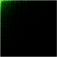
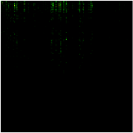
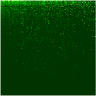
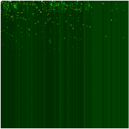
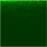
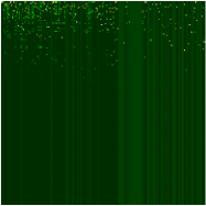
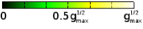
Figure 1: (Color online) Image of money mass matrix $M$ (top), Google matrix $G$ (middle) and inverse Google matrix $G^{*}$ (bottom) for all commodities (left column) and crude petroleum (right column) for year 2008 with all world countries $N=227$ from the UN COMTRADE comtrade . Matrix elements $g$, for $M_{i,j}$, $G_{i,j}$ or $G^{*}_{i,j}$, are shown by color changing from $0$ to a corresponding maximum value $g_{max}$. All three matrices are shown in the basis of PageRank index $K$ (and $K^{\prime}$) of matrix $G$, respectively for all commodities (left) and crude petroleum (right), which correspond to $x,y$-axis with $1\leq K,K^{\prime}\leq N$. Here we use $\alpha=0.5$ for matrix $G$ and its PageRank index $K$ and the same $\alpha$ for $G^{*}$.

The PageRank performs ranking determined by ingoing links putting at the top most known and popular nodes. However, in certain networks outgoing links also play an important role. Recently, on an example of procedure call network of Linux Kernel software, it was shown alik that a relevant additional ranking is obtained by taking the network with inverse link directions in the adjacency matrix corresponding to $A_{ij}\rightarrow A^{T}=A_{ji}$ and constructing from it an additional Google matrix $G^{*}$ according to relation (1) at the same $\alpha$. The examples of matrices $G$ and $G^{*}$ for the world trade network are shown in Fig. 1. The eigenvector of $G^{*}$ with eigenvalue $\lambda=1$ gives then a new inverse PageRank $P^{*}(i)$ with ranking index $K^{*}(i)$. This ranking was named CheiRank wiki to mark that it allows to chercher l’information in a new way. While the PageRank rates the network nodes in average proportionally to a number of ingoing links, the CheiRank rates nodes in average proportionally to a number of outgoing links. The results obtained in alik ; wiki confirm this proportionality with the exponent $\beta_{out}=1/(\gamma_{out}-1)$.

Since each node belongs both to CheiRank and PageRank vectors the ranking of information flow on a directed network becomes two-dimensional. While PageRank highlights how popular and known is a given node, CheiRank highlights its communication and connectivity abilities. The examples of Linux and Wikipedia networks show that the rating of nodes based on PageRank and CheiRank allows to perform information retrieval and to characterize network properties in a qualitatively new way alik ; wiki .

In this work we apply CheiRank and PageRank approach to the World Trade Network (WTN) using the enormous and detailed United Nations Commodity Trade Statistics Database (UN COMTRADE) comtrade . Using these data we analyze the world trade flows both in import and export for all commodities for all years 1962 - 2009 available there at SITC1 and HS96 databases. We also performed analysis for specific commodities taken from SITC Rev. 1 database, mainly for year 2008: crude petroleum (S1-33101, ”Crude petroleum”), natural gas (S1-3411, ”Gas, natural”), barley (S1-0430, ”Barley, unmilled”), cars (S1-7321, ”Passenger motor cars, other than buses”), food (S1-0, ”Food and live animals”), cereals (S1-04, ”Cereals and cereal preparations”). Their codes and official UN names are given in brackets. In few cases, when certain countries were non-reporting their export, we complemented the WTN data from the import database.

For a given year we extract from the UN COMTRADE money transfer (in USD) from country $j$ to country $i$ that gives us money matrix elements $M_{ij}$ (for all types of commodities noted above). These elements can be viewed as a money mass transfer from $j$ to $i$. In contrast to the adjacency matrix $A_{ij}$ of WWW, where all elements are only $0$ or $1$, here we have the case of weighted elements. This corresponds to a case when there are in principle multiple number of links from $j$ to $i$ and this number is proportional to USD amount transfer. Such a situation appears for rating of scientific journals bergstrom , Linux PCN alik and for Wikipedia English articles hyperlink network wiki , where generally there are few citations (links) from a given article to another one. In this case still the Google matrix is constructed according to the usual rules and relation (1) with $S_{ij}=M_{ij}/m_{j}$ and $S_{ij}=1/N$, if for a given $j$ all elements $M_{ij}=0$. Here $m_{j}=\sum_{i}M_{ij}$ is the total export mass for country $j$. The matrix $G^{*}$ is constructed from transposed money matrix with $S_{ij}=M_{ji}/\sum_{i}M_{ji}$. In this way we obtain the Google matrices $G$ and $G^{*}$ of WTN which allow to treat all countries on equal grounds independently of the fact if a given country is rich or poor. A similar choice was used in rating of scientific journals bergstrom , PCN Linux alik and Wikipedia network wiki . The main difference appearing for WTN is a very large variation of mass matrix elements $M_{ij}$ related to the fact that there is very strong variation of richness of various countries. Due to these reason we think that it is important to use the ranking based on the Google matrix which treats in a democratic way all world countries that corresponds to the democratic standards of the UN. For the WTN CheiRank and PageRank are naturally linked to export and import flows for a given country and hence it is very natural to use these ranks for characterization of country trade abilities. The Google matrix can be constructed in the same way not only for all commodities but also for a given specific commodity.

We note that recently the interest to the analysis of the world trade as a network becomes more and more pronounced with a few publications in this area garlaschelli ; vespignani ; benedictis ; hedeem . Thus, the global network characteristics were considered in garlaschelli ; vespignani , degree centrality measures were analyzed in benedictis and time evolution of network global characteristics was studied in hedeem . Topological and clustering properties of multinetwork of various commodities were discussed in garlaschelli2010 . Here we present a systematic study of directed WTN on the basis of new combination of PageRank and CheiRank methods using the Google matrix constructed for the enormous UN COMTRADE database.

The paper is composed as follows: in Section 2 we describe the global properties of the Google matrix of WTN, in Section 3 we analyze distribution of countries in PageRank-CheiRank plane for all time period 1962 - 2009 and propose a random matrix model of WTN (RMWTN) which describes the statistical properties of this distribution in the case of all commodities; comparison with ranking based on import and export for various commodities is presented in Section 4; discussion of the results is given in Section 5. More detailed information and data are given in Appendix and at the website cheirankpage .

2 Properties of Google matrix of WTN

An example of the Google matrix of WTN in 2008 is shown in Fig. 1 for all commodities and crude petroleum. The matrices $G$ and $G^{*}$ are shown in the bases where all countries are ordered by the PageRank index $K$ of matrix $G$ constructed for corresponding commodity (left and right columns). The matrix elements of $G$ are distributed over all $N$ values being roughly homogeneously in $K$, even if the left top corner at small $K$, $K^{\prime}$ values is filled in a more dense way. In contrast the density drops at large values of $K^{\prime}$. Such a structure is visible both for all commodities and crude petroleum but clearly the global density is smaller in the later case since there are less number of links there (see data in next Section). The structure of $G^{*}$ is approximately the same (we will see in next Section that rich countries are located at low $K$, $K^{\prime}$ values). In contrast to $G$ and $G^{*}$ the structure of money matrix $M$ is rather different. For all commodities matrix elements drop very rapidly at large values of $K$ and $K^{\prime}$ that corresponds to the fact that the main amount of world money circulates only between rich countries with top ranks $K$. In contrast to that for crude petroleum the matrix elements of $M$ are located at intermediate $K$ values. Indeed, in this case PageRank index $K$ orders countries by their crude petroleum trade where richest countries are not necessarily at the top ranks.

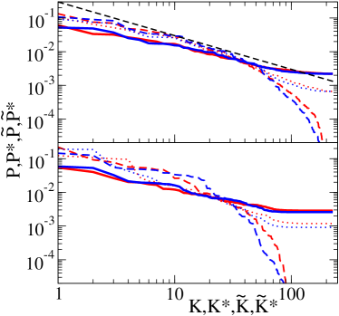
Figure 2: (Color online) Probability distributions of PageRank $P(K)$, CheiRank $P^{*}(K^{*})$, ImportRank $\tilde{P}(\tilde{K})$, and ExportRank $\tilde{P^{*}}(\tilde{K^{*}})$ are shown as function of their indexes in logarithmic scale for all commodities (top panel) and crude petroleum (bottom panel) for WTN in 2008 with $N=227$. Here $P(K)$ and $P^{*}(K^{*})$ are shown by red and blue curves respectively, for $\alpha=0.5$ (solid curves) and $\alpha=0.85$ (dotted curves); $\tilde{P}(\tilde{K})$ and $\tilde{P}^{*}(\tilde{K}^{*})$ are displayed by dashed red and blue curves respectively. For both commodities the distributions $P(K)$ and $P^{*}(K^{*})$ follow a power law dependence like $P\propto 1/K^{\beta}$ (see text), the Zipf law is shown by the straight dashed line with $\beta=1$ in top panel.

From the Google matrices $G$ and $G^{*}$ we find the probability distributions PageRank $P(K)$ and CheiRank $P^{*}(K^{*})$ which are shown in Fig. 2 for the same commodities as Fig. 1. One of the main features of these distributions is that both $P(K)$ and $P^{*}(K^{*})$ depend on their indexes in a rather similar way from, that is in contrast to the results found for the WWW donato ; upfal , PCN Linux alik and Wikipedia network wiki , where these distributions are different having different exponents $\beta$ in the power law decay. Here, up to fluctuations, we have $\beta_{in}=\beta_{out}=\beta$. The size of WTN is rather small compared to usual sizes of WWW, Linux or Wikipedia networks. However, still we find that the power law gives a quite good fit of our data. The fit gives $\beta=1.17\pm 0.015$ at $\alpha=0.85$ and $\beta=0.63\pm 0.01$ at $\alpha=0.5$ (for all commodities) and $\beta=0.92\pm 0.02$ and $\beta=0.51\pm 0.01$ respectively (for crude petroleum) for all 227 countries in Fig. 2. For the fit of top 100 countries we have respectively $\beta=1.15\pm 0.03$ ($\alpha=0.85$) and $\beta=0.75\pm 0.008$ ($\alpha=0.5$) for all commodities and $\beta=1.22\pm 0.015$ ($\alpha=0.85$) and $\beta=0.70\pm 0.008$ ($\alpha=0.5$) for crude petroleum. There is a certain change of the exponent with a decrease of the fit interval which, however, is not very large. We attribute this to visible deviations at the tail of $K$, $K^{*}$ with small countries (see discussion in next Section). In average the exponent value is not very far from the value $\beta=1$ corresponding to the Zipf law zipf .

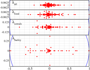
Figure 3: (Color online) Spectrum of the eigenvalues $\lambda$ of the Google matrix at $\alpha=1$ in complex plane for WTN in 2008 with $N=227$ countries for all commodities, food, cereals and barley (from top to bottom); all eigenvalues are shown for each commodity; unit radius circle is also shown. Only the bottom case have quasi-degenerate eigenvalues close to the circle with $3$ values $\lambda=1.,0.99987,0.991$ and two values close to $\lambda=-1$; other cases have a significant gap separation from $|\lambda|=1$.

It is useful to compare the behavior of probabilities $P(K)$ and $P^{*}(K^{*})$ with respective ranking related to import and export. To do that we rank the countries by probability import $\tilde{P}(\tilde{K})$ defined as a ratio of import in USD for a given country $\tilde{K}$ to the total world import in USD for a given year with ordering of all countries in decreasing probability order index of ImportRank $\tilde{K}$. By construction we have $\sum_{\tilde{K}}\tilde{P}(\tilde{K})=1$ and $\tilde{P}(\tilde{K})=m_{\tilde{K}}/M_{T}$, where $m_{\tilde{K}}$ is the import mass of a given country $\tilde{K}$ and $M_{T}=\sum_{i,j}M_{ij}$ is the total world money mass for a given year. In the same way we construct export probability $\tilde{P^{*}}(\tilde{K^{*}})$ with the ExportRank $\tilde{K^{*}}$. The dependence of these probabilities on their indexes is shown in Fig. 2. In the range of $1\leq\tilde{K},\tilde{K^{*}}\leq 50$ it can be well described by a power law with $\beta=1.01\pm 0.03$ for all commodities corresponding to the Zips law (for crude petroleum we obtain for this range $\beta=1.43\pm 0.07$). At larger values of order index we find a sharp drop with an exponential type decay on the tail. For crude petroleum this exponential decay starts at smaller values of $K$ due to a significantly smaller total number of links that gives an increase of $\beta$ for the range of 50 countries. The exponential decay at large $K$ results from a strong variation of richness of countries which changes more than by four orders of magnitude. From the comparison of ranks shown in Fig. 2 it is clear that PageRank and CheiRank give more equilibrated and democratic description of trade flows.

We should note that due to a small size of the WTN the fluctuations are stronger compared to large size networks like the WWW. It is especially visible for specific commodities where the total number of links is by factor 30 smaller then for all commodities (see next Section). These fluctuations are smaller for the damping factor value $\alpha=0.5$ in agreement with the results presented in avrachenkov ; ggs . In fact this $\alpha$ value was also used in redner for PhysRev citation network. Due to that reasons in next Sections we show data for ranking at $\alpha=0.5$.

Finally let us discuss the spectrum $\lambda$ of the Google matrix which follows from the equation for right eigenvectors $\psi_{m}(i)$:

$$\sum_{j}G_{ij}\psi_{m}(j)=\lambda_{m}\psi_{m}(i)\;\;.$$ (2)

It is known that the dependence on $\alpha$ is rather simple: all eigenvalues, except one with $\lambda=1$, are multiplied by $\alpha$ googlebook . Due to that we show the spectrum of $G$ at $\alpha=1$ in Fig. 3. Compared to the spectrum studied for other networks (see examples in alik ; ggs ; ulam1 ; ulam2 ; ulam3 ; weylinux ) we find that the WTN spectrum is very close to real line especially for three top commodities in Fig. 3. We explain this by the fact that here an average number of links per country is very large for these commodities and that the matrix elements are not very far from the symmetric relation $M_{ij}=M_{ji}$ at which the spectrum is real. We only note that for barley the spectrum has quasi-degeneracy at $\lambda=1$ that signifies the existence of slow relaxation modes. We attribute this to the fact that there are certain countries which practically do not use barley that leads to appearing of isolated subspaces with corresponding quasi-degenerate modes. We will return to the discussion of spectrum properties of $G$ in next Section.

3 CheiRank versus PageRank for WTN

We start from examples of distributions of countries in the PageRank-CheiRank plane shown in Fig. 4 for 5 different commodities in 2008. The first case of all commodities corresponds to trade flows between countries integrated over all type of products. Even if the Google matrix approach is based on a democratic ranking of international trade, being independent of total amount of export-import for a given country, we still find at the top ranks $K$ and $K^{*}$ the group of industrially developed countries (see more details in Table 1 in Appendix). This means that these countries have efficient trade networks with optimally distributed trade flows. Another pronounced feature of global distribution is that it is concentrated along the main diagonal $K=K^{*}$. This feature is not present in other networks studied before (e.g. PCN Linux alik and Wikipedia wiki ). The origin of this density concentration is based on simple economy reason: for each country the total import is approximately equal to export since each country should keep in average an economic balance. Thus for a given country its trade is doing well if its $K^{*}<K$ so that the country exports more than it imports. The opposite relation $K^{*}>K$ corresponds to a bad trade situation. We also can say that local minima in the curve of $(K^{*}-K)\;vs.\;K$ correspond to a successful trade while maxima mark bad traders. In 2008 most successful were China, Rep. of Korea, Russia, Singapore, Brasil, South Africa, Venezuela (in order of $K$ for $K\leq 50$) while among bad traders we note UK, Spain, Nigeria, Poland, Czech Rep., Greece, Sudan with especially strong export drop for two last cases. The comparison of our ranking with the import-export ranking will be analyzed in next Section.

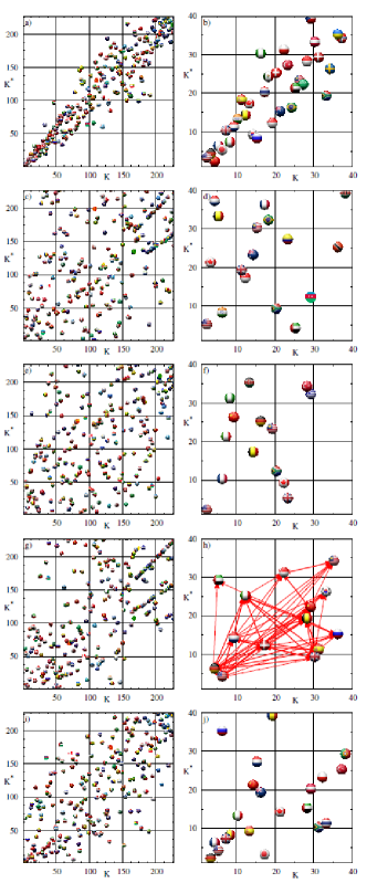
Figure 4: (Color online) Country positions in PageRank-CheiRank plane $(K,K^{*})$ for world trade in various commodities in 2008. Each country is shown by circle with its own flag (for a better visibility the circle center is slightly displaced from its integer position $(K,K^{*})$ along direction angle $\pi/4$). The panels show the ranking for trade in the following commodities: all commodities $(a,b)$; crude petroleum $(c,d)$; natural gas $(e,f)$; barley $(g,h)$; cars $(i,j)$. Left column shows a global scale with all 227 countries, while right column gives a zoom in the region of $40\times 40$ top ranks. For barley in panel (h) the links between countries inside the selected region are shown by arrows.

Even if there is a concentration of density along the main diagonal (Fig. 4a) we still have a significant broadening of distribution especially at middle values of $K\sim 100$. This means that the gravity model of trade, often used in economy (see e.g. krugman2011 ; benedictis ), has only approximate validity. Indeed, in this model the mass matrix $M_{ij}$ is symmetric that would placed all countries on diagonal $K=K^{*}$ that is definitely not the case.

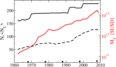
Figure 5: (Color online) Time evolution of the number of countries ($N$, full black curve), average number of links per country ($\langle N_{L}\rangle$) for all commodities (dashed curve) and crude petroleum (points for five years), total amount of money ($M_{T}=\sum_{i,j}M_{ij}$, red curve). The scale of $N$ and $\langle N_{L}\rangle$ is shown on left side, while $M_{T}$ values, in $\${\it USD}$, are given in logarithmic scale on the right side.

If we now turn to the distribution of countries for a trade in a specific commodity than it becomes absolutely clear that the symmetry approximately visible for all commodities is absolutely absent: the points are scattered practically over the whole square $N\times N$. The reason of such a strong scattering is clear: e.g. for crude petroleum some countries export this product while other countries import it. Even if there is some flow from exporters to exporters it remains relatively low (see more discussion in next Section). This makes the Google matrix to be very asymmetric. Indeed, the asymmetry of trade flow is well visible in Fig. 4h where arrows show the trade directions between countries within top $40\times 40$ ranks for barley.

It is also useful to use 2DRank $K_{2}$ discussed in wiki , which orders all nodes according to the order of their appearance inside squares of size $K\times K$ going from $K=1,2,3,...$ to $N$ for each of four specific commodities shown in Fig. 4. In a certain sense top countries in 2DRank $K_{2}$ are those which are active traders even not being among large exporters or importers of this product (all ranks for commodities of Fig. 4 are given in Tables 1-5 in Appendix). As an example, we note Singapore which is at the third position in $K_{2}$ (Table 2): it is a small country which cannot export or import a large amount of the commodity, but its trade network is very active redistributing flows between various countries that places it at a high $K_{2}$ rank.

The images of Fig. 4 allow to understand qualitatively the reasons of density concentration around diagonal $K=K^{*}$ for the case of all commodities: this trade is composed from hundreds of specific commodities which behave randomly and the averaging over them gives effective coarse-graining and produces a certain symmetry for matrix elements due to the central limit theorem for a sum of many positive contributions. The fact that the increase of coarse-graining cell gives more and more symmetry is well seen in Fig. 3 where the spectrum becomes more and more close to a real one, and hence there is more and more symmetry in elements $G_{ij}$, when we go from barley to cereals, food and all commodities.

We will return to the analysis of specific country ranking in the next Section while now we turn to analysis of time evolution of WTN.

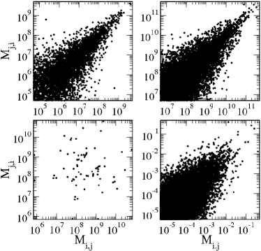
Figure 6: Money mass transfer matrix elements $M_{i,j}$ are shown versus their transposed values $M_{j,i}$ for all commodities of WTN in 1962 (top left panel) and 2008 (top right panel). Bottom left panel shows the matrix elements for crude petroleum of WTN in 2008; bottom right panel shows the same quantities for random matrix model of WTN. Four panels show 5 orders of magnitude in logarithmic scales starting from maximum values of $M_{ij}$. In the case of WTN (top and bottom left panels) matrix elements are taken from the UN COMTRADE database and are expressed in USD, right bottom panel is built from one random realization with $M_{ij}=\epsilon_{i}\epsilon_{j}/ij$ (see text). Here $N=164$ for 1962 data; $N=227$ for 2008 data and RMWTN.

The variation of global parameters of WTN during the database period 1962 - 2009 is shown in Fig. 5. The number of countries is increased by 38%, while the number of links per country for all commodities is increased in total by 140% with a significant increase from 50% to 140% during the period 1993 - 2009 corresponding to economy globalization. At the same time for a specific commodity the average number of links per country remains on a level of 3-5 links being by a factor 30 smaller compared to all commodities trade. During the whole period the total amount $M_{T}$ of trade in USD shows an average exponential growth by 2 orders of magnitude.

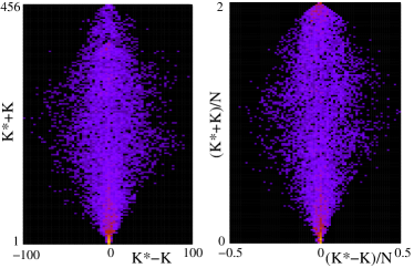
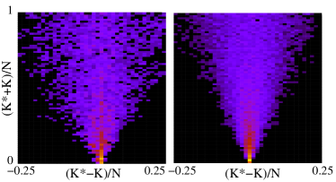
Figure 7: (Color online) Spindle distribution for WTN of all commodities for all countries in the period 1962 - 2009 shown in the plane of $(K^{*}-K,K^{*}+K)$ (left top panel, coarse-grained data in $3\times 3$ cell size) and in the rescaled plane $((K^{*}-K)/N,(K^{*}+K)/N)$ (right top panel, coarse-graining inside each of $76\times 152$ cells, which is approximately the same number as in top left panel); data from the UN COMTRADE database. Bottom left panel: zoom of top right panel; bottom right panel: data from 100 realisations of RMWTN model (3) with $N=227$ as for WTN size in 2008.

To understand the physical properties of the WTN we consider the distribution of money mass transfer matrix elements $M_{ij}$ shown versus their transposed values $M_{ji}$ in Fig. 6. This distribution is symmetric by the construction. In the case of symmetric matrix $M_{ij}$, corresponding to the gravity model of trade or undirected network, all elements should be located on one diagonal line that is definitely not the case. For crude petroleum the distribution is even more broad showing definite absence of symmetry of $M_{ij}$. In fact for all commodities the distribution forms a rather broad cone which form remains stable in time according to the comparison of data in 1962 and 2008 years (the density is higher in the later case since there are more countries). Keeping in mind that according to data of Fig. 2 we have the Zipf law for $\tilde{P}(\tilde{K})$ we propose the random matrix model of WTN (RMWTN) with the mass matrix elements given by

$$M_{ij}=\epsilon_{i}\epsilon_{j}/ij\;\;,$$ (3)

where $\epsilon_{i}$ are random numbers homogeneously distributed in $[0,1]$ interval and $i,j$ are indexes in the ImportRank index $\tilde{K}$. The distribution given by this simple model reproduces quite well the actual distribution found for all commodities (see right panels in Fig. 6). With this RMWTN distribution of $M_{ij}$ we construct the Google matrices $G$ and $G^{*}$ according to the usual recipes (1) and then determine the distribution of points in $(K,K^{*})$ plane.

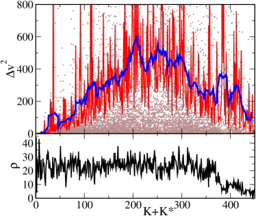
Figure 8: (Color online) Top panel shows velocity square $\Delta v^{2}$ as a function of $K+K^{*}$ for all countries and all years (all commodities data). Gray circles represent all values of $\Delta v^{2}$, red curve shows the value of $\Delta v^{2}$ averaged over cases with fixed $K+K^{*}$, blue curve shows the average of the red curve data in the interval $[K+K^{*}-10,K+K^{*}+10]$. In the bottom panel the number of cases $\rho(K+K^{*})$ at a given $K+K^{*}$ is shown as a function of $K+K^{*}$.

To have a statistical comparison between the RMWTN and real WTN data we construct the density distribution of countries in the plane $(K^{*}-K,K^{*}+K)$ using all available years 1962 - 2009 at the UN COMTRADE database for all commodities. The coarse-grained distribution of about $10^{4}$ WTN data points is shown in Fig. 7. We present the data directly in $(K^{*}-K,K^{*}+K)$ plane (top left panel) and in rescaled variables $((K^{*}-K)/N,(K^{*}+K)/N)$ plane, which takes into account that the number of countries grown by 38% during this time period. The distribution has a form of spindle with maximum density at the vertical axis $K^{*}-K=0$. We remind that good exporters are on the left side of this axis at $K^{*}-K<0$, while the good importers (bad exporters) are on the right side at $K^{*}-K>0$.

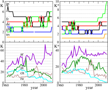
Figure 9: (Color online) Time evolution of CheiRank and PageRank indexes $K$, $K^{*}$ for some selected countries for all commodities. The countries shown in top panels are: Japan (jp-black), France (fr-red), Fed. Rep. of Germany and Germany (de - both in blue), Great Britain (gb - green), USA (us - orange) [curves from top to bottom in 1962 in left top panel]. The countries shown in bottom panels are: Argentina (ar - violet), India (in - dark green), China (cn - cyan), USSR and Russian Fed. (ru - both in gray) [curves from top to bottom in 1975 in left bottom panel].

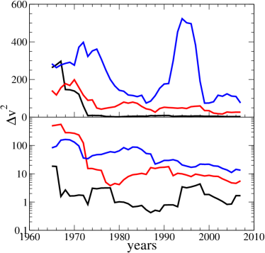
Figure 10: (Color online) Time evolution of velocity square $\Delta v^{2}$ for all commodities averaged over five years interval. In addition $\Delta v^{2}$ is averaged over countries in the following intervals: $1\leq K+K^{*}\leq 40$ (blue curve), $41\leq K+K^{*}\leq 80$ (red curve), $81\leq K+K^{*}\leq 120$ (black curve) in top panel; $1\leq K+K^{*}\leq 20$ (blue curve), $21\leq K+K^{*}\leq 40$ (red curve), $41\leq K+K^{*}\leq 60$ (black curve) in bottom panel.

The comparison of WTN data with the results produced by RMWTN model (3) are shown in bottom panels of Fig. 7: there is a good agreement between both without any fit parameters for the half of all countries with top ranks ($K+K^{*}<N$). For countries with $K+K^{*}>N$ the RMWTN model does not succeed to describe correctly the upper part of spindle distribution found for the WTN and hence further improvements of the RMWTN are needed. However, a simple description of the distribution for a half top countries is rather successful.

A remarkable feature of the WTN spindle distribution of Fig. 7 (top right) is the appearance of high density domains at $K^{*}-K\approx 0$ with $K+K^{*}\approx 1$ and $K+K^{*}\approx 2N$. They give an impression of two solid phases emerging in these two regions while the other part looks like a gas phase. This view gets additional confirmation by data of Fig. 8 where we present the velocity square $(\Delta v)^{2}$, averaged over the whole period 1962 - 2009, as a function of $K+K^{*}$. This local quantity is defined as $(\Delta v)^{2}=(K(t1)-K(t-1))^{2}+(K^{*}(t)-K^{*}(t-1))^{2}$ via a one year displacement of a given country in $(K,K^{*})$ plane with further averaging over all times and all countries. These data clearly show that for $K+K^{*}\leq 20$ we have very small square velocity (small effective temperature) corresponding to a solid phase of rich countries, while for $K+K^{*}>20$ we have large square velocity (large effective temperature) corresponding to a gas phase with rapid rank fluctuations. There is a similar visible drop of temperature at another limit of most poor countries with $K+K^{*}\approx 2N$ which indicates a formation of solid phase of poor countries (the data are not so exact for this region due to variation of number of UN countries with time).

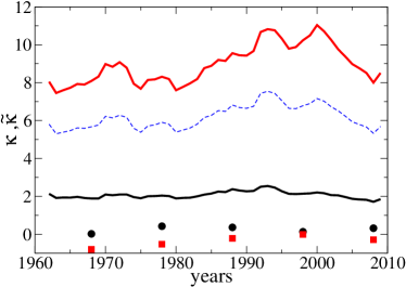
Figure 11: (Color online) Time evolution of correlators of PageRank–CheiRank ($\kappa$) and ImportRank–ExportRank ($\tilde{\kappa}$). All commodities are shown by solid red curve for $\tilde{\kappa}$, and solid black curve and dashed blue curve for $\kappa$ with $\alpha=0.5$ and $\alpha=0.85$ respectively. Correlators for crude petroleum with 10 years of separation are shown in red squares for $\tilde{\kappa}$ and black circles for $\kappa$.

The presence of solid phase of rich countries and gas phase of other countries is also visible from analysis of rank variation in time for individual countries shown in Fig. 9: for $K,K^{*}\leq 10$ the curves are almost flat while for $K,K^{*}>10$ we see strong fluctuation of curves. It is interesting to note that sharp increases in $K$ mark crises in 1991, 1998 for Russia and in 2001 for Argentina (import is reduced in period of crises). We also see that in recent years the solid phase is perturbed by entrance of new countries like China and India. However, the results presented in Fig. 10 for the variation of square velocity with time for three regions of $K+K^{*}$ show that the top 10, and even top 20, countries have rather small velocities $\Delta v^{2}$, compared to those with $(K+K^{*})/2\approx K>20$. For $K\leq 20$ we have $\Delta v^{2}$ which remains constant in time. In a certain sense it looks that the countries with $20<K<40$ protect those with $1\leq K\leq 20$ (approximately corresponding to G-20 major economies g20 ), so that their temperature at $1\leq K\leq 20$ remains unaffected even by a very larger fluctuation well visible for the range $81\leq K+K^{*}\leq 120$ during the period of 1992 - 1998 with a few financial crises of Black Wednesday, Mexico crisis, Asian crisis and Russian crisis.

The presented results for distribution of countries and analysis of their time evolution in the PageRank-CheiRank plane confirm a well known statement that “the poor stay poor and the rich stay rich”.

Finally let us discuss an additional parameter which characterizes the correlation between PageRank and CheiRank vectors. The correlator between PageRank and CheiRank is defined as

$$\kappa=N\sum_{i}P(K(i))P^{*}(K^{*}(i))-1\;,$$ (4)

and in a similar way the correlator between ImportRank and ExportRank is given by

$$\tilde{\kappa}=N\sum_{i}\tilde{P}(\tilde{K}(i))\tilde{P}^{*}(\tilde{K}^{*}(i))-1\;.$$ (5)

Recently it has been found that there are networks with small correlator, like PCN Linux alik , and large correlator, as Wikipedia wiki . Here we find that for all commodities we have large values of $\kappa$ and $\tilde{\kappa}$, which have rather similar dependence on time (see Fig. 11). In contrast, there are almost zero or even negative correlations for crude petroleum. Indeed, for crude petroleum there is no correlation between export and import while for all commodities they are strongly correlated.

4 Comparison with Import - Export ranking

It is important to compare rating based on PageRank and CheiRank with the useful way of country rating based on ImportRank and ExportRank (see e.g cia2010 ). With this aim we present the distribution of country positions on the planes $(\tilde{K},K)$ and $(\tilde{K^{*}},K^{*})$ shown for top 100 for the same commodities as in Fig. 4 for year 2008. For all commodities there is a clear correlation between PageRank and ImportRank since the distribution of points is centered along the diagonal $K=\tilde{K}$. It starts to spread only around $K\approx\tilde{K}\approx 30$. At the same time for CheiRank and ExportRank such a spreading from diagonal starts significantly earlier at $\tilde{K^{*}}\approx K^{*}\approx 10$.

For other commodities shown in Fig. 12 the correlations between ranking based on Google matrix and corresponding Export or/and Import ranking are practically absent showing very broad scattering of points around almost the whole plane. Only for cars there is a certain level of correlation for approximately the first 10 ranks. Natural products like crude petroleum, natural gas and agriculture products like barley show no correlations.

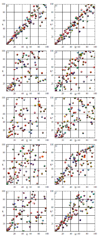
Figure 12: (Color online) Comparison of ranking between PageRank $K$ and ImportRank $\tilde{K}$ (left column), and between CheiRank $K^{*}$ and ExportRank $\tilde{K}^{*}$ (right column) for year 2008. The shown commodities are: all commodities (panels a, b); crude petroleum (panels c, d); natural gas (panels e, f); barley (panels g, h); cars (panels i, j). Only top 100 ranks are shown.

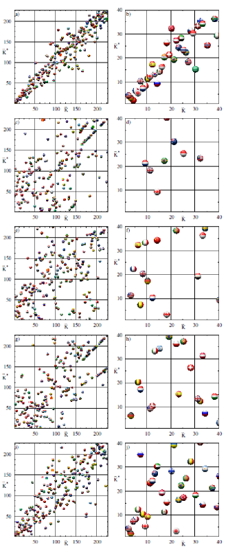
Figure 13: (Color online) Country positions in the ImportRank-ExportRank plane $(\tilde{K},\tilde{K}^{*})$ for year 2008. The shown commodities are: all commodities (panels a, b); crude petroleum (panel c, d); natural gas (panel e, f); barley (panel g, h); cars in i) and j). Left column shows a global scale (227 countries) while right column illustrates the first $40\times 40$ region. Data can be compared with those in Fig. 4.

The similar conclusions can be also drawn from the comparison of country distributions in the plane $(K,K^{*})$ (Fig. 4) and in the plane $(\tilde{K},\tilde{K}^{*})$ (Fig. 13), which show data on the same scales. Clearly, the distributions are rather different and only for all commodities we can see visible correlations (we note that appearance of ordered short line segments in panels (c,g) around $K\approx\tilde{K}\approx 200$ is due to degeneracy of $P$ and $\tilde{P}$ values, for those countries which e.g. do not use barley, and thus their ordering becomes somewhat arbitrary).

Let us discuss in more detail few concrete examples shown in Tables 1-5 in Appendix. For all commodities first 5 positions are very close in both ways of ranking. As a significant change we note Canada which moves from $\tilde{K}^{*}=11$ down to $K^{*}=16$ and Mexico with respective change from $\tilde{K}^{*}=13$ to $K^{*}>20$: the export of these two countries is too strongly oriented on USA that becomes directly visible through CheiRank analysis. In contrast Singapore moves up from $\tilde{K}^{*}=15$ to $K^{*}=11$ that shows the stability and broadness of its export trade, a similar situation appears for India moving up from $\tilde{K}^{*}=19$ to $K^{*}=12$.

Even more strong changes of ranking appear for specific commodities. For example for crude petroleum Russia moves up from $\tilde{K}^{*}=2$ to $K^{*}=1$ showing that its trade network in this product is better and broader than the one of Saudi Arabia. Iran moves in opposite direction from $\tilde{K}^{*}=5$ down to $K^{*}=14$ showing that its trade network is restricted to a small number of nearby countries. A significant improvement of ranking takes place for Kazakhstan moving up from $\tilde{K}^{*}=12$ to $K^{*}=2$. The direct analysis shows that this happens due to an unusual fact that Kazakhstan is practically the only country which sells crude petroleum to the CheiRank leader in this product Russia. This puts Kazakhstan on the second position. It is clear that such direction of trade is more of political or geographical origin and is not based on economic reasons.

For natural gas there are also significant differences between two ways of ranking. Thus, USA moves strongly up from $\tilde{K}^{*}=10$ to $K^{*}=1$ due its broad trade network in this product. Canada moves down from $\tilde{K}^{*}=2$ to $K^{*}=8$ due to its too strong trade orientation on USA. A small country Trinidad and Tobago moves up from $\tilde{K}^{*}=15$ to $K^{*}=2$ since it provides about 70% of import of top leader USA.

Significant reordering appears also for barley trade. Thus, the leader Ukraine moves down from $\tilde{K}^{*}=1$ to $K^{*}=6$ due to too narrow trade network and USA moves up from $\tilde{K}^{*}=8$ to $K^{*}=3$ due to its broad trade network.

For trade of cars we have France going up from $\tilde{K}^{*}=7$ to $K^{*}=3$ due to its broad export network. Also Thailand goes strongly up from $\tilde{K}^{*}=19$ to $K^{*}=10$ due to its broad trade links. We note that on the side of import we have strong change for Nigeria which moves from $\tilde{K}>20$ up to $K=1$. This is the most populated country in Africa with a strong income due to oil trade which provides a large fraction of USA import. With such oil income Nigeria buys cars from all over the world and thus becomes at the top of PageRank.

Finally we note that among top 20 countries ranked in 2DRank $K_{2}$ by all commodities in 2008 (see Table 1) there 14 among G-20 major economies g20 . At the same time ExportRank gives 13, and ImportRank gives 14 countries from 19 of G-20-list. We attribute a difference in 5 countries to political and geographical aspects of G-20-selection.

5 Discussion

In this work we constructed the Google matrix of the WTN using the enormous UN COMTRADE database. From this matrix we obtained PageRank and CheiRank of all world countries in various types of trade products for years 1962 - 2009. This new approach gives a democratic type of ranking being independent of the trade amount of a given country. In this way rich and poor countries are treated on equal democratic grounds. In a certain sense PageRank probability for a given country is proportional to its rescaled import flows while CheiRank is proportional to its rescaled export flows inside of the WTN.

The global characteristics of the world trade are analyzed on the basis of this new type of ranking. Even if all countries are treated now on equal democratic grounds still we find at the top rank the group of industrially developed countries approximately corresponding to G-20 (74%). Our studies establish the existence of two solid state domains of rich and poor countries which remain stable during the years of consideration. Other countries correspond to a gas phase with ranking strongly fluctuating in time. We propose a simple random matrix model which well describes the statistical properties of rank distribution for the WTN.

The comparison between usual ImportRank–ExportRank (see e.g. cia2010 ) and our PageRank–CheiRank approach shows that the later highlights the trade flows in a new useful manner which is complementary to the usual analysis. The important difference between these two approaches is due to the fact that ImportRank–ExportRank method takes into account only global amount of money exchange between a country and the rest of the world while PageRank–CheiRank approach takes into account all links and money flows between all countries. We hope that this new approach based on the Google matrix will find further useful applications to investigation of various flows in trade and economy.

Acknowledgments: We thank Gilles Saint-Paul (TSE, Toulouse) for useful discussions on economics and Olga Chepelianskaia (UN Bangkok) for insights on UN databases. Our special thanks are addressed to Arlene Adriano and Matthias Reister (United Nations Statistics Division) for provided help and friendly access to the UN COMTRADE database comtrade .

6 Appendix

Table 1: Top 20 ranking for all commodities – 2008.

Ran	$K$	$K^{*}$	$K_{2}$	$\tilde{K}$	$\tilde{K}^{*}$
1	USA	China	USA	USA	China
2	Germany	USA	China	Germany	Germany
3	China	Germany	Germany	China	USA
4	France	Japan	Japan	France	Japan
5	Japan	France	France	Japan	France
6	UK	Italy	Italy	UK	Netherlands
7	Italy	Russian Fed.	UK	Netherlands	Italy
8	Netherlands	Rep. of Korea	Netherlands	Italy	Russian Fed.
9	India	UK	India	Belgium	UK
10	Spain	Netherlands	Rep. of Korea	Canada	Belgium
11	Belgium	Singapore	Belgium	Spain	Canada
12	Canada	India	Russian Fed.	Rep. of Korea	Rep. of Korea
13	Rep. of Korea	Belgium	Canada	Russian Fed.	Mexico
14	Russian Fed.	Australia	Spain	Mexico	Saudi Arabia
15	Nigeria	Brazil	Singapore	Singapore	Singapore
16	Thailand	Canada	Thailand	India	Spain
17	Mexico	Spain	Australia	Poland	Malaysia
18	Singapore	South Africa	Brazil	Switzerland	Brazil
19	Switzerland	Thailand	Mexico	Turkey	India
20	Australia	U. Arab Emir.	U. Arab Emir.	Brazil	Switzerland

Table 2: Top 20 ranking for crude petroleum – 2008.

Ran	$K$	$K^{*}$	$K_{2}$	$\tilde{K}$	$\tilde{K}^{*}$
1	USA	Russian Fed.	USA	USA	Saudi Arabia
2	Canada	Kazakhstan	India	Japan	Russian Fed.
3	Netherlands	U. Arab Emir.	Singapore	China	U. Arab Emir.
4	Belgium	USA	UK	Italy	Nigeria
5	India	Ecuador	South Africa	Rep. of Korea	Iran
6	China	Saudi Arabia	Canada	India	Venezuela
7	Germany	India	Australia	Germany	Norway
8	Japan	South Africa	U. Arab Emir.	Netherlands	Canada
9	Rep. of Korea	Nigeria	Colombia	France	Angola
10	UK	Sudan	Azerbaijan	UK	Iraq
11	Singapore	Azerbaijan	Malaysia	Spain	Libya
12	Italy	Venezuela	Brazil	Singapore	Kazakhstan
13	Australia	Norway	Belgium	Canada	Kuwait
14	Malaysia	Iran	Trinidad and Tobago	Thailand	Azerbaijan
15	Spain	Algeria	France	Belgium	Algeria
16	France	Singapore	Netherlands	Brazil	Mexico
17	Brazil	Kuwait	Kenya	Turkey	UK
18	Sweden	UK	Angola	South Africa	Qatar
19	South Africa	Angola	China	Poland	Oman
20	Thailand	Canada	Thailand	Australia	Netherlands

Table 3: Top 20 ranking for natural gas – 2008.

Ran	$K$	$K^{*}$	$K_{2}$	$\tilde{K}$	$\tilde{K}^{*}$
1	USA	USA	USA	Japan	Norway
2	Japan	Trinidad and Tobago	France	USA	Canada
3	Rep. of Korea	Norway	Belgium	France	Algeria
4	Spain	UK	South Africa	Rep. of Korea	Russian Fed.
5	France	Russian Fed.	Italy	Spain	Qatar
6	Italy	Oman	Canada	Belgium	Belgium
7	Nigeria	Australia	UK	UK	Indonesia
8	China	Canada	Malaysia	Italy	Malaysia
9	Poland	France	Germany	Germany	Netherlands
10	Portugal	Algeria	China	Ukraine	USA
11	El Salvador	South Africa	Nigeria	Netherlands	Australia
12	Kenya	Kazakhstan	Greece	Mexico	Nigeria
13	Belgium	Qatar	Turkey	China	Saudi Arabia
14	Guatemala	Saudi Arabia	Kenya	India	U. Arab Emir.
15	Germany	U. Arab Emir.	Netherlands	Hungary	Trinidad and Tobago
16	Mexico	Belgium	Rep. of Korea	Czech Rep.	Germany
17	Ecuador	Pakistan	Spain	Canada	Oman
18	Malaysia	Singapore	Russian Fed.	Brazil	Egypt
19	South Africa	Netherlands	India	Turkey	UK
20	Slovenia	Italy	Japan	Thailand	Turkmenistan

Table 4: Top 20 ranking for barley – 2008.

Ran	$K$	$K^{*}$	$K_{2}$	$\tilde{K}$	$\tilde{K}^{*}$
1	Saudi Arabia	France	USA	Saudi Arabia	Ukraine
2	Yemen	Canada	Germany	Germany	France
3	Germany	USA	Netherlands	Japan	Australia
4	U. Arab Emir.	Australia	Denmark	China	Canada
5	USA	Germany	Italy	Belgium	Germany
6	Israel	Ukraine	Belgium	Netherlands	Russian Fed.
7	Japan	Rep. of Moldova	China	Syria	Argentina
8	Netherlands	UK	U. Arab Emir.	Iran	USA
9	Oman	Argentina	UK	Jordan	Denmark
10	Greece	Spain	Spain	USA	Kazakhstan
11	Italy	Denmark	Singapore	Denmark	Romania
12	Croatia	Kazakhstan	Rep. of Korea	Italy	UK
13	Syria	Netherlands	Malaysia	Tunisia	Hungary
14	Kuwait	Russian Fed.	Russian Fed.	Israel	Spain
15	Cyprus	India	Austria	Colombia	Bulgaria
16	Denmark	Hungary	Poland	Algeria	Netherlands
17	Occ. Palestinian Terr.	Romania	Brazil	Kuwait	Lithuania
18	Switzerland	Belgium	Ireland	Brazil	Sweden
19	Bosnia Herzegovina	Lithuania	France	Morocco	Belgium
20	Jordan	Sweden	South Africa	Turkey	India

Table 5: Top 20 ranking for cars – 2008.

Ran	$K$	$K^{*}$	$K_{2}$	$\tilde{K}$	$\tilde{K}^{*}$
1	Nigeria	Germany	Germany	USA	Germany
2	Germany	Japan	USA	Germany	Japan
3	France	USA	France	UK	USA
4	USA	Rep. of Korea	UK	France	Canada
5	Russian Fed.	France	Belgium	Italy	Rep. of Korea
6	UK	UK	Spain	Russian Fed.	UK
7	Belgium	Belgium	Italy	Belgium	France
8	Ukraine	Spain	Japan	Canada	Spain
9	Italy	South Africa	Australia	Spain	Belgium
10	Greece	Thailand	Canada	China	Mexico
11	Venezuela	Mexico	China	Netherlands	Italy
12	Spain	Italy	Netherlands	Australia	Slovakia
13	China	Canada	U. Arab Emir.	U. Arab Emir.	Czech Rep.
14	Netherlands	U. Arab Emir.	Austria	Saudi Arabia	Poland
15	Australia	Czech Rep.	South Africa	Austria	Sweden
16	Japan	Slovakia	Poland	Mexico	Turkey
17	Albania	Hungary	Thailand	Poland	Hungary
18	Romania	Australia	Russian Fed.	Switzerland	Austria
19	Sudan	Austria	Turkey	Finland	Thailand
20	Canada	China	Portugal	Ukraine	South Africa

References

- (1) United Nations Commodity Trade Statistics Database http://comtrade.un.org/db/
- (2) P.R. Krugman, M. Obstfeld, M. Melitz, International economics: theory & policy, Prentic Hall, New Jersey (2011).
- (3) Central Intelligence Agency, The CIA Wold Factbook 2010, Skyhorse Publ. Inc. (2009)
- (4) S. Brin and L. Page, Computer Networks and ISDN Systems 30, 107 (1998).
- (5) A. M. Langville and C. D. Meyer, Google’s PageRank and Beyond: The Science of Search Engine Rankings, Princeton University Press (Princeton, 2006).
- (6) N. Litvak, W.R.W. Scheinhardt, and Y. Volkovich, Lecture Notes in Computer Science, 4936, 72 (2008).
- (7) D. Donato, L. Laura, S. Leonardi and S. Millozzi, Eur. Phys. J. B 38, 239 (2004).
- (8) G. Pandurangan, P. Raghavan and E. Upfal, Internet Math. 3, 1 (2005).
- (9) S. Redner, Physics Today 58, 49 (2005).
- (10) F. Radicchi, S. Fortunato, B. Markines, and A. Vespignani, Phys. Rev. E 80, 056103 (2009).
- (11) J. West, T. Bergstrom and C.T. Bergstrom, arXiv:0911.1807 (to appear in J. American Soc. Info. Sci. Tech. (2011)); http://eigenfactor.org/
-
(12)
A. D. Chepelianskii,
Towards physical laws for software architecture,
arXiv:1003.5455[cs.SE] (2010);
http://www.quantware.upstlse.fr/QWLIB/linuxnetwork/ - (13) A.O. Zhirov. O.V. Zhirov and D.L.Shepelyansky, Eur. Phys. J. B 77, 523 (2010); http://www.quantware.ups-tlse.fr/QWLIB/2drankwikipedia/
- (14) D. Garlaschelli and M.I. Loffredo, Physica A: Stat. Mech. Appl. 355, 138 (2005).
- (15) M.A. Serrano, M. Boguna and A. Vespignani, J. Econ. Interac. Coor. 2, 111 (2007).
- (16) L. De Benedictis and L. Tajoli, The World Trade Network, working paper (2009); available at http://www.eief.it/files/2010/10/luca-de-benedictis.pdf
- (17) J. He and M.W. Deem, Phys. Rev. Lett. 105, 198701 (2010).
- (18) M. Barigozzi, G. Fagiolo and D. Garlaschelli, Phys. Rev. E 81, 046104 (2010).
-
(19)
http://www.quantware.ups-tlse.fr/QWLIB/
tradecheirank/ - (20) G.K. Zipf, Human Behavior and the Principle of Least Effort, Addison-Wesley, Boston (1949).
- (21) K. Avrachenkov, N. Litvak and K. Pham, Internet Math. 5, 47 (2005).
- (22) B.Georgeot, O.Giraud and D.L.Shepelyansky, Phys. Rev. E 81, 056109 (2010).
- (23) D.L.Shepelyansky and O.V.Zhirov, Phys. Rev. E 81, 036213 (2010).
- (24) L.Ermann and D.L.Shepelyansky, Phys. Rev. E 81, 036221 (2010).
- (25) L.Ermann and D.L.Shepelyansky, Eur. Phys. J. B 75, 299 (2010).
- (26) L.Ermann, A.D. Chepelianskii and D.L.Shepelyansky, Eur. Phys. J. B 79, 115 (2011).
- (27) Wikipedia contributors. G-20 major economies. Wikipedia, The Free Encyclopedia, Web. 25 Mar. 2011.