Bounding the scalar dissipation scale for mixing flows in the presence of sources

Abstract

We investigate the mixing properties of scalars stirred by spatially smooth, divergence-free flows and maintained by a steady source-sink distribution. We focus on the spatial variation of the scalar field, described by the dissipation wavenumber, $k_{d}$, that we define as a function of the mean variance of the scalar and its gradient. We derive a set of upper bounds that for large Péclet number ($\text{Pe}\gg 1$) yield four distinct regimes for the scaling behaviour of $k_{d}$, one of which corresponds to the Batchelor regime. The transition between these regimes is controlled by the value of Pe and the ratio $\rho=\ell_{u}/\ell_{s}$, where $\ell_{u}$ and $\ell_{s}$ are respectively, the characteristic lengthscales of the velocity and source fields. A fifth regime is revealed by homogenization theory. These regimes reflect the balance between different processes: scalar injection, molecular diffusion, stirring and bulk transport from the sources to the sinks. We verify the relevance of these bounds by numerical simulations for a two-dimensional, chaotically mixing example flow and discuss their relation to previous bounds. Finally, we note some implications for three dimensional turbulent flows.

1 Introduction

Mixing of scalar fields is a problem that is crucial to several environmental issues as well as engineering applications. In many situations the underlying flow is spatially smooth and divergence-free while molecular diffusion is usually much weaker than the stirring strength of the flow (see e.g. Aref (2002)). Notwithstanding the apparent simplicity of the flow, its effect on the scalar field can be rather complex: A simple time-dependence is often sufficient for the flow to be chaotically mixing in which case the gradients of the scalar fields are greatly amplified (Aref (1984); Ottino (1989); Ott (1993)). Batchelor (1959) recognized that this amplification is responsible for the rapid dissipation of any initial scalar inhomogeneity and thus the efficiency at which a scalar is mixed.

In the continual presence of sources and sinks, a statistical equilibrium is attained in which the rate of injection of scalar variance balances the rate of its dissipation. In this case, the most basic way to measure the flow’s mixing efficiency is to consider the equilibrium variance of the scalar: the lower its value, the better mixed is the scalar field. Thiffeault et al. (2004) derived a rigorous lower bound for the scalar variance that was further enhanced by Plasting & Young (2006) using the scalar dissipation rate as a constraint. Doering & Thiffeault (2006) and Shaw et al. (2007) derived bounds for the small- and large-scale scalar variance (respectively measured by the variance of the gradient $\langle|\nabla\theta|^{2}\rangle$ and the anti-gradient $\langle|\nabla^{-1}\theta|^{2}\rangle$ of the scalar field $\theta$, where $\langle\cdot\rangle$ denotes a space-time average defined in equation (2)). This set of bounds have successfully captured some of the key parameters in the flow and source-sink distribution that control the scalar variances. Their general applicability means that they can be used to test theoretical predictions of scalar mixing for various flow and source-sink configurations. This is especially useful for high-Péclet flows ($\text{Pe}\gg 1$) for which analytical solutions are difficult to obtain while high-resolution numerical simulations can become prohibitively expensive. However, the bounds on the variance of the scalar and its gradient do not depend on the gradients of the velocity field and in many cases, can be realized by uniform flows. They therefore do not capture the effect of stirring. These bounds are then relevant when the mixing of a scalar is mainly controlled by the process of transport from the sources to the sinks.

Motivated by the apparent lack of control of the stirring process, we here focus on the characteristic lengthscale, $\ell_{d}$, at which the scalar variance is dissipated, or equivalently its inverse, the dissipation wavenumber, $k_{d}\equiv\ell_{d}^{-1}$. Its value, should, within a suitable range of parameters, be directly related to the Batchelor lengthscale, $\ell_{{}_{B}}$. The latter lengthscale, obtained in Batchelor (1959), describes the effect of stirring on the spatial structure of the scalar field.

We here examine the behaviour of $k_{d}$ for different values of the control parameters, Pe and $\rho$, where $\rho$ denotes the ratio of the characteristic lengthscale of the velocity, $\ell_{u}$, and that of the source field, $\ell_{s}$. After formulating the problem in section 2, we next seek a set of upper bounds for $k_{d}$ (section 3). In section 4, we investigate the behaviour of these bounds as $\rho$ varies. We find that, in the high-Péclet limit, the behaviour of $k_{d}$ is characterized by four distinct regimes, one of which corresponds to the Batchelor regime. The use of homogenization theory implies a fifth regime for $k_{d}$. In section 5, we examine the relevance of the bounds by performing a set of numerical simulations for a renewing type of flow. We conclude in section 6.

2 Problem formulation

The temporal and spatial evolution of the concentration, $\theta(\bm{x},t)$, of a passive scalar, continually replenished by a source-sink distribution, is given by the forced advection-diffusion equation. Its general form, expressed in terms of dimensional variables, is given by

$$\partial_{t}\theta(\bm{x},t)+\bm{u}(\bm{x}/\ell_{u},t)\cdot\nabla\theta(\bm{x},t)=\kappa\Delta\theta(\bm{x},t)+s(\bm{x}/\ell_{s}),$$ (1)

where $\kappa$ is the molecular diffusivity, $\bm{u}(\bm{x}/\ell_{u},t)$ is an incompressible velocity field (i.e. $\nabla\cdot\bm{u}=0$) and $s(\bm{x}/\ell_{s})$ is a steady source field. Both $\bm{u}(\bm{x}/\ell_{u},t)$ and $s(\bm{x}/\ell_{s})$ are spatially smooth (i.e. $|\nabla s|,|(\nabla\bm{u})_{ij}|<\infty$), respectively varying over a characteristic lengthscale $\ell_{u}$ and $\ell_{s}$ that can be taken to be the smallest (persistent) lengthscale in the corresponding fields. They are prescribed within a domain, $\Omega$, that we take to be a $d$-dimensional box of size $L$ on which we apply either periodic or no-flux boundary conditions. This way, the boundaries can not generate any additional variability in the scalar field. The amplitude of the velocity and source field is respectively measured by $U=\sqrt{\langle\bm{u}\cdot\bm{u}\rangle}$ and $S=\sqrt{\langle s^{2}\rangle}$, where $\langle\cdot\rangle$ represents a space-time average such that

$$\langle f\rangle\equiv\lim_{T\rightarrow\infty}\frac{1}{V_{\Omega}T}\int_{0}^{T}dt\int_{\Omega}d\bm{x}\quad f(\bm{x},t),$$ (2)

and $V_{\Omega}$ denotes the volume of the domain. Without loss of generality, we can assume that the spatial averages of $\theta(\bm{x},0)$ and $s(\bm{x})$ are both zero (where negative values of $s$ correspond to sinks for $\theta$) so that $\theta(\bm{x},t)$ eventually attains a statistical equilibrium with $\langle\theta\rangle=0$.

We are here interested in the processes that control the mixing of $\theta(\bm{x},t)$ and how these depend on two non-dimensional parameters associated with equation (1). The first parameter is the Péclet number, Pe, defined as

$$\text{Pe}\equiv U\ell_{u}/\kappa,$$ (3a)

which describes the strength of stirring relative to molecular diffusion. The second parameter is the ratio, $$\rho \ell_{u} \ell_{s}$$, of the velocity lengthscale, , to the source lengthscale, , defined as

$$\rho\equiv\ell_{u}/\ell_{s}.$$ (3b)

There are many ways to quantify mixing. The simplest perhaps measure is given by the long-time spatial average of the scalar variance, which for $\langle\theta\rangle=0$, reads

$$\sigma^{2}\equiv\langle\theta^{2}\rangle.$$ (4)

A scalar field is well-mixed when its distribution is nearly homogeneous i.e. has a value of $\sigma$ that is small. Conversely, a badly-mixed scalar distribution is one that is inhomogeneous i.e. has a large value of $\sigma$.

The large-scale scalar variance introduced by the source at $\ell_{s}$ is transferred into small-scales where it is dissipated by molecular diffusion. This transfer is greatly enhanced by the amplification of the scalar gradients induced by a stirring flow. The average rate at which the scalar variance is dissipated is given by $2\chi$ where:

$$\chi\equiv\kappa\langle|\nabla\theta|^{2}\rangle.$$ (5)

We can now define the dissipation lengthscale, $\ell_{d}$, as the average lengthscale at which the scalar variance is dissipated. Let the dissipation wavenumber, $k_{d}$, denote the inverse of $\ell_{d}$. Then, $\ell_{d}$ and $k_{d}$ are given by

$$k_{d}^{2}\equiv\ell_{d}^{-2}\equiv\frac{\langle|\nabla\theta|^{2}\rangle}{\langle\theta^{2}\rangle}=\frac{\chi}{\kappa\sigma^{2}}\,.$$ (6)

By construction, the dissipation scales (6) characterize the spatial variation of the scalar field and as such, provide an alternative way to quantify mixing.

The dissipation wavenumber is related (although it is not always equal) to the diffusive cut-off scale of the $\theta$-spectrum. For a freely decaying scalar (i.e. $s=0$), Batchelor (1959) estimated this cut-off lengthscale to be independent of the initial configuration of the scalar field with

$$\ell_{{}_{B}}\equiv\sqrt{\frac{\kappa\ell_{u}}{U}}=\frac{\ell_{u}}{\sqrt{\text{Pe}}},$$ (7)

where $\ell_{{}_{B}}$ stands for Batchelor’s lengthscale. Being independent of the source properties, $\ell_{{}_{B}}$ can be used as a reference to which the value of $k_{d}$ can be compared for varying values of $\rho$ and Pe.

Multiplying equation (1) by $\theta$ and taking the space-time average (2) gives the following integral constraint for $\chi$:

$$\chi=\langle\theta s\rangle.$$ (8)

Thus, the average rate at which scalar variance is injected by the source at $\ell_{s}$ is equal to the average rate at which scalar variance is dissipated by molecular diffusion at small scales. Using the integral constraint (8), it is then straightforward to show that $k_{d}^{2}$ and $\sigma$ are intimately related. In particular,

$$\sigma =\frac{\langle\theta s\rangle}{\sigma}\times\frac{\sigma^{2}}{\chi}$$

$$=\xi_{\theta,s}\,k_{d}^{-2}\,\frac{S}{\kappa},\quad\text{where $\xi_{\theta,s}\equiv\frac{\langle\theta s\rangle}{S\sigma}$}.$$ (9)

$\xi_{\theta,s}$ expresses the correlation between the scalar and source fields and takes the values between $0\leq\xi_{\theta,s}\leq 1$. For fixed values of $S$ and $\kappa$, there exist two ways to reduce the variance of the scalar: The first one relies on minimizing the correlation $\xi_{\theta,s}$ while the second one relies on maximizing the value of $k_{d}$. Minimizing the correlation $\xi_{\theta,s}$ can be achieved by choosing a flow that rapidly transports fluid parcels from a source region ($s>0$) to a sink ($s<0$). In this configuration, the flow is not necessarily a stirring flow; a uniform flow can be just as efficient in reducing $\xi_{\theta,s}$ (see Thiffeault & Pavliotis (2008) where the importance of efficient scalar transport from the sources to the sinks is highlighted for optimal mixing). The flow process that suppresses the scalar variance is in this case the process of transport. The second way to reduce the scalar variance is to increase the value of $k_{d}$. This increase can be achieved by choosing a flow that rapidly stretches fluid parcels so that the magnitude of the scalar gradients are greatly amplified. The flow process that suppresses the scalar variance is in this case the process of stirring. Thus, information about either $\xi_{\theta,s}$ or $k_{d}$ can provide us with some insight on the mechanisms involved in the reduction of $\sigma$.

In the next session we focus on bounding the value of $k_{d}$.

3 Upper bounds for the dissipation wavenumber

3.1 Previously derived results

Proper manipulation of the forced advection-diffusion equation (1) leads to a number of constraints that can be employed to deduce a set of upper and lower bounds for the mixing measures under consideration. A first integral constraint is given by equation (8). Following Thiffeault et al. (2004), a second integral constraint can be obtained by multiplying equation (1) by an arbitrary, spatially smooth ‘test field’, $\psi(\bm{x})$, that satisfies the same boundary conditions as $\theta(\bm{x})$. Space-time averaging and integrating by parts leads to

$$\langle\theta\bm{u}\cdot\nabla\psi\rangle+\kappa\langle\theta\Delta\psi\rangle=-\langle s\psi\rangle.$$ (10)

Choosing $\psi=s$ we first apply the Cauchy-Schwartz inequality on equation (10) to isolate $\sigma$. We then use Hölder’s inequality which leads to the following lower bound for the variance $\sigma$:

$$\sigma \geqslant\frac{S^{2}}{U\text{sup}_{\bm{x}}|\nabla s|+\kappa\langle|\Delta s|^{2}\rangle^{\frac{1}{2}}},$$ (11a)

$$=\frac{S\ell_{s}}{U}\frac{1}{c_{1}+\text{Pe}^{-1}\rho c_{2}}$$ (11b)

where $$c_{1} c_{2}$$ and are non-dimensional numbers that only depend on the ‘shape’ of the source field and not on its amplitude or characteristic lengthscale. Explicitly they are given by

$$c_{1}=\frac{\sup_{\hat{\bm{x}}}|\hat{\nabla}s|}{S}\quad\mathrm{and}\quad c_{2}=\frac{\langle|\hat{\Delta}s|^{2}\rangle^{\frac{1}{2}}}{S},$$ (11c)

where the hat symbol signifies differentiation with respect to $$\hat{\bm{x}}=\bm{x}/\ell_{s} c_{1} c_{2} O(1) \ell_{s}$$. Note that for and to remain , needs to represent the smallest length of variation in the source field.

Using expressions (2) and (11(b)), we obtain the following upper bound for $k_{d}^{2}$:

$$k_{d}^{2} \leqslant\frac{S}{\kappa\sigma}\leqslant\frac{U}{\ell_{s}\kappa}\left(c_{1}+\text{Pe}^{-1}\rho c_{2}\right).$$ (12)

Thus, for sufficiently large Péclet number, the upper bound for $$k_{d} U/\ell_{s} \kappa$$ is determined by the magnitude of , the typical timescale associated with bulk scalar transport from the sources to the sinks, relative to , the molecular diffusivity. Once normalized by the Batchelor lengthscale (7), expression (12) becomes:

$$k_{d}^{2}\ell_{{}_{B}}^{2} \leqslant\rho(c_{1}+\text{Pe}^{-1}\rho c_{2}).$$ (13)

Both bounds (11) and (13) were first derived in Thiffeault et al. (2004).

3.2 A new upper bound

A new upper bound for $k_{d}^{2}$ can be obtained by considering the spatial and temporal evolution of the gradient of $\theta$,

$$\partial_{t}\nabla\theta+\bm{u}\cdot\nabla(\nabla\theta)=\kappa\Delta\nabla\theta-(\nabla\bm{u})^{\top}\nabla\theta+\nabla s,$$ (14)

where the upper index $\top$ stands for transpose and $[(\nabla\bm{u})^{\top}\nabla\theta]_{i}=\sum_{j=1}^{d}(\nabla_{i}u_{j})\nabla_{j}\theta$. The average rate at which the variance of the scalar gradient is dissipated is $2\eta$ where $\eta$ is defined by

$$\eta\equiv\kappa\,\langle|\Delta\theta|^{2}\rangle.$$ (15)

Multiplying equation (14) by $\nabla\theta$ and taking the space-time average (2) gives the following integral constraint for $\eta$:

$$\eta=-\langle\nabla\theta\,(\nabla\bm{u})^{\mathrm{sym}}\nabla\theta\rangle+\langle\nabla\theta\cdot\nabla s\rangle,$$ (16)

where the tensor $(\nabla\bm{u})^{\mathrm{sym}}_{ij}\equiv\frac{1}{2}[(\nabla\bm{u})_{ij}+(\nabla\bm{u})_{ji}]$ is the symmetric part of the velocity gradient tensor. Using Hölder’s inequality, the first term in (16) is bounded by:

$$|\langle\nabla\theta\,(\nabla\bm{u})^{\mathrm{sym}}\nabla\theta\rangle|\leqslant\sup_{\bm{x},t,\bm{n}}|\bm{n}\,(\nabla\bm{u})^{\mathrm{sym}}\,\bm{n}|\langle|\nabla\theta|^{2}\rangle,$$ (17a)

where $${\bm{n}} |\bm{n}|=1$$ is a unit vector so that . Integrating by parts the second term in (16) and using the Cauchy-Schwartz inequality results in:

$$|\langle\nabla\theta\cdot\nabla s\rangle|\leqslant\sigma\langle|\Delta s|^{2}\rangle^{\frac{1}{2}}$$ (17b)

Combining the two bounds in (17b) leads to the following upper bound for the dissipation rate of the variance of the scalar gradient:

$$\eta\leqslant c_{3}\frac{U}{\ell_{u}}\frac{\chi}{\kappa}+c_{2}\frac{\sigma S}{\ell_{s}^{2}},$$ (18)

where $c_{2}$ and $c_{3}$ are non-dimensional numbers that depend on the shapes of the source and velocity field, respectively. $c_{2}$ was previously defined in equation (11c) and $c_{3}$ is defined by

$$c_{3}=\frac{1}{U}\sup_{\tilde{\bm{x}},t,\bm{n}}|\bm{n}\,(\tilde{\nabla}u)^{\mathrm{sym}}\,\bm{n}|,$$ (19)

where the tilde symbol signifies derivation with respect to $\tilde{\bm{x}}=\bm{x}/\ell_{u}$. Note that for $c_{3}$ to remain $O(1)$, $\ell_{u}$ needs to represent the smallest persistent length of variation in the velocity field.

The upper bound for $\eta$ in equation (18) can serve to bound $k_{d}$ by observing the following inequality that relates $\chi$, $\sigma$ and $\eta$:

$$\chi=\kappa|\langle\theta\Delta\theta\rangle|\leqslant\sigma\sqrt{\kappa\eta},$$ (20)

obtained by partial integration and application of the Cauchy-Schwartz inequality on the definition of $\chi$ in equation (5). Using the definition (6) of $k_{d}$ and the square of (20) we then have

$$k_{d}^{4} \leqslant\frac{1}{\sigma^{2}}\frac{\eta}{\kappa}$$ (21a)

$$\leqslant c_{3}\left(\frac{k_{d}}{\ell_{{}_{B}}}\right)^{2}+\frac{\rho^{3}}{\text{Pe}\ell_{{}_{B}}^{4}}(c_{1}c_{2}+\rho c_{2}^{2}\text{Pe}^{-1}),$$ (21b)

where the bounds (18) on $$\eta \sigma$$ and (11) on were employed in order to deduce the last inequality.

The above quadratic inequality in $k_{d}^{2}$ yields the following upper bound for $k_{d}^{2}$:

$$k_{d}^{2}\ell_{{}_{B}}^{2}\leqslant\frac{1}{2}c_{3}+\frac{1}{2}\sqrt{c_{3}^{2}+4\rho^{3}\text{Pe}^{-1}(c_{1}c_{2}+\rho c_{2}^{2}\text{Pe}^{-1})},$$ (22)

where as before, $k_{d}^{2}$ is normalized by the Batchelor lengthscale (7).

Bound (18) can further be improved for the particular case of a monochromatic source i.e., a source that satisfies the Helmholtz equation:

$$\Delta s=-c_{2}k_{s}^{2}s.$$ (23)

It follows that $|\langle\nabla\theta\cdot\nabla s\rangle|=c_{2}k_{s}^{2}\langle\theta s\rangle=c_{2}k_{s}^{2}\chi$, where the latter is directly obtained using the integral constraint (8). Substituting in equation (16), bound (18) becomes

$$\eta\leqslant\left(c_{3}\frac{U}{\ell_{u}\kappa}+c_{2}\frac{1}{\ell_{s}^{2}}\right)\chi.$$ (24)

From constraint (8), $\chi\leq\sigma S$ and thus equation (24) provides a better bound for $\eta$ than equation (18). Using this inequality, equation (20) leads to

$$k_{d}^{2}\ell_{{}_{B}}^{2}\leqslant c_{3}+c_{2}\rho^{2}\text{Pe}^{-1}.$$ (25)

4 Different regimes

Figure 1: The upper bounds (13) (dashed line) and (22) (solid line) plotted as a function of $\rho$ for five different values of the Péclet number: $\text{Pe}=10^{-3},\,10^{0},\,10^{3},\,10^{6},\,$ and in the limit of $\text{Pe}\rightarrow\infty$ (the constants $c_{1}$, $c_{2}$ and $c_{3}$ are given in equation (40)). For $\text{Pe}\geqslant 10^{3}$, the upper bound (13) remains nearly invariant within the plotted domain.

Figure 1 shows the behaviour of the two bounds, given by Eqs. (13) and (22), for various Péclet numbers, as a function of $\rho$. For small Péclet number ($\text{Pe}\lesssim 1$), bound (22) does not improve bound (13) since for all values of $\rho$ it is either greater or similar to bound (13). However, as the Péclet number increases beyond $O(1)$ values, the process of stirring becomes increasingly important and expression (22) can significantly improve the upper bound for $k_{d}^{2}\ell_{{}_{B}}^{2}$. This improvement depends on the value of $\rho$. It is only for values of $\rho\geqslant O(1)$ that bound (22) becomes smaller than bound (13) and thus a better upper bound for $k_{d}^{2}\ell_{{}_{B}}^{2}$. Thus, in the high-Péclet limit ($\text{Pe}\gg 1$), the two bounds capture different regimes of mixing that we now describe.

We first focus on $\rho\geqslant O(1)$. The three terms inside the square root in equation (22) give rise to three different power-law regimes for the behaviour of the upper bound of $k_{d}^{2}\ell_{{}_{B}}^{2}$.

4.1 Regime I

For $\rho\gg\text{Pe}$, the last term inside the square root in equation (22) dominates. Thus, $k_{d}^{2}\ell_{{}_{B}}^{2}\leqslant c_{2}\rho^{2}\text{Pe}^{-1}$ whence,

$$k_{d}\leqslant\frac{\sqrt{c_{2}}}{\ell_{s}},\qquad\mathrm{for}\quad\text{Pe}\ll\rho,$$ (26)

where sub-dominant terms have been dropped. In the case of a monochromatic source, the validity of this regime extends to $\rho\gg\sqrt{\text{Pe}}$.

For this range of values of $\rho$, the flow is nearly uniform with respect to the source while diffusion acts faster than transport. As a result, the scalar variance that is injected by the source is directly balanced by diffusion. Thus, to first order, the effect of the flow can be ignored from where we obtain that $k_{d}^{2}\approx c\ell_{s}^{-2}$ with $c$ another non-dimensional number defined as $c=\langle|\hat{\nabla}^{-1}s|^{2}\rangle^{\frac{1}{2}}/{S}$. Note that for a monochromatic source, $\chi=\kappa c_{2}k_{s}^{2}\sigma^{2}$ and thus bound (26) is saturated.

4.2 Regime II

For $\text{Pe}^{\frac{1}{3}}\ll\rho\ll\text{Pe}$, it is the second term inside the square root in equation (22) that dominates. In this case, $k_{d}^{2}\ell_{{}_{B}}^{2}\leqslant\sqrt{c_{1}c_{2}\rho^{3}/\text{Pe}}$ and thus the following applies for $k_{d}$:

$$k_{d}\leqslant\frac{1}{\ell_{s}}\left(c_{1}c_{2}\frac{U\ell_{s}}{\kappa}\right)^{\frac{1}{4}},\qquad\mathrm{for}\quad\text{Pe}^{\frac{1}{3}}\ll\rho\ll\text{Pe}$$ (27)

where sub-dominant terms have been dropped. The flow continues to be slowly varying for these values of $\rho$. However in this case, diffusion is not the only dominant process: the time of transport between the sources and the sinks becomes important. Bound (27) reflects this importance in its dependence on $\text{Pe}/\rho$, the ratio of times of diffusion and transport between the sources and the sinks. At the same time, the non-trivial Pe-dependent scaling of bound (27) can not be deduced by the balance of only two processes (as is the case for Regime I). This scaling is likely to be related to the formation of boundary layers within which the scalar variance is large. Their generation is associated with regions in which the continual injection of scalar variance cannot be suppressed by sweeping across the sources and sinks. Shaw et al. (2007) examined the case of a steady, uni-directional shear flow and a monochromatic source from where they obtained that for $\text{Pe}\gg 1$, $k_{d}\sim\text{Pe}^{\frac{1}{3}}\rho^{-\frac{2}{3}}k_{s}$. Nevertheless, we here find that Regime II is absent in the case of a monochromatic source. Whether the scaling suggested by bound (27) is realized by more complex flows and source functions than the one in Shaw et al. (2007) or if bound (22) can be improved remains an open question.

4.3 Regime III

The third regime appears for ${O}(1)\leqslant\rho\ll\text{Pe}^{\frac{1}{3}}$. In this case, the first term inside the square root in equation (22) dominates and bound (22) becomes $k_{d}^{2}\ell_{{}_{B}}^{2}\leqslant c_{3}$. Thus, in this regime, the bound for $k_{d}^{2}\ell_{{}_{B}}^{2}$ implies that $k_{d}$ and $\ell_{{}_{B}}$ are inversely proportional to each other. This relation corresponds to the prediction made in Batchelor (1959). It follows that

$$k_{d}\leqslant\sqrt{c_{3}\frac{U}{\kappa\ell_{u}}},\qquad\mathrm{for}\quad O(1)\leqslant\rho\ll\text{Pe}^{\frac{1}{3}},$$ (28)

where sub-dominant terms have been dropped. Note the dependence of equation (28) on the stirring timescale, $\ell_{u}/U$. It is therefore clear that in this regime, the dissipation wavenumber is governed by the balance between the processes of diffusion and stirring. Note that for a monochromatic source, this regime appears for ${O}(1)\leqslant\rho\ll\text{Pe}^{\frac{1}{2}}$.

4.4 Regime IV

When $\rho\leq O(1)$, the characteristic lengthscale of the source becomes larger than that of the velocity field and bound (13) becomes relevant. In this case, $k_{d}^{2}\ell_{{}_{B}}^{2}\leqslant c_{1}\rho$ and thus

$$k_{d}\leqslant\sqrt{c_{1}\frac{U}{\kappa\ell_{s}}},\qquad\mathrm{for}\quad\rho\leqslant O(1).$$ (29)

Thus, in this regime, both the processes of transport between the sources and sinks and diffusion control the behaviour of the dissipation wavenumber.

4.5 Regime V

Although not captured by the two bounds, a fifth regime is expected to appear when the characteristic lengthscale of the flow is much smaller than that of the source ($\rho\ll 1$). In this case, the large-scale solution to equation (1) is well-approximated by $\bar{\theta}(\bm{x},t)$ that satisfies the following equation:

$$\partial_{t}\bar{\theta}=\nabla\cdot{\bm{K}}\cdot\nabla\bar{\theta}+s,$$ (30)

where an effective diffusion operator has replaced the advective term in equation (1). The effective diffusivity tensor, ${\bf K}$, can be written as

$${\bf K}=\kappa(\bm{I}+\bm{K}_{T}),$$ (31)

where $\bm{I}$ is the identity tensor and $\bm{K}_{T}$ is a (non-dimensional) tensor that represents the enhancement of the diffusivity due to the flow. It thus follows that for this range of values of $\rho$, the dissipation wavenumber can be approximated by

$$k_{d}^{2}=\frac{\chi}{\kappa\sigma^{2}}\approx\frac{\langle\nabla\bar{\theta}(\bm{I}+\bm{K}_{T})\nabla\bar{\theta}\rangle}{\langle\bar{\theta}^{2}\rangle},\quad\rho\ll 1.$$ (32)

This approximation is obtained using $\sigma^{2}\approx\langle\bar{\theta}^{2}\rangle$, $\chi\approx\langle s\bar{\theta}\rangle$ and multiplying equation (30) by $\bar{\theta}$ and space-time averaging to estimate $\langle s\bar{\theta}\rangle$.

The coefficients of $\bm{K}_{T}$ can be rigorously obtained within the framework of homogenization theory in which multi-scale asymptotic methods are employed in order to derive the large-scale effect of the small-scale velocity field (for derivation see review by Majda & Kramer (1999) and also Kramer & Keating (2009) in which the case of a continuously replenished scalar is examined). In general, the coefficients of $\bm{K}_{T}$ depend on the value of Pe with $||\bm{K}_{T}||\sim\text{Pe}^{\alpha}$, where the exponent $\alpha$ depends on the type of flow under consideration. For shear flows (Taylor transport), $\alpha=2$; for globally mixing chaotic advection flows, $\alpha=1$; for cellular flows with closed field lines, $\alpha=1/2$ (see Majda & Kramer (1999)). Thus, depending on the value of $\alpha$,

$$k_{d}\sim\text{Pe}^{\frac{\alpha}{2}}\ell_{s}^{-1},$$ (33)

whence,

$$k_{d}^{2}\ell_{{}_{B}}^{2}\sim\rho^{2}\text{Pe}^{\alpha-1}.$$ (34)

For fixed value of Pe, the above scaling increases faster in $\rho$ than the bound for $k_{d}^{2}\ell_{{}_{B}}^{2}$ in Regime IV. It follows that the validity of the asymptotic result (34) is constrained by the upper bound (13). For sufficiently high Péclet values, this is the case when $\rho\lesssim O(\text{Pe}^{1-\alpha})$. Based on this argument, the scalings (33) and (34) are expected to be valid at most when

$$\rho\ll\text{min}\{1,\text{Pe}^{1-\alpha}\}.$$ (35)

In general, the range of validity of the homogenization theory is limited to $\rho\ll\text{Pe}^{-1}$ (see Kramer & Keating (2009); Lin et al. (2010)). The relevance of $\text{Pe}^{-1}$ was shown to be true for the mixing measures of Doering & Thiffeault (2006), calculated for a particular class of steady flows (with $\alpha=2$) in Lin et al. (2010) and for a family of steady flows of various values for $\alpha$ in Keating & Kramer (2010). For chaotic flows however ($\alpha=1$) the predictions of homogenization theory have been shown in Plasting & Young (2006) to be surprisingly accurate even for $\rho=O(1)$.

5 Numerical simulations for a representative flow and source

We now examine how close the bounds are to the dissipation wavenumber, obtained from the solution of the forced advection-diffusion equation (1). To that end, we perform a set of numerical simulations for a passive scalar, advected by a renewing chaotic advection flow, the widely employed alternating sine flow (e.g. Pierrehumbert (1994); Antonsen et al. (1996)). This flow is explicitly given by

$$\bm{u}(\bm{x}/\ell_{u},t)=\left[\begin{array}[]{rl}\displaystyle\Theta(\tau/2-t\;\text{mod}\;\tau)\,\sqrt{2}U\sin(y/\ell_{u}+\phi_{1})&\\ \displaystyle\Theta(t\;\text{mod}\;\tau-\tau/2)\,\sqrt{2}U\sin(x/\ell_{u}+\phi_{2})&\end{array}\right],$$ (36)

where $\Theta(t)$ is the Heaviside step function defined to be unity for $t\geq 0$ and zero otherwise. $\phi_{1}$ and $\phi_{2}$ are independent random angles, uniformly distributed in $[0,2\pi]$, whose value changes at each time-interval $\tau$ in order to eliminate the presence of transport barriers in the flow. This way the flow is globally mixing. The alternating sine flow is isotropic and homogeneous in the sense that

$$\langle u_{i}u_{j}\rangle=\frac{1}{2}U^{2}\delta_{ij}.$$ (37)

For this flow, the Strouhal number St can be defined in terms of the stirring timescale and the correlation timescale, $\tau$:

$$\mbox{{St}}\equiv\frac{\sqrt{2}\pi\ell_{u}}{U\tau}.$$ (38)

We choose a monochromatic source field that is given by

$$s(\bm{x}/\ell_{s})=2S\sin(x/\ell_{s})\sin(y/\ell_{s}).$$ (39)

This source field satisfies equation (23) and thus the two relevant bounds are (13) and (25). Note that Plasting & Young (2006) showed that for this particular set-up, the choice of $\psi=s$ in constraint (8) is an optimal one for the variance. We take the domain to be a doubly periodic square box whose size $L$ is equal to the largest of the two spatial lengthscales $L=2\pi\max(\ell_{u},\ell_{s})$. For this flow and source fields, the coefficients $c_{1}$, $c_{2}$ and $c_{3}$, defined in Eqs. (11c) and (19), are given by:

$$c_{1}=2\sqrt{2},\qquad c_{2}=2,\qquad c_{3}=\sqrt{2}.$$ (40)

In the high-Péclet limit ($\text{Pe}\gg 1$), the effective diffusivity tensor in equation (31) can be calculated from the single-particle diffusivity of the velocity field (see Taylor (1921); Majda & Kramer (1999)). For flow (36), the enhancement diffusivity tensor, $\bm{K}_{T}$, is found (see also Plasting & Young (2006)) to satisfy

$$\bm{K}_{T}=\frac{U^{2}\tau}{8\kappa}\bm{I}=\frac{\pi\text{Pe}}{4\sqrt{2}\,\mbox{{St}}}\bm{I}.$$ (41)

Employing equation (34), we can derive the following prediction for the dissipation wavenumber:

$$k_{d}^{2}\ell_{{}_{B}}^{2}\approx\frac{\sqrt{2}\pi}{4\,\mbox{{St}}}\rho^{2}.$$ (42)

We solve the forced advection-diffusion equation (1) for flow (36) and source (39) using a pseudo-spectral method with resolution of up to $N=8192$ grid points in each direction. We consider different values of the two control parameters, $\rho$ and Pe. We first focus on two values of Pe: $\text{Pe}=3.5\times 10^{3}$ and $\text{Pe}=1.4\times 10^{5}$ and keep St fixed with $\mbox{{St}}=1$. For the first value of Pe, $\rho$ varies in powers of 2 between $1/32$ and $128$. The second value concerns larger values of $\rho$, varying between $1$ and $128$. In all simulations, the grid size is chosen to be smaller than the Batchelor lengthscale, $\ell_{{}_{B}}$. Thus, $N>L/\ell_{{}_{B}}$. We let the simulation evolve in time until a well-observed, statistically steady state is reached. The time-averages of all quantities of interest are thereafter calculated over several time periods $\tau$.

Figure 2: Numerically obtained values for $k_{d}^{2}\ell_{{}_{B}}^{2}$ plotted as a function of $\rho$ for $\text{Pe}=3.5\times 10^{3}$ (diamonds) and $\text{Pe}=1.4\times 10^{5}$ (squares). The values are obtained from a set of simulations for flow (36) and source (39) for which $\mbox{{St}}=1$. Also plotted for comparison the upper bounds (13) (dashed line) and (25) for $\text{Pe}=3.5\times 10^{3}$ (solid line) and $\text{Pe}=1.4\times 10^{5}$ (dash-dot line). The dotted line on the left shows the prediction (42) of homogenization theory while the two dotted lines on the right show the diffusive scaling associated with Regime I. The filled symbols mark the simulations associated with figures 4(a-c).

5.1 Scaling regimes

Figure 2 compares the two theoretical upper bounds, (13) and (25), with the numerical values for $k_{d}^{2}\ell_{{}_{B}}^{2}$. Also shown is the prediction for $k_{d}^{2}\ell_{{}_{B}}^{2}$, obtained from homogenization theory. The two upper bounds combined with the prediction of homogenization theory capture the non-trivial dependence of $k_{d}^{2}\ell_{{}_{B}}^{2}$ on $\rho$. In particular, the theoretical curves and the numerical results share, for similar range of values of $\rho$, similar slopes.

However, the different scaling regimes associated with the bounds are more difficult to discern. This is not surprising since for each power-law to clearly appear, $\rho$ needs to vary by at least an order of magnitude. This is numerically prohibitive, especially for $\rho\ll 1$ in which case $N>\sqrt{\text{Pe}}/\rho$. At the same time, for the chosen flow (36) and source (39), it is not clear that the dissipation wavenumber will, in each of the regimes, scale like the bound.

Still, in figure 2 we see that for $\rho\ll 1$, the $\rho^{2}$-dependent prediction (42) of the homogenization theory i.e., Regime V, is in good agreement with the numerical results. As $\rho$ increases to $O(1)$ values, Regime III becomes relevant: the slope of $k_{d}^{2}\ell_{{}_{B}}^{2}$ decreases significantly with $k_{d}^{2}\ell_{{}_{B}}^{2}$ becoming nearly constant. This is particularly true for the simulations corresponding to $\text{Pe}=1.4\times 10^{5}$ for which Regime III extends to a larger range of values of $\rho$. For simulations with $\text{Pe}=3.5\times 10^{3}$, Regime III is limited to a smaller range of values of $\rho$ and a transition to the diffusive Regime I appears, as demonstrated in the figure. Note that, as expected, the bound in Regime I is saturated (see discussion in section 4.1).

Figure 3: Numerically obtained values for $k_{d}^{2}\ell_{{}_{B}}^{2}$ for various $\rho$ and three values of St: $\mbox{{St}}=1$ (diamonds), $\mbox{{St}}=1/4$ (triangles), $\mbox{{St}}=1/16$ (squares). Values obtained from a set of simulations for flow (36) and source (39) for $\text{Pe}=3.5\times 10^{2}$ . The dashed and solid lines respectively indicate the upper bounds (13) and (22) while the dotted lines indicate prediction (42) obtained from homogenization theory.

Although the homogenization prediction (42) provides a good description of $k_{d}$ at small $\rho$, its dependence on the Strouhal number suggests that the range of validity of Regime V can be limited. An estimate for the validity range of Regime V can be obtained by calculating the point of intersection between (42) and (13). Thus, for flow (36) and source (39), equation (35) becomes

$$\rho\ll\text{min}\{1,\frac{8}{\pi}\mbox{{St}}\}.$$ (43)

According to equation (43), we expect that as the value of the Strouhal number decreases below $O(1)$ values, the transition to Regime V will occur at increasingly small values of $\rho$. This expectation is reflected in the numerical values for $k_{d}^{2}\ell_{{}_{B}}^{2}$ that are shown in figure 3, obtained from a set of simulations for $\mbox{{St}}=1,\,\mbox{{St}}=1/4$ and $\mbox{{St}}=1/16$ and $\rho\leq 1$. Note how closely prediction (42) matches the numerics. At the same time, for $\text{min}\{1,\frac{8}{\pi}\mbox{{St}}\}\lesssim\rho\lesssim O(1)$, the numerical results all collapse to the same power-law regime whose exponent $\beta\simeq 0.5$ lies in between the corresponding exponents associated with Regimes III and IV. We anticipate that further decrease in the values of St and $\rho$, will bring out the $\rho$-dependent scaling of Regime IV.

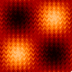
(a) $\rho=1/16$ and $3.5\times 10^{3}$

(b) $\rho=1$ and $\text{Pe}=1.4\times 10^{5}$

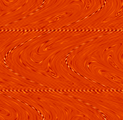
(c) $\rho=32$ and $\text{Pe}=1.4\times 10^{5}$

Figure 4: Snapshots of the scalar fields (left panels) and their normalized variance spectrum (right panel) for various values of $\rho$ and Pe. The dotted line shows Batchelor’s $k^{-1}$ power-law prediction for the spectrum. The vertical dash-dot line shows the location of the Batchelor wavenumber $k_{{}_{B}}=1/\ell_{{}_{B}}$. The vertical dash-dot-dot-dot line shows the location of the dissipation waver number, $k_{d}$. For figure 4(c), the dashed line in the variance spectrum (right panel) shows the $k^{+1}$ scaling that is related to the $\delta$-like structures shown in the left panel.

5.2 Spatial structures

It is interesting to relate the variation of the dissipation wavenumber with the different spatial structures of the scalar field that result from varying $\rho$. Figures 4(a-c) show three snapshots of $\theta(\bm{x},t)$ obtained for three different values of $\rho$, chosen for their clear representation of the different spatial structures that can be obtained. Also shown in the same figures are the time-averaged variance spectra, $\sigma^{2}_{k}$, defined in terms of $\hat{\theta}_{\bm{q}}(t)$, where $\theta(\bm{x},t)=\Sigma_{\bm{q}}\hat{\theta}_{\bm{q}}(t)e^{\bm{q}\cdot\bm{x}}$:

$$\sigma_{k}^{2}=\frac{1}{T_{2}-T_{1}}\int_{T_{1}}^{T_{2}}\sum_{k\leq|\bm{q}|<k+1}|\hat{\theta}_{\bm{q}}(t)|^{2}dt,$$ (44)

where $T_{1}$ is chosen to be sufficiently large for a steady state to have for long been established and $T_{2}-T_{1}\gg\tau$.

Figure 4(a) displays the case of $\rho=1/16$ and $\text{Pe}=3.5\times 10^{3}$. This set of values corresponds more closely to the homogenization Regime V (see also figure 2). The scalar field (left panel) is essentially a superposition of a large-scale component that is proportional to the source field and a small-scale component that is generated by the stirring velocity field. This superposition is clearly depicted in the spectrum of the variance (right panel) in which we observe that the majority of the scalar variance is concentrated on a single wavenumber which corresponds to the characteristic wavenumber of the source, $k_{s}\equiv 1/\ell_{s}$. Small-scale fluctuations are present for $k_{{}_{B}}<k<k_{u}$, where $k_{u}\equiv 1/\ell_{u}$ is the characteristic wavenumber of the velocity and $k_{{}_{B}}\equiv 1/\ell_{{}_{B}}$ is the Batchelor wavenumber beyond which the spectrum falls off exponentially. The spectrum associated with the small-scale fluctuations exhibits a power-law scaling with an exponent that is somewhat smaller than the Batchelor prediction of $-1$. The difference between $k_{d}$ and $k_{{}_{B}}$ arises because of the large concentration of scalar variance at small wavenumbers which shifts the value of $k_{d}$ to values smaller than $k_{{}_{B}}$. With decreasing $\rho$, the amplitude of the large-scale variance increases and so does the difference between $k_{d}$ and $k_{{}_{B}}$.

Figure 4(b) displays the case of $\rho=1$ and $\text{Pe}=1.4\times 10^{5}$ that most closely corresponds to Regime III. For this set of values, we observe the classical filamental structures that are obtained when stirring dominates. In this case, the field has no memory of the functional form of the source. For $k<k_{{}_{B}}$, the variance spectrum is characterized by a clean power-law that behaves in agreement with the Batchelor prediction.

Figure 4(c) displays the case of $\rho=32$ and $\text{Pe}=1.4\times 10^{5}$ which corresponds to the region of transition between Regime I and III (recall that for source (39) there is no Regime II). In this case, the flow is slowly varying with respect to the source. As a result, the scalar variance is, in the bulk of the domain, controlled by the process of sweeping between the sources and the sinks and thus its value is small. The only exception is a small number of isolated thin, boundary layers within which the scalar field is highly varying. These thin layers are formed in regions where the background flow is nearly stagnant so that the continual injection of scalar variance cannot be suppressed by the process of sweeping. For our particular flow (36) the regions of zero velocity are lines that, depending on time, are either vertical or horizontal. Thus, in each half of the period (horizontal/vertical) thin layers of alternating sign of $\theta$ are formed. These layers are similar to those obtained in Shaw et al. (2007) for a steady, sine flow. The (horizontal/vertical) thin layers that are formed in the first half of the period are then stretched in the second half at the same time as new (vertical/horizontal) thin layers are formed. The formation of these highly-varying, thin layers yields two power-law scalings for the variance spectrum: For small wavenumbers ($k<k_{s}$), the spectrum has a positive, power-law behaviour, given by $\sigma_{k}^{2}\sim k$. This behaviour can be deduced by noting that, for scales much larger than the source lengthscale, these structures are “$\delta$-like”. Conversely, for large wavenumbers - albeit smaller than the Batchelor wavenumber ($k_{s}<k<k_{{}_{B}}$), the Batchelor spectrum is recovered.

6 Conclusion

In this work we obtained a set of upper bounds for the dissipation wavenumber, $k_{d}$, of a continuously forced scalar field that is stirred by a spatially smooth velocity field. We focused on the dissipation wavenumber because it provides a measure for the enhancement of mixing due to the process of stirring. Unlike the freely decaying case in which stirring is the only mechanism for efficient mixing, in the forced case, transport can be as effective as stirring. This is clear from equation (2) in which it is easy to see that the scalar variance can be reduced either by increasing the dissipation wavenumber or by decreasing the correlation between the scalar and source fields.

Previous investigations have considered a number of mixing measures for which a set of bounds were derived (see Thiffeault et al. (2004); Plasting & Young (2006); Doering & Thiffeault (2006); Shaw et al. (2007)). However, these bounds do not always distinguish between the processes of stirring and transport. In particular, the bounds on the average variance of the scalar $\langle\theta^{2}\rangle$ and its gradient $\langle|\nabla\theta|^{2}\rangle$ do not explicitly depend on the velocity gradients. Thus, the effect of stirring is not captured. As a result, the bound for $k_{d}$ does not follow the scaling predicted in Batchelor (1959).

With the aid of an additional constraint, we here derived a new upper bound for $k_{d}$ which, within a range of values of Pe and $\rho$, is, up to a constant, equal to the inverse of the Batchelor lengthscale, $\ell_{{}_{B}}^{-1}$. The process of stirring is thus reflected in this bound. For large Péclet values, both the previous and the new bound become important, with the new bound significantly improving the previous bound for $\rho\gtrsim O(1)$. The scalings associated with these bounds suggest four different regimes for $k_{d}$. The use of homogenization theory implies a fifth regime. The most interesting, perhaps, behaviour occurs for $\rho\sim O(1)$. For these range of values of $\rho$, the scaling suggested by the upper bounds for $k_{d}$ transitions from a behaviour controlled by transport to a behaviour controlled by stirring. A summary of our results is provided in table 1.

Regime	$k^{2}_{d}$	range of validity	type
I	$\leqslant c_{2}/\ell_{s}^{2}$	$\rho\gg\text{Pe}$	diffusion-dominated regime
		$\rho\gg\text{Pe}^{\frac{1}{2}}$	(monochromatic source)
II	$\leqslant(c_{1}c_{2}U\ell_{s}/\kappa)^{\frac{1}{2}}/\ell_{s}^{2}$	$\text{Pe}^{\frac{1}{3}}\ll\rho\ll\text{Pe}$
		(absent)	(monochromatic source)
III	$\leqslant c_{3}/\ell_{{}_{B}}^{2}$	$O(1)\lesssim\rho\ll\text{Pe}^{\frac{1}{3}}$	Batchelor regime
		$O(1)\lesssim\rho\ll\text{Pe}^{\frac{1}{2}}$	(monochromatic source)
IV	$\leqslant c_{1}U/\kappa\ell_{s}$	$\text{min}\{1,\text{Pe}^{1-\alpha}\}\ll\rho\lesssim O(1)$
V	$\sim\rho^{2}\text{Pe}^{\alpha-1}/\ell_{{}_{B}}^{2}$	$\rho\ll\text{min}\{1,\text{Pe}^{1-\alpha}\}$	homogenization regime

Table 1: The four regimes deduced from bounds (13) and (22) and from homogenization theory. Also noted the case of a monochromatic source satisfying equation (23) (adapted from review by Thiffeault (2011)).

We tested the relevance of our theoretical predictions for the particular example of the “alternating sine flow” and a monochromatic source. We considered a large range of values for $\rho$, covering more than three orders of magnitude: from $\rho\ll 1$ (in which case homogenization theory becomes relevant) to $\rho\gg 1$ (in which case diffusion starts to dominate). The theoretical results were shown in figure 2 to give a qualitatively good description of the non-trivial dependence of $k_{d}$ on $\rho$. In particular, the numerical results were found to share a similar scaling behaviour with the diffusion-dominated Regime I, saturating it for large values of $\rho$, and the Batchelor Regime III, with the agreement for the latter being closer for larger values of Pe. The scaling of Regime IV did not appear in our numerical results. Instead, we found that for sufficiently small $\rho$, the numerical results match prediction (42) that corresponds to Regime V. Thus, for these values of $\rho$, homogenization theory provides a better estimate to the estimates derived from the bounds. Since the transition between Regimes IV and V depends on the value of the Strouhal number St (see equation (43) and figure 3), we anticipate that when this becomes sufficiently small, the range of validity of Regime IV will become sufficiently large for its scaling to be realized in the numerics.

The numerically obtained values were, in some cases, found to be more than one order of magnitude smaller than the values estimated by the bounds (the exception being Regime I which for $\rho\gg 1$ is saturated). An enhancement of the bounds can, in general, be made by finding the optimal ‘test field’ $\psi$ in constraint (10) (see Doering & Thiffeault (2006); Shaw et al. (2007); Plasting & Young (2006)). Such variational methods are expected to only improve the prefactor and not the scaling of bound (13) (and thus Regime IV). In fact Plasting & Young (2006) have shown that for the particular example of the “alternating sine flow” and monochromatic source, the choice $\psi=s$ is optimal and any improvement relies on knowledge of $\chi$ that is generally unknown. Conversely, the leading-order term in bound (22) is independent of the choice of the ‘test field’ and thus, with the current constraints, such methods are not likely to improve the bound in Regime III. It should be noted, however, that the biggest advantage of these upper bounds lies in predicting (or, to be more exact, restricting) the scaling behaviour of the dissipation wavenumber and how this is controlled by the parameters of the system. In that respect, the present investigation has proven to be very fruitful.

We now discuss the relation of our results with a particular set of mixing measures, the so-called mixing efficiencies, $E_{p}$. These were defined in Doering & Thiffeault (2006) and Shaw et al. (2007) in terms of $\langle|\nabla^{p}\theta|^{2}\rangle$, for $p\in\mathbb{Z}$, and the same variances obtained for $\theta_{0}$ satisfying (1) in the absence of a flow (${\bf u}=0$):

$$E_{p}\equiv\sqrt{\frac{\langle|\nabla^{p}\theta_{0}|^{2}\rangle}{\langle|\nabla^{p}\theta|^{2}\rangle}}.$$ (45)

$E_{p}$ are commonly larger than unity. In the high-Péclet limit and for spatially smooth source fields, they were shown to satisfy $E_{p}\lesssim\text{Pe}/\rho$, for $p=-1,0,1$. Using $\theta_{0}=\frac{1}{\kappa}\nabla^{-2}s$ and equation (2) into the definition for $E_{0}$, we obtain that

$$E_{0}=c_{4}\frac{k_{d}^{2}\ell_{s}^{2}}{\xi_{\theta,s}},$$ (46)

where $c_{4}$ is a non-dimensional number defined as $c_{4}=\langle(\hat{\Delta}^{-1}s)^{2}\rangle^{1/2}/{S}$ (the hat symbol denotes differentiation with respect to $\hat{\bm{x}}=\bm{x}/\ell_{s}$). Similarly, using equation (6),

$$E_{1}=c_{5}\frac{k_{d}\ell_{s}}{\xi_{\theta,s}},$$ (47)

where $c_{5}$ is a non-dimensional number defined as $c_{5}=\langle(\hat{\nabla}^{-1}s)^{2}\rangle^{1/2}/{S}$. Thus, neither $E_{0}$ nor $E_{1}$ include separate information about $k_{d}$ or $\xi_{\theta,s}^{-1}$. Since we have no control over the value of $\xi_{\theta,s}$, we cannot directly compare the bounds for $k_{d}$ with those for $E_{0}$ or $E_{1}$. Instead, the two sets of bounds provide complementary information. We note that from equations (46) and (47), we expect that if the suppression of variance is solely due to the suppression of $\xi_{\theta,s}$ (the case of a uniform flow), the two efficiencies $E_{0}$ and $E_{1}$ should scale similarly with Pe. If however the suppression of the variance is due to an increase in $k_{d}$, $E_{0}$ and $E_{1}$ are expected to scale differently. A separate investigation of the behaviour of $k_{d}$ and $\xi_{\theta,s}$ will be useful to clarify the types of flow that suppress the scalar variance mainly due to transport and those that do so mainly due to stirring.

Throughout this paper we have been working under the assumption that the spatial gradients of the velocity and the source fields are finite. Still, it is worth speculating on the implications of our results for rough sources and flows. The case of rough sources was considered in Doering & Thiffeault (2006); Shaw et al. (2007) for the mixing efficiencies (45). In this case, the roughness exponent of the source becomes crucial. For our bound (22), the source roughness will change the balance of the three terms inside the square root in equation (22), giving rise to different scalings for the dissipation lengthscale. A detailed examination would need to be performed to detemine the scaling behaviour in this case.

The case of rough velocity fields is also very important because of its relevance to turbulent flows. Although in this case bound (22) can not be defined, it is still worth examining the implications of our results using simple scaling arguments at the cost of losing some of the mathematical rigor. In three-dimensional turbulent flows, the most energetic scales, $L_{f}$, are large and control the transport between the sources and the sinks. Conversely, the smallest eddies have the largest shearing rate and control the stirring. A transition in the behaviour of $k_{d}$ is thus expected when bound (13) (that is still valid for rough velocity fields) intersects the Batchelor scaling, $k_{d}\sim\ell_{{}_{B}}^{-1}$. In terms of the Reynolds number, $\mathrm{Re}\equiv UL_{f}/\nu$ (where $\nu$ is the kinematic viscosity), the Batchelor scale reads,

$$\ell_{{}_{B}}^{2}\sim\frac{\kappa L_{f}}{U}\mathrm{Re}^{-\frac{1}{2}},$$ (48)

where we assume that $\text{Pe}\gg\mathrm{Re}$. Comparing (48) with bound (13), we obtain that a transition occurs when $\ell_{s}\sim\ell_{s}^{\ast}\equiv L_{f}\mathrm{Re}^{-\frac{1}{2}}$. For $\ell_{s}\lesssim\ell_{s}^{\ast}$, the scaling $k_{d}^{2}\sim\ell_{{}_{B}}^{-2}$ holds while for $\ell_{s}\gtrsim\ell_{s}^{\ast}$, bound (13) becomes smaller than $\ell_{{}_{B}}^{-1}$ and the scaling induced from (29) is expected. This prediction, however, should still be verified by numerical simulations.

We plan to address a number of the above mentioned issues in our future work.