Controllable Goos-Hänchen shifts and spin beam splitter for ballistic electrons in a parabolic quantum well under a uniform magnetic field

Abstract

The quantum Goos-Hänchen shift for ballistic electrons is investigated in a parabolic potential well under a uniform vertical magnetic field. It is found that the Goos-Hänchen shift can be negative as well as positive, and becomes zero at transmission resonances. The beam shift depends not only on the incident energy and incidence angle, but also on the magnetic field and Landau quantum number. Based on these phenomena, we propose an alternative way to realize the spin beam splitter in the proposed spintronic device, which can completely separate spin-up and spin-down electron beams by negative and positive Goos-Hänchen shifts.

I Introduction

The longitudinal Goos-Hänchen shift is well known for a light beam totally reflected from an interface between two dielectric media Lotsch . This phenomenon, suggested by Sir Isaac Newton, was observed firstly in microwave experiment by Goos and Hänchen Goos and theoretically explained by Artmann in term of stationary phase method Artmann . Up till now, the investigations of the Goos-Hänchen shift have been extended to different areas of physics Lotsch , such as quantum mechanics Renard ; Carter , acoustics Briers , neutron physics Ignatovich ; Haan , spintronics Chen-PRB , atom optics Zhang-WP , and graphene Zhao ; Beenakker-PRL ; Sharma , based on the particle-wave duality in quantum mechanics.

Historically, the quantum Goos-Hänchen shifts and relevant transverse Imbert-Fedorov shifts have been once studied for relativistic Dirac electrons in 1970s Miller ; Fradkin . With the development of the semiconductor technology, the Goos-Hänchen shift for ballistic electrons in two-dimensional electron gas (2DEG) system becomes one of the important subjects on the ballistic electron wave optics Wilson-G-G ; Sinitsyn ; XChen-PLA ; XChen-JAP . It was found that the lateral shifts of ballistic electrons transmitted through a semiconductor quantum barrier or well can be enhanced by transmission resonances, and become negative as well as positive XChen-JAP . The interesting Goos-Hänchen shift, depending on the spin polarization, could also provide an alternative way to realize the spin filter and spin beam splitter in spintronics Chen-PRB , in the same way as other optical-like phenomena including double refraction Ramaglia and negative refraction Zhang in spintronics optics Khodas .

In this paper, we will investigate the Goos-Hänchen shifts for ballistic electrons in a parabolic quantum well under a uniform magnetic field, in which the high spin polarization and electron transmission probability can be achieved Wan . It is shown that the lateral shift can be negative as well as positive. As a matter of fact, the Goos-Hänchen shift discussed here is different from that in the magnetic-electric nanostructure Chen-PRB , where the $\delta$ magnetic field is considered. In such quantum well, the uniform magnetic field bends the trajectory of electron continuously, so that electrons exhibit cyclotron motion. Then this implies that the behavior of electrons in such system has no direct analogy with linear propagation of light Sharma . Meanwhile, it is also suggested that Landau quantum number will have great effect on the Goos-Hänchen shift. We consider the Goos-Hänchen shift for ballistic electrons in a parabolic quantum well under a uniform magnetic field and its dependence on the magnetic field and Landau energy level, which to our knowledge, has not been investigated so far. More importantly, the Goos-Hänchen shift for ballistic electrons depends on the spin polarization by Zeeman interaction, which is similar to that for neutrons Haan . The realization of the negative and positive Goos-Hänchen shifts corresponding to spin-up and spin-down polarized electrons may have future applications in the proposed spintronic devices, such as spin filter and spin beam splitter.

II Theoretical model

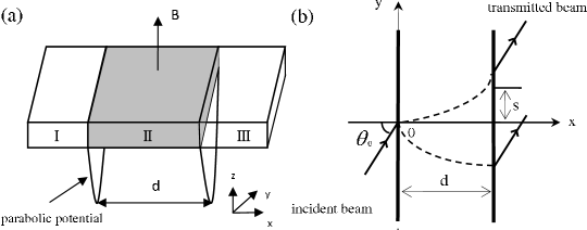
Figure 1: (a) Schematic diagram for 2DEG with the parabolic quantum well under a uniform magnetic field. (b) Negative and positive Goos-Hänchen shifts of ballistic electrons are presented in this configuration.

We consider a 2DEG structure, with a confining potential in the central region, as shown in Fig. 1 (a). The confinement potential is assumed to be parabolic in the transverse $y$ direction and the electron transports in the 2DEG occur in the plane of $x$-$y$. A uniform magnetic $B$ field is applied along the perpendicular $z$ direction and limited to within the parabolic confinement region. In practice, such a $B$-field configuration can be achieved by means of a ferromagnetic gate stripe on top of the 2EDG heterostructure Wan . The Hamiltonian within the parabolic quantum well is then given by

$$H=(1/2m)(\textbf{p}-\textbf{A})^{2}+H_{conf}+H_{z}$$ (1)

where $m$ is the effective mass of the electron and $\mathbf{p}$ is the momentum of the electron. The Landau gauge is chosen for the magnetic vector potential, i.e., $\textbf{A}=(By,0,0)$, where $B$ is the magnetic field strength. The parabolic confinement energy can be expressed as $H_{conf}=\frac{1}{2}m\omega_{0}^{2}y^{2}$, while the Zeeman interaction term is given by $H_{z}=\frac{1}{2}\mu_{B}g\sigma B$, so $\mu_{B}$ is the Bohr magneton, $g$ is Landé factor and $\sigma=\pm 1$ denotes the spin orientation parallel or antiparallel to the reference $z$ axis. In this system, the wave functions of plane wave for electrons in three regions can be expressed as

$$\Psi_{I}(x,y) = (e^{ik_{x}x}+Ae^{-ik_{x}x})e^{ik_{y}y},~{}~{}~{}~{}~{}~{}~{}~{}x<0$$ (2)

$$\Psi_{II}(x,y) = (Be^{ik^{\prime}_{x}x}+Ce^{-ik^{\prime}_{x}x})\psi_{2}(y),~{}0<x<d$$ (3)

$$\Psi_{III}(x,y) = De^{ik_{x}(x-d)}e^{ik_{y}y},~{}~{}~{}~{}~{}~{}~{}~{}~{}~{}~{}~{}~{}~{}~{}~{}x>d$$ (4)

where $k_{x}=\sqrt{2mE/\hbar^{2}-k_{y}^{2}}$ is the traveling wave vector in 2DEG. The Schrödinger equation in the parabolic potential region can be written in the form of a harmonic oscillator centered at $\widetilde{Y}$ with angular frequency $\widetilde{\omega}_{c}$,

$$\left[\frac{m\widetilde{\omega}_{c}^{2}}{2}(y-\widetilde{Y})^{2}+\frac{m\omega_{0}^{2}\omega_{c}^{2}}{2\widetilde{\omega}_{c}^{2}}Y^{2}+\frac{\mu_{B}g\sigma}{2}B-\frac{\hbar^{2}}{2m}\frac{d^{2}}{dy^{2}}\right]\Psi_{II}$$

$$~{}~{}~{}~{}~{}~{}~{}~{}~{}~{}~{}~{}~{}~{}~{}~{}~{}~{}~{}~{}~{}~{}~{}~{}~{}~{}~{}~{}~{}~{}~{}~{}~{}~{}~{}~{}~{}~{}~{}~{}~{}~{}~{}~{}~{}~{}~{}~{}~{}~{}~{}~{}~{}=E\Psi_{II}.$$ (5)

with $\widetilde{Y}=(\omega_{c}/\widetilde{\omega}_{c})^{2}Y$, $\widetilde{\omega}_{c}^{2}=\omega_{0}^{2}+\omega_{c}^{2}$, $\omega_{c}=Be/m$, $Y=\hbar k^{\prime}_{x}/eB$, $\omega_{c}$ is the cyclotron frequency. So the solution is given by a linear combination of Hermite polynomials as follows:

$$\psi_{2}(y)=\left(\frac{1}{2^{n}n!\gamma\sqrt{\pi}}\right)^{1/2}e^{-[(y-\widetilde{Y})^{2}/2\gamma^{2}]}H_{n}\left(\frac{y-\widetilde{Y}}{\gamma}\right),$$ (6)

where $\gamma^{2}=\hbar/\sqrt{e^{2}B^{2}+m^{2}\omega^{2}_{0}}$. The corresponding eigenenergy is

$$E_{n}=(n+\frac{1}{2})\hbar\widetilde{\omega}_{c}+\frac{m\omega_{0}^{2}\omega_{c}^{2}}{2\widetilde{\omega}_{c}^{2}}Y^{2}+\frac{1}{2}\mu_{B}g\sigma B.$$ (7)

The eigenstates of the system form a set of Landau-like states with energy splitting proportional to $B$. Within the central potential region, the longitudinal wave vector $k^{\prime}_{x}$ is given by

$$k^{\prime}_{x}=\sqrt{\frac{2m\widetilde{\omega}_{c}^{2}[E_{n}-(n+\frac{1}{2})\hbar\widetilde{\omega}_{c}-\frac{1}{2}\mu_{B}g\sigma B]}{\hbar^{2}\omega_{0}^{2}}},$$ (8)

which is spin-dependent due to Zeeman interaction. Interestingly, when the only plane wave is considered, the spatial location of the eigenstates inside the region of potential well is around $Y=\hbar k^{\prime}_{x}/eB$, which can be rewritten by

$$Y=\nu(n,k^{\prime}_{x})\frac{\omega_{0}^{2}+\omega_{c}^{2}}{\omega_{c}\omega_{0}^{2}},$$ (9)

with the velocity

$$\nu(n,k^{\prime}_{x})=\frac{1}{\hbar}\frac{\partial E_{n}}{\partial k^{\prime}_{x}}=\frac{\omega_{0}^{2}}{\widetilde{\omega}_{c}^{2}}\frac{\hbar k^{\prime}_{x}}{m}.$$ (10)

The transverse location for each plane wave eigenstate is proportional to the velocity and magnetic field. From the classical viewpoint, the spatial shift can be reasonably explained by Lorentz force Datta . As a consequence, the transverse shifts for the forward and backward propagating states inside the central region are positive and negative, since Lorentz force is opposite for electrons moving in the opposite direction. However, the lateral shift predicted by Goos-Hänchen effects will be totally different. In what follows, we will discuss the spin-dependent Goos-Hänchen shift of electron beam, instead of plane wave, in such a configuration.

III Goos-Hänchen shifts and spin beam splitter

III.1 Stationary phase method

When the finite-sized incident electron beam is considered, the wave function of incident beam can be assumed to be

$$\Psi_{in}(x,y)=\frac{1}{\sqrt{2\pi}}\int A(k_{y}-k_{y0})e^{i(k_{x}x+k_{y}y)}dk_{y},$$ (11)

with the angular spectrum distribution $A(k_{y}-k_{y0})$ around the central wave vector $k_{y0}$, then the transmitted beam can be expressed by

$$\Psi_{tr}(x,y)=\frac{1}{\sqrt{2\pi}}\int DA(k_{y}-k_{y0})e^{i[k_{x}(x-d)+k_{y}y]}dk_{y},$$ (12)

where the transmission coefficient $D=\exp{(i\phi)/g}$ is determined by the boundary conditions at $x=0$ and $x=d$ with

$$g\exp{(i\phi)=\cos{(k^{\prime}_{x}d)}+i\left(\frac{k^{2}_{x}+k^{{}^{\prime}2}_{x}}{2k_{x}k^{\prime}_{x}}\right)\sin{(k^{\prime}_{x}d})},$$ (13)

which leads to the phase shift $\phi$ in term of

$$\tan\phi=\frac{k_{x}^{2}+k^{{}^{\prime}2}_{x}}{2k_{x}k^{\prime}_{x}}\tan(k_{x}^{{}^{\prime}}d).$$ (14)

To find the position where $\Psi_{tr}(x,y)$ is maximum, that is, the lateral shift of transmitted beam, we look for the place where the phase of transmitted beam $\Phi=k_{x}(x-d)+k_{y}y+\phi$, has an extremum when differentiated with respect to $k_{y}$, ie, $\partial\Phi/\partial k_{y}=0$ Bohm . So according to the stationary phase approximation, the Goos-Hänchen shift for ballistic electrons at $x=d$ is defined as Chen-PRB

$$s=-\frac{d\phi}{dk_{y0}}.$$ (15)

It is noted that the subscript $0$ denotes the value at $k_{y}=k_{y0}$, namely $\theta=\theta_{0}$. Thus, the Goos-Hänchen shift, as described in Fig. 1 (b), can be obtained by

$$s=\frac{d\tan\theta_{0}}{2g^{2}_{0}}\left(1-\frac{k^{{}^{\prime}2}_{x0}}{k_{x0}^{2}}\right)\frac{\sin{(2k^{\prime}_{x0}d)}}{2k^{\prime}_{x0}d},$$ (16)

where $\theta_{0}$ is the incidence angle and $\tan\theta_{0}=k_{y0}/k_{x0}$. Obviously, it is clearly seen from Eq. (16) that the Goos-Hänchen shifts are negative as well as positive, depending on the $k^{{}^{\prime}2}_{x0}/k^{2}_{x0}$ and $\sin{(2k^{\prime}_{x0}d)}$.

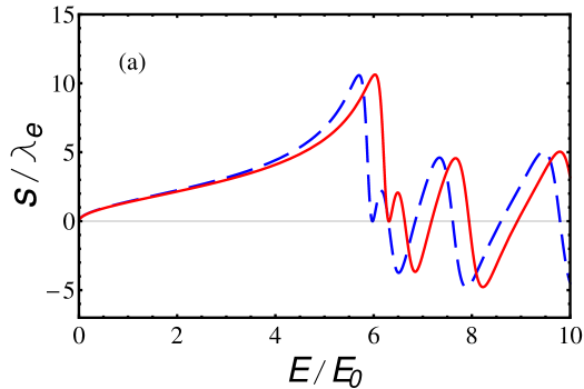
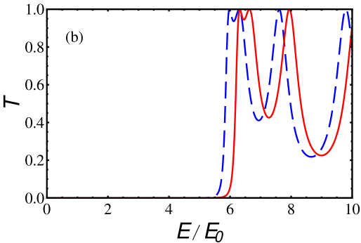
Figure 2: (Color online) Dependence of Goos-Hänchen shift (a) and transmission probability (b) on the incident energy $E/E_{0}$, where $\theta_{0}=70^{\circ}$ and the other physical parameters are respectively $m=0.013m_{e}$, $g=51$, $d=50$ nm, $B=0.5$ T and $n=5$. Solid (red) and dashed (blue) lines correspond to spin-up and spin-down polarized electrons.

In the propagating case, when the transmission resonances $k^{\prime}_{x0}d=m\pi~{}(m=1,2,3...)$ or anti-resonances $k^{\prime}_{x0}d=(m+1/2)\pi~{}(m=1,2,3...)$ occur, the Goos-Hänchen shift is zero, which means the positions in the $y$ direction are the same for both incident and transmitted electrons. As a matter of fact, when measured with reference to the geometrical prediction from electron optics, the “zero” lateral shifts will become essentially negative values. Whereas, when the incident energy is less than the critical energy,

$$E<E_{c}=(n+\frac{1}{2})\hbar\widetilde{w}_{c}+\frac{1}{2}\mu_{B}g\sigma B,$$ (17)

$k^{\prime}_{x0}$ becomes imaginary, thereby $k^{{}^{\prime}2}_{x0}/k^{2}_{x0}<0$. Substituting $k^{\prime}_{x0}=i\kappa_{0}$ into Eq. (16), we end up with the following expression:

$$s=\frac{d\tan\theta_{0}}{2g^{\prime 2}_{0}}\left(1+\frac{\kappa^{2}_{0}}{k_{x0}^{2}}\right)\frac{\sinh{(2\kappa_{0}d)}}{2\kappa_{0}d},$$ (18)

with

$$g^{{}^{\prime}2}_{0}=\cosh^{2}{(\kappa_{0}d)}+\left(\frac{k^{2}_{x}-\kappa^{2}_{0}}{2k_{x}\kappa_{0}}\right)^{2}\sinh^{2}{(\kappa_{0}d}).$$ (19)

In the evanescent case, the Goos-Hänchen shifts are always positive, which seems similar to the Goos-Hänchen shifts in a single semiconductor barrier XChen-PLA . In the opaque limit, $\kappa_{0}d\gg 1$, the lateral shift saturates to

$$s=\frac{2\kappa_{0}\tan\theta_{0}}{k_{x0}^{2}+\kappa^{2}_{0}}\simeq\frac{2\tan\theta_{0}}{\kappa_{0}},$$ (20)

which is independent of the width $d$ of potential well. In the following discussions, we will study the Goos-Hänchen shifts for different polarized electrons and their modulation by the magnetic field.

First of all, an example of the Goos-Hänchen shifts (in the units of $\lambda_{e}=2\pi\hbar/\sqrt{2m_{e}E}$) for ballistic electrons as function of incident energy $E/E_{0}$ in the quantum well under the uniform vertical magnetic field is displayed in Fig. 2 (a), where the quantum well is made from InSb semiconductor, the physical parameters are respectively $m=0.013m_{e}$, $m_{e}$ is the bare electron mass, $g=51$, the length of potential well $d=50$ nm, the parabolic well of depth, $\hbar\omega_{0}=2$ meV, the applied magnetic field $B=0.5$ T, $n=5$, and $E_{0}=\hbar\omega_{c}=4.45$ meV. It is clearly seen from the condition (17) that the critical energies are different for spin-up and spin-down polarized electrons, which correspond to $E^{+}_{c}=26.11$ meV and $E^{-}_{c}=27.58$ meV, respectively, for the parameters used here. As shown in Fig. 2 (a), the behavior of Goos-Hänchen shifts coincides with the theoretical analysis mentioned above, that is to say, the Goos-Hänchen shifts are always positive when the incident energy is less than the critical energy $E_{c}$, while the lateral shifts become negative as well as positive periodically related to the transmission resonances. In addition, Fig. 2 (b) also shows the dependence of transmission probability $T=|D|^{2}$ on the incident energy. This quantity can be connected with the measurable ballistic conductance $G$, according to the well-known Landauer-Büttiker formula at zero or non-zero temperature Datta ; Buttiker .

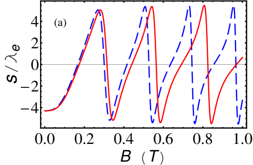
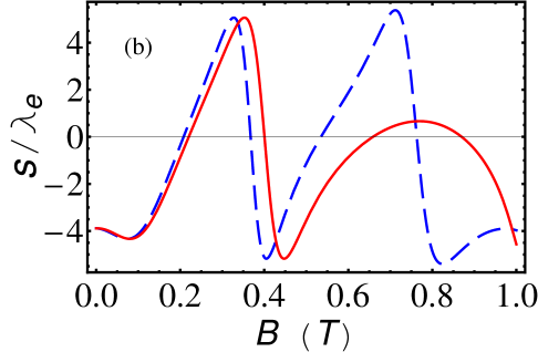
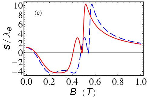
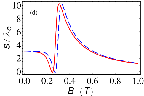
Figure 3: (Color online) Dependence of Goos-Hänchen shift on the strength of magnetic field $B$ with different Landau quantum number $n=0$ (a), $n=1$ (b), $n=3$ (c), $n=5$ (d), where $\theta_{0}=70^{\circ}$, $E=17.81$ meV, and the other physical parameters are the same as those in Fig. 2. Solid (red) and dashed (blue) lines correspond to spin-up and spin-down polarized electrons.

More interestingly, the spin-up and spin-down polarized electron beams can be separated by spatial shifts, due to their energy dispersion relation depending on the polarization. Based on the properties of Goos-Hänchen shifts, the simplest way to realize the energy filter by the Goos-Hänchen shifts is as follow. We can choose the incident energy within the range of $E^{+}_{c}<E<E^{-}_{c}$. This suggests that the spin-down polarized electrons for $E>E^{-}_{c}$ can traverse through the structure in the propagating mode with high transmission probability, while the spin-up polarized electrons for $E<E^{+}_{c}$ tunnel through it in the evanescent mode with very low transmission probability, as described in Fig. 2 (b). So this provides an alternative way to design a spin spatial filter with energy width $\Delta E=\mu_{B}gB=1.46$ meV for the parameters in Fig. 2.

Next, we will discuss the influence of magnetic field and Landau energy level on the Goos-Hänchen shifts in such semiconductor device. Figure 3 illustrates the dependence of Goos-Hänchen shifts on the strength of magnetic field $B$ with different Landau quantum number $n$, where $n=0$ (a), $n=1$ (b), $n=3$ (c), $n=5$ (d), $\theta_{0}=70^{\circ}$, $E=17.81$ meV, and the other physical parameters are the same as those in Fig. 2. Solid (red) and dashed (blue) lines correspond to spin-up and spin-down polarized electrons. Basically, the behavior of Goos-Hänchen shifts is different from that of transverse shifts for the plane wave, as described in Sec. II. According to the definition of critical energy $E_{c}$, under the low strength of magnetic field, the incident energy will be larger than the critical energy, thus the electron can propagate though the quantum well with negative and positive Goos-Hänchen shifts, which can be adjusted by the conditions for transmission resonances with changing magnetic fields. In other word, in the propagating case, the Goos-Hänchen shifts can be changed from negative to positive by controlling the strength of magnetic field, vice versa. However, the Goos-Hänchen shifts finally become positive with increasing the strength of magnetic field, due to the fact that the critical energy becomes larger than the incident energy with enough large magnetic field $B_{c}$, and the propagation of electrons is actually evanescent in this case. To understand the dependence of shifts on the magnetic field better, we have to calculate the critical magnetic field $B_{c}$ from Eq. (17) by solving the following equation, $(n+1/2)\hbar e^{2}B^{2}_{c}/m^{2}+\mu_{B}g\sigma B_{c}/2+(n+1/2)\hbar\omega^{2}_{0}-E=0$, for the fixed incident energy $E$. For example, the critical magnetic fields for spin-up and spin-down polarized electrons can be numerically obtained as follows: $B^{+}_{c}=1.02$ T and $B^{-}_{c}=1.48$ T for $n=1$, $B^{+}_{c}=0.49$ T and $B^{-}_{c}=0.55$ T for $n=3$, $B^{+}_{c}=0.28$ T and $B^{-}_{c}=0.30$ T for $n=5$. So these results can be applicable to explain the most striking effect around the critical magnetic field $B_{c}$ in Fig. 3 (b)-(d), while the similar behavior is not shown in Fig. 3 (a), because the critical magnetic fields, $B^{+}_{c}=3.00$ T and $B^{-}_{c}=5.98$ T for $n=0$, are too large, we just show the range of magnetic field from $0$ to $1$ T due to the physical restriction to applied magnetic field in the laboratory. In addition, another observation from Fig. 3 is that, with increasing Landau quantum number $n$, the curves of Goos-Hänchen shifts move leftwards. That is to say, for the given incident energy, Landau energy level leads to the fact that the resonant peak or the critical strength of magnetic field $B_{c}$ shifts towards the low magnetic field strength region as increasing Landau quantum number $n$. Compared to the previous results in the magnetic-electric nanostructure Chen-PRB , the magnetic field and Landau quantum number provide more freedom to control the quantum Goos-Hänchen shift for ballistic electrons, which is useful to its application in the semiconductor devices.

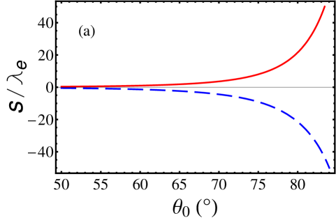
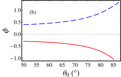
Figure 4: (Color online) Spin-dependent Goos-Hänchen shifts (a) and corresponding phase shifts (b) as the function of incidence angle, where $E/E_{0}=7.8$ and the other physical parameters are the same as those in Fig. 2. Solid (red) and dashed (blue) lines represent spin-up and spin-down polarized electrons, respectively.

Now, we will discuss the spin beam splitting by the spin-dependent Goos-Hänchen shifts at various incidence angles. In general, the Goos-Hänchen shifts can also be modulated by the incidence angles, due to the energy dispersion (8). In Fig. 4 (a), we would like to emphasize that the spin-up and spin-down polarized electrons can be spatially separated by the spin-dependent Goos-Hänchen shifts at large incidence angles, for example $\theta_{0}=80^{\circ}$, where incident energy $E/E_{0}=7.8$, and the other physical parameters are the same as those in Fig. 2. To confirm this intriguing result, the phase shifts of transmitted electrons have also been investigated in Fig. 4 (b). In detail, the negative slope of the phase shift with respect to the incidence angle will result in the positive Goos-Hänchen shift, whereas the positive one will lead to the negative Goos-Hänchen shift, which are in agreement with theoretical predictions by stationary phase method. Thus, the Goos-Hänchen shifts can be explained by the reshaping process of the transmitted beam, since each plane wave component undergoes the different phase shift due to the multiple reflections inside the quantum well XChen-PLA . The negative and positive beam shifts are usually considered as the consequence of constructive and destructive interferences between the plane wave components of electron beam.

III.2 Numerical simulation

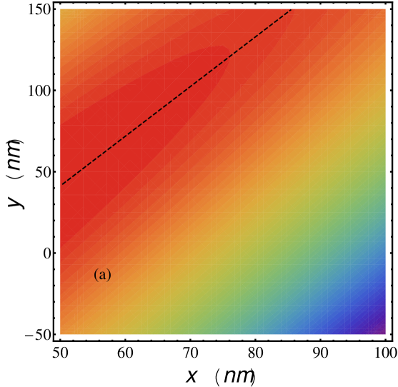
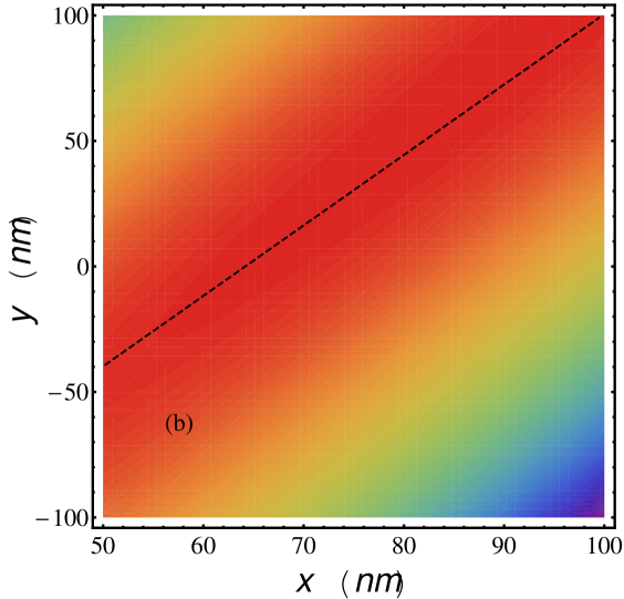
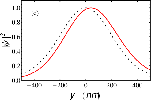
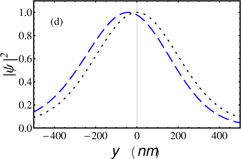
Figure 5: (Color online) Distribution of the transmitted Gaussian-shaped beam for spin-up (a) and spin-down (b) polarized electrons, where $\theta_{0}=80^{\circ}$, beam width is $w=5\lambda_{e}$, and the other physical parameters are the same as those in Fig. 2. Dashed lines represent the loci of maximum values for the eye. Profiles of the normalized incident and transmitted beams for spin-up (c) and spin-down (d) polarized electrons are also compared at $x=d$, where solid (red) and dashed (blue) lines represent the transmitted beams, and dotted (black) line represents the incident beam as reference.

In this section, we further process to make the numerical simulations of the incident Gaussian-shaped beam, $\Psi_{in}(x=0,y)=\exp(-y^{2}/2w^{2}_{y}+ik_{y0}y)$, where $w_{y}=w\sec\theta_{0}$, $w$ is the width of beam. According to Fourier integral, using Eqs. (11) and (12), we can obtain the wave function of transmitted beam as follows,

$$\Psi_{tr}(x,y)=\frac{1}{\sqrt{2\pi}}\int_{-k}^{k}DA(k_{y}-k_{y0})e^{i[k_{x}(x-d)+k_{y}y)]}dk_{y},$$ (21)

where $A(k_{y}-k_{y0})=w_{y}\exp[-(w^{2}_{y}/2)(k_{y}-k_{y0})^{2}]$. For a well-collimated the range of above integral can be ideally extended from $-\infty$ to $\infty$. Figs. 5 (a) and (b) illustrate the distribution of transmitted beam, $|\Psi_{tr}(x,y)|^{2}$, for spin-up and spin-down polarized electrons, where $\theta_{0}=80^{\circ}$, the beam width is $w=5\lambda_{e}$, and the other physical parameters are the same as those in Fig. 2. As demonstrated in Fig. 5 (a) and (b), dashed lines represent the loci of the maximum values for distribution of the transmitted beams for the eye. Evidently, the comparison between the normalized incident and transmitted beams at $x=d$ in Fig. 5 (c) and (d) show that the positive and negative lateral shifts correspond to the different spin polarization. To find the numerical value of beam shifts, we can find the position $y$ corresponds to the maximum value of $|\Psi_{tr}(x,y)|^{2}$. For the given parameters in Fig. 5, $y^{+}=40.80$ nm and $y^{-}=-43.21$ nm can be achieved for spin-up and spin-down polarized electrons, which are large enough to sperate the different spin-polarized electrons beam spatially.

In Fig. 6, the numerical results further show the influence of beam width on Goos-Hänchen shifts and spin beam splitter, where the physical parameters are the same as those in Fig. 4 and the beam width is chosen to be $w=5\lambda_{e}$ and $w=10\lambda_{e}$ (corresponding to the beam divergence of $\delta\theta=4^{\circ}$ and $\delta\theta=2^{\circ}$). It is demonstrated that the wider the local waist of incident beam is, the closer to the theoretical results predicted by stationary phase method the numerical results are. It is worthwhile to point out that there is discrepancy between theoretical results predicted by stationary phase approximation and numerical results, resulting from the distortion of the transmitted electron beam XChen-PLA ; Chen-PRB , especially when the local beam waist is narrow, which implies large beam divergent $\delta\theta=\lambda_{e}/(\pi w)$. Actually, the stationary phase approximation is valid only for well-collimated electron beam XChen-PLA ; Chen-PRB . In detail, when the incidence angle is small enough, the Goos-Hänchen shifts predicted by stationary phase method are in agreement with the results given by numerical simulations. But when a large incidence angle is chosen, $\delta\theta\ll 90^{\circ}-\theta_{0}$ is not satisfied, so that the transmitted beam shape will undergo severe distortion. It is suggested that one cannot achieve an arbitrary large Goos-Hänchen shift in practice by increasing the incidence angle, taking into account the influence of finite beam width. In a word, the theoretical results of stationary phase method and numerical simulations show that the simultaneously large and opposite beam shifts for spin-up and spin-down polarized electrons allow this system to realize the spin beam splitter, which can completely separate spin-up and spin-down polarized electrons in such semiconductor quantum device.

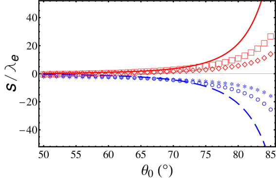
Figure 6: (Color online) Influence of beam width on the Goos-Hänchen shifts, where the physical parameters are the same as those in Fig. 4. Solid (red) and dashed (blue) lines represent the shifts for spin-up and spin-down polarized electrons, calculated by stationary phase method. Lines with markers “$\square$” (“$\circ$”) and “$\diamond$” (“$\ast$”) correspond to the numerical results for spin-up (spin-down) polarization with $w=10\lambda_{e}$ and $w=5\lambda_{e}$, respectively.

IV Discussion and Conclusion

We have investigated the Goos-Hänchen shift for ballistic electrons through a parabolic quantum well under a uniform magnetic field. Due to the effect of magnetic field, the Goos-Hänchen shift for ballistic electrons also becomes spin-dependent, which leads to the novel applications in designing the spin filter and spin beam splitter. It is found that the Goos-Hänchen shift can be modulated by the incident energy, magnetic field, Landau quantum number, and incidence angle. In addition, we would like to mention that the Goos-Hänchen shift is also sensitive to the device geometry, since the lateral shift depends periodically on the width $d$ of parabolic quantum well region. The spin-dependent Goos-Hänchen shift and spin beam splitter presented here can be discussed in GaAs/AlGaAs-based quantum well structure Wan , rather than InSb semiconductor with high $g$-factor.

Last but not least, the Goos-Hänchen shift and relevant transverse Imbert-Fedorov effect in such quantum well under the magnetic field may have close relation to spin Hall effect Sinitsyn ; Onoda ; Bliokh , which deserves further investigations. We hope all the results presented here will stimulate further theoretical and experimental researches on quantum Goos-Hänchen shifts for ballistic electrons in semiconductor Chen-PRB ; XChen-JAP and graphene Beenakker-PRL ; Wu and their applications in various quantum electronic devices.

References

- (1) H. K. V. Lotsch, Optik (Stuttgart) 32, 116 (1970); 32, 189 (1970); 32, 299 (1971); 32, 553 (1971).
- (2) F. Goos and H. Hänchen, Ann. Phys. 1, 333 (1947); 5, 251 (1949).
- (3) K. V. Artmann, Ann. Phys. (Leipzig) 2, 87 (1948).
- (4) R.-H. Renard, J. Opt. Soc. Am. 54, 1190 (1964).
- (5) J. L. Carter and H. Hora, J. Opt. Soc. Am. 61, 1640 (1971).
- (6) R. Briers, O. Leroy, and G. Shkerdinb, J. Acoust. Soc. Am. 108, 1624 (2000).
- (7) V. K. Ignatovich, Phys. Lett. A 322, 36 (2004).
- (8) Victor-O. deHaan, J. Plomp, Theo M. Rekveldt, W. H. Kraan, Ad A. van Well, R. M. Dalgliesh, and S. Langridge, Phys. Rev. Lett. 104, 010401 (2010).
- (9) X. Chen, C.-F. Li, and Y. Ban, Phys. Rev. B 77, 073307 (2008).
- (10) J.-H. Huang, Z.-L. Duan, H.-Y. Ling, and W.-P. Zhang, Phys. Rev. A 77, 063608 (2008).
- (11) L. Zhao and S. F. Yelin, Phys. Rev. B 81, 115441 (2010); arXiv:0804.2225v2.
- (12) C. W. J. Beenakker, R. A. Sepkhanov, A. R. Akhmerov, and J. Tworzydło, Phys. Rev. Lett. 102, 146804 (2009).
- (13) M. Sharma and S. Ghosh, J. Phys.: Condens. Matter 23, 055501 (2011).
- (14) S. C. Miller, Jr., and N. Ashby, Phys. Rev. Lett. 29, 740 (1972).
- (15) D. M. Fradkin and R. J. Kashuba, Phys. Rev. D 9, 2775 (1974); 10, 1137 (1974).
- (16) D. W. Wilson, E. N. Glytsis, and T. K. Gaylord, IEEE J. Quantum Electron. 29, 1364 (1993).
- (17) N. A. Sinitsyn, Q. Niu, J. Sinova, and K. Nomura, Phys. Rev. B 72, 045346 (2005).
- (18) X. Chen, C.-F. Li, and Y. Ban, Phys. Lett. A 354, 161 (2006).
- (19) X. Chen, Y. Ban, and C.-F. Li, J. Appl. Phys. 105, 093710 (2009).
- (20) V. M. Ramaglia, D. Bercioux, V. Cataudella, G. D. Filippis, and C. A. Perroni, J. Phys.: Condens. Matter. 16, 9143 (2004).
- (21) X.-D. Zhang, Appl. Phys. Lett. 88, 052114 (2006).
- (22) M. Khodas, A. Shekhter, and A. M. Finkel’stein, Phys. Rev. Lett. 92, 086602 (2004).
- (23) F. Wan, M. B. A. Jalil, S. G. Tan, and T. Fujita, J. Appl. Phys. 103, 07B731 (2008); Int. J. of Nanoscience 8, 71 (2009).
- (24) S. Datta, Electronic transport in mesoscopic system, Cambridege University Press, 1995.
- (25) D. Bohm, Quantum Theory, Prentice-Hall, New York, 1951, p. 259.
- (26) M. Büttiker, Phys. Rev. Lett. 57, 1761 (1986).
- (27) M. Onoda, S. Murakami, and N. Nagaosa, Phys. Rev. Lett. 93, 083901 (2004).
- (28) K. Yu. Bliokh and V. D. Freilikher, Phys. Rev. B 74, 174302 (2006).
- (29) Z.-H. Wu, F. Zhai, F. M. Peeters, H. Q. Xu, K. Chang, arXiv:1008.4858v3.