Impurity Effects in Highly Frustrated Diamond Lattice Antiferromagnets

Abstract

We consider the effects of local impurities in highly frustrated diamond lattice antiferromagnets, which exhibit large but non-extensive ground state degeneracies. Such models are appropriate to many A-site magnetic spinels. We argue very generally that sufficiently dilute impurities induce an ordered magnetic ground state, and provide a mechanism of degeneracy breaking. The states which are selected can be determined by a “swiss cheese model” analysis, which we demonstrate numerically for a particular impurity model in this case. Moreover, we present criteria for estimating the stability of the resulting ordered phase to a competing frozen (spin glass) one. The results may explain the contrasting finding of frozen and ordered ground states in CoAl₂O₄ and MnSc₂S₄, respectively.

I Introduction

A common feature of highly frustrated magnets is the existence of a large (classical) ground state degeneracy in model Hamiltonians.Moessner and Ramirez (2006) Although this degeneracy is accidental, in the sense that the multitude of ground states are generally not symmetry-related, it nevertheless yields striking physical consequences. For instance, over a broad temperature range the system resides in a “cooperative paramagnetic” or “classical spin liquid” regime, where the spins avoid long-range order but fluctuate predominantly within the ground state manifold. The ultimate fate of such highly frustrated spins at the lowest temperatures poses an interesting and experimentally important problem. Typically, at very low temperatures entropic or quantum fluctuations alone are sufficient to lift the degeneracy and produce an ordering transition via “order by disorder”.Villain et al. (1980); Henley (1989) However, additional weak effects which would otherwise be negligible in unfrustrated systems—such as small further-neighbor exchangeBergman et al. (2006, 2007), spin-lattice couplingYamashita and Ueda (2000); Bergman et al. (2006), and dipolar interactionsBramwell and Gingras (2001)—can also provide a degeneracy-lifting mechanism, which indeed often dominates over fluctuation effects.

In this paper we discuss degeneracy breaking by quenched random impurities. Generally even a non-magnetic defect (i.e. one which does not break spin-rotational symmetry) such as a random bond, an interstitial spin, or a vacancy, will locally distinguish the various degenerate states of the pristine system. This brings up a number of issues. First, can impurities consequently lead to ordering, i.e. “order by quenched disorder”? Or, by virtue of their randomness, do they lead instead to a glassy disordered state? Do these impurities influence the spins in their vicinity independently from one another? Or are their effects rendered highly coordinated by the correlated nature of fluctuations in the cooperative paramagnetic regime?

The answers to these questions probably depend in detail upon the nature of the magnetic system under consideration, particularly the degree of frustration. Generally, with increasing frustration comes increasing ground state degeneracy. One often useful characterization scheme for frustration involves counting the distinct magnetic ordering wavevectors which are possible within the classical ground state manifold. In mildly frustrated magnets, such as the nearest-neighbor triangular antiferromagnet, this wavevector is unique. In the nearest-neighbor fcc antiferromagnet, the ordering wavevectors form continuous one-dimensional lines.Gvozdikova and Zhitomirsky (2005) The much more frustrated nearest-neighbor kagome and pyrochlore antiferromagnets, by contrast, have ordering wavevectors that fill all of reciprocal space.Chalker et al. (1992); Reimers et al. (1991)

In the latter kagome and pyrochlore cases, the degeneracy is local—i.e. the ground state entropy is extensive, and states within the ground state manifold are related by modifications of only a small number of spins. An impurity can then fix the spin configuration in its neighborhood, while constraining the spins outside of its vicinity very little.Shender et al. (1993) Since each random impurity fixes a spin configuration in its neighborhood, roughly independently of the others, one may expect as a result a globally random ground state, i.e. a spin glass. In fact, the $T>0$ dynamics of such defective pyrochlore and kagome systems is rather subtle, and the actual spin glass freezing temperature can sometimes be highly suppressed as a result.Shender et al. (1993) Nevertheless, spin glass behavior is very commonly observed in highly frustrated magnets,Ramirez (1994) even when the disorder is nominally very weak.

For the other classes of frustrated systems noted above, in which the ground state ordering wavevectors occupy a smaller subset of reciprocal space, the degeneracy is sub-extensive. An infinite number of spins must then be varied in order to transform one ground state to another. Thus, different impurities cannot independently determine their local environments. In this paper, we develop a formalism for dealing with their effects, focusing for concreteness on the most degenerate case (of which we are aware) of a sub-extensive degeneracy: frustrated diamond lattice antiferromagnets. In a $J_{1}-J_{2}$ model on the diamond lattice, the ordering wavevectors (for antiferromagnetic $J_{2}>|J_{1}|/8$) form a 2d surface within the 3d momentum space.Bergman et al. (2007) This example is of particular recent interest due to its relevance to the A-site magnetic spinel materials, with chemical formula AB₂X₄, in which magnetic A sites form a diamond sublattice with non-magnetic B and X atoms.Fritsch et al. (2004); Tristan et al. (2005); Krimmel et al. (2006) Because it represents an extreme case of sub-extensive degeneracy, we expect that the conclusions obtained for this case apply fairly generally to other less degenerate frustrated magnets.

Our conclusion is that, for this class of systems, despite the large ground state degeneracy, long-range magnetic order is stabilized—and indeed a specific ground state is selected—at sufficiently low impurity concentrations. Each impurity induces a small, finite region around it in which the spins are deformed from an ideal spiral pattern, like holes in “swiss cheese” (Emmentaler). The swiss cheese model allows a calculation of the global ground state wavevector, based on certain properties of an individual defect. We calculate this wavevector for the A-site spinel case, with a specific impurity model. We show how the same theoretical framework determines other physical properties such as the ordered moment observed in neutron scattering, and the transition temperature. The swiss cheese model also signals its own demise, in one of two ways. First, if the holes in the cheese strongly overlap, the assumption of their independence fails. Second, even when the holes do not overlap, if the underlying “stiffness” of the bulk spiral is too small, then the impurities may induce strong fluctuations. In either case, the long-range order is expected to give way to a disordered spin glass ground state. These two possibilities provide criteria, whereby the stability of the ordered spiral state can be quantitatively estimated. In the case of the A-site spinels, we suggest that this method consistently explains the contrasting glassy and ordered ground states found in CoAl₂O₄MacDougall et al. (2011); Tristan et al. (2005) and MnSc₂S₄Krimmel et al. (2006); Fritsch et al. (2004); Giri et al. (2005), respectively.

The remainder of the paper is organized as follows. We consider a single impurity in Sec. II. Using a non-linear sigma model, it is shown quite generally that, on long length scales, a single defect can generate only small deformations away from a uniform spiral ground state of the clean system. We then demonstrate via Monte Carlo simulations that the classical degeneracy is indeed lifted by the impurity, which favors specific wavevectors along the spiral surface, thereby providing a mechanism of “order by quenched disorder”. A single impurity is further characterized by a length scale $\xi$ (the size of the hole) outside of which the spins are well-described by a uniform spiral. In Sec. III, we extend this analysis to the case of multiple impurities. There, we discuss the interplay between impurity and entropic effects, and make quantitative, verifiable predictions for how $T_{c}$ varies with impurity concentration. We conclude in Sec. IV with a discussion of our results in the context of experiments and impurity effects in other models.

II Single impurity

In this section, we discuss the physics of a single impurity. First, we will consider the possibility that the impurity induces a slow variation of the spins extending over infinite distances. By analyzing the energy as a function of order parameter variations, we show that this is not the case. Instead, the deformation of the spins by each impurity is local, and decays to a uniform spiral as the distance from the defect increases. We then show that the impurity physics can be characterized by an impurity energy function, $E_{a}(\mathbf{q})$, which gives the difference between the ground state energies of the system with and without a single impurity of type $a$, under the constraint that far from the impurity the spins adopt a spiral configuration with wavevector $\mathbf{q}$. Employing extensive Monte Carlo simulations we calculate this function numerically for a specific impurity model. In order to check the validity of the swiss-cheese model, we characterize the local region of deformation around an impurity: we compute locally the $q$-vector from Monte Carlo realizations of spin configurations. We find that in our simulations, variations of $q$ are extremely local, and most changes happen within one unit cell.

II.1 General considerations

Consider an arbitrary local defect, for which the Hamiltonian of the system can only be modified in a finite vicinity of the impurity (involving only a finite number of spins). Also, for simplicity, we will assume the defect is “non-magnetic”, meaning it preserves the spin-rotational invariance of the Hamiltonian.

The energy of the system in the presence of the impurity then consists of a contribution in the region where the defect has modified the Hamiltonian, and a contribution from the remainder of the system. For any spin configuration, the former is finite and the latter contains a leading term proportional to $V$ and subdominant corrections. By choosing the spin configuration equal to that of one of the ground states in the absence of the defect, we can make the energy density $E/V=\epsilon_{0}$ in the large $V\rightarrow\infty$ limit equal to that of the pure system, and therefore the ground states in the presence of the impurity must also achieve this same energy density $\epsilon_{0}$. This implies that spins far from the impurity must locally resemble one of the ground states of the pure system.

II.1.1 Spiral order parameter

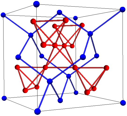
Figure 1: Cubic cell of an AB₂X₄ spinel. The sublattice of A sites (blue spheres) is a diamond lattice, while the sublattice of B sites (red spheres) is a pyrochlore lattice.

To make our discussion more concrete, we now specialize to the case of the frustrated diamond lattice antiferromagnet with first and second nearest neighbor interactions. The ground states of this system were determined in Ref. Bergman et al., 2007. For $J_{2}/|J_{1}|>1/8$, which is the parameter regime we focus on hereafter, they consist of coplanar spirals whose propagation wavevector ${\bf q}$ lies anywhere on a continuous “spiral surface” in reciprocal space. The configuration of the spiral is described by

$$\vec{S}({\bf r})={\rm Re}\left[\vec{d}\,e^{i{\bf q}\cdot{\bf r}+i\gamma({\bf q};{\bf r})}\right],$$ (1)

where the phase $\gamma({\bf q};{\bf r})=\pm\gamma({\bf q})$ when ${\bf r}$ is on the I or II diamond sublattice, respectively. (The parametrization is such that the I diamond sublattice contains the site at $(0,0,0)$ and the II sublattice that at $\frac{1}{8}(1,1,1)$). The vector $\vec{d}$ specifies the plane of the spiral in spin space and its phase. It takes the form

$${\vec{d}}=\hat{e}_{1}+i\hat{e}_{2},$$ (2)

where $\hat{e}_{1},\hat{e}_{2}$ are orthogonal unit vectors and $|\vec{d}|$ is fixed at $\sqrt{2}$. The spiral surface itself (i.e. the locus of allowed ${\bf q}$) deforms smoothly with $J_{2}/|J_{1}|$ (except at the isolated value of $J_{2}/|J_{1}|=1/4$ where it changes topology).

To specify a ground state, one must therefore specify both $\vec{d}$ and the wavevector ${\bf q}$, constrained to the spiral surface. One can then regard $(\vec{d},{\bf q})$ as the order parameter. Far from the impurity, the spin configuration must locally take the ground state form of Eq. (1), but we must consider the possibility that these parameters may vary slowly (relative to the largest micro-scale of the spiral, the wavelength $2\pi/|q|$) in space. We will now argue that such variations are insignificant: far from the impurity, the spiral wavevector and the $\vec{d}$ vector are uniform in the ground state (and indeed all finite energy states).

To do so, we consider the energy of a slowly-varying order parameter that is macroscopically non-uniform and show that it is divergent. Encoding the slow variations naïvely requires $5$ continuous real functions: three angles to specify $\vec{d}$, and two more to specify the position of ${\bf q}$ on the surface. However, the actual number of degrees of freedom is smaller due to an additional gauge symmetry: To see this we note that a change in the wavevector, ${\bf q}\rightarrow{\bf q}+\delta{\bf q}$ can be compensated by the shift ${\vec{d}}\rightarrow{\vec{d}}e^{-i\delta{\bf q}\cdot{\bf r}-i\delta\gamma}$ with no change to the spins (here $\delta\gamma=\gamma({\bf q+\delta q})-\gamma({\bf q})$). Therefore there is a “gauge” redundancy in these variables. We can “fix” the gauge in a variety of ways. A simple choice is to allow only for spatial variations in $d$ and not in ${\bf q}$, i.e. we write:

$$\vec{S}({\bf r})={\rm Re}\left[\vec{d}({\bf r})\,e^{i{\bf q}_{0}\cdot{\bf r}+i\gamma({\bf q};{\bf r})}\right],$$ (3)

where $\vec{d}({\bf r})$ is assumed to be slowly varying in space, and ${\bf q}_{0}$ is a constant “reference” wavevector. We emphasize that this still allows the physical wavevector to be different from ${\bf q}_{0}$. For instance, if $\vec{d}({\bf r})=\vec{d}_{0}e^{i\delta{\bf q}\cdot{\bf r}}$ with constant $\vec{d}_{0}$, the physical wavevector is ${\bf q}={\bf q}_{0}+\delta{\bf q}$. In general, we can define the physical wavevector as

$$q^{\mu}=q^{\mu}_{0}+\frac{1}{2}{\rm Im}\left[\vec{d}^{*}\cdot\partial_{\mu}\vec{d}\right].$$ (4)

Note that for Eq. (3) to correspond locally to a proper minimum energy spiral ground state, the first argument ${\bf q}$ of $\gamma$ must be the physical wavevector given by Eq. (4), not ${\bf q}_{0}$.

II.1.2 Energy of weakly deformed spirals

It is sufficient to consider just small spatial variations of $\vec{d}$, since we will find that these are already prohibitively costly at long distances. Let

$$\vec{d}({\bf r})=\vec{d}_{0}+\delta\vec{d}({\bf r}).$$ (5)

To preserve the unit vector constraint of the spins $\vec{S}^{2}=1$ in Eq. (3), a small $\delta\vec{d}({\bf r})$ must be of the form

$$\delta\vec{d}({\bf r})=i\phi({\bf r})\vec{d}_{0}+\psi({\bf r})\hat{e}_{3},$$ (6)

where $\phi$ and $\psi$ are arbitrary small real and complex fields, respectively, and

$$\hat{e}_{3}=\hat{e}_{1}\times\hat{e}_{2}=-\frac{1}{2}{\rm Im}\left[\vec{d}\times\vec{d}^{*}\right].$$ (7)

$\phi$ describes the rotation of the vector $\vec{d}$ within the spiral plane (spanned by $\hat{e}_{1},\hat{e}_{2}$), and includes simple variations in the physical wavevector, while $\psi$ describes variations outside the spiral plane. To this linearized order, we have simply ${\bf q}={\bf q}_{0}+{\boldsymbol{\nabla}}\phi$.

Now consider the energy density as a function of $\phi,\psi$ and their gradients. First, the energy must be unchanged for constant values of these functions, since these correspond to global $O(3)$ spin rotations. The first non-trivial terms in a Taylor expansion can arise at quadratic order in these fields, and from the above reasoning, must include only spatial gradients so that they vanish for constant configurations. Finally, this quadratic form must be positive semi-definite, because the un-deformed configuration obtains the minimal energy.

An additional constraint is given by frustration: the energy must also be unchanged for deformations corresponding to changes of the wavevector within the spiral surface. Such a deformation is of the form $\phi({\bf r})=\delta{\bf q}\cdot{\bf r}$, where $\delta{\bf q}$ is an arbitrary (small) vector in the plane tangent to the spiral surface at ${\bf q}_{0}$. This constraint is highly restrictive. Consider the structure of allowed quadratic terms in $\phi$ with two gradients:

$${\mathcal{E}}_{\phi}=\frac{1}{2}c_{\mu\nu}\partial_{\mu}\phi\partial_{\nu}\phi,$$ (8)

where a sum over $\mu,\nu$ is implied, and $c_{\mu\nu}$ is an arbitrary real symmetric matrix. This energy density should vanish for a deformation corresponding to a constant spiral with a wavevector shifted slightly within the spiral surface, which implies

$$c_{\mu\nu}\delta q^{\mu}\delta q^{\nu}=0,$$ (9)

for $\delta{\bf q}$ in the tangent plane. Eq. (9) reduces $c_{\mu\nu}$ to a single undetermined coefficient $c$, such that $c_{\mu\nu}=c\hat{n}_{\mu}\hat{n}_{\nu}$, where $\hat{\bf n}$ is the unit normal vector to the spiral surface. The energy cost to deform $\phi$ in the directions parallel to the spiral surface is thus higher order in derivatives. Along the same lines one may deduce the most general allowed energy density quadratic in the $\phi,\psi$ fields with the minimal number of gradients to ensure stability:

$${\mathcal{E}} = \frac{c}{2}(\nabla_{\perp}\phi)^{2}+c^{\prime}\nabla_{\perp}\phi\nabla^{2}_{\parallel}\phi+\frac{c^{\prime\prime}}{2}(\nabla^{2}_{\parallel}\phi)^{2}$$ (10)

$$+d\nabla_{\perp}\psi^{*}\nabla_{\perp}\psi^{\vphantom{*}}+d^{\prime}{\boldsymbol{\nabla}}_{\parallel}\psi^{*}\cdot{\boldsymbol{\nabla}}_{\parallel}\psi^{\vphantom{*}},$$

where $\nabla_{\perp}\equiv\hat{n}\cdot{\boldsymbol{\nabla}}$, ${\boldsymbol{\nabla}}_{\parallel}={\boldsymbol{\nabla}}-\hat{\bf n}\nabla_{\perp}$, and $c,c^{\prime},c^{\prime\prime},d,d^{\prime}$ are undetermined coefficients. For the energy to be bounded by the ground state value, one needs $c,c^{\prime\prime},d,d^{\prime}>0$, and $(c^{\prime})^{2}\leq cc^{\prime\prime}$. To simplify Eq. (10), we have actually assumed at least a three-fold rotational symmetry about the axis of the ordering wavevector ${\bf q}_{0}$. In the most general case, the terms involving ${\boldsymbol{\nabla}}_{\parallel}$ should be replaced by less isotropic forms, e.g. $\nabla_{\parallel}^{2}\rightarrow g_{\mu\nu}\partial_{\mu}\partial_{\nu}$, with $\mu,\nu$ spanning the tangent directions. However, such changes do not alter the results of the analysis at the scaling level we consider in this paper.

Now we estimate the energy cost of a deformation. Consider first $\psi$, whose energy is determined by the last two terms in Eq. (10). The scaling is fully isotropic ($k_{\perp}\sim k_{\parallel}$) as usual for an ordinary Goldstone mode (phonon or magnon) in three dimensions. This leads to the conventional estimate of the energy cost for a “twist” in the order parameter: if $\psi$ varies by some finite amount $\delta\psi$ over a region of size $L$, the energy density is increased by an amount of order $|\delta\psi|^{2}/L^{2}$, which integrates to a total energy of order $|\delta\psi|^{2}\times L$ over the volume of size $L^{3}$. Since this grows unboundedly with $L$, such order one distortions of $\psi$ cost infinite energy in the thermodynamic limit, and cannot be compensated by any local energy gain.

The energy for twists of $\phi$ (which includes wavevector variations) is less conventional. Here the scaling is anisotropic: if $\phi$ is distorted by an amount $\delta\phi$ over a distance $L_{\parallel}$ in a direction parallel to the spiral surface, it will typically relax over a larger distance of order $L_{\perp}\sim L_{\parallel}^{2}$ in the direction perpendicular to the surface. This is seen simply by comparing the powers of derivatives in the first three terms of Eq. (10). The energy density for such a deformation is then $(\delta\phi)^{2}/L_{\parallel}^{4}$, which should be integrated over the volume $L_{\perp}L_{\parallel}^{2}\sim L_{\parallel}^{4}$ to obtain a total energy which does not scale with length. Thus deformations of the phase might occur with $O(1)$ disorder contributions, but there could be subtleties involving thermal fluctuations and anharmonic elasticity.Grinstein and Pelcovits (1982)

In fact, the preference for uniform wavevectors at large distances is stronger than the above estimate might lead one to believe. The reason is that since $\delta{\bf q}={\bf q}-{\bf q}_{0}={\boldsymbol{\nabla}}\phi$, a wavevector shift $\delta q$ (in the spiral surface) over a region of size $L_{\parallel}$ leads already to a large (not $O(1)$) deformation of $\phi$: $\delta\phi\sim L_{\parallel}\times(\delta q)$. Following the prior arguments, one sees that a variation of the wavevector of $\delta q$ over a region of size $L_{\parallel}$ costs an energy $\sim(\delta q)^{2}L_{\parallel}^{2}$. Thus while more subtle effects could allow for large scale variations of $\phi$ (see Eq.(III.1.1) and the corresponding discussion), large scale twists of ${\bf q}$ are certainly energetically forbidden in the ground state.

II.2 Characterization of single-impurity effects

The preceding discussion implies quite generally that a single impurity can induce order-one deviations from a uniform spiral only locally. Nevertheless, such corrections are important to quantify as they break the large spiral degeneracy present in the pure system (at zero temperature), leading to rich physics. In the following we explain this degeneracy breaking and characterize the resulting ground states.

II.2.1 Single-impurity quantities

To characterize a single impurity, we examine its effect on the spiral ground states of the pure system. The simplest and most important quantity is the minimum energy of the system in the presence of the impurity $E(\mathbf{q})$, relative to the minimum energy without the impurity, given that infinitely far from the impurity the spins are in a spiral configuration with wavevector $\mathbf{q}$. Formally, for an impurity $a$, $E_{a}(\mathbf{q})$ is

$$E_{a}(\mathbf{q}) = \text{energy}(\mathbf{q};\text{with impurity})$$ (11)

$$-\text{energy}(\mathbf{q};\text{without impurity}).$$

We only need to consider wavevectors $\mathbf{q}$ on the spiral surface, in which case the locality arguments above imply that $E(\mathbf{q})$ is finite in the infinite volume limit. This energy quantifies the splitting of the degenerate spiral states by such impurities.

One may also examine the spatial range of the impurity-induced deformation. To this end we can locally calculate, at each site ${\bf r}_{i}$, a local spiral wavevector ${\bf q}_{i}$ from the surrounding spin configuration and then consider the deviation $\cos{(\delta q)}={\bf q}_{i}\cdot{\bf q}/(|q_{i}||q|)$ from the wavevector ${\bf q}$ taken at infinity. The local measurement of the spiral wavevector ${\bf q}_{i}$ is performed by considering a set of neighboring spins on the same sublattice and fitting to

$$\vec{S}_{i}\times\vec{S}_{j}=\sin({\bf q}\cdot{\bf r}_{ji})\frac{i}{2}\vec{d}\times\vec{d}^{*}=\sin({\bf q}\cdot{\bf r}_{ij})\hat{e}_{3},$$ (12)

where ${\bf r}_{ji}={\bf r}_{j}-{\bf r}_{i}$ and $\hat{e}_{3}$ defines the spin axis perpendicular to the spiral plane as given in Eq. (7).

With the calculated ${\bf q}_{i}$ we can then define the wavevector deformation length $\xi_{q}$ as the radius outside which the angle between ${\bf q}_{i}$ and ${\bf q}$ at infinity is less than some angle $\theta_{0}$. A cautionary remark is in order. The finiteness of these lengths does not mean that the deformation around an impurity decays exponentially away from it. Rather it means only that the deformation decays toward a uniform spiral, reaching a “good” approximation of it within length $\xi_{q}$. However, the approach to the uniform spiral is expected to be in the form of a power-law rather than exponential, since there is no gap in the spectrum of normal modes of the spiral state.

Despite this non-exponential decay, the lengths are significant because the larger they are, the less local the impurity effects become, and the more sensitive the system is to disorder. Specifically, we can no longer regard the impurities as dilute when their concentration is larger than $\xi_{q}^{-3}$. From the above general scaling arguments, we would expect $\xi_{q}$ to be typically of the order of a few lattice spacings, though it might grow larger near special points in the phase diagram. To check for this possibility, we consider explicitly the size of the impurity deformation region in a specific impurity model below, and find that it remains small throughout the parameter range of interest.

II.2.2 Specific impurity model

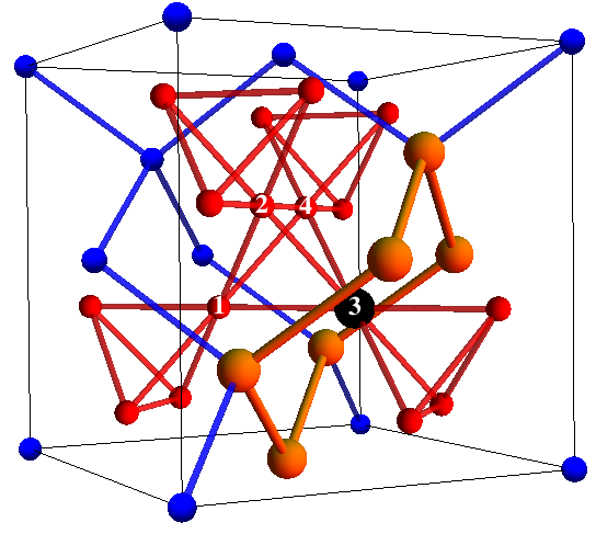
Figure 2: Impurity model: A non-magnetic impurity resides on a B-site indicated by the black sphere. The six nearest-neighbor A-sites form a distorted hexagon around the impurity.

In the following we investigate in detail one particular type of impurity relevant for the spinels, which brings out the general features of the problem. Specifically, we consider the effect of a magnetic ion on a B site of the spinel structure AB₂X₄. Each B-site atom has six nearest-neighbor A sites, and the distance in this case is smaller than the A-A nearest-neighbor distance. Thus, the dominant effect of this impurity is to generate an exchange coupling $J_{\rm imp}$ between the magnetic B-site and its six nearest-neighbor A-sites (see Figure 2), which is expected to be much stronger than the A-A exchange, i.e. $J_{\rm imp}\gg J_{1},J_{2}$. We therefore model a single B-site impurity by adding to the Hamiltonian the term

$$\delta H=J_{\rm imp}\sum_{\langle a,i\rangle}{\bf S}_{a}\cdot{\bf S}_{i},$$ (13)

where the sum is over the six A-site nearest neighbors $i$ to the B-site impurity labeled by $a$. Since we expect $J_{\rm imp}\gg J_{1},J_{2}$, the natural, simplest approximation is to take $J_{\rm imp}\rightarrow\infty$, in which case the impurity spin ${\bf S}_{a}$ can be eliminated and Eq. (13) reduces to a boundary condition that the six spins in the vicinity of the impurity are aligned.

It is noteworthy that the B-site does not have the full point group symmetry of the lattice. Instead there are four distinct B sites, which transform into one another under the full set of cubic operations (see Fig. 2). Therefore we must distinguish the four impurity positions within the unit cell, which we label $a=1,2,3,4$ in the energy function $E_{a}(q)$, as these will favor different ordered states.

II.2.3 Numerical results

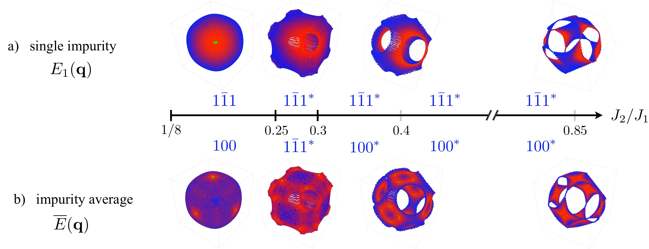
Figure 3: ‘Spiral surfaces’ comprising the degenerate spiral ground-state vectors for varying coupling strengths $J_{2}/J_{1}$. The surfaces are color-coded according to the energies $E_{1}({\bf q})$ and $E({\bf q})$, respectively. The colors indicate high values as blue, low values as red, and green being the absolute minima. The top row shows results for a single impurity $E_{1}({\bf q})$, while the bottom row shows results averaged over the four possible impurity sites $E({\bf q})$.

We have simulated the B-site impurity model numerically by employing extensive classical Monte Carlo simulations. We set up our simulations such that the impurity is embedded into systems of $N=8\times L^{3}$ spins with system sizes ranging up to $N=8\times 9^{3}=5832$ spins. In order to define the spiral state at large distances from the impurity site we employ fixed boundary conditions by embedding the simulation cube of length $L$ into a cube of extent $L+1$, where the spins in the boundary layer are aligned to form a uniform spiral of a given wavevector ${\bf q}$. In the vicinity of the impurity we consider the $J_{\rm imp}\rightarrow\infty$ limit and force the six nearest-neighbor spins of the impurity to be aligned and point in the same direction at all times in the simulations. We explore the zero temperature physics of this impurity model by setting the simulation temperature much lower than all energy scales in the problem, thereby mimicking a steepest descent energy minimization. We checked the convergence of this procedure by simulating systems with different initial spin configurations and obtained indistinguishable results when starting from random spin configurations or unperturbed spiral states, pointing to the existence of a unique (and well accessible) energy minimum.

Since the four distinct impurity sites within the diamond lattice unit cell are related by simple rotations, we have calculated the energy $E_{a}({\bf q})$ only for the impurity at one of these 4 sites. For a given value of interactions $J_{2}/|J_{1}|$ we have run simulations for a set of 1,000 distinct spiral wavevectors ${\bf q}$ on the ‘spiral surface’ appropriate for the value of couplings. A summary of our numerical results for a medium sized system of $N=512=8\times 4^{3}$ spins is plotted in the top row of Fig. 3. The impurity energies $E_{1}({\bf q})$ are found to vary on the spiral surfaces and clearly reflect the reduced symmetry of the single B site impurity problem. For instance, in the coupling range $1/8\leq J_{2}/|J_{1}|\leq 1/4$, where the spiral surface is a distorted sphere, the minimum energy wavevectors for $E_{1}(q)$ are ${\bf q}_{1}$ points which are along the $1\bar{1}1$ direction, while the energy for wavevectors in the $\bar{1}11$ direction (and others in the $\langle 111\rangle$ octet) is not an energy minimum.

For $J_{2}/|J_{1}|>1/4$, the spiral surface develops ‘holes’ centered around the $111$ directions and we find that $E_{1}({\bf q})$ develops three energy minima located symmetrically on the spiral surface along the $111^{*}$ direction for all couplings $J_{2}/|J_{1}|>1/4$ as indicated in the top row of Fig. 3.

Our numerical simulations also allow us to probe the spiral deformations in the vicinity of the impurity. In particular, we measure the local spiral wavevector ${\bf q}_{i}$ as described in detail in section II.2.1 using Eq. (12). Since we are mostly interested in estimating the deviation of this local wavevector ${\bf q}_{i}$ from the wavevector q for a given spin spiral configuration fixed at the boundary, we calculate the deviation $\delta q$ of the local spiral state defined as the angle between the spiral wavevectors ${\bf q}_{i}$ and q, e.g. $\cos{(\delta q)}={\bf q}_{i}\cdot{\bf q}/(|q||q_{i}|)$. Our results for the so-defined spiral deformation for various couplings and boundary spiral states are summarized in Fig. 4.

We find that the local rearrangement of spins in the vicinity of the impurity gives rise to a significant deviation of the (angle of the) local spiral wavevector of $O(1)$, while spins being separated from the impurity by about one unit cell spacing rearrange themselves in a spiral state which differs only marginally from the one fixed at the boundary. This short-range behavior of the spiral deviations is found to be quite insensitive to the size of the system and the distance from the fixed boundary configuration; for a more detailed discussion of finite-size effects see Appendix C.

We further analyze how the pattern of local wavevector deviations changes as we vary the couplings in the range $1/8<J_{2}/|J_{1}|<1/4$. This is shown in the two panels of Fig. 4 for fixed boundary spirals pointing in the $1\bar{1}1$ and $100$ directions, respectively. We see that the region of significant deformation of the spiral is in all cases restricted to the very close vicinity of the impurity, and varies only slightly with varying $J_{2}/J_{1}$.

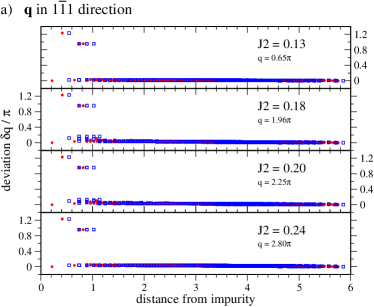
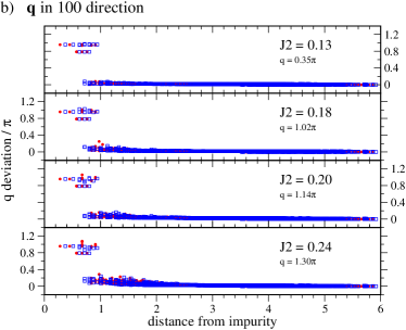
Figure 4: Deviation of the local spiral wavevector ${\bf q}_{i}$ from the one of the spiral state at the boundary $\bf q$. The left panel is for boundary spiral states with $\bf q$ pointing along the $1\bar{1}1$ direction in the coupling range $J_{2}/|J_{1}|<1/4$. The right panel is for boundary spiral states with $\bf q$ pointing along the $100$ direction in the coupling range $J_{2}/|J_{1}|<1/4$. The impurity is embedded into a system of $N=2,744=8\times 7^{3}$ spins. The symbols correspond to two different sets of neighboring spins, $P$ (circles) and $Q$ (boxes), used to calculate the local spiral wavevectors, details are given in the text.

III Dilute impurities

III.1 Ground state with many impurities

III.1.1 swiss cheese model

We turn now to the case of many impurities. We have seen that a single impurity already breaks the ground state degeneracy of the pure system, as well as the cubic symmetry of the crystal, thus favoring a unique state. However, the (four) different impurity positions within the unit cell break the cubic symmetry of the crystal in a different way, and hence each favors a different ordered state. For example, an impurity at one B-site will favors a spiral with wavevector along the $(111)$ direction, while another favors a wavevector along the $(11\overline{1})$ direction. In the physical system, equal densities of each type of impurity should be simultaneously considered.

Given that the four impurity types favor incompatible orders, what is the nature of the ground state that emerges here? We will address this question in the dilute limit, by which we mean that the impurity density $n_{\rm{imp}}$ is assumed to be much smaller than $\xi^{-3}$. One naive candidate ground state in this limit consists of domains such that around each defect the spins are close to a spiral with wavevector favored by that impurity type. However, this possibility can be dismissed since such a configuration would necessitate large scale deviations in wavevector between domains, which we have seen in Sec. II cost a prohibitively large energy. A more plausible outcome is that the ground state consists of a uniform spiral deformed locally around the defects, whose wavevector reflects a compromise between the different impurity types. Putting it more colloquially, the system looks like a “swiss cheese” (Emmentaler) with the bulk consisting of an ordered spiral and a set of holes in which the spins are strongly deformed about each impurity. In this case, since the energy is the sum of the energy shifts due to an equal number of each type of impurities, the ground state wavevector for the many-impurity case minimizes

$$E({\bf q})=\frac{1}{4}\sum_{a=1}^{4}E_{a}({\bf q}).$$ (14)

Eq. (14) constitutes a large simplification, justified by the impurity diluteness—the many-impurity ground state is determined from an average over single-impurity quantities. In this sense, the impurities in this limit act independently.

The above discussion asserts that the ground state away from the impurities is essentially undeformed on scales comparable to the impurity separation and somewhat larger. This is indeed a consequence of the assumption of dilute impurities and the locality arguments of Sec. II.1.2. However, this does not rule out the possibility that small deformations of the spiral on the scale of the impurity separation could add up on much longer distances to a larger deviation from long-range spiral order. We consider this carefully below. We find that the wavevector of the spiral indeed remains macroscopically uniform for dilute impurities, even on the longest scales, with small fluctuations. This is sufficient to guarantee the correctness of the energy estimate in Eq. (14), and hence correctly predict the wavevector favored by dilute impurities. The phase of the spiral, however, fluctuates considerably more, and our arguments suggest that there may be considerable reduction of the long-range ordered moment of the spiral by this mechanism.

To see this, we will construct a “coarse grained” energy function for the system containing many impurities, and consider the stability against perturbations to a macroscopically uniform spiral. We use the parametrization of an arbitrary slowly-varying deviation from a spiral state with wavevector ${\bf q}_{0}$ from Sec. II.1, in terms of the fields $\phi$ and $\psi$. The energy cost in the clean system for such a deviation is described by Eq. (10). We must add to this the impurity energy density,

$${\cal E}_{\rm imp}({\bf q}({\bf r}),{\bf r})=\sum_{a}E_{a}({\bf q}({\bf r}))n_{a}({\bf r}),$$ (15)

where the impurity density is

$$n_{a}({\bf r})=\sum_{{\bf R}_{a}}\delta({\bf r}-{\bf R}_{a}),$$ (16)

and ${\bf R}_{a}$ are the impurity positions. The impurity density is a random function. For long-wavelength properties, the central limit theorem implies that it is well-characterized by its first few moments. Taking the impurities to be uniformly and independently distributed over the system volume with a total average density $x$ (or $x/4$ per impurity type), we find the mean and two-point correlation

$$\overline{n_{a}({\bf r})} = x/4,$$ (17)

$$\overline{n_{a}({\bf r})n_{b}({\bf r}^{\prime})}-\overline{n_{a}({\bf r})}\;\overline{n_{b}({\bf r}^{\prime})} = \frac{x}{4}\delta({\bf r}-{\bf r}^{\prime})\delta_{ab},$$ (18)

in the infinite volume limit. From this, we can evaluate the mean and second cumulant of the impurity energy density. The mean is

$$\overline{{\cal E}_{\rm imp}({\bf q},{\bf r})}=xE({\bf q}).$$ (19)

This is precisely the energy in Eq. (14), and is, as expected, linearly proportional to the impurity concentration $x$.

As a consequence, the impurity-averaged energy is minimized by the spiral wavevectors that minimize $E({\bf q})$. To ascertain the stability of these minima in the impurity distribution we now turn to analyze fluctuations about the minima of $E({\bf q})$, parametrized as ${\bf q}={\bf q}_{0}+{\boldsymbol{\nabla}}\phi$ (this is the same slowly varying $\phi$ field from Section II.1.2). Consider fluctuations in the impurity energy

$$\delta{\cal E}_{\rm imp}({\bf q}({\bf r}),{\bf r})={\cal E}_{\rm imp}({\bf q}({\bf r}),{\bf r})-\overline{{\cal E}_{\rm imp}({\bf q}({\bf r}),{\bf r})},$$ (20)

and expand to linear order in $\phi$:

$$\delta{\cal E}_{\rm imp}({\bf q}({\bf r}),{\bf r})\approx\left[{\cal E}_{\rm imp}({\bf q}_{0},{\bf r})-E({\bf q}_{0})\right]-{\bf f}_{\rm imp}({\bf r})\cdot{\boldsymbol{\nabla}}\phi.$$ (21)

The first term in the brackets is $\phi$-independent and can be neglected. The second term represents a “random force”, given by

$${\bf f}_{\rm imp}({\bf r})=-\sum_{a}n_{a}({\bf r}){\boldsymbol{\nabla}}_{q}E_{a}({\bf q}_{0}).$$ (22)

Since $E({\bf q})$ has a minimum at ${\bf q}_{0}$, it has vanishing first order derivatives at this point. This also implies that $\overline{{\bf f}_{\rm imp}({\bf r})}\sim{\boldsymbol{\nabla}}_{q}E({\bf q}_{0})=0$. The second cumulant of the force is however non-zero:

$$\overline{f_{\rm imp}^{\mu}({\bf r})f_{\rm imp}^{\nu}({\bf r}^{\prime})}=x\Delta_{\mu\nu}({\bf q}_{0})\delta({\bf r}-{\bf r}^{\prime}),$$ (23)

with

$$\Delta_{\mu\nu}({\bf q}_{0})=\frac{1}{4}\sum_{a}\frac{\partial E_{a}({\bf q}_{0})}{\partial q_{\mu}}\frac{\partial E_{a}({\bf q}_{0})}{\partial q_{\nu}}.$$ (24)

$\Delta_{\mu\nu}$ is generally non-zero and positive unless ${\bf q}_{0}$ is a saddle point for all impurity types. This is not the case for our problem, but even if it were, it would only further strengthen the tendency of the system to order.

We are now in a position to consider the full energy function. Since $\psi$ does not couple to the impurities, we can neglect it. The energy density involving $\phi$ then combines the first terms in Eq. (10), the mean impurity contribution near a minimum of $E({\bf q})$ to quadratic order in $\phi$

$$\overline{{\cal E}_{\rm imp}({\bf q}({\bf r}),{\bf r})}\approx xE({\bf q}_{0})+\frac{x}{2}\frac{\partial^{2}E({\bf q}_{0})}{\partial q_{\mu}\partial q_{\nu}}\partial_{\mu}\phi\partial_{\nu}\phi,$$ (25)

and the random force from Eq. (21). Up to an unimportant additive constant, we find

$${\cal E} = \frac{c}{2}(\nabla_{\perp}\phi)^{2}+c^{\prime}\nabla_{\perp}\phi\nabla_{\parallel}^{2}\phi+\frac{c^{\prime\prime}}{2}(\nabla^{2}_{\parallel}\phi)^{2}$$ (26)

$$+\frac{x}{2}\frac{\partial^{2}E({\bf q}_{0})}{\partial q_{\mu}\partial q_{\nu}}\partial_{\mu}\phi\partial_{\nu}\phi-{\bf f}_{\rm imp}({\bf r})\cdot{\boldsymbol{\nabla}}\phi.$$

To proceed, we note that for dilute impurities (small $x$), the fourth term in Eq. (26) is much smaller than the first two except when considering the energy cost for gradients $\nabla_{\parallel}\phi$ parallel to the spiral surface, and therefore keep only these components. For simplicity, we will approximate these components as isotropic, and replace

$$\frac{\partial^{2}E({\bf q}_{0})}{\partial q_{\mu}\partial q_{\nu}}\partial_{\mu}\phi\partial_{\nu}\phi\rightarrow c_{\rm imp}(\nabla_{\parallel}\phi)^{2}.$$ (27)

It is now straightforward to minimize the energy in Eq. (26) in Fourier space:

$$\phi({\bf k})=\frac{-i{\bf k}\cdot\tilde{f}_{\rm imp}({\bf k})}{ck_{\perp}^{2}+c^{\prime}k_{\perp}k_{\parallel}^{2}+c^{\prime\prime}k_{\parallel}^{4}+xc_{\rm imp}k_{\parallel}^{2}}.$$ (28)

Finally, we can evaluate the local variance of the wavevector $\delta{\bf q}={\boldsymbol{\nabla}\phi}$:

$$\overline{\delta{\bf q}({\bf r})^{2}} = \int_{\bf k}k^{2}\overline{\phi({\bf k})\phi(-{\bf k})}$$

$$= x\Delta_{\mu\nu}\int_{\bf k}\frac{k^{2}k_{\mu}k_{\nu}}{(ck_{\perp}^{2}+c^{\prime\prime}k_{\parallel}^{4}+xc_{\rm imp}k_{\parallel}^{2})^{2}-(c^{\prime})^{2}k_{\perp}^{2}k_{\parallel}^{4}}.$$

To estimate the integral for small $x$, we note the denominator of the integrand vanishes more rapidly with $k_{\parallel}$ than with $k_{\perp}$, and hence the largest terms will be those in which the momenta in the numerator are taken in the $k_{\parallel}$ directions. Hence, up to angular factors which do not affect the scaling with $x$, we estimate

$$\overline{|\delta{\bf q}({\bf r})|^{2}}\sim x|\Delta|\int d^{2}k_{\parallel}dk_{\perp}\frac{k_{\parallel}^{4}}{(ck_{\perp}^{2}+c^{\prime\prime}k_{\parallel}^{4}+xc_{\rm imp}k_{\parallel}^{2})^{2}-(c^{\prime})^{2}k_{\perp}^{2}k_{\parallel}^{4}}.$$ (30)

The integral over $k_{\perp}$ can be performed directly to obtain

$$\overline{|\delta{\bf q}({\bf r})|^{2}}\sim x|\Delta|\frac{1}{\sqrt{c}}\int_{0}^{\Lambda}dk_{\parallel}\frac{k_{\parallel}^{2}}{(\tilde{c}^{{}^{\prime\prime}}k_{\parallel}^{2}+xc_{\rm imp})^{1/2}(c^{{}^{\prime\prime}}k_{\parallel}^{2}+xc_{\rm imp})},$$ (31)

where $\tilde{c}^{\prime\prime}=c^{\prime\prime}-(c^{\prime})^{2}/(4c)$, and we have introduced the radial momentum coordinate $k_{\parallel}$ and introduced a high momentum (short distance) cut-off $\Lambda$. The integral is readily seen to be logarithmically divergent for small $x$, hence

$$\overline{|\delta{\bf q}({\bf r})|^{2}}\sim\frac{|\Delta|x}{\sqrt{c}}\ln(1/x).$$ (32)

In the limit $x\rightarrow 0$ the fluctuations of the wavevector vanish, and therefore fluctuations never diverge. The wavevector is indeed expected to remain uniform over the entire system, with only small fluctuations for small $x$.

A more subtle question concerns the deformation of the phase $\phi$ rather than the wavevector, because two well-separated regions of the sample can become arbitrarily out of phase as small deformations of the spiral accumulate between them. A similar analysis to above gives

$$\overline{|\phi({\bf r})|^{2}} = \int_{\bf k}\overline{\phi({\bf k})\phi(-{\bf k})}$$

$$\sim x|\Delta|\frac{1}{\sqrt{c}}\int_{0}^{\Lambda}dk_{\parallel}\frac{1}{(\tilde{c}^{{}^{\prime\prime}}k_{\parallel}^{2}+xc_{\rm imp})^{1/2}(c^{{}^{\prime\prime}}k_{\parallel}^{2}+xc_{\rm imp})}.$$

The integral in this case is much more singular. For small $x$ it is dominated by small $k_{\parallel}$ and independent of $\Lambda$. By rescaling, one finds it is proportional to $1/x$, canceling the $x$ dependence of the prefactor:

$$\overline{|\phi({\bf r})|^{2}}\gtrsim\frac{|\Delta|}{c_{\rm imp}\sqrt{cc^{\prime\prime}}}.$$ (34)

Because Eq. (34) is independent of $x$, there is no particular reduction of the spatial variations of the spiral phase for dilute impurities. This is symptomatic of the “softness” of the degenerate spiral manifold.

Inspecting both Eqs. (34,32), we see that, although fluctuations do not become large for small $x$, they do become large for small $c$. Since $c$ vanishes on approaching the Lifshitz point $J_{2}/J_{1}=1/8$, we expect that the spiral ordering should become unstable to impurity deformations in the neighborhood of this part of the phase diagram. We return to this point in the Discussion.

III.1.2 Numerical results

We have argued above that dilute impurities basically act independently of each other and that they favor a unique ground-state wavevector which minimizes the energy $E({\bf q})$. As a consequence, it is straightforward to estimate the impurity average $E({\bf q})$ from our numerical calculations of $E_{a}({\bf q})$ for a single impurity in section II.2.3. Our results for the impurity averaged energies $E({\bf q})$ are summarized in the bottom row of Fig. 3. Note that while $E_{a}({\bf q})$ does not have the full point group symmetry of the lattice, cubic symmetry is restored when calculating the average $E({\bf q})$.

In particular, our numerical results allow us to determine the direction of the long-distance spiral wavevector favored by an ensemble of dilute impurities. For couplings $1/8<J_{2}/|J_{1}|<1/4$, multiple defects favor a long-distance spiral wavevector residing on the spiral surface along one of the $100$ directions. For couplings $J_{2}/|J_{1}|>1/4$ where the spiral surface develops ‘holes’ centered around the $111$ directions, we find that also the long-distance spiral wavevector favored by an ensemble of dilute impurities first jumps to the $1\bar{1}1^{*}$ direction for $1/4<J_{2}/|J_{1}|\lesssim 0.30$, and then continuously moves to the $100^{*}$ directions for $J_{2}/|J_{1}|\gtrsim 0.30$ as illustrated in Fig. 3.

III.2 Interplay between impurity and entropic effects

We have argued that at zero temperature, dilute impurities lift the spiral degeneracy inherent in the pure system, generating “order by quenched disorder”. As discussed above and in Ref. Bergman et al., 2007, entropy provides another degeneracy lifting mechanism at finite temperature via “thermal order by disorder”. The interplay between these mechanisms leads to interesting physics as we will now discuss. In particular, over a wide range of $J_{2}/J_{1}$, disorder and thermal fluctuations favor decidedly different ordered states; e.g., for $J_{2}/J_{1}=0.2$, thermal fluctuations favor the 111 directions while impurities prefer the 100 directions. In such cases, since entropic corrections giving rise to thermal order by disorder vanish as $T\rightarrow 0$, the system is expected to exhibit multi-stage ordering, from an impurity-driven phase at the lowest $T$ to an entropically stabilized phase at moderate $T$ to a disordered paramagnet at still higher $T$. As an aside, we note that other interactions beyond those considered in our model and/or quantum fluctuations can compete with impurity effects at low $T$, but may similarly lead to multiple phase transitions. If the energetic corrections coming from impurity or other effects are too large, however, then the entropically stabilized phase will be removed, leaving a single ordered state.

Another interesting effect arising from the interplay between entropy and disorder, which can be probed experimentally, pertains to the shift in transition temperature $T_{c}$ at which the system first orders. Roughly, should entropy and disorder favor the same state, then $T_{c}$ is expected to be enhanced relative to the pure system; otherwise a reduction is anticipated. To estimate this shift, we note that the transition is first-order and that at $T_{c}$ the free energies for the paramagnet and the ordered phase must equal,

$$f_{sp}\left(T_{c}\right)+x\delta F_{sp}\left(T_{c}\right)=f_{PM}\left(T_{c}\right)+x\delta F_{PM}\left(T_{c}\right).$$ (35)

Here, $x$ is the impurity concentration, $f_{sp}$ and $f_{PM}$ are the free energies for a clean system in the spiral phase and paramagnet, respectively, and $x\delta F_{sp}$ and $x\delta F_{PM}$ are the corresponding changes in free energy due to the impurities. For a well defined thermal order-by-disorder phase, an approximate derivation (see Appendix D) yields the following result

$$T_{c}-T_{c}^{*}=T_{c}^{*}x\frac{\left[E(q)\right]_{S}-E({\bf q}_{0})}{l^{*}}\;,$$ (36)

where $T_{c}^{*}$ is the (upper) ordering temperature for the clean system, $l^{*}$ is the latent heat density to go from the ordered phase to the paramagnetic one in the clean crystal, $S$ is the degeneracy (spiral) surface and ${\bf q}_{0}$ is the momentum favored by thermal order-by-disorder in the clean system. We defined the surface average

$$\left[E(q)\right]_{S}=\frac{\int_{{\bf q}\in S}d{\bf q}E({\bf q})}{\int_{{\bf q}\in S}d{\bf q}}.$$ (37)

The quantities determining the $T_{c}$ shift in Eq. (36) can be extracted from numerics. We find that the latent heat $l^{*}$ is roughly independent of $J_{2}/J_{1}$. However, there is significant dependence of the numerator in Eq. (36) on this ratio. This is plotted in Fig. 5. The $T_{c}$ tracks this quantity, and is thus sensitive to the degree of frustration.

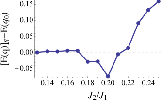
Figure 5: Plot of $\left[E(q)\right]_{S}-E({\bf q}_{0})$ versus frustration $J_{2}/J_{1}$. The shift of $T_{c}$ for the order-by-disorder phase per impurity is proportional to this quantity (see Eq. (36)).

IV Discussion

In this manuscript we have explored the effect of dilute impurities on the $J_{1}-J_{2}$ model on the diamond lattice. General considerations led us to conjecture that impurities may provide a mechanism for ground state degeneracy breaking. We established that, under rather general conditions, even highly frustrated magnets are induced to order by low concentrations of impurities. Moreover, the mechanism and energetics of this ordering was explained in terms of a simple “swiss cheese” picture. To expose the mechanism in more detail, we considered a very specific impurity model, namely B site magnetic ions being added to the system, and confirmed the general structure of the impurity-induced ordering by numerical and analytical means in this situation.

Let us briefly discuss this picture in relation to CoAl₂O₄ and MnSc₂S₄, the two A-site magnetic spinels exhibiting the largest frustration parameters without the complications of orbital degeneracy. Disorder in the form of inversion – A and B site atoms interchanging with one another – is prevalent in many spinels, including these, at the level of at least a few percent. One intriguing feature of the measurements on these materials is the observation of glassy freezing in CoAl₂O₄, but not in MnSc₂S₄, despite comparable levels of inversion in the two materials. This suggests that CoAl₂O₄ is more sensitive to defects than MnSc₂S₄, and our results corroborate this hypothesis. Theoretically, we argued that, generically, the effect of sufficiently dilute impurities is to induce order, not a spin glass. For the ordered state to be stable, we argued that: (1) the impurity “halos” should not overlap, and (2) the fluctuations in wavevector induced by the randomness of the impurity positions should be small. In Sec. III.1.1, we saw that the second criteria is highly sensitive to the magnitude of the stiffness $c$, the fluctuations becoming large as $c$ decreases. In the diamond lattice antiferromagnets, the stiffness $c$ actually vanishes on approaching the Lifshitz point $J_{2}/J_{1}=1/8$. Prior investigations concluded that in fact CoAl₂O₄ has exchange parameters close to this point, while in MnSc₂S₄, $J_{2}/J_{1}\approx 0.85$,Bergman et al. (2007) where $c$ is not small. Thus we suggest that the freezing behavior in CoAl₂O₄ may be understood as arising from proximity to the Lifshitz point. It may be interesting to directly study disorder physics in this region by field theoretic methods in the future.

We would like to emphasize the generality of this argument. The only assumption is that the impurity positions are not strongly correlated, but otherwise this conclusion is independent of the type of defects. Indeed, we do not maintain any direct relevance of the specific impurity modeled studied in the numerical portions of this paper to the A-site spinels. For CoAl₂O₄, the existence of magnetic ions on the B sites is probably suspect, as inverted Co⁺³ on the B sites would be expected to have a non-magnetic ground state. However, the expected spin “vacancies” induced by Al atoms on the A sites would lead to the same general conclusions. What would require a more appropriate microscopic model would be an estimate of the size of the region of deformed spins around an impurity.

Very recent experiments have greatly clarified the situation in CoAl₂O₄. Through a careful study of elastic and inelastic neutron scattering high quality single crystal, MacDougall et al. MacDougall et al. (2011) have argued that the freezing transition in CoAl₂O₄ signals an “arrested” first order transition in which the sample breaks up into antiferromagnetic domains. These domains are evidenced by a substantial Lorentzian-squared component to the elastic scattering. Moreover, below the freezing temperature spin-wave excitations were observed, a fit of which determined $J_{2}/J_{1}\approx 0.1$. This parameter ratio takes CoAl₂O₄ close to the Lifshitz point but $0.1<1/8$, so the commensurate Néel state would be expected at low temperature. The first order nature of the transition is consistent with theoretical expectations based on the order-by-disorder mechanism.Bergman et al. (2007) Given these exchange parameters, the detailed analysis of this paper does not directly apply, since we have assumed $J_{2}/J_{1}>1/8$ and focused on spiral ground states. However, arguments very similar to those we applied here to show a strong sensitivity to impurities close to the Lifshitz point on the spiral side also imply a similar sensitivity close to the Lifshitz point on the Néel side. Thus the findings are quite consistent with the general reasoning espoused here.

We conclude by describing an interesting feature of our numerical simulations, which might be of interest in future theoretical and experimental studies. We found that, while the ground states of the pure system are coplanar, the spin configuration around the impurity might acquire a sizable out-of-plane spin component, i.e. a spin component orthogonal to the plane in which the spin spiral state lies at long distances away from the impurity. This is in particular true for those spirals with wavevectors $\mathbf{q}$ such that their energies $E_{1}({\bf q})$ (see Eq.(B)) are far away from the overall minimum. It is possible that, collectively, impurities might therefore induce non-coplanar spin ordering. Such non-coplanar order is relatively rare, and interesting insofar as it can induce non-trivial Berry phases, related to anomalous Hall effects in conducting systems.

Appendix A Definition of local wavevector

Here we describe in detail how the local spiral wavevector is defined on the lattice, as used in Sec. II.2.3 and Figs. 4 and 6. Depending on the unperturbed spiral wavevector ${\bf q}$ taken at infinity we consider distinct sets of three neighboring sites out of the 12 second-neighbor sites which are nearest neighbors on the identical (fcc) sublattice. In particular, for ${\bf q}$ pointing in the $1\overline{1}1$ direction we consider two sets of vectors $\{{\bf r}_{ij}\}$, namely $P=\{(1/2,-1/2,0);(1/2,0,1/2);(0,-1/2,1/2)\}$ and $Q=\{(-1/2,-1/2,0);(1/2,0,-1/2);(0,-1/2,-1/2)\}$. For ${\bf q}$ pointing in the $100$ direction we consider two alternative sets of vectors $\{{\bf r}_{ij}\}$, namely $P^{\prime}=\{(1/2,1/2,0);(1/2,-1/2,0);(1/2,0,1/2)\}$ and $Q^{\prime}=\{(1/2,1/2,0);(1/2,0,1/2);(1/2,0,-1/2)\}$. We place the local wavevector ${\bf q}_{i}$ at position ${\bf r}_{i}-\frac{1}{4}\sum_{j=1}^{3}{\bf r}_{ij}$, which is always located inside the (convex) manifold spanned by the four spins.

Appendix B Symmetries

In this appendix, we give explicit expressions for the symmetry transformations and their effects, within our conventions for the spinel lattice. The space group is generated by the following operations:

1. A three-fold rotation about the $(1,1,1)$ axis:

   $$T_{1}:(x,y,z)\longrightarrow(z,x,y).$$ (38)

2. A two-fold rotation about the $(0,0,1)$ axis:

   $$T_{2}:(x,y,z)\longrightarrow(-x,-y,z).$$ (39)

3. Reflection through a $(1,-1,0)$ plane:

   $$T_{3}:(x,y,z)\longrightarrow(y,x,z).$$ (40)

4. Inversion:

   $$T_{4}:(x,y,z)\longrightarrow(\tfrac{1}{4}-x,\tfrac{1}{4}-y,\tfrac{1}{4}-z).$$ (41)

We define the following four impurity positions, ${\bf u}_{a}$ ($a=1,2,3,4$) modulo Bravais lattice transformations:

$${\bf u}_{1} =(3/8,5/8,3/8)\qquad{\bf u}_{2} =(3/8,3/8,5/8),$$ (42)

$${\bf u}_{3} =(5/8,3/8,3/8)\qquad{\bf u}_{4} =(5/8,5/8,5/8).$$

These positions are mapped into one another by the four space group generators. Corresponding to each of these generators is an associated linear transformation in reciprocal space. This transformation of wavevectors is identical to the transformation of real space coordinates except that translational components of the transformation are dropped. That is, if the coordinates transform according to ${\bf r}\rightarrow O{\bf r}+{\bf a}$ ($O$ is an O(3) matrix), then the corresponding momentum transformation is just ${\bf q}\rightarrow O{\bf q}$.

As a consequence, any given impurity position may be mapped to the other three by such an O(3) operation. One finds that (up to Bravais lattice vectors), the impurity positions transform according to

$$T_{a}{\bf u}_{b}={\bf u}_{c(b,a)},$$ (43)

where $c(a,b)$ can be represented as the matrix

$$c(a,b)=\left(\begin{array}[]{cccc}2&3&3&1\\ 3&4&2&2\\ 1&1&1&3\\ 4&2&4&4\end{array}\right),$$ (44)

where $a$ and $b$ specify the row and column of the matrix, respectively. We see from this that, for instance, an impurity on position 4 retains the symmetries generated by $T_{1}$, $T_{3}$ and $T_{4}$, but not $T_{2}$.

Moreover, we observe that each impurity position can be mapped to position 1 in the following way:

$${\bf u}_{1} = T_{1}\circ T_{1}\,{\bf u}_{2},$$ (45)

$${\bf u}_{1} = T_{1}\,{\bf u}_{3},$$ (46)

$${\bf u}_{1} = T_{1}\circ T_{1}\circ T_{2}\,{\bf u}_{4}.$$ (47)

This allows one to calculate the energies $E_{a}({\bf q})$ with $a=2,3,4$ from $E_{1}({\bf q}^{\prime})$ with an appropriate ${\bf q}^{\prime}$. Specifically

$$E_{2}(q_{x},q_{y},q_{z}) = E_{1}(q_{y},q_{z},q_{x}),$$

$$E_{3}(q_{x},q_{y},q_{z}) = E_{1}(q_{z},q_{x},q_{y}),$$

$$E_{4}(q_{x},q_{y},q_{z}) = E_{1}(q_{y},-q_{z},q_{x}).$$ (48)

Therefore, the average energy can be written as

$$E(q_{x},q_{y},q_{z}) = \frac{1}{4}\Big{[}E_{1}(q_{x},q_{y},q_{z})+E_{1}(q_{y},q_{z},q_{x})$$

$$+E_{1}(q_{z},q_{x},q_{y})+E_{1}(-q_{y},q_{z},-q_{x})\Big{]}.$$

We note that, taking into account the subgroup of the full space group which leaves position 1 invariant, the first impurity energy obeys

$$E_{1}(-q_{y},-q_{z},q_{x})=E_{1}(q_{z},q_{y},q_{x})=E_{1}(q_{y},q_{z},-q_{x})$$ (50)

$$=E_{1}(-q_{z},-q_{y},-q_{x})=E_{1}(q_{x},-q_{z},-q_{y})=E_{1}(q_{z},-q_{x},-q_{y})$$

$$=E_{1}(-q_{x},q_{z},q_{y})=E_{1}(-q_{z},q_{x},q_{y})=E_{1}(q_{x},q_{y},q_{z})$$

$$=E_{1}(-q_{y},-q_{x},q_{z})=E_{1}(-q_{x},-q_{y},-q_{z})=E_{1}(q_{y},q_{x},-q_{z}).$$

The average energy, by construction, has the full cubic space group symmetry, i.e.

$$E(q_{x},q_{y},q_{z})=E(s_{a}q_{a},s_{b}q_{b},s_{c}q_{c}),$$ (51)

where $s_{a},s_{b},s_{c}=\pm 1$ and $(q_{a},q_{b},q_{c})$ is an arbitrary permutation of $q_{x},q_{y},q_{z}$. As a consequence, $1/48$th of the solid angle in ${\bf q}$ space is enough to recover the full function $E({\bf q})$. We therefore carry out numerical simulations only for such a section, which we choose, arbitrarily, to be the one defined by:

$$(q_{x}>0)\wedge(q_{y}>0)\wedge(q_{z}>0)\wedge(q_{x}>q_{y})\wedge(q_{x}<q_{z})\,.$$

All points defined by Eq. (B) are inequivalent to one another, and conversely, can used to generate $E({\bf q})$ for an arbitrary point using Eq. (51).

Appendix C Locality of spin deformation and finite-size effects

Our numerical simulations of the B-site impurity model indicate that the deformation of the spin spiral state in the vicinity of the impurity is limited to a small numbers of spins in the unit cell around the impurity. Our numerical calculations are performed in an $L\times L\times L$ simulation cube embedded in a larger cube of extent $L+1$, where the spins in the ‘boundary cube’ are fixed to a particular spin spiral state. One might thus wonder whether the locality of the spin spiral deformation originates from the impurity physics, as opposed to artifacts due to the fixed boundary conditions. To exclude the latter we have calculated the spiral deviation for different system sizes $L$ and positioning of the impurity site, as summarized in Fig. 6 where we fix the boundary spiral wavevector to the $1\bar{1}1$ direction, which minimizes $E_{1}({\bf q})$ for the chosen ratio of couplings $J_{2}/|J_{1}|=0.2$. We find that the deviation is insensitive to varying the system size as shown in the various panels. Further, we also do not find a striking change of our results when embedding the impurity into a system of even extent $L=4$ (second panel from top in Fig. 6), which places the impurity site rather asymmetrically with respect to the fixed boundary spiral.

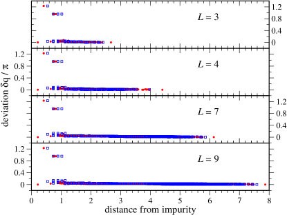
Figure 6: Finite size effects: Deviation of the local spiral wavevector ${\bf q}_{i}$ from the one of the spiral state at the boundary $\bf q$ for systems of varying size $N=8\times L^{3}$. For the chosen couplings $J_{2}/|J_{1}|=0.2$ the spiral wavevector ${\bf q}$ points along the $1\bar{1}1$ direction with length $|{\bf q}|=0.71\pi$. The symbols correspond to two different sets of neighboring spins, $P$ (circles) and $Q$ (boxes), used to calculate the local spiral wavevectors, details are given in the text.

Appendix D Derivation of the transition temperature shift

In this appendix we consider the transition between the high temperature paramagnetic phase, and an ordered phase where the spins order in a spiral configuration with a wavevector selected by entropy. We explore how adding impurities shifts the transition temperature, assuming that the impurities themselves do not change the nature of the ordered state. Quantities in the clean limit are denoted by a star.

For a first-order phase transition, at the transition temperature:

$$\begin{array}[]{l}f_{sp}\left(T_{c}\right)+x\delta F_{sp}\left(T_{c}\right)=f_{PM}\left(T_{c}\right)+x\delta F_{PM}\left(T_{c}\right)\\ f_{sp}\left(T_{c}^{*}\right)=f_{PM}\left(T_{c}^{*}\right),\end{array}$$ (53)

where $f_{sp,PM}$ are the free energy densities of the spiral phase and paramagnetic phase, respectively, and similarly $\delta F_{sp,PM}$ refer to the free energy density corrections when impurities are included. A small impurity concentration will only slightly shift the transition temperature, and so we expand the free energy density to first order in the temperature shift

$$\begin{split}f(T_{c})\approx&f(T_{c}^{*})+\frac{\partial f(T_{c}^{*})}{\partial T}(T_{c}-T_{c}^{*})\\ =&f(T_{c}^{*})+s(T_{c}^{*})(T_{c}-T_{c}^{*})\\ =&f(T_{c}^{*})+\left(f(T_{c}^{*})-\epsilon\right)\left(\frac{T_{c}}{T_{c}^{*}}-1\right)\;,\end{split}$$ (54)

where $s(T)$ is entropy, and $\epsilon$ is the energy density. From this we find

$$\left(\epsilon_{PM}-\epsilon_{sp}\right)\left(\frac{T_{c}}{T_{c}^{*}}-1\right)=x\left(\delta F_{PM}(T_{c})-\delta F_{sp}(T_{c})\right)\;.$$ (55)

Now we turn to estimate the free energy densities $\delta F$, which can be estimated from $F=-T\log{Tr\left[e^{-\beta H}\right]}$, when varying the Hamiltonian by a small term $x\delta H$. This will yield a small change in the free energy

$$\begin{split}&\delta F=-T\log{\left[\frac{Tr\left[e^{-\beta(H+\delta H)}\right]}{Tr\left[e^{-\beta H}\right]}\right]}\\ &\approx-T\log{\left[1-\beta\langle\delta H\rangle\right]}\approx+\langle\delta H\rangle\;,\end{split}$$ (56)

where the angle brackets denote a thermal average. Each impurity will contribute a term of the form of (13) to $\delta H$. Next we estimate the energy thermal average in each phase. In the ordered phase, the system remains mostly in the ground state configuration, and so we estimate $\delta F_{sp}\approx E({\bf q}_{0})$, where $E({\bf q})$ is the same as in (15), and ${\bf q}_{0}$ is the spiral wavevector. In the paramagnetic phase, close to the transition temperature, the system thermally fluctuates mostly amongst the different spiral states (this has been shown explicitly for the clean system in Ref. Bergman et al., 2007) and so we estimate $\delta F_{PM}\approx\int_{{\bf q}\in S}d{\bf q}E({\bf q})/(\int_{{\bf q}\in S}d{\bf q})$ where $S$ is the spiral surface. We find therefore

$$\left(\epsilon_{PM}-\epsilon_{sp}\right)\left(\frac{T_{c}}{T_{c}^{*}}-1\right)=x\left(\frac{\int_{{\bf q}\in S}d{\bf q}E({\bf q})}{(\int_{{\bf q}\in S}d{\bf q})}-E({\bf q}_{0})\right)\;,$$ (57)

and finally

$$T_{c}-T_{c}^{*}=\frac{T_{c}^{*}x}{l^{*}}\left(\frac{\int_{{\bf q}\in S}d{\bf q}E({\bf q})}{(\int_{{\bf q}\in S}d{\bf q})}-E({\bf q}_{0})\right)\;,$$ (58)

where $l^{*}=\left(\epsilon_{PM}-\epsilon_{sp}\right)$ is the latent heat density to go from the order-by-disorder phase to the paramagnetic phase in a clean system.

References

- Moessner and Ramirez (2006) R. Moessner and A. P. Ramirez, Physics Today 59 (2006).
- Villain et al. (1980) J. Villain, R. Bidaux, J. P. Carton, , and R. Conte, J. de Phys. 41 (1980).
- Henley (1989) C. L. Henley, Phys. Rev. Lett. 62, 2056 (1989).
- Bergman et al. (2006) D. L. Bergman, R. Shindou, G. A. Fiete, and L. Balents, Phys. Rev. B 74, 134409 (2006).
- Bergman et al. (2007) D. Bergman, J. Alicea, E. Gull, S. Trebst, and L. Balents, Nature Physics 3, 487 (2007).
- Yamashita and Ueda (2000) Y. Yamashita and K. Ueda, Phys. Rev. Lett. 85, 4960 (2000).
- Bramwell and Gingras (2001) S. T. Bramwell and M. J. P. Gingras, Science 294, 1495 (2001).
- Gvozdikova and Zhitomirsky (2005) M. V. Gvozdikova and M. E. Zhitomirsky, JETP Letters 81 (2005).
- Chalker et al. (1992) J. T. Chalker, P. C. W. Holdsworth, and E. F. Shender, Phys. Rev. Lett. 68, 855 (1992).
- Reimers et al. (1991) J. N. Reimers, A. J. Berlinsky, and A.-C. Shi, Phys. Rev. B 43, 865 (1991).
- Shender et al. (1993) E. F. Shender, V. B. Cherepanov, P. C. W. Holdsworth, and A. J. Berlinsky, Phys. Rev. Lett. 70, 3812 (1993).
- Ramirez (1994) A. P. Ramirez, Annual Review of Materials Science 24, 453 (1994).
- Fritsch et al. (2004) V. Fritsch, J. Hemberger, N. Buttgen, E.-W. Scheidt, H.-A. K. von Nidda, A. Loidl, and V. Tsurkan, Phys. Rev. Lett. 92, 116401 (2004).
- Tristan et al. (2005) N. Tristan, J. Hemberger, A. Krimmel, H.-A. K. von Nidda, V. Tsurkan, and A. Loidl, Phys. Rev. B 72, 174404 (2005).
- Krimmel et al. (2006) A. Krimmel, M. Mucksch, V. Tsurkan, M. M. Koza, H. Mutka, C. Ritter, D. V. Sheptyakov, S. Horn, and A. Loidl, Phys. Rev. B 73, 014413 (2006).
- MacDougall et al. (2011) G. J. MacDougall, D. Gout, J. L. Zarestky, G. Ehlers, A. Podlesnyak, M. A. McGuire, D. Mandrus, and S. E. Nagler, e-print (2011), eprint arXiv:1103.0049.
- Giri et al. (2005) S. Giri, H. Nakamura, and T. Kohara, Phys. Rev. B 72, 132404 (2005).
- Grinstein and Pelcovits (1982) G. Grinstein and R. A. Pelcovits, Phys. Rev. A 26, 915 (1982).
- Albuquerque et al. (2007) A. Albuquerque, F. Alet, P. Corboz, P. Dayal, A. Feiguin, S. Fuchs, L. Gamper, E. Gull, S. Guertler, A. Honecker, et al., J. Magn. Magn. Mater. 310, 1187 (2007).