Massive stars in the Cl 1813-178 Cluster. An episode of massive star formation in the W33 complex.

Abstract

Young massive ($M>10^{4}$ M_⊙) stellar clusters are a good laboratory to study the evolution of massive stars. Only a dozen of such clusters are known in the Galaxy. Here we report about a new young massive stellar cluster in the Milky Way. Near-infrared medium-resolution spectroscopy with UIST on the UKIRT telescope and NIRSPEC on the Keck telescope, and X-ray observations with the Chandra and XMM satellites, of the Cl 1813-178 cluster confirm a large number of massive stars. We detected 1 red supergiant, 2 Wolf-Rayet stars, 1 candidate luminous blue variable, 2 OIf, and 19 OB stars. Among the latter, twelve are likely supergiants, four giants, and the faintest three dwarf stars. We detected post-main sequence stars with masses between 25 and 100 M_⊙. A population with age of 4-4.5 Myr and a mass of $\sim 10000$ M_⊙ can reproduce such a mixture of massive evolved stars. This massive stellar cluster is the first detection of a cluster in the W33 complex. Six supernova remnants and several other candidate clusters are found in the direction of the same complex.

1 Introduction

An understanding of the mechanisms of formation, evolution, and end state of massive stars is fundamental for the studies of galaxies at all redshifts. Massive stars contribute to the chemical enrichment of the interstellar medium with their strong winds and by exploding as supernovas. Massive stars are the most luminous stars, can easily be detected in external galaxies, and provide distance estimates. They are the sources of the most energetic phenomena in the Universe, gamma ray bursts (e.g. Woosley & Bloom, 2006).

The availability of large surveys of the Galactic plane at radio and infrared wavelengths opens a golden epoch for studying the formation, evolution, and environments of massive stars. More than 1500 new candidate stellar clusters have been discovered, and among them several young clusters rich in massive stars may be hidden (Messineo et al., 2009).

In Messineo et al. (2008) (hereafter referred to as PaperI), we presented the serendipitous discovery of a young massive cluster, Cl 1813-178, in the Galactic disk at l=12^∘, with a spectroscopically identified population of massive stars, a red supergiant star (RSG), two blue supergiants (BSG), and one Wolf-Rayet (WR) star. Here, we present a follow-up study of the cluster. Near-infrared photometry and spectroscopy, and X-ray observations, reveal a large number of massive stars.

The cluster is located in the W33 complex, and is associated with two supernova remnants (SNR), SNR G12.72$-$0.00 and G12.82$-$0.02, and the highly magnetized pulsar associated with the TeV $\gamma$-ray source HESS J1813$-$178. Interestingly, the W33 complex appears to contain several other candidate stellar clusters, and several SNRs. Clusters do form in large complexes (e.g. Beuther et al., 2007), and their spatial distribution varies from cloud to cloud, indicating that several external and internal triggers can be at work (e.g. Clark et al., 2009). W33 is an ideal laboratory to investigate various issues about massive stars and multi-seeded star formation, and to verify the presence of triggered sequential star formation, which is suggested by the presence of SNRs. The association of the stellar cluster with two SNRs can shed light on the initial masses of the supernova progenitors, and on the fate of massive stars.

We describe the observations and data reduction in Sect. 2, and we analyze the spectra and the cluster color-magnitude diagram (CMD) in Sect. 3. A discussion on the massive members and spectrophotometric distances is presented in Sects. 4 and 5. Cluster age and mass are derived in Sects. 6 and 7. An overview of candidate clusters in the direction of the W33 complex is given in Sect. 8. Finally, our findings are summarized in Sect. 9.

2 Observations and data reduction

2.1 IR photometry

Photometric measurements from the near-infrared Two Micron All Sky Survey (2MASS) catalog (Skrutskie et al., 2006), the Galactic Legacy Infrared Mid-Plane Survey Extraordinaire (GLIMPSE) catalog (Benjamin et al., 2003), as well as from the Naval Observatory Merged Astrometric Dataset (NOMAD) (Zacharias et al., 2004) were used.

Images of the central cluster region with the $J$, $H$ and K_s filters were obtained during two nights of observation, 2008 June 23-24, using the near-IR camera SofI mounted on the ESO NTT (Moorwood et al., 1998). We used SofI in large-field mode with a pixel size of 0.288^′′, and a total field of view of 4.9’$\times$4.9’. For each filter, we performed a random dithering pattern of 14 images, and reached a total exposure time of 840s, 1176s, and 1680s in $J$, $H$ and K_s, respectively. Each image is a combination of 50, 70, and 100 exposures, each one 1.2 s long, in $J$, $H$, and K_s bands, respectively.

Data reduction was performed using standard IRAF routine. For each filter, we obtained a sky image by median-combining the dithered frames, and we subtracted the sky image from each frame, Flat fielding was performed by using the SpecialDomeFlat template, which applies the appropriate illumination correction, as described in the SofI User Manual. Finally, the dithered frames were averaged into a single image. Standard crowded-field photometry, including point-spread function modeling, was carried out on each image using DAOPHOT II/ALLSTAR (Stetson 1987). The internal photometric accuracy was estimated from the rms frame-to-frame scatter of multiple star measurements (0.03 mag$<{\sigma}_{J}$${\sim}{\sigma}_{H}{\sim}{\sigma}_{K_{s}}<$0.06 mag for 8$<J{\sim}H{\sim}K_{s}<$18). The instrumental magnitudes were converted into the 2MASS photometric system. The 2MASS catalog was used as an astrometric reference frame. For stars that were saturated on the SofI images, magnitudes were taken from the 2MASS catalog.

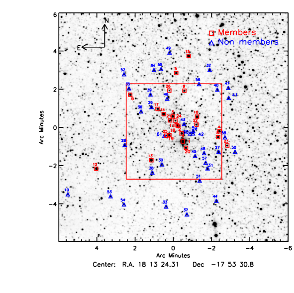
Figure 1: 2MASS K_s-band image of the cluster. The big box shows the location of the field observed with SofI. Stars that were spectroscopically observed and are likely cluster members are marked with small boxes. Non-member stars are marked with triangles.

2.2 Near-IR spectroscopy

Spectroscopic observations of the brightest stars were carried out with NIRSPEC at the Keck Observatory under program H243NS (PI: Kudritzki) on 2008 July 24. The K-filter and a 42^′′$\times$ 0.570^′′ slit were used, covering from 2.02 to 2.45 $\mu$m with a resolution of R=1700. For each target, two nodded exposures of 10s each were taken. We observed a total of 23 stars with NIRSPEC (see Tables 1 and 7).

Additional spectroscopic data were taken with the UKIRT 1-5 micron Imager Spectrometer (UIST) at the UKIRT Observatory . We used the short-K grism in combination with a 120^′′$\times$ 0.12^′′ slit, covering from 2.00 to 2.26 $\mu$m at a resolution R=1800. We also used the long-K grism to cover the spectral range from 2.204 to 2.513 $\mu$m at a resolution of R=1900. Typically, each target was observed with the long-K grism. When CO bands were not detected, a second spectrum was taken with the short-K grism. Integration times varied from 30 to 60 s per exposure, and the number of exposures varied from 8 to 20 s. The 39 stars observed with UKIRT, including a few chance detections, are listed in Tables 1 and 7.

Pairs of frames with nodded positions were subtracted and flat-fielded. The stellar traces were straightened using a two dimensional de-warping procedure. We wavelength calibrated the spectra with arc lines. We corrected the spectra for atmospheric absorption and instrumental response by dividing the observed spectra by the spectrum of a reference star. Reference stars were of B type (from B2 to B9). The Br$\gamma$ and HeI lines of the telluric spectrum were eliminated with linear interpolation.

The signal to noise of the spectra varied from 40 to 150.

2.3 X–ray data

The cluster is located in the vicinity of the HESS J1813-178 pulsar wind nebula (Helfand et al., 2007). Several X-ray observations of this region have been performed in order to identify the pulsar associated with the HESS source. Helfand et al. (2007) presented a catalog of 75 point sources detected with the Chandra satellite. We cross-correlated the Chandra catalog with the 2MASS point source catalog, and identified a total of 44 matches (PaperI). Using the XMM satellite, Funk et al. (2007) detected seven X-ray sources in the surrounding area of HESSJ1813-178.

3 Analysis

3.1 Spectral classification

Spectral classification was performed by comparing the spectra with spectral atlases (e.g. Hanson et al., 1996, 2005; Figer et al., 1997; Martins et al., 2007; Kleinmann & Hall, 1986; Wallace & Hinkle, 1996).

We observed a total of 60 stars, and detected 24 early-type stars and 36 late-type stars. In addition, we considered the previous observations reported in PaperI, which added an extra early-type star (#11) to our new sample. The observed stars were divided into candidate cluster members and non members, and are listed in Tables 1, and 7. We first listed the sample of stars given in the Table 1 of PaperI, using the same identification numbers, then we appended the new targets ordered in K_s magnitude. The spectra of the newly detected early-type stars are shown in Figs. 2, and 3.

In the following, we describe the spectra by grouping the stars into late-types and early-types. Early types divided in four subgroups (Wolf-Rayet stars, candidate luminous blue variables, O-type, and B-type stars).

3.1.1 Red Supergiants

In the K-band, the spectra of late-type stars have CO band-heads at 2.29 $\mu$m. By measuring the equivalent widths of the CO bands, it is possible to distinguish between giants and supergiants (see the Appendix).

Among the detected late-type stars, four stars, #1, #32, #38, and #39, are found to have equivalent widths of the CO bands, EW(CO), typical of RSGs.

Star #1 is a K2-K5I cluster member, as discussed in PaperI on the basis of high-resolution data.

Star #32, #38, and #39 have EW(CO)s typical of RSGs with spectral types M2.5, M3.5 and M1, respectively. Their photometric properties indicate that they are unrelated to the stellar cluster. We further discuss these stars in the following sections.

3.1.2 Wolf-Rayet stars

Star #4 is a known WR star of type WN7 (number #8 in Hadfield et al., 2007). Star #7 has similar emission lines at 2.114 $\mu$m, 2.166 $\mu$m, and 2.189 $\mu$m. By comparing it with the spectral atlas of Figer et al. (1997), star #7 appears to be another WN7 star (see Fig. 4).

3.1.3 Candidate Luminous Blue Variables

The spectrum of star #15 is dominated by He I lines at 2.058 $\mu$m  and 2.112 $\mu$m, and Br$\gamma$ line in emission. Faint MgII lines are detected at 2.138 $\mu$m and 2.144 $\mu$m. The type of detected lines and the line profiles indicate that star #15 is a P-Cygni B supergiant. Its spectrum is similar to that of the candidate luminous blue variable (cLBV) star in the W51 region (Clark et al., 2009). More information on the stellar photometric variability is needed to firmly confirm that it is another LBV star.

3.1.4 O-type stars

Spectra of O and B stars have hydrogen lines, helium lines, and other atomic lines (e.g. CIV, NIII, CIII, MgII). Hydrogen and helium lines are usually seen in absorption; they may be in emission in supergiants. The Br$\gamma$ line is the only hydrogen line detectable in K-band. The HeI transitions at 2.058$\mu$m and 2.112 $\mu$m are usually detected in late-O and early-B stars. The HeII line at 2.189 $\mu$m appears only in O-type stars. With our resolution, the HeII line at 2.189$\mu$m  may be present down to O9.5I or O9V.

The spectrum of star #6 has a strong HeI line at 2.058 $\mu$m in absorption, CIV lines at 2.069 $\mu$m and 2.079 $\mu$m in emission, strong emission line at 2.11 $\mu$m (probably due to HeI/NIII/CIII), and a HeII absorption line at 2.189 $\mu$m. NIII at 2.25$\mu$m is seen in emission. There is an indication for a faint CIV line at 2.083 $\mu$m, and a NIII line at 2.10 $\mu$m. The simultaneous presence of HeI, HeII, and CIV lines is typical of an O-type star. The strengths of the HeI and HeII absorption lines, as well as the detection of NIII at 2.25$\mu$m, indicate a O6-O7f+.

The spectrum of star #16 has Br$\gamma$ line in emission, a HeI line at 2.058 $\mu$m with P-Cygni profile, and a HeI/NIII line at 2.112 $\mu$m. A HeII line at 2.189 $\mu$m is seen in absorption. A faint line is seen in emission at 2.105 $\mu$m. Only an indication for a CIV line at 2.08 $\mu$m is visible. The spectrum resembles that of a O8-O9If star, similar to HD151804 (Morris et al., 1996).

Stars #18, #19, and #20 have HeI lines at 2.058 and 2.112 $\mu$m in absorption, a NIII line at 2.115 $\mu$m in emission, and Br$\gamma$ line in absorption. A HeII line at 2.189 $\mu$m clearly appears in absorption. The absence of CIV lines, and the presence of NIII and HeII lines, suggest a late O-type (O7-09).

The spectra of stars #5, #8, and #9 have HeI lines at 2.058 $\mu$m, and 2.112 $\mu$m in absorption, and Br$\gamma$ line in absorption. There is an indication for a NIII line at 2.115 in emission, and a HeII line at 2.189 $\mu$m in absorption. Star #5 has a clear detection of a NIII line. The absence of CIV lines, and the presence (or indication) of NIII and HeII lines, suggest that this is a late O-type (O7-O9).

3.1.5 B-type stars

Here, we list all detected early-type stars, which do not have HeII lines. These may be B-stars or O9 dwarfs. With our resolution, the HeII line at 2.189$\mu$m  may be present down to O9.5I or O9V. Once the HeII line disappears, assigning a spectral type and luminosity class can turn into a quite degenerate issue. This degeneracy may be partly broken if the absorption components of the Br$\gamma$ line and of the HeI lines are sufficiently filled in by the stellar wind contribution. Typically, a HeI line at 2.112$\mu$m in absorption is observed down to B8Ia stars, while the same line is not detected in dwarfs/giants later than B3V. Such matters are highly dependent on the quality of the spectra.

From a comparison with the atlas of Hanson et al. (1996), stars #2, #3, #11, #12, #13, #14, #17, #21, #22, #23, #24, #25, and #26 appear to be likely stars with types from B0 to B2.

The spectra of stars #2 and #13 have a HeI line at 2.058 $\mu$m  in emission, a HeI line at 2.112 $\mu$m, and Br$\gamma$ line in absorption. From the relative strengths of the Br$\gamma$ and HeI lines (Hanson et al., 1996), the presence of HeI in emission at 2.058$\mu$m, and the lack of HeII lines, these stars appear to be B0-B3 supergiants.

The spectra of stars #3, #22, #24 , #25, and #26 have a HeI line at 2.112 $\mu$m  in absorption, as well as Br$\gamma$ line in absorption. Star #17 has Br$\gamma$  line in absorption, and a trace of HeI at 2.112$\mu$m. These are likely B0-B3 stars or O9-B3 stars (depending on the luminosity class).

The spectra of stars #11, #21, and #23 have Br$\gamma$  line in absorption, HeI lines at 2.058 and 2.112 $\mu$m  in absorption. These spectra are typical of early B-type stars.

Star #12 has Br$\gamma$  line in absorption. The lack of HeI al 2.112 in absorption suggests that star #12 has a spectral type later than a B8I or B3-B4V star.

The spectrum of star #14 has Br$\gamma$ in absorption, a HeI line at 2.112 $\mu$m  in absorption, an indication for a HeI line in emission at 2.058 $\mu$m, and a faint HeI line at 2.113 $\mu$m in emission. The lack of HeII at 2.189$\mu$m and presence of HeI lines suggest that star #14 is a BSG star with spectral type between B0 and B3.

The spectrum of star #11 is shown in PaperI. Stars #2 and #3 were also observed with NIRSPEC in April 2008 (PaperI), and we obtained the same spectral classification.

Table 1: List of cluster members spectroscopically observed.

ID	Ra	Dec	B	V	R	J	H	Ks	[3.6]	[4.5]	[5.8]	[8.0]	tel.	Sp
1	18 13 22.26	-17 54 15.55	14.74	13.68	12.73	5.46	4.23	3.79	5.07	4.05	3.57	$\cdots$	keck	RSG
2	18 13 23.26	-17 53 26.54	20.08	15.03	14.50	8.64	7.72	7.22	6.94	6.78	6.63	6.68	keck	B0-B3
3	18 13 24.43	-17 52 56.75	20.42	15.74	14.68	9.20	8.25	7.79	7.47	7.38	7.30	7.30	keck	B0-B3
4	18 13 14.19	-17 53 43.60	20.48	17.57	15.20	9.62	8.60	7.94	7.34	6.93	6.70	6.35	keck	WN7
5	18 13 23.71	-17 50 40.41	19.51	16.41	14.94	9.96	9.06	8.56	8.23	8.10	7.99	8.06	keck	O7-O9
6	18 13 33.82	-17 51 48.89	$\cdots$	$\cdots$	16.12	10.29	9.15	8.57	8.00	7.90	7.75	7.75	ukirt	O6-O7f
7	18 13 22.52	-17 53 50.14	18.63	15.60	16.57	10.30	9.27	8.66	8.03	7.70	7.49	7.30	ukirt	WN7
8	18 13 14.49	-17 54 01.77	19.91	15.47	15.71	9.86	9.12	8.75	8.43	8.33	8.31	8.31	ukirt	O7-O9
9	18 13 21.91	-17 51 35.91	21.17	$\cdots$	16.24	10.74	9.80	9.34	8.95	8.90	8.83	8.91	ukirt	O7-O9
11	18 13 23.62	-17 53 24.46	$\cdots$	$\cdots$	$\cdots$	11.74	10.85	9.59	10.16	10.32	10.02	99.99	keck	B0-B3
12	18 13 41.33	-17 55 41.14	$\cdots$	17.42	18.09	9.07	7.50	6.75	6.41	6.31	5.87	5.95	keck	B9-A2
13	18 13 29.18	-17 55 14.55	21.09	$\cdots$	15.66	8.79	7.56	6.85	6.80	6.15	6.03	5.99	keck	B0-B3
14	18 13 26.47	-17 52 49.48	16.27	14.25	13.01	8.21	7.38	6.91	6.81	6.44	6.38	6.32	keck	B0-B3
15	18 13 20.98	-17 49 46.88	19.67	$\cdots$	15.40	8.93	7.78	6.96	6.76	5.91	5.71	5.42	keck	cLBV
16	18 13 19.13	-17 52 57.43	$\cdots$	$\cdots$	16.90	9.43	8.10	7.33	6.94	6.47	6.40	6.19	keck	O8-O9If
17	18 13 27.83	-17 52 33.19	$\cdots$	13.46	13.13	9.70	8.97	8.52	8.29	8.23	8.16	8.20	keck	B0-B3
18	18 13 25.25	-17 53 55.05	20.13	16.60	14.02	10.05	9.05	8.61	8.25	8.09	7.96	8.04	ukirt	O7-O9
19	18 13 25.20	-17 53 55.83	19.49	16.28	16.20	10.25	9.25	8.72	8.41	8.25	8.21	8.20	ukirt	O7-O9
20	18 13 21.54	-17 54 35.65	$\cdots$	$\cdots$	$\cdots$	10.60	9.61	9.14	8.70	8.62	8.49	8.59	ukirt	O7-O8
21	18 13 25.06	-17 53 09.34	$\cdots$	16.84	13.98	10.73	9.78	9.29	9.03	8.86	8.85	8.77	ukirt	O9-B3
22	18 13 19.25	-17 53 22.62	$\cdots$	$\cdots$	$\cdots$	11.42	10.10	9.34	8.76	8.57	8.40	8.50	ukirt	O9-B3
23	18 13 12.47	-17 54 28.26	19.01	15.37	13.95	10.65	9.83	9.44	9.19	9.21	9.10	9.14	ukirt	O9-B3
24	18 13 23.87	-17 53 10.10	$\cdots$	$\cdots$	$\cdots$	11.68	10.75	10.31	9.96	9.89	9.80	9.91	ukirt	O9-B3
25	18 13 25.90	-17 53 57.45	$\cdots$	$\cdots$	20.28	12.33	11.34	10.82	10.48	10.45	10.25	10.46	ukirt	O9-B3
26	18 13 25.23	-17 51 35.64	15.37	14.90	$\cdots$	13.64	11.74	10.84	10.16	10.12	10.00	10.07	ukirt	O9-B3

Note. — For each star, number designations and coordinates (J2000) are followed by magnitudes measured in different bands. J,H, and K_s measurements are from 2MASS, while the magnitudes at 3.6 $\mu$m, 4.5 $\mu$m, 5.8 $\mu$m, and 8.0 $\mu$m are from GLIMPSE. $B$, $V$, and $R$ associations are taken from the astrometric catalog NOMAD.

Figure 2: K-band spectra of early-type stars obtained with NIRSPEC on the Keck telescope. The full line shows the spectrum after correction for atmospheric absorption and instrumental response, and interstellar extinction. Extinction correction was performed with the values listed in Table 2, and by assuming a power law with an index of $-$1.9 (Messineo et al., 2005). The dashed line shows a black body with a temperature equal to the stellar effective temperature. Each spectrum was normalized at 2.12 $\mu$m, and arbitrarily shifted for clarity. The locations of detected spectral lines are indicated with marks and labels.

Figure 3: K-band spectra of early-type stars obtained with UIST on the UKIRT telescope. Curves and labels are as in Fig. 2

.

Figure 4: Spectra of star #4, which is an already known WR star (Hadfield et al., 2007), and star #7, which is a newly detected WR star. For comparison, a spectrum of a WN7 star, WR120, is presented from the atlas of Figer et al. (1997). The rest wavelengths of HeII, HeI, HI, and CIII/NIII lines are also marked.

3.2 Photometric results

3.2.1 Cluster size

We assume as a cluster center the flux weighted centroid of a 2MASS K_s-band smoothed image (RA=18:13:24.15, DEC=-17:53:29.64). We take as a cluster radius the average distance from the cluster center where the surface brightness becomes equal to the average brightness of the surrounding field (3.5^′). The 61 spectroscopically observed stars are located within 6.5^′ from the cluster center, but predominantly (50) within the cluster radius. Within 3.5^′ from the cluster center, we observed 41 stars out of the 48 stars with K_s$<9.5$ mag, and 30 stars out of the 31 stars with K_s$<9.0$ mag.

A fraction of 48% of stars brighter than K_s=9.5 mag, within the cluster radius, have early types, and are likely to be members. The high degree of completeness of the spectroscopic observations of the bright sample allows for a precise numbering of stars in various post-main sequence phases (WR, cLBV, RSG, and OB stars).

3.2.2 Color-Magnitude Diagram and cluster reddening

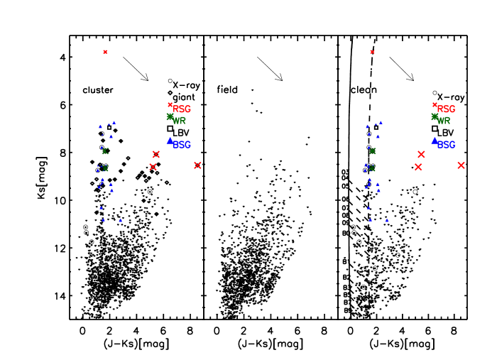
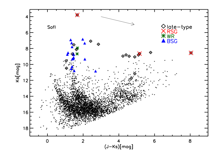
Figure 5: Left upper panel: A 2MASS $J-$K_s versus K_s  diagram of point sources detected within 3.5^′ from the cluster center is displayed. Middle upper panel: For comparison, A CMD for stars taken from a surrounding annulus (with a minor radius of 7^′ and area equal to that of the cluster) is show. Right upper panel: A CMD of the cluster field after statistical decontamination is shown. The vertical line indicates an isochrone of 4.5 Myr, with solar metallicity, and with a distance of 4.8 kpc (solid) (Lejeune & Schaerer, 2001); the same isochrone shifted to a reddening of A${}_{\rm K_{\rm s}}$=0.83 mag is indicated with a dashed line. The locations of OB stars on the ZAMS with A${}_{\rm K_{\rm s}}$=0 mag are marked with labels; dashed lines show their paths to A${}_{\rm K_{\rm s}}$=0.83 mag. The arrow indicates the reddening vector for A${}_{\rm K_{\rm s}}$=1 mag, based on the extinction law by Messineo et al. (2005). Stars spectroscopically observed are marked with special symbols, as listed in the legend. Bottom: $J-$K_s versus K_s diagram of point sources detected in the SofI images. Symbols are the same as in the upper panels.

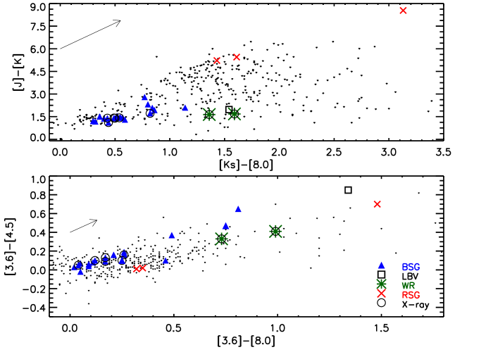
Figure 6: Upper panel: K_s$-[8.0]$ versus $J-$K_s diagram of point sources detected within 3.5^′ from the cluster center. The arrow indicates the reddening vector for A${}_{\rm K_{\rm s}}$$=1.0$ mag, which is calculated by following a near-infrared power law with $\alpha=$1.9 (Messineo et al., 2005), and by using the extinction ratios $A_{3.6}$/A${}_{\rm K_{\rm s}}$, $A_{4.5}$/A${}_{\rm K_{\rm s}}$, $A_{5.8}$/A${}_{\rm K_{\rm s}}$, $A_{8.0}$/A${}_{\rm K_{\rm s}}$of Indebetouw et al. (2005). Symbols are as seen in Fig. 5. Bottom panel: GLIMPSE [3.6]-[8.0] versus [3.6]-[5.8] diagram of point sources detected within 3.5^′ from the cluster center. Symbols and arrow are as shown in the top panel.

In the top panels of Fig. 5, we display a ($J-$K_s) vs. K_s diagram of 2MASS data points within the cluster radius of 3.5^′, as well as a diagram of a comparison field. The same CMD with deeper SofI data, covering the central 4.9^′$\times$4.9^′, is shown in the bottom panel of Fig.  5.

Several distinct populations of stars are seen in the CMD. There is a sequence of stars at $J-$K_s=0.5 mag, which we attribute to field stars in the closer Sagittarius-Carina spiral arm. There is a broad sequence with $J-$K_s from 3 to 6 mag, which is populated mainly by field giant stars in the background of the cluster. Three candidate RSGs were detected from this sequence. Finally, there is a sequence of bright stars with $J-$K_s$=\sim 1.5$ mag and with K_s from 3 to 14 mag (bottom panel of Fig.  5). This sequence is seen only in the cluster field, and this is the brightest extension of the cluster sequence.

To confirm and isolate the cluster sequence, we performed a statistical decontamination. 2MASS data were used in order to have a comparison field. We counted the number of stars in a grid of 0.5 mag in ($J-$K_s) and of 1.0 mag in K_s. From each bin of the cluster CMD, we subtracted a number of stars equal to that of the corresponding field bin. First, we subtracted all contaminating giant stars (spectroscopically detected), then we continued with a random subtraction. The decontaminated diagram is displayed in the right panel of Fig. 5, and different symbols indicate known spectral types. The cluster sequence appears populated by massive stars. An average interstellar extinction of A${}_{\rm K_{\rm s}}$$=0.83\pm 0.2$ mag (Av$=9.1$ mag) was estimated by matching the colors of the observed cluster sequence with a theoretical isochrone of solar composition from the Geneva group (Lejeune & Schaerer, 2001), and by assuming a power–law extinction curve A_λ $\propto\lambda^{-1.9}$ (Messineo et al., 2005). This measurement is independent of age since the isochrones are almost vertical sequences in this plane. An isochrone of 4.5 Myr and solar metallicity, taken from the non-rotating models of the Geneva group, is over-plotted on the diagram (Lejeune & Schaerer, 2001).

4 Luminosities of the massive stars

In the following, we analyze the properties (colors, magnitudes, and luminosities) of massive stars in the Cl 1813-178 cluster, which we list in Table 2. A kinematic distance of 4.8 kpc is used (see below the RSG section). For each star, we assumed an intrinsic color consistent with its stellar spectral type (Koornneef, 1983; Martins & Plez, 2006; Wegner, 1994); we used the extinction law by Messineo et al. (2005), and the kinematic distance, and we estimated a value of A${}_{\rm K_{\rm s}}$ and M_K  (see Table 2). The M_K values were transformed into bolometric magnitudes, Mbol, by adding the bolometric corrections. The adopted effective temperatures and bolometric corrections per spectral type are given in the Appendix.

4.1 Red supergiants

Star #1 is the brightest star within the cluster area, K_s=3.8 mag, and is consistent with being a K2-K5 I cluster member (PaperI). From the radial velocity ($V_{LSR}=62\pm 4$) of star #1 (PaperI), and the Galactic rotation curve by Reid et al. (2009), we obtained a revised near kinematic distance of $4.8^{+0.25}_{-0.28}$ kpc. With intrinsic colors from Koornneef (1983), bolometric correction, BC_K, taken from Levesque et al. (2005), we estimated a luminosity L_∗$=9\pm 7\times 10^{4}$ L_⊙.

Stars #32, #38, and #39 have EW(CO)s larger than the typical values for red giants. Stars #32 and #38 were observed with NIRSPEC, and their $K$-band spectral coverage allows us to study both the CO band heads, and the shape of the continuum. The large values of EW(CO)s and the absence of water absorption suggest a supergiant luminosity class for stars #32 and #38 (Comeron, 2004). Star #39 was observed with UIST on UKIRT, with the $K-$long filter only, and we do not have information on the shape of its continuum. We derived spectral types M2.5I, M3.5I, and M1I, respectively, by assuming a supergiant luminosity class for all three stars.

Stars #32, #38, and #39 are among the brightest stars with red $J-$K_s (from 3 to 9 mag), much redder than the cluster sequence as shown in Figs.  5, and 6. By assuming intrinsic $H-$K_s and $J-$K_s colors for a given spectral type (see the Appendix), we obtained A${}_{\rm K_{\rm s}}$= 2.3 mag, 3.6 mag, and 2.3 mag, respectively. These values of interstellar extinction are the combined contribution of interstellar and possible circumstellar extinction (Messineo et al., 2005). By analyzing the distribution of detected stars in the $Ks-[8.0]$ vs $J-$K_s plane (6), star #38 appears to show an excess in $Ks-[8.0]$, which is suggestive of a circumstellar envelope. Stars #32, and #39 have $Ks-[8.0]$ and $J-$K_s colors in agreement within errors with those of naked late-type stars (Messineo et al., 2004, 2005). We corrected for the total extinction by using the intrinsic colors for given spectral types and the extinction law by Messineo et al. (2005). We then artificially reddened the stars to emulate the average cluster condition. By assuming these stars were moved along the reddening vector to the average cluster extinction (A${}_{\rm K_{\rm s}}$=0.8 mag), we obtained K_s=6.7 mag, 5.8 mag, and 7.2 mag, respectively.

If these RSGs were at the same distance as the stellar cluster they should be the brightest stars at near-infrared wavelengths, and their K_s magnitudes would increase with later spectral types. Their spectral types are later than the bright (K_s=3.8 mag) K2I star, and their de-reddened magnitudes are similar to those of the brightest OB stars (K_s$=\sim 7$ mag). The spectral types and magnitudes of these three RSGs are not consistent with cluster membership; they are too faint to be RSGs and part of the cluster. This reasoning is valid also for stars with moderate mass-loss, i.e. #38, because bolometric corrections BC_K  are almost constant for colors K_s$-[8.0]<3$ mag (chapter5, Figs. A1 and A2, Messineo, 2004).

We estimated a density of non-member RSGs equal to 0.16 in the central 3.5^′. These RSGs could represent an outburst farther away, perhaps related to the Galactic bar.

4.2 Wolf Rayet stars

Star #4, a WN7b, was spectroscopically detected by Hadfield et al. (2007). Hadfield et al. performed a successful color-based selection of candidate WR stars with 2MASS and GLIMPSE data. WRs have an infrared excess (see Figs. 6 and 5), which is caused by free-free emission, and do not follow the reddening vector. Star #7 is a newly detected WN7o star, its colors fall within the Hadfield et al. criteria.

For stars #4 and #7, we used intrinsic colors for WN stars with broad and narrow lines, respectively, derived by Crowther et al. (2006a) (see the Appendix). We obtained an interstellar extinction A${}_{\rm K_{\rm s}}$=0.7 mag, and A${}_{\rm K_{\rm s}}$=0.8 mag, respectively. By adopting the kinematic distance, BC_K from Crowther et al. (2006a), we obtained L_∗$=5.8\pm 2.5\times 10^{5}$ L_⊙ for star #4, and L_∗$=4.8\pm 2.1\times 10^{5}$ L_⊙ for star #7.

4.3 Luminous blue variables

Among the observed spectra, we detected one candidate cLBV star (#15). LBV stars are rare massive supergiants in transition towards the Wolf-Rayet phase (e.g. Conti et al., 1995; Nota et al., 1995; Figer et al., 1997; Conti, 1984). Since their evolutionary paths on the CMD are quite uncertain, their detections in stellar clusters are of primary importance. The K-band spectrum of star #15 is similar to that of a P Cygni-type B supergiant, cLBV, e.g. the [OMN2000]LS1 star presented by Clark et al. (2009). We used CMFGEN, the iterative non-LTE line blanketing method presented by Hillier & Miller (1998), to estimate the physical properties of this supergiant. For details on the modeling see Najarro et al. (1999), Najarro (2001) and Clark et al. (2009).

The K-band spectra provided the primary diagnostics (the HeI lines at 2.058 $\mu$m and 2.112 $\mu$m, and the MgII lines at 2.138 $\mu$m and 2.144 $\mu$m). We obtained an effective temperature T${}_{eff}=\sim 16,000\pm 300$ k, and a value of L_∗$=2.1\pm 1.5\times 10^{5}$ L_⊙. This value matches the luminosities of the faintest P-Cygni supergiants known in the Milky Way (Clark et al., 2005, 2009).

4.4 OB stars

We detected 21 OB stars in the Cl 1813-178 cluster. The current dataset of medium-resolution K-band spectra allow for a spectral classification of OB stars typically within $\pm$2 spectral types (Hanson et al., 1996). The combination of spectral and photometric properties suggests that we have detected 14 OB supergiants, 4 OB giants, and 3 OB main sequence stars.

For star #6 (O6-O7If+), when using an intrinsic ($H-$K_s)${}_{0}=-0.1$ mag, and BC_K=$-4.01$ mag (Martins & Plez, 2006), we obtained M_K=$-$5.87 mag and L_∗$=8.2\pm 2.3\times 10^{5}$ L_⊙. The estimated value of M_K is consistent with the value given for an O6-O7 star by Martins & Plez (2006) and Clark et al. (2005).

Star #16 is another rare O supergiant, an O8-O9If type. By assuming ($H-$K_s)${}_{0}=-0.1$ mag, and BC_K=$-3.84$ mag (Martins & Plez, 2006), we obtained M_K=$-7.32$ mag and L_∗$=23\pm 6\times 10^{5}$ L_⊙. Star #16 is the brightest early-type cluster member, and it is located close to the observed Humphreys-Davidson limit for stars with similar effective temperatures (Clark et al., 2005).

From a comparison with the M_K values by Martins & Plez (2006) and Panagia (1973), the OB stars #25, #24, and #26 are likely dwarfs, since they have M_K$\leq-4$ mag (L_∗$\leq 1.4\times 10^{5}$ L_⊙). The OB stars #9, #21, #22, and #23 are probably of luminosity classes III or II, since they are fainter than a typical BSG. Their M_K values range from $-$4.7 to $-$5.36 mag (L_∗ varies from $1.1\times 10^{5}$ to $1.5\times 10^{5}$ L_⊙). All remaining OB stars are supergiants.

The large spread in magnitudes of OB supergiants ($\sim 3$ mag in K_s-band) is not surprising. A similar observational spread is observed in the 2MASS K_s magnitudes of BSGs in Westerlund 1 (Clark et al., 2005).

Table 2: Derived properties of stellar members.

ID	Ks	J-Ks	H-Ks	EJ-Ks	EH-Ks	AK	MK	Lum	log(Teff[K])	Sp. type	Class
1	3.79	1.67	0.44	1.02	0.31	0.54$\pm$ 0.13	-10.16	4.95 ${}^{0.24}_{-0.25}$	3.60 ${}^{0.01}_{-0.02}$	RSG	I
2	7.22	1.42	0.50	1.50	0.54	0.80$\pm$ 0.02	-6.99	5.70 ${}^{0.34}_{-0.34}$	4.31 ${}^{0.12}_{-0.12}$	B0B3	I
3	7.79	1.41	0.46	1.49	0.50	0.79$\pm$ 0.02	-6.41	5.46 ${}^{0.34}_{-0.34}$	4.31 ${}^{0.12}_{-0.12}$	B0B3	I
4	7.94	1.68	0.66	1.31	0.39	0.69$\pm$ 0.05	-6.16	5.76 ${}^{0.16}_{-0.17}$	4.70 ${}^{0.04}_{-0.05}$	WN7	I
5	8.56	1.40	0.50	1.61	0.60	0.87$\pm$ 0.02	-5.72	5.75 ${}^{0.12}_{-0.13}$	4.50 ${}^{0.03}_{-0.03}$	O7O9	I
6	8.57	1.72	0.58	1.93	0.68	1.03$\pm$ 0.02	-5.87	5.92 ${}^{0.11}_{-0.12}$	4.54 ${}^{0.02}_{-0.02}$	O6O7If	I
7	8.66	1.64	0.61	1.51	0.50	0.80$\pm$ 0.05	-5.55	5.68 ${}^{0.16}_{-0.17}$	4.70 ${}^{0.04}_{-0.05}$	WN7	I
8	8.75	1.11	0.37	1.32	0.47	0.71$\pm$ 0.01	-5.36	5.61 ${}^{0.12}_{-0.13}$	4.50 ${}^{0.03}_{-0.03}$	O7O9	I
9	9.34	1.40	0.46	1.61	0.56	0.86$\pm$ 0.02	-4.93	5.47 ${}^{0.13}_{-0.14}$	4.51 ${}^{0.03}_{-0.03}$	O7O9	III
11	9.59	2.15	1.26	2.23	1.30	1.37$\pm$ 0.02	-5.19	4.98 ${}^{0.34}_{-0.34}$	4.31 ${}^{0.12}_{-0.12}$	B0B3	III
12	6.75	2.32	0.75	2.23	0.74	1.19$\pm$ 0.02	-7.85	5.07 ${}^{0.13}_{-0.14}$	3.98 ${}^{0.03}_{-0.03}$	B9A2	I
13	6.85	1.94	0.71	2.02	0.75	1.08$\pm$ 0.03	-7.64	5.96 ${}^{0.34}_{-0.34}$	4.31 ${}^{0.12}_{-0.12}$	B0B3	I
14	6.91	1.30	0.47	1.38	0.51	0.74$\pm$ 0.02	-7.24	5.79 ${}^{0.34}_{-0.34}$	4.31 ${}^{0.12}_{-0.12}$	B0B3	I
15	6.96	1.97	0.82	1.99	0.84	1.09$\pm$ 0.02	-7.53	5.38 ${}^{0.22}_{-0.23}$	4.20 ${}^{0.01}_{-0.01}$	LBV	I
16	7.33	2.10	0.77	2.31	0.87	1.24$\pm$ 0.01	-7.32	6.36 ${}^{0.11}_{-0.12}$	4.48 ${}^{0.01}_{-0.01}$	O8O9If	I
17	8.52	1.18	0.45	1.26	0.49	0.68$\pm$ 0.03	-5.56	5.13 ${}^{0.34}_{-0.34}$	4.31 ${}^{0.12}_{-0.12}$	B0B3	I
18	8.61	1.44	0.44	1.65	0.54	0.88$\pm$ 0.05	-5.67	5.74 ${}^{0.13}_{-0.14}$	4.50 ${}^{0.03}_{-0.03}$	O7O9	I
19	8.72	1.53	0.53	1.74	0.63	0.94$\pm$ 0.02	-5.62	5.72 ${}^{0.12}_{-0.13}$	4.50 ${}^{0.03}_{-0.03}$	O7O9	I
20	9.14	1.46	0.47	1.62	0.51	0.86$\pm$ 0.03	-5.13	5.58 ${}^{0.11}_{-0.12}$	4.54 ${}^{0.01}_{-0.01}$	O7O8	I
21	9.29	1.44	0.49	1.60	0.57	0.86$\pm$ 0.03	-4.98	5.04 ${}^{0.38}_{-0.38}$	4.36 ${}^{0.13}_{-0.13}$	O9B3	III
22	9.34	2.08	0.76	2.24	0.84	1.22$\pm$ 0.03	-5.28	5.16 ${}^{0.38}_{-0.39}$	4.36 ${}^{0.13}_{-0.13}$	O9B3	III
23	9.44	1.21	0.39	1.34	0.42	0.71$\pm$ 0.02	-4.67	5.03 ${}^{0.30}_{-0.30}$	4.39 ${}^{0.11}_{-0.11}$	O9B3	III
24	10.31	1.37	0.44	1.50	0.47	0.79$\pm$ 0.02	-3.89	4.72 ${}^{0.30}_{-0.30}$	4.39 ${}^{0.11}_{-0.11}$	O9B3	V
25	10.82	1.51	0.52	1.64	0.55	0.88$\pm$ 0.04	-3.46	4.55 ${}^{0.30}_{-0.30}$	4.39 ${}^{0.11}_{-0.11}$	O9B3	V
26	10.84	2.80	0.90	2.93	0.93	1.55$\pm$ 0.02	-4.12	4.81 ${}^{0.30}_{-0.30}$	4.39 ${}^{0.11}_{-0.11}$	O9B3	V

4.5 X–ray emitters

Table 3: Massive stars with X-ray emission.

ID	Ks	Sp. Type	IdCh	CountsCh	HR	IdXMM	CountsXMM	Lx
	[mag]							[$10^{31}$ erg s-1]
2	7.22	OB	39	14.10	$-$0.33	$\cdots$	$\cdots$	4.1
3	7.79	OB	43	16.40	$-$0.53	$\cdots$	$\cdots$	4.8
4	7.94	WR	24	272.40	0.78	2	238	80.5
5	8.56	OB	41	214.50	0.42	4	138	63.4
6	8.57	OB	58	13.60	$-$0.57	$\cdots$	$\cdots$	4.0
7	8.66	WR	37	34.90	0.89	$\cdots$	$\cdots$	10.3
8	8.75	OB	27	13.00	$-$0.82	$\cdots$	$\cdots$	3.8
9	9.34	OB	36	9.50	$-$0.20	$\cdots$	$\cdots$	2.8
10	9.60	K	71	71.10	$-$0.31	$\cdots$	$\cdots$	21.0

Note. — For each star, number designations, K_s magnitudes, and spectral types from Tables 1 and 7 are followed by the number designations (ID_Ch), counts (counts), and hardness (HR) from the Chandra observations by Helfand et al. (2007), and by the number designations (Id_XMM) and XMM counts reported by Funk et al. (2007). Estimates of L_X are taken from PaperI, and assume a distance of 4.7 kpc, N(H)=$1.6\times 10^{22}$ cm^-2, a power-law model, and a photon index of 1.5. X–ray luminosities are given in units of $10^{31}$ erg s^-1.

X-ray emission may be generated in the circumstellar envelopes of massive stars due to their strong shocked winds (Lucy & White, 1980). Single OB stars emit with a typical X-ray luminosity of L_X= 10^31-33 erg s^-1 (Pollock, 1987), and have a typical ratio between the X-ray and bolometric luminosities of about $10^{-7}$. OB+OB and OB+WR binaries generally have higher luminosities (L_X$=10^{32-35}$ erg s^-1, Clark et al., 2008). X-ray emission enables us to characterize the physical condition of stellar atmospheres, and to identify binary systems.

X-ray observations of the Cl 1813-178 cluster region were performed by Funk et al. (2007) and Helfand et al. (2007), successfully detecting a large number (75) of X-ray emitters. We looked for possible associations between X-ray emitters and massive members of the Cl 1813-178 cluster (PaperI). All but one X-ray sources with a bright 2MASS counterpart (K_s$<9.6$ mag), were found associated with early-type cluster members (see Table 3). Two X-ray emitters coincide with WR stars (#4 and #7); six others are associated with OB stars (#2, #3, #5, #6, #8, and #9). The remaining X-ray emitter (#71, Helfand et al., 2007) coincides with star #10, which is likely a cluster non-member. This star is located 6.6^′  from the cluster center, outside of the cluster radius (3.5^′). Its spectrum has CO bands at 2.29 $\mu$m, which indicate a late-type star.

We estimated the ratios between the X-ray and bolometric luminosities, and we compared the ratio, hardness and X-ray luminosities of our nine X-ray emitters with those of Chandra point sources detected in Westerlund 1 (Fig. 5 Clark et al., 2005). In Westerlund 1, WR stars have luminosities L_X larger than $10^{32-34}$ erg s^-1 and hardness from $-0.1$ to 1, while most of the detected OB stars have L_X=10³² erg s^-1 (which is consistent with a ratio of $\sim 10^{-7}$) and hardness between $-0.8$ and $-0.1$, as expected for single stars with shocked winds. Clark et al. suggest that all OB stars with X-ray emission significantly harder than $-$0.5 in Westerlund 1 are binary systems. This conclusion is supported by emerging evidence of a high-binary fraction of massive stars in Westerlund 1 (Bonanos, 2007). Skinner et al. (2010) propose a number of other possible scenarios to explain the X-ray emission of single WN stars. Magnetic wind confinement could also explain the presence of a hot plasma component without invoking the presence of a close companion. However, current detections of magnetic fields in WN stars are absent.

Star #4, a WN7 star, is the brightest X-ray emitter. It is associated with the Chandra source #24 (Helfand et al., 2007), and coincides also with the XMM source #2 of Funk et al. (2007). The ratio between the X-ray and bolometric luminosities of star #4 is $3.7\times 10^{-7}$. For star #7, we obtained a ratio 7 times fainter. Both ratios are consistent with those measured in other WN stars by Skinner et al. (2010). Their high values of hardness (0.78 and 0.89 in Table 3) are consistent with those of colliding wind binaries (Clark et al., 2008). Since only a few other late WN stars have been detected in X–ray (Skinner et al., 2010), our new detections are a significant addition.

Star #5 (O7-O9) was detected by both the XMM and Chandra satellites (see Table 3). It is a strong X-ray emitter (L_X$=1\times 10^{32}$ erg s^-1); the ratio between the X–ray and bolometric luminosities is $2.9\times 10^{-7}$. Besides the two WR stars, star #5 is the only other source with a strong X-ray hardness (0.4). The high values of X-ray luminosity and hardness indicate that #5 is another binary.

For the BSGs #2 and #3 (B0-B3), we measured ratios between the X-ray and bolometric luminosities of $2.1-4.3\times 10^{-8}$, which are in agreement with the ratios measured for single stars later than B1 (Cohen, 1996; Waldron & Cassinelli, 2007). Stars #8 and #9 (O7-O9) have also a ratio of about $2.5\times 10^{-8}$.

For star #6, an O6O7If, we estimated a ratio of $1.3\times 10^{-8}$. The low ratio and low hardness ($-$0.57) suggest radiative shocks in stellar winds.

5 Spectro-photometric distances

Massive evolved stars in a young stellar cluster span a range of masses (see Fig. 7), therefore, of luminosities. Spectro-photometric distances from OB supergiants are less accurate than those from dwarfs and giants. When considering the dwarfs and the M_K magnitudes for O9, B0, B1, and B2 dwarfs (Martins & Plez, 2006; Humphreys & McElroy, 1984; Koornneef, 1983), we estimated distances of $3.8\pm 0.6$ kpc, $3.2\pm 0.5$ kpc, $2.6\pm 0.4$ kpc, and $1.9\pm 0.3$, respectively.

From the photometric properties of the candidate giants (#9, #21, #22, and #23), and M_K values for classes II and III from Humphreys & McElroy (1984) and Wegner (1994), we derived an average spectro-photometric distance of $3.0\pm 0.7$ kpc for class III, or $4.5\pm 0.6$ for class II.

For the two WN7 stars, we adopted intrinsic magnitudes from Crowther et al. (2006a), and the extinction law by Messineo et al. (2005), and obtained a distance of $2.6$ kpc for star #4, and $5.8$ kpc for star #7. The average distance for the two WN7 stars is $4.2\pm 1.6$ kpc.

The derived spectrophotometric distances are listed in Table 4. While the distance estimates from giants and WRs within errors are consistent with the kinematic distance, the distance estimates from dwarfs are only consistent with the kinematic distance if the dwarfs are all late O stars. Higher-resolution spectra are needed to refine the spectral types.

Table 4: Average spectrophotometric distances

Sp. type	distance
OB V	$2.9\pm 0.8$
OB III/II	$3.8\pm 1.0$
WN7	$4.2\pm 1.6$
average	$3.6\pm 0.7$

Observations of radio hydrogen recombination lines of the W33 complex reveal two velocity components (Bieging et al., 1978; Goss et al., 1978). By using the radial velocity component at 35 km s^-1, and the rotation curve of Reid et al. (2009), we calculated a near kinematic distance of $3.53^{+0.40}_{-0.46}$ kpc, while we obtained a distance of $4.82^{+0.25}_{-0.28}$ kpc with the radial velocity component at 62 km s^-1. A radio monitoring program of methanol masers in the direction of the W33 complex is currently ongoing. It will yield parallactic distances of the masers (Brunthaler et al. in preparation).

6 Progenitor masses and the cluster age

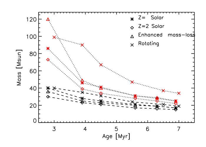
Figure 7: For a given age, the mass at the TO and the maximum mass predicted by models are shown. Several models are used: a model by Schaller et al. (1992) with a solar metallicity (asterisks), models with metallicity twice solar by Schaerer et al. (1993) (diamonds), models with high mass-loss by Meynet et al. (1994) (triangles), and the rotating models by Meynet & Maeder (2000) (crosses). For each model, the maximum masses are connected with a dotted line, while the masses at the TO are connected with a dashed line.

The Cl 1813-178 cluster contains a large number of evolved massive stars (BSGs, a cLBV, two WN7 stars, and one RSG star), which are listed in Table 1. We plot the inferred stellar luminosities versus stellar effective temperatures in Fig.  8, together with theoretical stellar models from the Geneva group (Meynet & Maeder, 2000). By comparison with the models, we estimated initial masses from 20 to 100 M_⊙.

Models predict a large span of stellar masses in post main sequence phase, e.g. a population of 4.0 Myr would have a mass of 25-35 M_⊙ at a TO, but it would still contain stars of about 50M_⊙, or even 100 if rotating models are considered. This is well illustrated in Figure 7, where we show the predicted maximum initial masses and TO masses as a function of cluster age. We used non-rotating models by Schaller et al. (1992) and Schaerer et al. (1993), models with high-mass loss by Meynet et al. (1994), and the rotating models by Meynet & Maeder (2000). Metallicity ranges from solar to twice solar. For the same age, different models predict variations in the initial masses of up to 50%.

The mixture of evolved stars indicates progenitor masses larger than 20 M_⊙, and more likely of 25-60 M_⊙, with a few exceptions.

The Of stars are among the most luminous stars. The luminosity of the O8-O9If star suggests an extremely massive star (100 M_⊙, Meynet & Maeder, 2003). The O6-O7If star has an estimated L_∗$=8.1\pm 2.2\times 10^{5}$ L_⊙, which is predicted for a 30-70 M_⊙.

WR stars of WN7 type have been found only in stellar clusters with masses at the TO larger than 35-40 M_⊙(Massey et al., 2001; Clark et al., 2005). The lumimosities of the WR stars in the Cl 1813-178 cluster (L_∗$=5.2\pm 2.3\times 10^{5}$ and $4.5\pm 1.9\times 10^{5}$ L_⊙) are similar to those inferred for WN7 stars in the Westerlund 1 cluster (L_∗ from $3.1\times 10^{5}$ to $5.0\times 10^{5}$ L_⊙). The stellar luminosities suggest initial masses from 40 to 70 M_⊙.

The cLBV and RSG have luminosities expected for less massive stars ($\sim 20$ M_⊙). However, the 2MASS magnitudes of the RSG star have errors of about 0.3 mag, due to saturation, and the resulting luminosity could be underestimated.

Models of young simple stellar populations by Meynet & Maeder (2003) predict that stars with masses between 9 to 25-35M_⊙ have a RSG phase. Single WR stars have initial masses greater than $26-30$ M_⊙, while binary WR stars have initial masses greater than $20-25$ M_⊙ (Eldridge et al., 2008). By assuming coevality between the RSG and the WR stars, the Cl 1813-178 cluster would be between 4 and 6 Myr years old. A cluster with stars exceeding 100 M_⊙ (like the O8-O9If) would require an age of 3-4 Myr, and a turn-off (TO) at 35 M_⊙. Therefore, the simultaneous presence of RSGs, WRs, and Of stars, would further narrow the possible age range to 4-4.5 Myrs. However, either the luminosities of the cLBV, of the RSG star, and/or of the late B supergiant are underestimated by $\sim 0.7$ dex, or the ’cluster’ is more of an ’association’ with some degree of non-coevality.

The cLBV star appears to be rather faint. The estimated luminosity of $2.4\times 10^{5}$ L_⊙ is similar to that of the HD168607 and HD316285 LBVs (Clark et al., 2005). Other known LBVs in clusters are typically among the most luminous members, e.g. qF362 and the pistol star in Quintuplet (e.g. Mauerhan et al., 2010). In Westerlund 1 the W243 LBV has an initial mass of about 40 M_⊙, which is consistently similar to the masses of the cluster WRs (40-50 M_⊙), and larger than the estimated mass at the TO (30 M_⊙) (Ritchie, 2009). The cLBV in Cl1813-178 has a mass smaller than that of the two detected WR stars. Its mass is consistent with the mass of the RSG, and would require a mass at the TO of about 20 Msun, and an age of 5-7 Myr. Further observations are recommended to explore the degree of coevality in Cl1813-178. Some non-coevality would easily explain the discrepant masses. A population with an age of $4.0-4.5$ Myr, and a spread in age of 1 Myr, could explain the observed range of stellar masses.

The stellar mass at the TO for a population with an age of $4.0-4.5$ Myr is likely between 25-35 M_⊙. This is consistent with the observations of dwarfs and giants. Three OB dwarfs with K_s$<10.0$ mag were detected with O9-B3 spectral types, while the giants with O7-B3 types have K_s=9.3-9.5 mag. An O7V star ($\sim 32$ M_⊙) at an average extinction of A${}_{\rm K_{\rm s}}$=0.8 mag, and a distance of 4.8 kpc is expected to have a K_s=$\sim 10.4$ mag (Martins & Plez, 2006), while an O9V ($\sim 22$ M_⊙) star has a K_s=$10.9$ mag.

A further spectroscopic survey of fainter stars is needed to sample the TO region. Moreover, high-resolution spectra would allow for a more precise spectral classification. By narrowing the errors shown in Fig. 8, and increasing the sample, we will be able to better constrain the age, and verify the degree of coevality.

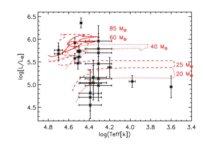
Figure 8: Luminosities of massive stars in the Cl 1813-178 cluster are plotted versus effective temperatures. Values are taken from Table 2. Stellar tracks for stars of 20, 25, 40, 60, and 85 M_⊙, based on rotating Geneva models with a solar metallicity, canonical mass-loss rates, and initial rotational velocity of 300 km s^-1 are also shown with dotted, dashed and continuous lines. For clarity, we use different line styles together with labels to indicate each model.

7 The cluster mass

By adding the masses of the spectroscopically identified massive stars, we estimated a minimum cluster mass of 990 M_⊙. We considered all 34 stars with $J-$K_s between 1 and 3 mag, and K_s$<10$ mag. By assuming that they all have masses greater than 35 M_⊙, and using a Salpeter mass function integrated from 0.8 to 120 M_⊙, we estimated a cluster mass of $13000\pm 3000$ M_⊙, where the error is the Poisson error of the number of massive stars. By assuming that these 34 stars have masses greater than 25 M_⊙, we obtained a cluster mass of $8700\pm 2000$ M_⊙. The two calculations take into account the uncertainties of the mass at the TO (25-35 M_⊙), predicted for a coeval population with an age of 4-4.5 Myr.

The Cl 1813-178 cluster is, therefore, a new addition to the list of 13 known young massive clusters ($\geq 10^{4}$ M_⊙) in the Milky Way (Messineo et al., 2009; Negueruela et al., 2010).

8 Cluster surroundings

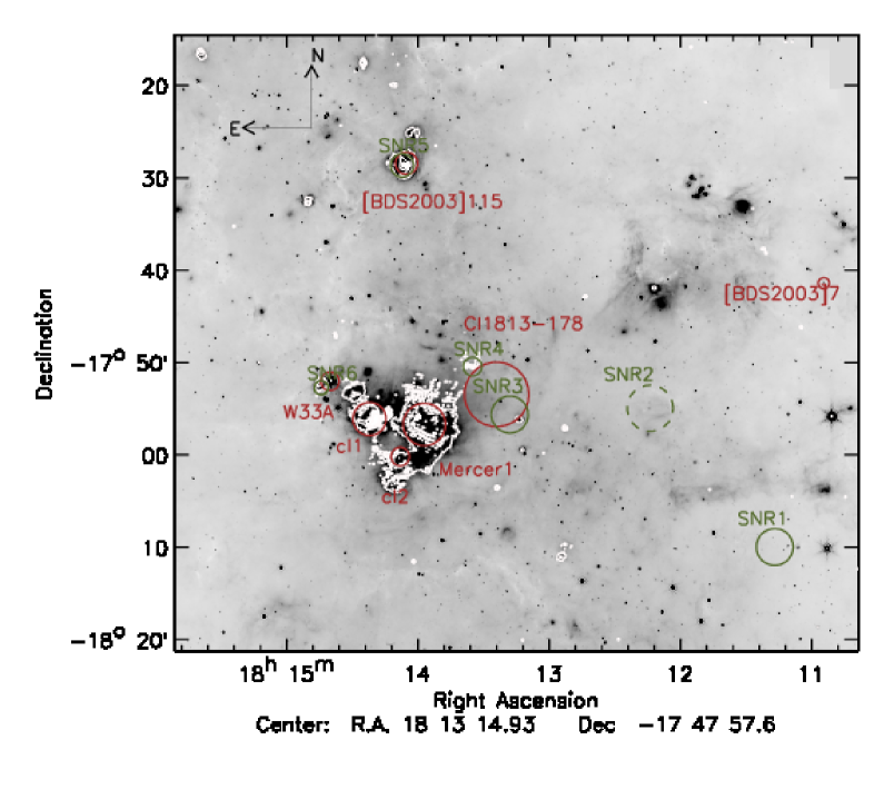
Figure 9: 24 $\mu$m emission from MIPSGAL (Carey et al., 2009) of the whole W33 complex. The white contours show 20 cm radio continuum emission from MAGPIS (White et al., 2005). Contour levels are 0.003, 0.009 and 0.020 mJy beam^-1; the beam size is 6.2^′′$\times$ 5.4^′′, FWHM, and the position angle of the major axis is along the north-south direction. Circles and labels indicate the location of the stellar clusters and candidate SNRs.

A 24 $\mu$m image from MIPSGAL, the survey of the inner Galactic plane using the Multiband Infrared Photometer for Spitzer aboard the Spitzer Space Telescope (Carey et al., 2009), of the whole W33 region is shown in Fig. 9, together with contours of radio continuum emission at 20 cm (White et al., 2005). The complex extends over an area of roughly 25^′$\times$20^′ (Bieging et al., 1978). Radio observations show that W33 is made up of a number of discrete sources. Some of these radio sources have been classified as candidate SNRs by Brogan et al. (2006) and Helfand et al. (2006) on the basis of morphology and spectral indexes, with MAGPIS data (White et al., 2005). See Table 6.

The Cl 1813-178 cluster appears located on the edge of the W33 complex. The radial velocity of the K2I star in the Cl 1813-178 cluster is of 62$\pm$4 km s^-1 (PaperI), and well agrees with the high-velocity gas component of W33. The spatial coincidence of the Cl 1813-178 cluster with the SNR G12.82-0.02 and G12.72-0.00 has already been reported in PaperI, and support the association of the cluster with the complex. The filamentary shape of the Cl 1813-178 stellar cluster and its location on the edge of W33 suggests a secondary episode of star formation, perhaps triggered by an expanding shell.

We searched for other possible candidate clusters and associations with SNRs in the direction of the W33 complex. A number of candidate stellar clusters have been identified in GLIMPSE and 2MASS images in the direction of the W33 region by Mercer et al. (2005) and Bica et al. (2003), which we list in Table 5. The W33 MYSO (Davies et al., 2010) is projected into SNR6 (G13.1875+0.0389) (Helfand et al., 2006). The spatial coincidence of the SNR and the MYSO suggests a physical association. The W33A MYSO could be an episode of triggered star formation induced by a supernova explosion. Mercer1 candidate cluster is the object number #1 in the list of Mercer et al. (2005). It was identified as a stellar overdensity in the GLIMPSE catalog with an automatic algorithm. It is located at the center of the molecular complex, and it appears as a spread overdensity. Two other candidates are reported in literature in the surrounding of the W33 complex, but without a clear connection with the W33 complex. The BDS2003-115 candidate cluster is about 20^′ North of the main W33 complex and is associated with SNR5 (G12.83-0.02) (Helfand et al., 2006). The BDS2003-7 candidate cluster appears as a small group of stars without associated radio emission (Bica et al., 2003).

We visually inspected the 2MASS images, and located two other clumps of stars (cl1 and cl2). The cl1 candidate appears as a group of point sources on bright nebular emission in the 2MASS K_s  image. Inspection of the GLIMPSE and MAGPIS images reveals the presence of an HII region, suggesting the presence of massive stars (see Table 5 and Figs. 10 and 11). The cl2 candidate is another small concentration of bright stars (K_s=8-10 mag) in another HII region. Nothing is reported in previous literature about both, cl1 and cl2, clumps. In addition, we searched for stellar over-densities in the direction of the W33 complex using both 2MASS and GLIMPSE star-counts. Detections are hampered by strong variations of the background level, which are due to variations of interstellar extinction and nebular emission. A spectroscopic and photometric follow-up study of these regions with SINFONI and UKIDSS data is ongoing, in order to confirm the presence of massive stars.

Near-infrared spectroscopic follow-up observations are needed to characterize these sources, and to confirm their association with the W33 complex. However, the associations of Cl 1813-178, cl1, and cl2 with HII regions and/or SNRs suggest that these are other condensation of massive stars in the W33 complex.

Table 5: List of candidate clusters in the direction of the W33 complex.

ID	RA	DEC	Radius(′)	References
Cl 1813-178	18 13 24	-17 53 31	3.5	PaperI
Mercer1	18 13 57	-17 56 46	2.3	(Mercer et al., 2005)
BDS2003-115	18 14 05	-17 28 29	1.2	(Bica et al., 2003)
BDS2003-7	18 10 55	-17 41 25	0.6	(Bica et al., 2003)
cl1	18 14 22	-17 56 10	1.8	Present work
cl2	18 14 08	-18 00 15	1.0	Present work

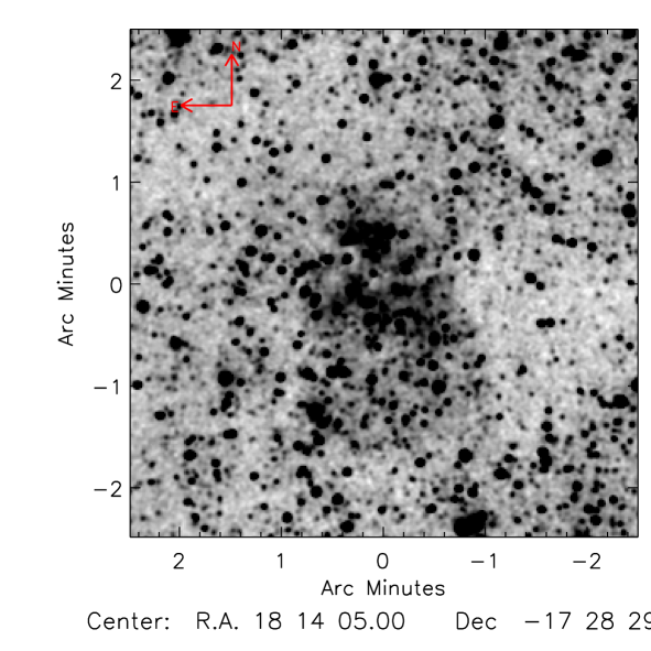
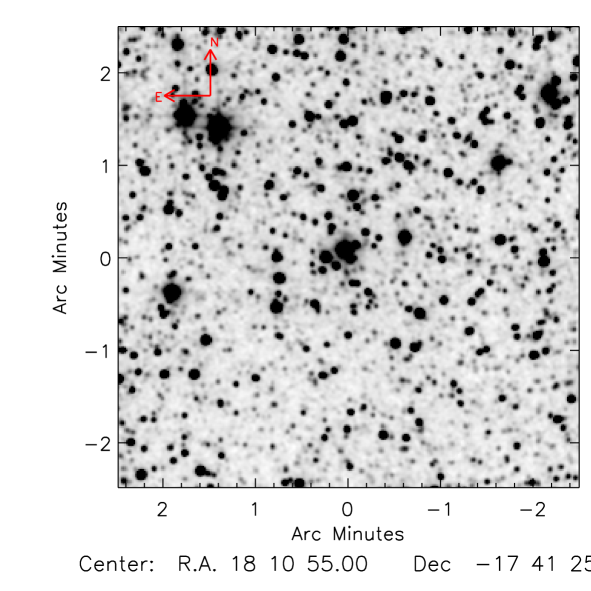
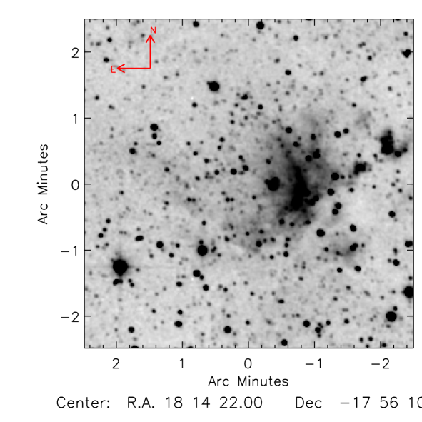
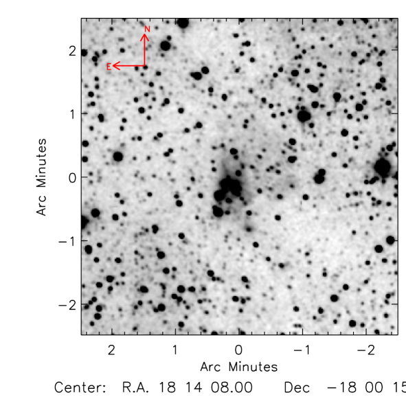
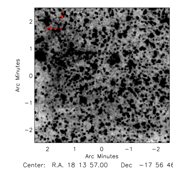
Figure 10: 2MASS K_s images of the BDS2003-115 cluster (top-left), the BDS2003-7 cluster (top-middle), the cl1 cluster (top-right), the cl2 cluster (bottom-left), and the Mercer1 cluster (bottom-middle).

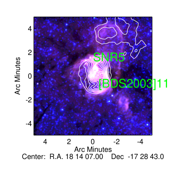
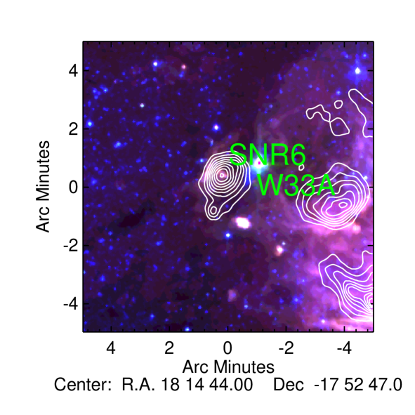
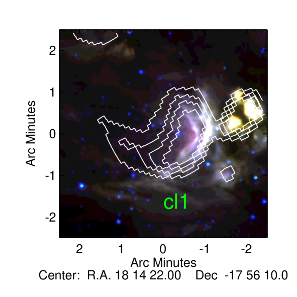
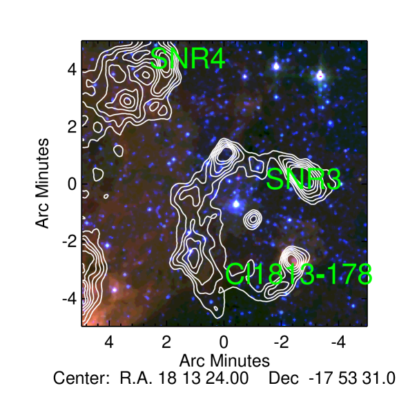
Figure 11: Composite images of SNR5, SNR6, cl1, cl2, and Cl 1813-178. In blue the GLIMPSE 3.6 $\mu$m, in green the 5.8$\mu$m, and in red the 8.0$\mu$m. Over-plotted are contours of 90 cm radio continuum emission detected by MAGPIS (White et al., 2005).

Table 6: List of candidate SNRs

ID	Name	RA	DEC	Radius(′)	References
SNR1	G12.26+0.30	18:11:17	-18:10:00	4	(Brogan et al., 2006; Helfand et al., 2006)
SNR2	G12.58+0.22 ?	18:12:14	-17:55:00	5	(Brogan et al., 2006)
SNR3	G12.72-0.00	18:13:18	-17:55:42	4	(Brogan et al., 2006; Helfand et al., 2006)
SNR4	G12.83-0.02	18:13:35	-17:50:30	2	(Brogan et al., 2006; Helfand et al., 2006)
SNR5	G13.1875+0.0389	18:14:07	-17:28:43	2.5	(Helfand et al., 2006)
SNR6	G12.9139-0.2806	18:14:44	-17:52:47	1.5	(Helfand et al., 2006)

9 Summary

A near-infrared spectroscopic survey of the brightest stars in the direction of the Cl 1813-178 cluster is presented. Among the 61 observed stars, 25 massive stars were detected. Two WR stars of type WN7, a cLBV, and 21 OB stars were identified. Among the OB stars, a O8-O9If star and a O6-O7If star were discovered. Eight of these evolved stars also have X–ray emission, as detected by the Chandra and XMM satellites. The hardness of the X–ray emission from the two WN7 stars strongly suggests binary systems.

A spectro-photometric analysis of the OB stars reveals 14 supergiants, 4 giants, and 3 dwarfs. From the giants, dwarfs and WRs, we derived average spectrophotometric distances of $3.8\pm 1.0$ kpc, and $2.9\pm 0.8$ kpc, and $4.2\pm 1.6$ kpc. The distances from giants and WRs is in agreement with the kinematic distance. The distance estimates from dwarfs are only consistent with the kinematic distance if the dwarfs are late O stars.

The mixture of evolved massive stars is reminiscent of other Galactic young massive clusters, such as Westerlund 1, Quintuplet, Galactic center, and Cl 1806-20. We estimated stellar luminosities, therefore, masses by comparing the luminosities with evolutionary tracks from the Geneva group. By assuming a Salpeter mass function, we obtained a cluster mass of $1.0\pm 0.2\times 10^{4}$ M_⊙. A likely cluster age of 4-4.5 Myr is derived, however, a spread in age of about 1 Myr cannot be excluded. In order to better constrain the degree of coevality, further spectroscopic observations are required.

The Cl 1813-178 cluster is located on the Western edge of the W33 complex. We have located several other candidate stellar clusters that could belong to the same complex.

Appendix A Late-type stars

The EW(CO)s can be used for classification in subclasses of late-type stars. There is a linear correlation between stellar effective temperatures and EW(CO)s of the CO bands. Furthermore, since giants and supergiants follow two different relations, information on the luminosity class can also be obtained (see e.g. Figer et al., 2006; Davies et al., 2007).

Among the observed 60 stars, 37 are found to be late-type stars. For 36 of them, spectra were taken with the K-long grism, covering the region of the CO band-head at 2.29 $\mu$m. CO bands at 2.29 $\mu$m in absorption are detected in all spectra. Star #55 was observed only with the K-short grism; however, the presence of Na lines (at 2.2075 and 2.2077 $\mu$m) and Mg I at 2.11 $\mu$m suggests a spectral type later than G0.

The equivalent widths of 32 of these late-type stars are compatible with that of giant stars with spectral type from K0III to M7III (Table 7). For star #58 we do not report any spectral type, since its spectrum has a poor signal to noise.

Star #32, #38, and #39 have EW(CO)s typical of RSG stars, with spectral types M2.5, M3.5 and M1, respectively. However, their photometric properties indicate that they are unrelated to the stellar cluster. Star #1 is consistent with being a K2-K5I cluster member (see PaperI).

Young massive clusters with ages from 4 to 30 Myrs may contain yellow supergiants (YSG) stars, e.g. the Westerlund 1 (Clark et al., 2005) and RSGC1 clusters (Figer et al., 2006). YSG are rare F or G-type supergiants in transition towards the RSG phase or, back from the RSG locus, evolving blue-ward. In a coeval population, YSGs or RSGs are expected to be brighter in K_s than early-type massive stars. In the Cl 1813-178 cluster, all detected stars with CO band-head at 2.29 $\mu$m appear fainter than the brightest OB stars, and the gap between the brightest early-type star (K_s=6.75 mag) and the K2I star (K_s=3.79 mag) is devoid of stars. Furthermore, the CO band-heads of the five late-type stars with K_s between 7 and 8 mag indicate late M giants (M2-M5), or late K supergiants (K2-K4). Their EW(CO)s are not consistent with being F or G supergiants.

Table 7: List of field stars spectroscopically observed.

ID	Ra	Dec	B	V	R	J	H	Ks	[3.6]	[4.5]	[5.8]	[8.0]	tel.	Sp
10	18 13 47.56	-17 57 01.43	15.32	$\cdots$	13.64	10.76	9.89	9.60	9.31	9.34	9.22	9.20	ukirt	K0.5III
27	18 13 14.39	-17 54 47.87	$\cdots$	$\cdots$	17.48	9.50	7.84	7.08	6.90	6.81	6.55	6.54	ukirt-keck	M4.5III
28	18 13 35.03	-17 54 26.11	12.85	12.70	$\cdots$	8.53	7.53	7.21	7.16	7.22	7.00	7.03	keck	M4III
29	18 13 29.14	-17 52 27.18	16.19	13.16	13.13	9.00	7.94	7.50	7.26	7.51	7.26	7.28	keck	M3III
30	18 13 26.87	-17 55 27.50	$\cdots$	$\cdots$	$\cdots$	10.35	8.40	7.52	7.07	7.12	6.90	6.87	keck	M5III
31	18 13 16.80	-17 55 40.02	21.42	16.78	14.36	9.79	8.47	7.93	7.63	7.72	7.58	7.55	keck	M2.5III
32	18 13 16.35	-17 50 29.89	$\cdots$	$\cdots$	$\cdots$	13.53	9.85	8.08	6.82	6.80	6.41	6.47	keck	M2.5I
33	18 13 25.93	-17 57 39.84	16.25	16.37	$\cdots$	11.61	9.27	8.24	7.55	7.66	7.39	7.41	keck	M5.5III
34	18 13 28.59	-17 50 30.78	12.42	11.65	11.15	9.10	8.51	8.40	8.34	8.40	8.31	8.27	keck	K0.5III
35	18 13 34.10	-17 51 28.59	$\cdots$	$\cdots$	$\cdots$	11.55	9.40	8.49	7.78	7.92	7.64	7.66	keck	M2III
36	18 13 31.44	-17 52 41.01	$\cdots$	$\cdots$	$\cdots$	14.13	10.40	8.50	7.00	6.83	6.35	6.43	ukirt-keck	M7III
37	18 13 21.37	-17 58 04.63	15.18	13.87	14.64	9.79	8.81	8.51	8.36	8.46	8.28	8.19	keck	K3.5III
38	18 13 28.96	-17 55 52.85	$\cdots$	$\cdots$	$\cdots$	17.08	11.22	8.54	6.89	6.19	5.63	5.41	keck	M3.5I
39	18 13 29.36	-17 51 47.65	$\cdots$	$\cdots$	$\cdots$	13.83	10.34	8.61	7.50	7.49	7.08	7.18	ukirt	M1I
40	18 13 14.67	-17 51 32.41	16.43	14.40	13.69	10.08	9.06	8.69	8.45	8.53	8.39	8.37	ukirt	K5.5III
41	18 13 12.16	-17 51 58.47	$\cdots$	$\cdots$	$\cdots$	11.60	9.63	8.78	8.17	8.24	8.04	8.03	ukirt	K5III
42	18 13 19.97	-17 53 42.39	$\cdots$	$\cdots$	$\cdots$	13.94	10.46	8.80	7.68	7.68	7.33	7.44	ukirt	M6III
43	18 13 21.98	-17 53 20.70	$\cdots$	$\cdots$	$\cdots$	13.25	10.17	8.84	7.83	7.82	7.46	7.35	ukirt	M3III
44	18 13 14.87	-17 57 21.60	18.60	$\cdots$	18.54	14.39	10.65	8.86	7.58	7.56	7.18	7.27	ukirt	M7III
45	18 13 19.55	-17 55 01.00	17.16	17.08	$\cdots$	13.19	10.30	8.96	8.05	8.05	7.76	7.82	ukirt	M2.5III
46	18 13 25.70	-17 52 01.02	$\cdots$	$\cdots$	$\cdots$	13.60	10.45	8.99	7.97	7.95	7.63	7.66	ukirt	M6.5III
47	18 13 12.25	-17 51 26.83	$\cdots$	$\cdots$	$\cdots$	13.14	10.36	9.06	8.22	8.31	7.92	8.03	ukirt	M6III
48	18 13 17.58	-17 54 52.09	$\cdots$	$\cdots$	$\cdots$	14.00	10.63	9.07	7.91	7.99	7.66	7.68	ukirt	M7III
49	18 13 25.18	-17 49 35.98	13.82	13.12	12.08	10.14	9.38	9.12	9.02	9.18	9.00	9.03	ukirt	K3III
50	18 13 10.77	-17 54 47.58	$\cdots$	$\cdots$	$\cdots$	11.51	9.83	9.13	8.74	8.77	8.56	8.62	ukirt	K5.5III
51	18 13 18.55	-17 56 18.30	$\cdots$	$\cdots$	18.42	11.17	9.73	9.16	8.78	8.84	8.67	8.68	ukirt	K4III
52	18 13 35.17	-17 50 44.06	$\cdots$	$\cdots$	$\cdots$	13.90	10.68	9.19	8.15	8.10	7.78	7.92	ukirt	M2.5III
53	18 13 38.15	-17 57 07.51	$\cdots$	$\cdots$	$\cdots$	15.51	11.31	9.26	7.95	7.90	7.40	7.67	ukirt	M6.5III
54	18 13 35.19	-17 57 33.25	12.71	12.33	11.85	10.00	9.46	9.30	9.28	9.31	9.19	9.21	ukirt	K0III
55	18 13 27.03	-17 50 27.76	15.43	14.38	15.62	10.64	9.66	9.38	9.23	9.22	9.25	9.17	ukirt	$>$G
56	18 13 18.70	-17 51 14.93	20.67	15.81	16.69	10.90	9.76	9.40	9.21	9.25	9.19	9.24	ukirt	K5.5III
57	18 13 17.23	-17 55 21.81	15.93	13.67	15.02	10.61	9.83	9.56	9.36	9.45	9.33	9.23	ukirt	K0.5III
58	18 13 12.99	-17 54 02.32	$\cdots$	$\cdots$	$\cdots$	14.55	11.42	10.02	9.06	9.01	8.71	8.75	ukirt	$>G$
59	18 13 20.01	-17 53 50.13	15.83	14.87	15.93	11.54	10.73	10.52	10.32	10.42	10.34	10.15	ukirt	K1.5III
60	18 13 20.65	-17 53 50.28	$\cdots$	$\cdots$	$\cdots$	16.06	12.65	10.58	10.04	9.97	9.70	9.70	ukirt	M6.5III
61	18 13 26.31	-17 53 57.05	$\cdots$	17.34	$\cdots$	14.99	13.30	11.77	10.73	10.62	10.35	10.48	ukirt	K4.5III

Note. — For each star, number designations and coordinates (J2000) are followed by magnitudes measured in different bands. J,H, and K_s measurements are from 2MASS, while the magnitudes at 3.6 $\mu$m, 4.5 $\mu$m, 5.8 $\mu$m, and 8 $\mu$m are from GLIMPSE. $B$, $V$, and $R$ associations are taken from the astrometric catalog NOMAD.

Appendix B Effective temperatures and bolometric corrections

In order to estimate stellar luminosities, estimates of effective temperatures and bolometric corrections as a function of spectral type need to be known. Since an homogeneous calibration extending from O stars down to early A stars is missing, we summarize all the adopted values.

For O-type stars, we used the T_eff from Martins et al. (2005). For early B supergiants, we adopted the T_eff values given by Crowther et al. (2006b), while, for late B and A supergiants, those by Humphreys & McElroy (1984). For B giants, we adopted the T_eff by Humphreys & McElroy (1984). For B and A dwarfs, we used T_eff estimated by Humphreys & McElroy (1984) and Johnson (1966).

For O-type stars, we used the bolometric corrections in K-band (BC_K) by Martins & Plez (2006). For early B-type stars, we used those provided by Bibby et al. (2008). We estimated the BC_Ks of late B supergiants and giants by assuming bolometric corrections in the V-band (BC_V) from Humphreys & McElroy (1984), and intrinsic $V-K$ colors from Koornneef (1983) and Wegner (1994). For dwarf stars, a set of homogeneous BC_K was obtained by interpolating an isochrone of 0.5 Myr and solar metallicity from Lejeune & Schaerer (2001) at the assumed effective temperatures (Humphreys & McElroy, 1984; Johnson, 1966).

Table 8: Infrared colors and BC_K of supergiant stars.

Sp.	Teff	BCK	$J-K$	$H-K$	Reference
O3	42551	$-$4.69	$-$0.21	$-$0.10	Martins et al. (2005),Martins & Plez (2006)
O4	40702	$-$4.55	$-$0.21	$-$0.10	Martins et al. (2005),Martins & Plez (2006)
O5	38520	$-$4.40	$-$0.21	$-$0.10	Martins et al. (2005),Martins & Plez (2006)
O6	35747	$-$4.25	$-$0.21	$-$0.10	Martins et al. (2005),Martins & Plez (2006)
O7	33326	$-$4.09	$-$0.21	$-$0.10	Martins et al. (2005),Martins & Plez (2006)
O8	31009	$-$3.93	$-$0.21	$-$0.10	Martins et al. (2005),Martins & Plez (2006)
O9	29569	$-$3.75	$-$0.21	$-$0.10	Martins et al. (2005),Martins & Plez (2006)
B0	27500	$-$3.30	$-$0.11	$-$0.04	Crowther et al. (2006a), Bibby et al. (2008)
B1	21500	$-$2.65	$-$0.09	$-$0.03	Crowther et al. (2006a), Bibby et al. (2008)
B2	18500	$-$2.10	$-$0.07	$-$0.03	Crowther et al. (2006a), Bibby et al. (2008)
B3	15500	$-$1.70	$-$0.04	$-$0.03	Crowther et al. (2006a), Bibby et al. (2008)
B5	13700	$-$0.95	0.00	$-$0.01	Humphreys & McElroy (1984),(Koornneef, 1983)
B8	10900	$-$0.47	0.05	0.00	Humphreys & McElroy (1984),(Koornneef, 1983)
B9	10250	$-$0.27	0.07	0.01	Humphreys & McElroy (1984),(Koornneef, 1983)
A0	9500	$-$0.09	0.09	0.01	Humphreys & McElroy (1984),(Koornneef, 1983)
A2	9100	0.14	0.11	0.02	Humphreys & McElroy (1984),(Koornneef, 1983)
A5	8500	0.36	0.12	0.02	Humphreys & McElroy (1984),(Koornneef, 1983)

Table 9: Infrared colors and BC_K of giant stars.

Sp.	Teff	BCK	$J-K$	$H-K$	Reference
O3	42942	$-4.85$	$-0.21$	$-0.10$	Martins et al. (2005),Martins & Plez (2006)
O4	41486	$-4.70$	$-0.21$	$-0.10$	Martins et al. (2005),Martins & Plez (2006)
O5	39507	$-4.54$	$-0.21$	$-0.10$	Martins et al. (2005),Martins & Plez (2006)
O6	36673	$-4.37$	$-0.21$	$-0.10$	Martins et al. (2005),Martins & Plez (2006)
O7	34638	$-4.19$	$-0.21$	$-0.10$	Martins et al. (2005),Martins & Plez (2006)
O8	32573	$-4.00$	$-0.21$	$-0.10$	Martins et al. (2005),Martins & Plez (2006)
O9	30737	$-3.80$	$-0.21$	$-0.10$	Martins et al. (2005),Martins & Plez (2006)
B0	30300	$-3.59$	$-0.18$	$-0.09$	Humphreys & McElroy (1984),(Wegner, 1994)
B1	21100	$-2.65$	$-0.19$	$-0.10$	Humphreys & McElroy (1984),(Wegner, 1994)
B2	18000	$-2.16$	$-0.18$	$-0.10$	Humphreys & McElroy (1984),(Wegner, 1994)
B3	17100	$-1.96$	$-0.12$	$-0.06$	Humphreys & McElroy (1984),(Wegner, 1994)
B5	16300	$-1.81$	$-0.10$	$-0.06$	Humphreys & McElroy (1984),(Wegner, 1994)
B8	12550	$-0.94$	$-0.03$	$-0.02$	Humphreys & McElroy (1984),(Wegner, 1994)
B9	11400	$-0.55$	$-0.02$	$-0.01$	Humphreys & McElroy (1984),(Wegner, 1994)

Table 10: Infrared colors and BC_K of dwarf stars.

Sp.	Teff	BCK	$J-K$	$H-K$	Reference
O3	44616	$-4.76$	$-0.19$	$-0.04$	Martins et al. (2005),Lejeune & Schaerer (2001)
O4	43419	$-4.70$	$-0.19$	$-0.04$	Martins et al. (2005),Lejeune & Schaerer (2001)
O5	41540	$-4.62$	$-0.18$	$-0.04$	Martins et al. (2005),Lejeune & Schaerer (2001)
O6	38151	$-4.39$	$-0.17$	$-0.04$	Martins et al. (2005),Lejeune & Schaerer (2001)
O7	35531	$-4.15$	$-0.17$	$-0.04$	Martins et al. (2005),Lejeune & Schaerer (2001)
O8	33383	$-3.98$	$-0.16$	$-0.04$	Martins et al. (2005),Lejeune & Schaerer (2001)
O9	31524	$-3.86$	$-0.15$	$-0.04$	Martins et al. (2005),Lejeune & Schaerer (2001)
B0	29600	$-3.72$	$-0.15$	$-0.04$	Humphreys & McElroy (1984),Lejeune & Schaerer (2001)
B1	24150	$-3.21$	$-0.13$	$-0.03$	Humphreys & McElroy (1984),Lejeune & Schaerer (2001)
B2	19700	$-2.60$	$-0.12$	$-0.03$	Humphreys & McElroy (1984),Lejeune & Schaerer (2001)
B3	18700	$-2.46$	$-0.11$	$-0.02$	Humphreys & McElroy (1984),Lejeune & Schaerer (2001)
B5	13800	$-1.43$	$-0.06$	$-0.01$	Johnson (1966),Lejeune & Schaerer (2001)
B8	12200	$-1.00$	$-0.03$	$-0.00$	Johnson (1966),Lejeune & Schaerer (2001)
B9	10600	$-0.52$	$-0.00$	$0.00$	Johnson (1966),Lejeune & Schaerer (2001)
A0	9850	$-0.25$	$0.02$	$0.01$	Johnson (1966),Lejeune & Schaerer (2001)
A2	9120	$-0.03$	$0.04$	$0.02$	Johnson (1966),Lejeune & Schaerer (2001)
A5	8260	$0.28$	$0.08$	$0.03$	Johnson (1966),Lejeune & Schaerer (2001)

Table 11: Infrared colors and BC_K adopted for RSGs and WRs.

Sp.	Teff	BCK	$J-K$	$H-K$	Reference
K2I	4015	$+2.5$	$+0.65$	$+0.13$	Levesque et al. (2005),Koornneef (1983)
M1I	3745	$+2.7$	$+1.00$	$+0.22$	Levesque et al. (2005),Koornneef (1983)
M2.5I	3615	$+2.8$	$+1.06$	$+0.27$	Levesque et al. (2005),Koornneef (1983)
M3.5I	3550	$+2.9$	$+1.16$	$+0.28$	Levesque et al. (2005),Koornneef (1983)
WN7o		$-3.9$	$+0.13$	$+0.11$	Crowther et al. (2006a)
WN7b		$-3.5$	$+0.37$	$+0.27$	Crowther et al. (2006a)

References

- Benjamin et al. (2003) Benjamin, R. A., Churchwell, E., Babler, B. L., et al. 2003, PASP, 115, 953
- Beuther et al. (2007) Beuther, H., Churchwell, E. B., McKee, C. F., & Tan, J. C. 2007, Protostars and Planets V, 165
- Bibby et al. (2008) Bibby, J. L., Crowther, P. A., Furness, J. P., & Clark, J. S. 2008, MNRAS, 386, L23
- Bica et al. (2003) Bica, E., Dutra, C. M., Soares, J., & Barbuy, B. 2003, A&A, 404, 223
- Bieging et al. (1978) Bieging, J. H., Pankonin, V., & Smith, L. F. 1978, A&A, 64, 341
- Bonanos (2007) Bonanos, A. Z. 2007, ApJ, 133, 2696
- Brogan et al. (2006) Brogan, C. L., Gelfand, J. D., Gaensler, B. M., Kassim, N. E., & Lazio, T. J. W. 2006, ApJ, 639, L25
- Carey et al. (2009) Carey, S. J., Noriega-Crespo, A., Mizuno, D. R., et al. 2009, PASP, 121, 76
- Clark et al. (2009) Clark, J. S., Davies, B., Najarro, F., et al. 2009, A&A, 504, 429
- Clark et al. (2005) Clark, J. S., Larionov, V. M., & Arkharov, A. 2005, A&A, 435, 239
- Clark et al. (2008) Clark, J. S., Muno, M. P., Negueruela, I., et al. 2008, A&A, 477, 147
- Cohen (1996) Cohen, D. H. 1996, PASP, 108, 1140
- Comeron (2004) Comerón, F., Torra, J., Chiappini, C., et al. 2004, A&A, 425, 489
- Conti (1984) Conti, P. S. 1984, in IAU Symposium, Vol. 105, Observational Tests of the Stellar Evolution Theory, ed. A. Maeder & A. Renzini, 233–+
- Conti et al. (1995) Conti, P. S., Hanson, M. M., Morris, P. W., Willis, A. J., & Fossey, S. J. 1995, ApJ, 445, L35
- Crowther et al. (2006a) Crowther, P. A., Hadfield, L. J., Clark, J. S., Negueruela, I., & Vacca, W. D. 2006a, MNRAS, 372, 1407
- Crowther et al. (2006b) Crowther, P. A., Lennon, D. J., & Walborn, N. R. 2006b, A&A, 446, 279
- Dame et al. (2001) Dame, T. M., Hartmann, D., & Thaddeus, P. 2001, ApJ, 547, 792
- Davies et al. (2007) Davies, B., Figer, D. F., Kudritzki, R., et al. 2007, ApJ, 671, 781
- Davies et al. (2010) Davies, B., Lumsden, S. L., Hoare, M. G., Oudmaijer, R. D., & de Wit, W. 2010, MNRAS, 402, 1504
- Eldridge et al. (2008) Eldridge, J. J., Izzard, R. G., & Tout, C. A. 2008, MNRAS, 384, 1109
- Figer et al. (2006) Figer, D. F., MacKenty, J. W., Robberto, M., et al. 2006, ApJ, 643, 1166
- Figer et al. (1997) Figer, D. F., McLean, I. S., & Najarro, F. 1997, ApJ, 486, 420
- Funk et al. (2007) Funk, S., Hinton, J. A., Moriguchi, Y., et al. 2007, A&A, 470, 249
- Goss et al. (1978) Goss, W. M., Matthews, H. E., & Winnberg, A. 1978, A&A, 65, 307
- Hadfield et al. (2007) Hadfield, L. J., van Dyk, S. D., Morris, P. W., et al. 2007, MNRAS, 376, 248
- Hanson et al. (1996) Hanson, M. M., Conti, P. S., & Rieke, M. J. 1996, ApJS, 107, 281
- Hanson et al. (2005) Hanson, M. M., Kudritzki, R.-P., Kenworthy, M. A., Puls, J., & Tokunaga, A. T. 2005, ApJS, 161, 154
- Helfand et al. (2006) Helfand, D. J., Becker, R. H., White, R. L., Fallon, A., & Tuttle, S. 2006, AJ, 131, 2525
- Helfand et al. (2007) Helfand, D. J., Gotthelf, E. V., Halpern, J. P., et al. 2007, ApJ, 665, 1297
- Hillier & Miller (1998) Hillier, D. J. & Miller, D. L. 1998, ApJ, 496, 407
- Humphreys & McElroy (1984) Humphreys, R. M. & McElroy, D. B. 1984, ApJ, 284, 565
- Indebetouw et al. (2005) Indebetouw, R., Mathis, J. S., Babler, B. L., et al. 2005, ApJ, 619, 931
- Johnson (1966) Johnson, H. L. 1966, ARA&A, 4, 193
- Kleinmann & Hall (1986) Kleinmann, S. G. & Hall, D. N. B. 1986, ApJS, 62, 501
- Koornneef (1983) Koornneef, J. 1983, A&A, 128, 84
- Lejeune & Schaerer (2001) Lejeune, T. & Schaerer, D. 2001, A&A, 366, 538
- Levesque et al. (2005) Levesque, E. M., Massey, P., Olsen, K. A. G., et al. 2005, ApJ, 628, 973
- Lucy & White (1980) Lucy, L. B. & White, R. L. 1980, ApJ, 241, 300
- Martins et al. (2007) Martins, F., Genzel, R., Hillier, D. J., et al. 2007, A&A, 468, 233
- Martins & Plez (2006) Martins, F. & Plez, B. 2006, A&A, 457, 637
- Martins et al. (2005) Martins, F., Schaerer, D., & Hillier, D. J. 2005, A&A, 436, 1049
- Massey et al. (2001) Massey, P., DeGioia-Eastwood, K., & Waterhouse, E. 2001, AJ, 121, 1050
- Mauerhan et al. (2010) Mauerhan, J. C., Morris, M. R. , Cotera, A. , et al. 2010, ApJ, 713, 33
- Mercer et al. (2005) Mercer, E. P., Clemens, D. P., Meade, M. R., et al. 2005, ApJ, 635, 560
- Messineo et al. (2009) Messineo, M., Davies, B., Ivanov, V. D., et al. 2009, ApJ, 697, 701
- Messineo et al. (2008) Messineo, M., Figer, D. F., Davies, B., et al. 2008, ApJ, 683, L155
- Messineo et al. (2005) Messineo, M., Habing, H. J., Menten, K. M., et al. 2005, A&A, 435, 575
- Messineo et al. (2004) Messineo, M., Habing, H. J., Menten, K. M., et al. 2004, A&A, 418, 103
- Messineo (2004) Messineo, M. 2004, Ph.D. Thesis [arXiv:astro-ph/0407559]
- Meynet & Maeder (2000) Meynet, G. & Maeder, A. 2000, A&A, 361, 101
- Meynet & Maeder (2003) Meynet, G. & Maeder, A. 2003, A&A, 404, 975
- Meynet et al. (1994) Meynet, G., Maeder, A., Schaller, G., Schaerer, D., & Charbonnel, C. 1994, A&AS, 103, 97
- Moorwood et al. (1998) Moorwood, A., Cuby, J., & Lidman, C. 1998, The Messenger, 91, 9
- Morris et al. (1996) Morris, P. W., Eenens, P. R. J., Hanson, M. M., Conti, P. S., & Blum, R. D. 1996, ApJ, 470, 597
- Najarro (2001) Najarro, F. 2001, in Astronomical Society of the Pacific Conference Series, Vol. 233, P Cygni 2000: 400 Years of Progress, ed. M. de Groot & C. Sterken, 133–+
- Najarro et al. (1999) Najarro, F., Hillie, D. J., Kudritzki, R. P., & Morris, P. W. 1999, in ESA Special Publication, Vol. 427, The Universe as Seen by ISO, ed. P. Cox & M. Kessler, 377–+
- Negueruela et al. (2010) Negueruela, I., González-Fernández, C., Marco, A., Clark, J. S., & Martínez-Núñez, S. 2010, A&A, 513, A74+
- Nota et al. (1995) Nota, A., Livio, M., Clampin, M., & Schulte-Ladbeck, R. 1995, ApJ, 448, 788
- Panagia (1973) Panagia, N. 1973, AJ, 78, 929
- Pollock (1987) Pollock, A. M. T. 1987, ApJ, 320, 283
- Reid et al. (2009) Reid, M. J., Menten, K. M., Zheng, X. W., et al. 2009, ApJ, 700, 137
- Ritchie (2009) Ritchie, B. W., Clark, J. S., Negueruela, I. , & Najarro, F. 2009, ApJ, 507, 1597
- Schaerer et al. (1993) Schaerer, D., Meynet, G., Maeder, A., & Schaller, G. 1993, A&AS, 98, 523
- Schaller et al. (1992) Schaller, G., Schaerer, D., Meynet, G., & Maeder, A. 1992, A&AS, 96, 269
- Skinner et al. (2010) Skinner, S. L., Zhekov, S. A., Güdel, M., Schmutz, W., & Sokal, K. R. 2010, AJ, 139, 825
- Skrutskie et al. (2006) Skrutskie, M. F., Cutri, R. M., Stiening, R., et al. 2006, AJ, 131, 1163
- Waldron & Cassinelli (2007) Waldron, W. L. & Cassinelli, J. P. 2007, ApJ, 668, 456
- Wallace & Hinkle (1996) Wallace, L. & Hinkle, K. 1996, ApJS, 107, 312
- Wegner (1994) Wegner, W. 1994, MNRAS, 270, 229
- White et al. (2005) White, R. L., Becker, R. H., & Helfand, D. J. 2005, AJ, 130, 586
- Woosley & Bloom (2006) Woosley, S. E. & Bloom, J. S. 2006, ARA&A, 44, 507
- Zacharias et al. (2004) Zacharias, N., Monet, D. G., Levine, S. E., et al. 2004, in Bulletin of the American Astronomical Society, Vol. 36, Bulletin of the American Astronomical Society, 1418