Evolutionary tracks of tidally stirred disky dwarf galaxies

Abstract

Using collisionless $N$-body simulations, we investigate the tidal evolution of late-type, rotationally supported dwarfs inside Milky Way-sized host galaxies. Our study focuses on a wide variety of dwarf orbital configurations and initial structures. During the evolution, the disky dwarfs undergo strong mass loss, the stellar disks are transformed into spheroids, and rotation is replaced by random motions of the stars. Thus, the late-type progenitors are transformed into early-type dwarfs as envisioned by the tidal stirring model for the formation of dwarf spheroidal (dSph) galaxies in the Local Group. We determine the photometric properties of the dwarfs, including the total visual magnitude, the half-light radius and the central surface brightness as they would be measured by an observer near the galactic center. Special emphasis is also placed on studying their kinematics and shapes. We demonstrate that the measured values are biased by a number of observational effects including the increasing angle of the observation cone near the orbital pericenter, the fact that away from the pericenter the tidal tails are typically oriented along the line of sight, and the fact that for most of the evolution the stellar components of the dwarfs are triaxial ellipsoids whose major axis tumbles with respect to the line of sight. Finally, we compare the measured properties of the simulated dwarfs to those of dwarf galaxies in the Local Group. The evolutionary tracks of the dwarfs in different parameter planes and the correlations between their different properties, especially the total magnitude and the surface brightness, strongly suggest that present-day dSph galaxies may have indeed formed from late-type progenitors as proposed by the tidal stirring scenario.

1. Introduction

The population of dwarf galaxies of the Local Group (for a review see Mateo 1998; Tolstoy et al. 2009) can be divided into two rather distinct subgroups, the dwarf irregular (dIrr) galaxies occupying larger distances from the big galaxies, the Milky Way and Andromeda, and dwarf spheroidal (dSph) objects clustering near their respective hosts. While the former are typically disky, bright, dominated by rotation, gas-rich and still forming stars, the latter are rounder, faint, supported mainly by random motions, gas-poor and dominated by old stellar populations.

The dIrr galaxies are believed to be of primordial origin, i.e. formed by gas accretion onto potential wells of small dark matter halos. The formation of dSph galaxies, on the other hand, probably required some evolution that may occur either in isolation by purely baryonic processes such as cooling, star formation, feedback from supernovae and UV background radiation (Ricotti & Gnedin 2005; Tassis et al. 2008; Sawala et al. 2010) or be induced by gravitational interactions with the environment in the form of galaxy harassment (e.g., Moore et al. 1996) resonant stripping (D’Onghia et al. 2009) or tidal stirring (Mayer et al. 2001a,b; Kazantzidis et al. 2004).

The tidal stirring scenario proposed by Mayer et al. (2001a,b) is particularly promising as it provides a link between the two types of dwarf galaxies observed in the Local Group. It postulates that dIrrs were actually progenitors of dSph galaxies and provides a mechanism for such transformation in the form of tidal stripping and tidal shocking of the dwarfs on orbits around the hosts. As the efficiency of these mechanisms increases with the decreasing distance of the dwarf galaxy from its host, it also naturally explains the morphology-distance relation observed in the Local Group. When combined with ram pressure stripping and the effect of the UV background (Bullock et al. 2000; Susa & Umemura 2004) the model can also account for the low gas content and the very high mass-to-light ratios of some dwarfs (Mayer et al. 2006, 2007; see also Mayer 2010 for a review).

The efficiency of the tidal transformation of disky dwarfs into dSph galaxies has been recently explored in great detail by Kazantzidis et al. (2011, hereafter K11) for different orbital and structural configurations of the dwarfs interacting with the Milky Way. The dwarfs were initially composed of a stellar disk embedded in a more extended dark matter halo. They confirmed the general picture sketched earlier by Mayer et al. (2001a,b) and Klimentowski et al. (2009a): in most cases the tidal interaction of the dwarf with the Milky Way results in strong mass loss, the morphological transformation of the disk to a bar and then a spheroid and the transition from ordered (rotation) to random motion of the stars. Only in three out of 19 simulated cases (where the orbits were very extended or the dwarf’s halo very concentrated) did the end product retain enough of its initial disky characteristics that it could not be classified as a dSph galaxy. Similarly, in almost all cases, the morphological transformation involved the formation at the first pericenter passage of a tidally induced bar that was shortened in the subsequent evolution.

The study of K11 focused on the intrinsic properties of the dwarfs which are best suited to describe their dynamics as precisely as possible, but can only be measured accurately in the idealized situation of $N$-body simulations where full 3D information is available. Here, we focus on strictly observational parameters that can be directly compared to real data. The purpose of the present work is therefore two-fold. First, we will measure the observational parameters of the dwarfs in a realistic way and identify possible biases affecting the measurements in the environment characteristic for dwarf galaxies in the Local Group. Second, we will explore the correlations between the observed parameters of the dwarfs in order to see if these can provide some insight into their formation scenarios.

The paper is organized as follows. In section 2 we briefly describe the simulations used in this work. Section 3 discusses the way we measure the observational parameters focusing on different observational biases that affect them. We also describe their variability on different timescales and its origin. In section 4 we present long-term evolution of the measured parameters for different orbits and different initial structure of the dwarfs. In section 5 we compare our results to observations. The discussion follows in the last section.

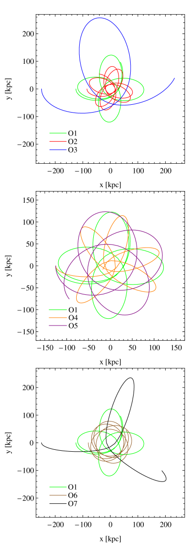
Figure 1.— Orbits of the dwarf galaxy in simulations O1-O7. In all panels we repeat the orbit O1 for reference. In the upper panel all three orbits have the same eccentricity $r_{\rm apo}/r_{\rm peri}=5$ (typical for Milky Way subhalos) but different size. In the middle panel all three orbits have apocenter $r_{\rm apo}=125$ kpc but different eccentricity. The lower panel shows the least (O6) and the most (O7) eccentric orbit in comparison to the typical one (O1). Note that the scale of the middle panel is different than in of the other two.

Table 1Properties of the simulated dwarfs.

Simulation	Varied	$r_{\rm apo}$	$r_{\rm peri}$	$T_{\rm orb}$	$t_{\rm la}$	$r_{\rm lim}$	$M_{V}$	$r_{1/2}$	$\mu_{V}$	$V/\sigma$	$e=1-b/a$	Color
	parameter	[kpc]	[kpc]	[Gyr]	[Gyr]	[kpc]	[mag]	[kpc]	[mag arcsec-2]
O1	orbit	125	25	2.09	8.35	6.28	$-11.7$	0.36	23.4	0.36	0.20	green
O2	orbit	87	17	1.28	8.95	6.28	$-10.2$	0.33	24.6	0.08	0.03	red
O3	orbit	250	50	5.40	5.40	6.28	$-12.8$	0.44	22.5	1.30	0.66	blue
O4	orbit	125	12.5	1.81	9.05	6.28	$-10.4$	0.60	24.7	0.50	0.05	orange
O5	orbit	125	50	2.50	10.00	6.28	$-12.3$	0.41	22.9	0.81	0.55	purple
O6	orbit	80	50	1.70	8.50	6.28	$-12.3$	0.47	23.3	0.37	0.35	brown
O7	orbit	250	12.5	4.55	9.10	6.28	$-11.8$	0.46	23.6	0.62	0.39	black
S6	$i(-45^{\circ})$	125	25	2.09	8.35	6.28	$-11.8$	0.30	22.7	0.18	0.20	green
S7	$i(+45^{\circ})$	125	25	2.09	8.35	6.28	$-12.0$	0.45	23.3	0.25	0.26	red
S8	$z_{\rm d}/R_{\rm d}(-0.1)$	125	25	2.09	8.35	6.28	$-11.8$	0.34	23.2	0.62	0.27	blue
S9	$z_{\rm d}/R_{\rm d}(+0.1)$	125	25	2.09	8.35	6.28	$-11.7$	0.38	23.7	0.55	0.17	orange
S10	$m_{\rm d}(-0.01)$	125	25	2.09	8.35	6.28	$-10.9$	0.38	24.5	0.45	0.09	purple
S11	$m_{\rm d}(+0.02)$	125	25	2.09	8.35	6.28	$-12.8$	0.37	22.4	0.71	0.42	magenta
S12	$\lambda(-0.016)$	125	25	2.09	8.35	3.78	$-12.3$	0.22	21.8	0.64	0.25	cyan
S13	$\lambda(+0.026)$	125	25	2.09	8.35	6.94	$-11.1$	0.50	24.8	0.26	0.12	pink
S14	$c(-10)$	125	25	2.10	8.40	6.28	$-11.4$	0.35	23.7	0.31	0.14	black
S15	$c(+20)$	125	25	2.08	8.30	6.28	$-12.2$	0.37	23.2	0.96	0.32	gray
S16	$M_{\rm h}(\times 0.2)$	125	25	2.14	8.55	3.67	$-10.1$	0.25	24.4	0.37	0.17	brown
S17	$M_{\rm h}(\times 5)$	125	25	1.88	9.40	7.00	$-13.1$	0.48	22.8	0.63	0.18	yellow

2. The simulations

In this study, we use a set of the collisionless $N$-body simulations presented in detail by K11. The goal of the K11 study was to elucidate the formation of dSph galaxies via tidal interactions between late-type, rotationally supported dwarfs and Milky Way-sized hosts.

K11 employed the method of Widrow & Dubinski (2005) to construct numerical realizations of fully self-consistent dwarf galaxy models composed of exponential stellar disks embedded in cuspy, cosmologically motivated Navarro et al. (1996, hereafter NFW) dark matter halos. The reference dwarf galaxy model had a virial mass of $M_{\rm h}=10^{9}$ M_⊙ and a concentration parameter $c=20$. The disk mass fraction, $m_{\rm d}$, and the halo spin parameter, $\lambda$, were equal to $0.02$ and $0.04$, respectively. The resulting disk radial scale length was $R_{\rm d}=0.41$ kpc (Mo et al. 1998) and the disk thickness was specified by the thickness parameter $z_{\rm d}/R_{\rm d}=0.2$, where $z_{\rm d}$ denotes the (sech²) vertical scale height of the disk. We refer the reader to K11 for a detailed discussion regarding these choices.

This default dwarf galaxy model was placed on seven different orbits around a single, massive host with the present-day structural properties of the Milky Way. In particular, the primary galaxy model was constructed as a live realization of the MWb model in Widrow & Dubinski (2005), which satisfies a broad range of observational constraints for the Galaxy and consists of an exponential stellar disk, a Hernquist (1990) bulge, and an NFW dark matter halo. The orbital apocenters, $r_{\rm apo}$, and pericenters, $r_{\rm peri}$, of the dwarf around the host galaxy are listed in the third and fourth column of Table LABEL:properties, and their choices are discussed thoroughly in K11. The trajectories of the reference dwarf galaxy model on the seven orbits are shown in Figure 1 projected onto the initial orbital plane.

The simulations marked as O1-O5 in Table LABEL:properties correspond to runs R1-R5 in K11. Runs O6-O7 are two additional experiments mentioned in section 5.4 of K11 and discussed in more detail in Łokas et al. (2010c). Lastly, the alignments of the internal angular momentum of the dwarf, that of the primary disk and the orbital angular momentum were all mildly prograde and equal to $i=45^{\circ}$ (see K11 for a discussion regarding the implications of this choice). Therefore, the results of the present study should not be affected by any strong coupling of angular momenta. Initial conditions for all numerical simulations were generated by building models of dwarf galaxies and placing them at the apocenters of their orbits. The tidal evolution of the dwarfs inside their host galaxy was followed for $10$ Gyr using the multistepping, parallel, tree $N$-body code PKDGRAV (Stadel 2001).

In simulations S6-S17 (see Table LABEL:properties), we varied the structural parameters of the dwarfs while keeping them on the same orbit (as in run O1 with $r_{\rm apo}=125$ kpc and $r_{\rm peri}=25$ kpc). These experiments correspond to runs R6-R17 in K11. The second column of Table LABEL:properties lists the parameters which were varied in each case; in parentheses we give the value by which a given parameter was changed. Columns 5 and 6 of the Table list the orbital times and the time of the last apocenter for each simulation.

Lastly, each dwarf galaxy model contained a total of $2.2$ million particles ($N_{\rm h}=10^{6}$ dark matter particles and $N_{\rm d}=1.2\times 10^{6}$ disk particles). The gravitational softening was set to $\epsilon_{\rm h}=60$ pc and $\epsilon_{\rm d}=15$ pc for the particles in the two components, respectively. In addition, the simulations analyzed here use $N_{\rm D}=10^{6}$ particles in the disk, $N_{\rm B}=5\times 10^{5}$ in the bulge, and $N_{\rm H}=2\times 10^{6}$ in the dark matter halo of the host galaxy MWb, and employ a gravitational softening of $\epsilon_{\rm D}=50$ pc, $\epsilon_{\rm B}=50$ pc, and $\epsilon_{\rm H}=2$ kpc, respectively. The choice for the fairly large softening in the dark matter particles of the primary galaxy was motivated by our desire to minimize discretness noise in the host potential.

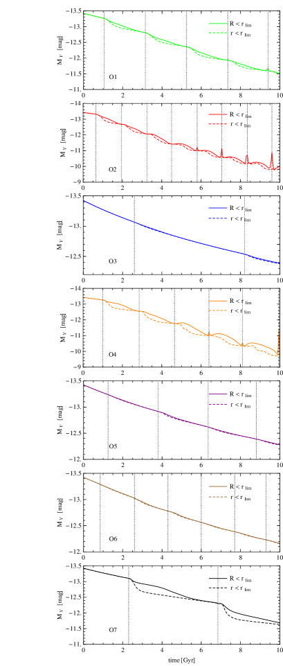
Figure 2.— The evolution of the total visual magnitude in time for simulations O1-O7. The dashed line shows measurements inside a sphere of radius $r_{\rm lim}$ centered on the dwarf where $r_{\rm lim}$ is the limiting radius containing all stars at the beginning of the simulation. The solid line shows measurements for an observer situated at the galactic center within the angular aperture corresponding to the projected radius $R=r_{\rm lim}$. Vertical dotted lines indicate pericenter passages.

3. Observing the dwarfs

3.1. The absolute magnitude

In order to estimate the observational parameters of the dwarfs we place an imaginary observer at the center of the Milky Way and introduce a spherical coordinate system centered on this point, with the radial coordinate along the line connecting the center of the Milky Way with the dwarf and the angles corresponding to celestial coordinates usually applied in astronomy. Since the dwarfs typically lose a substantial fraction of their stars the measurement of the total magnitude of the dwarf galaxy as a function of time is non-trivial as it is not a priori obvious which stars should be included as members of the dwarf at a given instant of the evolution. In real observations this measurement is done by integrating light up to a given radius or up to infinity if an analytical approximation of the light distribution is used. Here we adopt a simple approach of counting all stars included within some fixed limiting radius $r_{\rm lim}$. We adopt the value of this radius to be the distance from the center of the dwarf of the most distant star in the disk at the starting point of the evolution. The values of this radius are listed in the seventh column of Table LABEL:properties. This choice is physically well justified: all the stars that are beyond this radius at any later stage were ejected due to tidal forces.

Examples of the evolution of the total magnitude of the dwarf on orbits O1-O7 measured within radii $r<r_{\rm lim}$ from the center of the dwarf as a function of time are illustrated by dashed lines in Figure 2. The values were obtained by counting the stars within $r_{\rm lim}$, multiplying by the stellar mass and converting to the luminosity assuming a variable mass-to-light ratio for stars of $M/L_{V}=(1+0.15t)$M_⊙/L_⊙ in the visual band, where $t$ is the time from the start of the simulation, so that $M/L_{V}=1$M_⊙/L_⊙ at the start of the simulation (10 Gyr ago) and $M/L_{V}=2.5$M_⊙/L_⊙ at the end of the simulation (which we assume to correspond to the present time). This choice approximates well the evolution of the simple low-metallicity stellar population in the standard model described by Bruzual & Charlot (2003, their Figure 1). In this way we take into account the fading of the stellar population in time.

The evolution of the total magnitude determined in this way is very regular. Until the first pericenter passage in all cases the number of stars (and the stellar mass) remains constant and equal to the initial value (almost no stars are stripped beyond $r_{\rm lim}$) so the decreasing magnitudes are due entirely to the fading of the stellar population. In the runs on more eccentric orbits (O1, O2, O4 and O7) soon after each pericenter passage (marked by vertical dotted lines in Figure 2) the luminosity decreases due to the ejection of stars beyond $r_{\rm lim}$ by tidal forces, then declines more slowly again until the next pericenter. For the other runs this dependence on the orbital position would only be seen if we adopted a constant $M/L$ for the stars while in Figure 2 it is dominated by the fading of the stellar population. Note that the vertical scale is different in each panel of the Figure, e.g. many more stars are lost on the tightest orbit (O2) and the one with the smallest pericenter (O4) compared to the reference orbit O1 while very few are ejected on the most extended orbit O3.

An observer near the galactic center will obviously not be able to measure this intrinsic luminosity of the dwarfs but rather will count all the stars within the observation cone with the opening angle corresponding to $r_{\rm lim}$ at the distance of the dwarf. We assume that the distance of the dwarf is known perfectly (without any error) and the observer counts all stars within the projected radius $R<r_{\rm lim}$ corresponding to the angular distance from the center of the dwarf in the plane of the sky, which initially contained all the stars. The corresponding results for orbits O1-O7 are shown in Figure 2 as solid lines. For runs O3, O5 and O6, where the fading dominates, the result is almost identical, but for the other cases this measurement is biased with respect to the intrinsic one described above. Both measurements coincide at the pericenters of the orbits, but in other parts of the orbit (except for the initial part of the evolution) the estimated magnitudes are brighter for the realistic observations. This is due to the fact that near pericenters the tidal tails are oriented along the orbit, i.e. perpendicular to the line of sight of the observer, while near apocenters their orientation is more along the observer’s line of sight. This effect, described in more detail by Klimentowski et al. (2009b), is significantly stronger for orbits with higher eccentricity.

The second observational effect is the presence of the spikes, sudden increases of the measured magnitude at the later pericenter passages, well visible especially for O2 (second panel of Figure 2). These are the result of the particularly strong stellar mass loss for this tight orbit combined with a large opening angle of the observation cone at pericenters (the distance of the dwarf from the galactic center is then about 17 kpc while its assumed diameter is 12.5 kpc). At later times there is a lot of debris around the Milky Way stripped from the dwarf at earlier passages (see the orbit plotted with the red line in the upper panel of Figure 1) which are included in the observer’s field of view. Note that we include here all the debris stars without discriminating by distance (since distances are typically not known for individual stars) and most often the older debris lies quite far from the dwarf itself. These stars, if far enough, could in principle be excluded from the sample by careful analysis of the color-magnitude diagrams of the real dwarfs as they would cause a spread in luminosity. This effect would however have to be disentangled from the effects of star formation history (see e.g. the discussion for Leo I in Gallart et al. 1999, Sohn et al. 2007 and Mateo et al. 2008).

Given that galaxies on eccentric orbits spend a small fraction of the orbital time at pericenters and such small pericenter distances are probably not common among Milky Way satellites (e.g. Lux et al. 2010) this effect should be rare. It could in principle be observed e.g. for the Sagittarius dwarf if it had completed many pericentric passages around the Milky Way, which is unlikely (see Łokas et al. 2010b). In the following we will use the measured values at apocenters, where dwarfs are most likely to be seen, as most representative for the observed magnitudes. At these parts of the orbits the differences between the values measured by our observer ($R<r_{\rm lim}$) and the intrinsic ones ($r<r_{\rm lim}$) are never larger than 0.4 mag (for run O4) so the tidal tails do not seem to bias the measurements very strongly even for the most heavily stripped dwarfs.

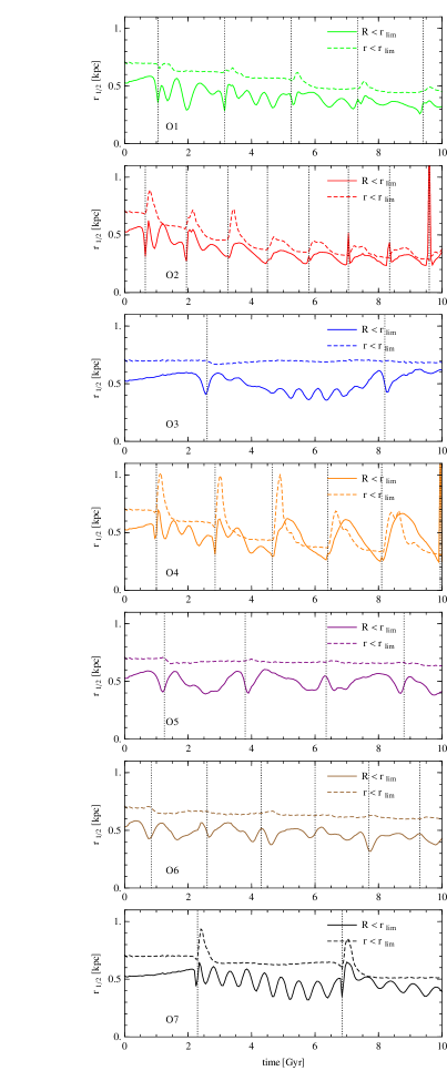
Figure 3.— The evolution of the half-light radius in time for simulations O1-O7. The dashed line shows measurements inside a sphere of radius $r_{\rm lim}$ centered on the dwarf where $r_{\rm lim}$ is the limiting radius containing all stars at the beginning of the simulation. The solid line shows measurements for an observer situated at the galactic center within the angular aperture corresponding to the projected radius $R=r_{\rm lim}$. Vertical dotted lines indicate pericenter passages.

3.2. The half-light radius

The next structural parameter of special interest is the half-light radius $r_{1/2}$. We first discuss the half-light radius measured in 3D, i.e. the radius containing half the total luminosity calculated from the number of stars contained within the 3D fixed radius $r<r_{\rm lim}$. Half-light radii determined in this way are plotted as dashed lines in Figure 3 for orbits O1-O7. The general trend, best seen for the tightest orbit O2, is that $r_{1/2}$ decreases with time on a large timescale, which reflects the decreasing size of the dwarf due to tidal stripping. Significant temporary increase of $r_{1/2}$ is however visible after each pericenter passage (indicated by vertical dotted lines in Figure 3), especially for runs O4, O7 and O2 with the smallest pericenters. This is due to the expansion of the dwarf’s stellar component in response to the tidal forces which are strongest at the pericenter.

A realistic measurement of $r_{1/2}$, by an observer located at the center of the Milky Way, would be done in 2D, on the surface of the sky and using the total luminosity determined within $R<r_{\rm lim}$. These measurements are shown in Figure 3 as solid lines. The half-light radii determined in this way are typically lower that their 3D counterparts which is due to the fact that the projected density profile of the stars is steeper, i.e. in the center of the dwarf all stars along the line of sight contribute and not only those that are close to the center in 3D. At later pericenters of simulation O2 the values of the projected $r_{1/2}$ show strong peaks. This is a direct consequence of the peaks in the measured total magnitudes due to large opening angles of the observation cone at these instances, as discussed above. Another feature of the evolution of the projected $r_{1/2}$ are wider bumps between pericenters, especially well visible in run O4 (but also present in O2), where the measured values of projected $r_{1/2}$ are about twice larger at apocenter than at pericenter. These are due to increased number of stars from the tidal tails that for this highly eccentric orbit are oriented along the observer’s line of sight for most of the time.

Another interesting observational effect that manifests itself in the measured values of the 2D half-light radii is their strong variability or even oscillation at the early stages of the evolution, especially visible after the first and second pericenter. As discussed in detail by K11, in most simulations studied here after the first pericenter the stellar disk transforms into a triaxial shape, usually a prolate spheroid or a bar which, as the evolution proceeds, becomes more spherical. The tumbling of the ellipsoid causes the observed variation of the measured $r_{1/2}$: when the observer’s line of sight is perpendicular to the major axis of the stellar component the dwarf appears more extended and the measured half-light radius is larger; when the major axis is aligned with the observer’s line of sight, the measured $r_{1/2}$ is smaller. This effect is strongest for simulation O7, but present even in the case of run O3 where a bar does not form and the stellar component is oblate, but still triaxial. Note that in the case of simulations O2 and O4, where the dwarf is particularly strongly stirred and its stellar component becomes almost spherical after the third pericenter, this variability of $r_{1/2}$ is no longer seen at these later stages and the variation of $r_{1/2}$ follows that of the total magnitude.

This interpretation of the measurements is confirmed by Figure 4 where we plot the angle between the major axis of the stellar component and the fixed $x$ axis of the simulation box which lies in the orbital plane of all simulations (at the initial configuration). The direction of the major axis was determined using all stars within a fixed radius of 0.6 kpc which corresponds to $(1-2)r_{1/2}$ in all cases. At all times we measured the angle between the $x$ axis and the dwarf’s major axis on the side of the dwarf which is closer to the $x$ axis so all angle values are between $0^{\circ}$ and $90^{\circ}$. The values of the angle were plotted starting from the first pericenter when the shape of the dwarf’s stellar component changes from the disk to the triaxial ellipsoid so that the major axis is well defined. For orbits O2 and O4 we do not show the measurements until the end because on these tight orbits the dwarf becomes almost spherical early on and the major axis is then no longer well defined again. The amplitude of the angle changes in some cases, which is due to the precession of the rotation axis. In addition, the rate at which the angle changes increases after the second pericenter for O1 which is due to speeding up of the figure rotation of the ellipsoid in this case, caused by the tidal force, as discussed by K11 (their section 5.2).

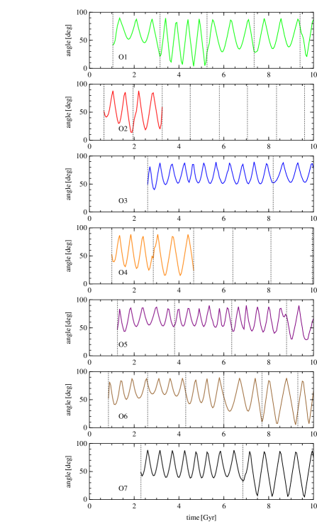
Figure 4.— The evolution of the angle between the major axis of the stellar component of the dwarf and the fixed $x$ axis of the simulation box in time for simulations O1-O7. Measurements are performed for stars within a fixed radius $r<0.6$ kpc. Vertical dotted lines indicate pericenter passages.

3.3. The central surface brightness

Another characteristic photometric property of dwarf galaxies is the central surface brightness $\mu_{V}$. This parameter does not have any 3D analog so we measure it directly in 2D by counting stars within $0.1r_{1/2}$ (where $r_{1/2}$ is the half-light radius determined in 2D) and dividing by the surface of the circle of this radius. This scale is about the closest to the center of the dwarf possible, i.e. the position of the innermost data point in measurements of surface brightness in real data. The results of this procedure are shown as solid lines in Figure 5 for runs O1-O7.

We notice a similar degree of variability in the measured surface brightness values as was observed for the 2D half-light radii. Since we measure the surface brightness within a fixed fraction of $r_{1/2}$ the two are obviously tightly related. Note that in the case of simulations O2 and O4 the strong variability at the early stages is replaced by an almost constant value between pericenters later on when the dwarf becomes spherical. The general trend is however to decrease the central surface brightness which means that the stars are stripped from all radii, not only from the outer parts i.e. the density profile of the stars is shifted down at all scales due to tidal stripping.

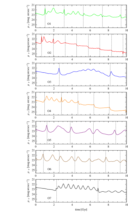
Figure 5.— The evolution of the central surface brightness in time for simulations O1-O7. Measurements are performed within $0.1r_{1/2}$ where $r_{1/2}$ is determined by an observer situated at the galactic center within the angular aperture corresponding to the projected radius $R=r_{\rm lim}$. Vertical dotted lines indicate pericenter passages.

3.4. Kinematics

One of the key parameters that distinguish dIrrs from dSphs is their $V/\sigma$ value, where $V$ is the rotation velocity and $\sigma$ is the (central) velocity dispersion of the stars. While dIrrs are believed to be rotationally supported, with $V/\sigma$ of the order of a few, dSphs usually exhibit much lower rotation levels with $V/\sigma$ below unity. However, contrary to common belief, dSphs are not in general completely devoid of rotation and it has been detected for many dSph galaxies, including Ursa Minor (Hargreaves et al. 1994; Armandroff et al. 1995), Carina (Muñoz et al. 2006), Sculptor (Battaglia et al. 2008), Leo I (Sohn et al. 2007; Mateo et al. 2008), Cetus (Lewis et al. 2007) and Tucana (Fraternali et al. 2009).

We measured $V$ and $\sigma$ using the following procedure, as close as possible to real observations. For each simulation output we selected stars, as seen by an observer at the galactic center, within projected radii $R<2r_{1/2}$ from the center of the dwarf, where $r_{1/2}$ are the 2D half-light radii determined above. This is approximately the region where kinematic measurements for dwarf galaxies are typically performed. We then determined the principal axes of the 2D distribution of the stars and rotated their positions in order to align the major axis of the dwarf image with the horizontal ($x$) axis. Figure 6 shows the distribution of (1 percent) of the stars within $R<2r_{1/2}$ obtained in this way for the configuration corresponding to the last apocenter for simulation O1.

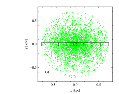
Figure 6.— The distribution of stars in simulation O1 within $2r_{1/2}$ as seen from the galactic center at the last apocenter of the orbit (green dots). The position of the stars were rotated so that the major axis of the galaxy image is along the $x$ axis. Only 1 percent of the stars is shown for clarity. The inner black circle of radius $0.1r_{1/2}$ encloses stars that are used in the determination of the central velocity dispersion. Black rectangles indicate eight bins along the major axis of the dwarf in which the rotation velocity and the velocity dispersion profiles are measured.

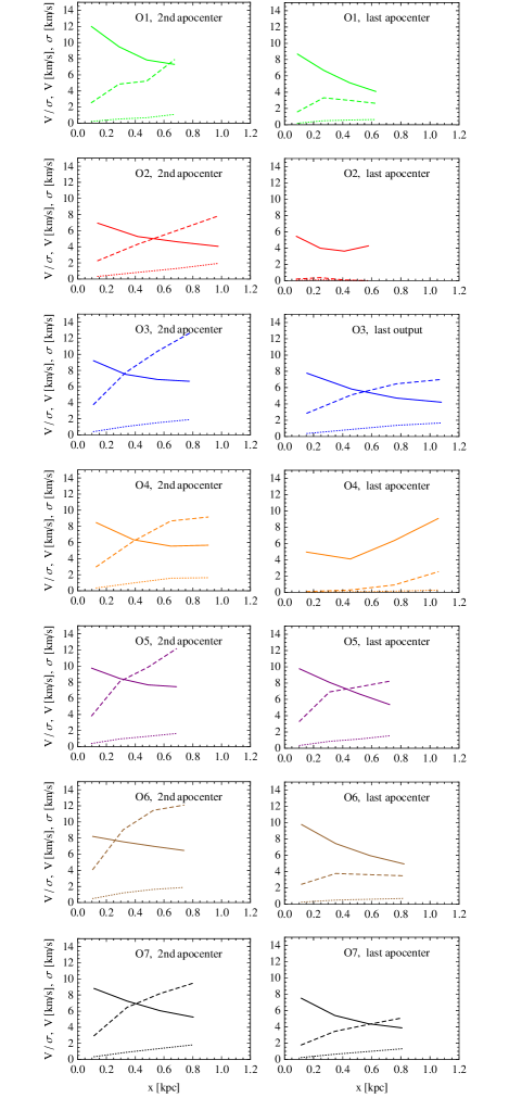
Figure 7.— The velocity dispersion profiles (solid lines), the rotation velocity profiles (dashed lines) and the ratios of the two (dotted lines) measured along the major axis of the observed dwarf for runs O1-O7 at their 2nd (left column) and last (right column) apocenters (except for the case O3 where the 2nd apocenter is the last so we plot the result for the final simulation output).

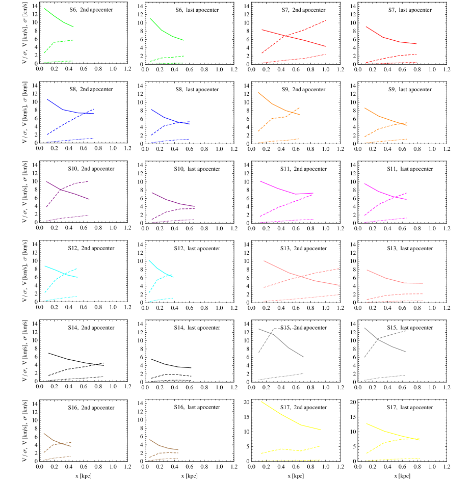
Figure 8.— The velocity dispersion profiles (solid lines), the rotation velocity profiles (dashed lines) and the ratios of the two (dotted lines) measured along the major axis of the observed dwarf for runs S6-S17 at their 2nd and last apocenters.

In order to estimate the central velocity dispersion of the dwarfs we selected for each output the stars within $R<0.1r_{1/2}$ (small black circle in Figure 6) and calculated the dispersion of radial velocity using standard estimators (see e.g. Łokas et al. 2005). By the choice of this innermost region we make sure that the sample is not contaminated by tidally stripped stars in the tails. Next, we select a narrow strip of stars along the major axis of the dwarf of size $0.1r_{1/2}\times 2r_{1/2}$ and sample the velocities of the stars in eight bins of size $0.1r_{1/2}\times 0.5r_{1/2}$ each. Since the outer bins are likely to be contaminated by tidally stripped stars we introduce a cut-off in velocities, i.e. we exclude the stars with velocities that differ from the dwarf’s systemic velocity by more than $3\sigma$ where $\sigma$ is the central velocity dispersion measured in the inner $R<0.1r_{1/2}$. Such a conservative cut-off is usually not sufficient for the reliable selection of stars for dynamical modelling (see Klimentowski et al. 2007, 2009b; Łokas et al. 2008; Łokas 2009) but seems stringent enough to measure basic kinematic properties of the dwarfs, as we aim to do here.

The results of these measurements for simulations O1-O7 and S6-S17 are shown in Figures 7 and 8 respectively for the outputs corresponding to the 2nd and the last apocenter (the left and right panel for each run). With dashed lines we plot the rotation velocity profiles and with solid lines the velocity dispersion profiles to illustrate their dependence on the distance from the center of the dwarf. Dotted lines give the ratio of the two values as a function of radius. All measurements were symmetrized, i.e. we show the average of two measurements on both sides of the dwarf. In most cases, the rotation profile decreases significantly between the 2nd and the last apocenter, while the dispersion remains roughly on the same level. This is due to the fact that tidal stirring causes the rotation to be replaced by random motions increasing the velocity dispersion, but at the same time dwarfs lose mass and the dispersion is decreased. The net outcome of these two effects is that the dispersion remains roughly constant in time.

All dispersion profiles look well-behaved, declining with radius, except for the case O4 (the right panel of the fourth row in Figure 7, orange line) where the dispersion profile shows a secondary increase at larger distances from the center. This is due to the contamination from the tidal tails that affects our measurements because the nominal half-light radius determined for this case is very large. As already discussed above, and seen in the fourth panel of Figure 3, in this case the $r_{1/2}$ values measured near apocenters at the later stages of evolution are about a factor of two larger than those at pericenters. Again, this is caused by the presence of tidal tails that for this very radial orbit ($r_{\rm apo}/r_{\rm peri}=10$, see Table LABEL:properties) for most of the time (except at the very pericenter) are oriented along the observer’s line of sight. The dwarf thus appears brighter and more extended (see also Figure 11 in Klimentowski et al. 2007). The contamination is also seen in the rotation curve (dashed orange line in the same panel of Figure 7) which shows tidally induced velocity gradient in the outer bins while no rotation is detected in the inner part for this very evolved dwarf.

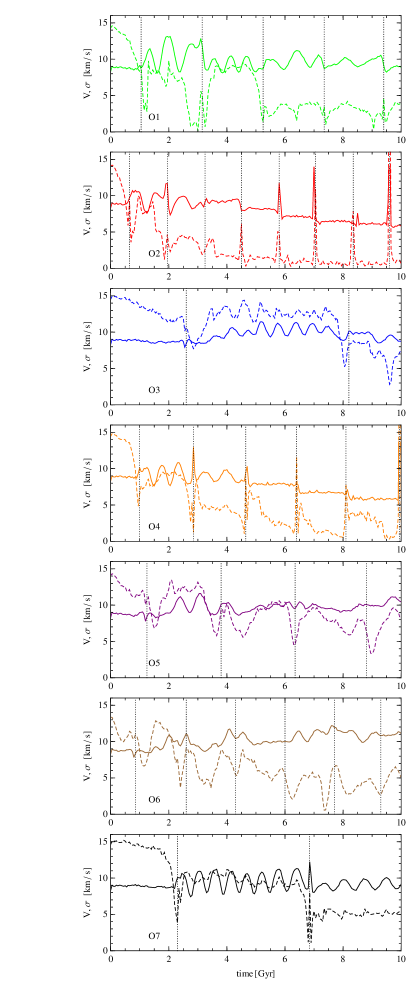
Figure 9.— The evolution of the central velocity dispersion (solid line) and the rotation velocity (dashed line) in time for simulations O1-O7. The central velocity dispersion was measured for stars with projected radii $R<0.1r_{1/2}$ and the rotation velocity was taken as a maximum value found along the major axis of the galaxy image within $2r_{1/2}$, as shown in the upper panel of Figure 6. Vertical dotted lines indicate pericenter passages.

Figure 9 shows the evolution of the kinematic properties in time for the seven simulations O1-O7 with different orbits. In each panel the measurements of the central velocity dispersion are plotted with solid lines while the values of the rotation velocity are shown with dashed lines. The values of rotation are taken as a maximum rotation velocity found along the rotation velocity profile (see Figures 7 and 8) measured along the major axis within $R<2r_{1/2}$. In simulations O2 and O4 where the dwarfs are most strongly affected by tidal forces, the contamination by tidal tails is well visible, although in a slightly different way in each run. For orbit O2 we see sharp increases of both velocity dispersion and rotation velocity at later pericenters caused by spikes in the measured values of $r_{1/2}$. In simulation O4, on the other hand, while the measured values of the central velocity dispersion remain unaffected (until the very last pericenter), the rotation velocity is overestimated when the dwarf is on its way from the pericenter to the apocenter. As discussed above, this is due to the overestimated value of $r_{1/2}$ which makes us probe the region well beyond the dwarf’s main stellar body.

Finally, it is worth noting that the tidal effects on the observables in runs O2 and O4, although in both cases due to tidally stripped stars, are of slightly different origin; while in O2 they are due to earlier wraps of tidally lost material (this run has more pericentric passages than any other orbit we considered), in O4 they are due to recently lost material residing in the tails oriented radially because of the high eccentricity of the orbit. In other runs the most characteristic feature of the kinematic measurements is the oscillation of the values (especially those of the central velocity dispersion) in simulations due, as discussed above, to the non-sphericity of the stellar distribution and the tumbling of its triaxial shape.

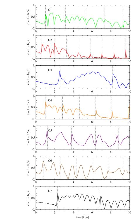
Figure 10.— The evolution of the ellipticity $e=1-b/a$ in time for simulations O1-O7. Measurements of the axis ratios $b/a$ are performed within $2r_{1/2}$ where $r_{1/2}$ is determined by an observer situated at the galactic center within the angular aperture corresponding to the projected radius $R=r_{\rm lim}$. Vertical dotted lines indicate pericenter passages.

3.5. Shapes

We conclude the measurements of the observational parameters of our simulated dwarfs by determining their shapes. For this purpose we select in each output the stars within projected radii $R<2r_{1/2}$ and rotate the 2D distribution to align the major axis of the galaxy image with $x$ and the minor axis with $y$, exactly as for the measurements of the kinematic properties. We then calculate the ellipticity parameter $e=1-b/a$ where $b/a$ is the axis ratio of the 2D distribution determined from the eigenvalues of the 2D inertia tensor.

The evolution of the ellipticity parameter $e$ in time is shown in Figure 10 for simulations O1-O7. Note that all runs start from the same value of $e=0.33$ which is due to the specific orientation of the dwarf galaxy disk at the beginning of the simulation. Namely, the disks are inclined by $45^{\circ}$ to the initial orbital plane and the initial velocity vector so the galaxy images appear elliptical to the observer at the center of the Milky Way. At later stages the ellipticity parameter displays strong variability due to the formation of the triaxial shape and tumbling of this shape, as well as the variability of the $2r_{1/2}$ scale inside which we measure the shape. A clear transition to sphericity is however seen for runs O2 and O4 where the ellipticity is very close to zero at the later stages of the evolution with momentary exceptions at pericenters where the scale $2r_{1/2}$ picks up some of the tidal tails oriented perpendicular to the line of sight at these instants.

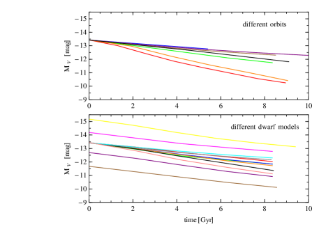
Figure 11.— The evolution of the total visual magnitude in time from the first to the last apocenter for different orbits (simulations O1-O7, upper panel) and different dwarf models (simulations S6-S17, lower panel).

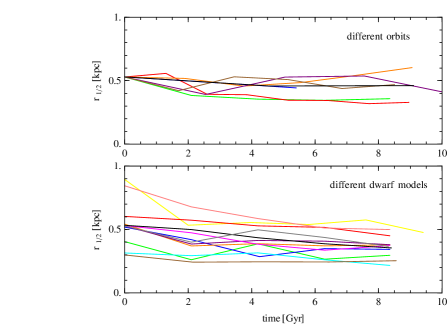
Figure 12.— The evolution of the half light radius in time from the first to the last apocenter for different orbits (simulations O1-O7, upper panel) and different dwarf models (simulations S6-S17, lower panel).

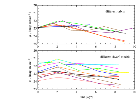
Figure 13.— The evolution of the central surface brightness in time from the first to the last apocenter for different orbits (simulations O1-O7, upper panel) and different dwarf models (simulations S6-S17, lower panel).

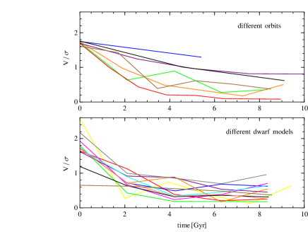
Figure 14.— The evolution of the ratio $V/\sigma$ in time from the first to the last apocenter for different orbits (simulations O1-O7, upper panel) and different dwarf models (simulations S6-S17, lower panel).

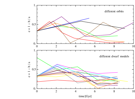
Figure 15.— The evolution of the ellipticity $e=1-b/a$ in time from the first to the last apocenter for different orbits (simulations O1-O7, upper panel) and different dwarf models (simulations S6-S17, lower panel).

4. Long-term evolution of the observed properties

In order to study the general trends in the evolution of the observational parameters in time in Figures 11-15 we plot the values measured previously only at subsequent apocenters, but for all simulations. In the upper panel of each figure we show with different colors the results for the simulations for different orbits and the same initial dwarf structure O1-O7, while in the lower panel we plot results for different initial structures of the dwarf and for the same default orbit S6-S17. A particular simulation can be identified by referring to the colors listed in the last column of Table LABEL:properties. The time of the last apocenter for each simulation can be found in the sixth column of the Table and the corresponding 2D values of the total magnitude $M_{V}$, half-light radius $r_{1/2}$, central surface brightness $\mu_{V}$, the ratio of the rotation velocity to the central velocity dispersion $V/\sigma$ and ellipticity $e=1-b/a$ measured at this last apocenter are listed in columns 8-12 of the Table.

The general trends in the evolution of the parameters are now clearly visible. As expected, the tidal stripping decreases the total magnitude of the dwarf and most so for the tightest orbit O2 and the one with the smallest pericenter and reasonably small orbital time O4. The trend of $r_{1/2}$ decreasing with time is less clear and more visible for dwarfs of different structure rather than on different orbits. Overall, the half-light radius remains remarkably constant over time, in contrast to the other characteristic scale-length of the dwarf, $r_{\rm max}$, where the maximum of the circular velocity occurs which was found by K11 to decrease very strongly during the evolution. This is not surprising, however, given that $r_{\rm max}$ is a characteristic scale-length of the total gravitational potential, which is dominated by dark matter, while $r_{1/2}$ characterizes the distribution of stars which are not so strongly affected by tidal forces.

The central surface brightness behaves differently from the other two properties discussed above. Typically, its value increases between the first and the second apocenter and then starts to decrease. This is due to the formation of the bar which in most cases occurs at the first pericenter and increases the density of the stars in the center of the dwarf. Later on, when the stellar distribution becomes more spherical and more stars are stripped, $\mu_{V}$ decreases as a function of time.

In Figure 14 we plot the ratio of the rotation velocity and the central velocity dispersion, $V/\sigma$, which measures the amount of ordered versus random motion of the stars. Both for different orbits and for different dwarf models the trend of $V/\sigma$ decreasing with time is clearly visible. This is one of the key signatures of tidal stirring and confirms that the process may indeed transform rotationally supported systems to those supported by random motions.

Finally, Figure 15 shows the trends in the evolution of the observed ellipticity. Here the trends are difficult to detect since a similar small ellipticity is measured for a disk close to face-on and a genuine almost spherical galaxy. In almost all our simulations the disk was initially inclined so that the measured ellipticity was $e=0.33$. The only exceptions are runs S6 where the disk is seen edge-on resulting in a large initial ellipticity $e=0.81$ (green line in the lower panel of Figure 15) and S7 where the disk is more face-on than the default orientation resulting in a small initial $e=0.18$ (red line in the lower panel of Figure 15). For different orbits the transition to the almost perfectly spherical shape is however reflected in very low $e$ values for runs O2 and O4, while for different dwarf models the ellipticity averaged over all runs is smaller than initially.

Table 2Properties of the dwarf galaxies of the Local Group.

Dwarf	Type	$M_{V}$	$r_{1/2}$	$\mu_{V}$	$V/\sigma$	$e=1-b/a$	References
galaxy		[mag]	[kpc]	[mag arcsec-2]
WLM	dIrr	$-14.5$	1.509	23.6	2.63	0.59	1,3
IC 10	dIrr	$-15.7$	0.775	22.1	3.75	0.3	1
NGC 147	dSph/dE	$-15.5$	0.753	21.6	1.0	0.46	1,2
NGC 185	dSph/dE	$-15.5$	0.521	20.1	0.63	0.26	1,2
LGS 3	dIrr/dSph	$-10.5$	0.312	25.6	0.22	0.26	1,3
IC 1613	dIrr	$-14.7$	1.870	23.5	2.47	0.24	1,3
Phoenix	dIrr/dSph	$-10.1$	–	–	0.22	0.3	1
UGCA 92	dIrr	$-12.6$	0.441	24.2	4.13	0.55	1,4
Leo A	dIrr	$-11.4$	0.341	–	0.32	0.40	1,19
Sextans B	dIrr	$-14.2$	0.417	22.9	1.22	0.23	1,3,4
NGC 3109	dIrr	$-15.7$	1.920	23.6	6.7	0.80	1
Antlia	dIrr/dSph	$-10.8$	0.672	24.3	–	0.35	1
Sextans A	dIrr	$-14.6$	1.068	23.7	2.38	0.21	1,3
GR 8	dIrr	$-11.6$	0.189	22.3	0.64	0.31	1
SagDIG	dIrr	$-12.3$	–	24.4	0.27	0.47	1
NGC 6822	dIrr	$-15.2$	0.582	21.4	5.88	0.47	1
Aquarius	dIrr/dSph	$-10.6$	0.342	23.6	0.76	0.40	1,18
IC 5152	dIrr	$-14.8$	–	–	3.88	0.18	1
UGCA 438	dIrr	$-12.0$	0.320	22.4	–	0.05	1,4
Pegasus	dIrr/dSph	$-12.9$	–	23.7	1.16	0.40	1,3
VV124	dIrr/dSph	$-12.4$	0.252	21.2	0.45	0.44	31
Carina	dSph	$-8.62$	0.241	25.5	0.43	0.33	1,5,6,7
Draco	dSph	$-8.74$	0.196	25.3	0.21	0.29	1,5,14,15
Fornax	dSph	$-13.03$	0.668	23.4	0.18	0.31	1,5,7
Leo I	dSph	$-11.49$	0.246	22.4	0.33	0.21	1,5,8
Leo II	dSph	$-9.60$	0.151	24.0	0.28	0.13	1,5,9
Sculptor	dSph	$-10.53$	0.260	23.7	0.30	0.32	1,5,7,10
Sextans	dSph	$-9.20$	0.682	26.2	0.48	0.35	1,5,7,11
Ursa Minor	dSph	$-8.42$	0.280	25.5	0.49	0.56	1,5,12,13
Sagittarius	dSph	$-13.3$	1.550	25.2	0.50	0.63	5,16,17
Andromeda I	dSph	$-11.8$	0.600	24.7	–	0.22	20
Andromeda II	dSph	$-12.6$	1.060	24.5	–	0.20	20
Andromeda III	dSph	$-10.2$	0.360	24.8	–	0.52	20
Andromeda V	dSph	$-9.6$	0.300	25.3	–	0.18	20
Andromeda VI	dSph	$-11.5$	0.420	24.1	–	0.41	20
Andromeda VII	dSph	$-13.3$	0.740	23.2	–	0.13	20
Cetus	dSph	$-11.3$	0.600	25.0	0.45	0.33	20,22
Tucana	dSph	$-9.5$	0.274	25.1	1.04	0.48	1,21,23
Andromeda IX	dSph	$-8.3$	0.530	26.8	–	0.25	21,25
Andromeda X	dSph	$-8.1$	0.339	26.7	–	0.44	21,25,26
Andromeda XIV	dSph	$-8.3$	0.413	–	–	0.31	21,27
Andromeda XV	dSph	$-9.4$	0.220	–	–	–	21
Andromeda XVI	dSph	$-9.2$	0.136	–	–	–	21
Andromeda XVII	dSph	$-8.5$	0.254	26.1	–	0.27	21,26,30
Andromeda XVIII	dSph	$-9.7$	0.363	25.6	–	–	29
Andromeda XIX	dSph	$-9.3$	2.065	29.3	–	0.17	29
Andromeda XXI	dSph	$-9.9$	0.875	27.0	–	0.20	28
Andromeda XXIII	dSph	$-10.2$	1.035	28.0	–	0.40	24
Andromeda XXV	dSph	$-9.7$	0.732	27.1	–	0.25	24
CVnI	dSph	$-8.6$	0.564	28.0	–	0.38	21,32
Leo T	dIrr/dSph	$-8.1$	0.115	26.9	–	0.1	21,33,34

5. Comparison with observations

The ultimate purpose of our study is to compare the measured observational parameters of the simulated dwarfs to real data. In Figures 16-19 we plot the central surface brightness $\mu_{V}$, the 2D half-light radius $r_{1/2}$, the kinematic parameter $V/\sigma$ and the ellipticity $e=1-b/a$ respectively as a function of the total magnitude of the simulated dwarfs at subsequent apocenters. The color coding of the simulations is the same as in previous Figures (see the last column of Table LABEL:properties) and again the upper panel is for dwarfs on different orbits while the lower one for dwarfs of different structure on the same default orbit. The direction of the lines from the left to the right, i.e. from the brighter to the fainter magnitudes, corresponds to the time flow because the total magnitude becomes fainter with time in all cases.

In Table  LABEL:realdwarfs we list the properties of dwarf galaxies of the Local Group with magnitudes in the range $-16<M_{V}<-8$ currently available in the literature. The columns give the galaxy name, the morphological type, the total visual magnitude, the half-light radius, the central surface brightness, the kinematic parameter $V/\sigma$ and the ellipticity parameter $e=1-b/a$. The references are provided in the last column of the Table. In cases where the exponential scale-lengths were only available, they were multiplied by a factor of 1.7 to approximate the half-light radius of the exponential profile. For the $V/\sigma$, the ‘raw’ values are used, i.e. those measured directly from the data, as we do for our simulated dwarfs, without correcting for inclination.

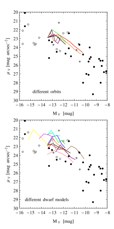
Figure 16.— The central surface brightness as a function of the total magnitude. Colored lines show the results for the simulated dwarfs at subsequent apocenters for different orbits (simulations O1-O7, upper panel) and different dwarf models (simulations S6-S17, lower panel). The evolution proceeds from the left to the right, from the brighter to the fainter magnitudes in all cases. In both panels the open circles show the data for dIrr galaxies, filled black circles the data for the dSph and dSph/dE galaxies and gray circles for transitory dIrr/dSph dwarfs. All data for the real dwarfs are listed in Table LABEL:realdwarfs.

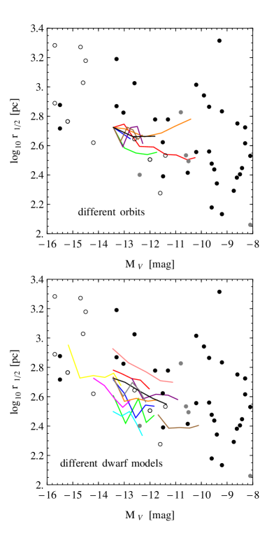
Figure 17.— Same as Figure 16 but for the half-light radius as a function of the total magnitude.

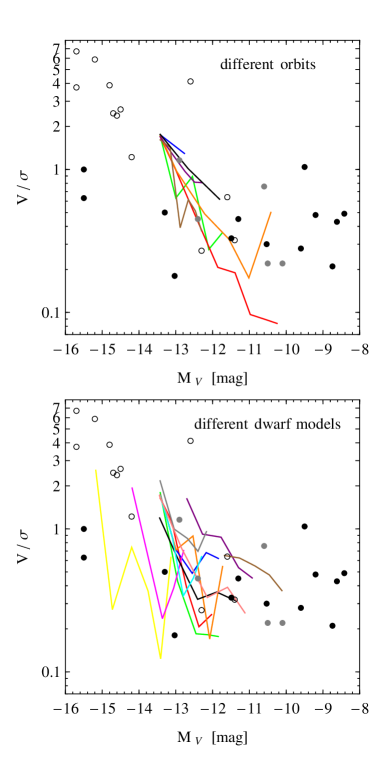
Figure 18.— Same as Figure 16 but for the kinematic parameter $V/\sigma$ as a function of the total magnitude.

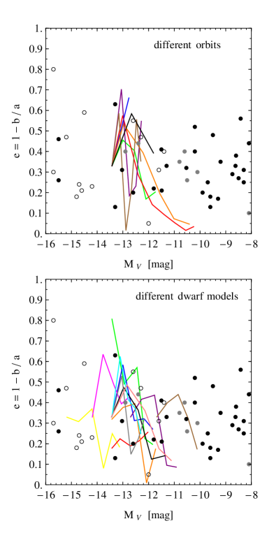
Figure 19.— Same as Figure 16 but for the ellipticity parameter $e=1-b/a$ as a function of the total magnitude.

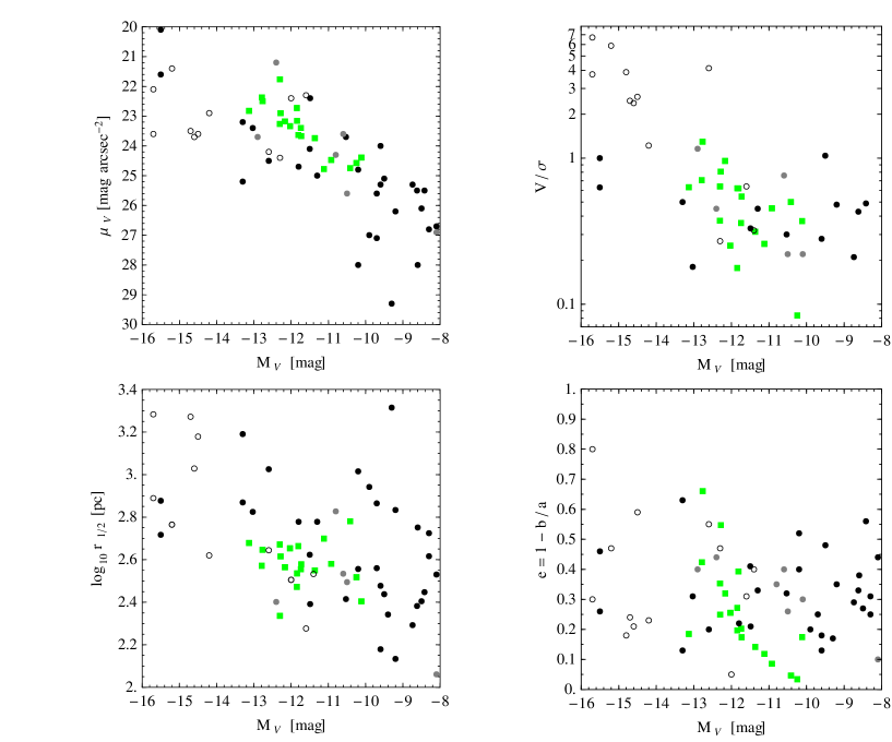
Figure 20.— The central surface brightness (upper left panel), the half-light radius (lower left panel), the $V/\sigma$ parameter (upper right panel) and the ellipticity (lower right panel) as a function of the total magnitude. Green squares show the measured parameters of the final products of tidal stirring in our simulations (at the last apocenter of their orbit). The open black circles show the data for dIrr galaxies, filled black circles the data for the dSph and dSph/dE galaxies and gray circles for transitory dIrr/dSph dwarfs from Table LABEL:realdwarfs.

The circles in Figures 16-19 show the real data for dwarf galaxies in the Local Group from Table LABEL:realdwarfs. The open circles mark the data for dIrr galaxies, filled black circles for the dSph and dSph/dE galaxies and gray circles for transitory dIrr/dSph dwarfs. The data in the $\mu_{V}$-$M_{V}$ and $r_{1/2}$-$M_{V}$ plots show strong correlation between the parameters (although in the latter case the scatter is much larger) demonstrating the trends of fainter galaxies to possess lower surface brightness and smaller size. There is also an obvious trend in $V/\sigma$-$M_{V}$: rotationally supported systems are typically brighter. The correlation is weakest in the $e$-$M_{V}$ plane due to the difficulty in relating the observed ellipticity to the real shape of a galaxy, as discussed above.

The evolutionary tracks of the simulated dwarfs in the $\mu_{V}$-$M_{V}$ plane (Figure 16) have a characteristic shape, similar for all simulations. While the magnitudes evolve towards the fainter end monotonically, the values of the surface brightness between the first and second apocenter increase and then mildly decrease at all subsequent apocenters. This later evolution traces very well the correlation between the observed values of the parameters for real Local Group dwarfs and is especially well visible in the case of runs O2 and O4 (the red and orange line in Figure 16) where the dwarfs are most affected by tides and therefore most evolved.

In the $r_{1/2}$-$M_{V}$ plane (Figure 17) the evolution of the simulated dwarfs shows more variety. Typically, the characteristic radii decrease strongly between the first and second pericenter, but in the later evolution they can also increase. Interestingly, because of the contamination by tidal tails, it can also happen for the most affected dwarfs, like the one of run O4 (the orange line in the upper panel of Figure 17), where $r_{1/2}$ increases during the later evolution, in contrast to the case of O2 (the red line). Overall, different orbits and different initial structures of the dwarf are able to reproduce the trends seen in the real data.

The direction of the evolution of the simulated dwarfs in the $r_{1/2}$-$M_{V}$ and especially in the $\mu_{V}$-$M_{V}$ plane strongly suggests that the observed correlations may be easily explained if dSph galaxies of the Local Group evolved from late-type dwarfs as predicted by the tidal stirring scenario. The trend of surface brightness decreasing with decreasing luminosity as observed in real dSph galaxies, in contrast to ellipticals, has been interpreted as pointing towards different formation scenarios of spheroidal and elliptical galaxies by Kormendy (1985) and Kormendy et al. (2009). They suggested that elliptical galaxies may form mostly via mergers while spheroidals are rather late-type systems that underwent transformation due to star-formation processes or environmental effects such as tidal stirring. This idea is supported by the analysis of the simulated Local Group by Klimentowski et al. (2010) who found that mergers of subhalos are rather rare in such systems and occur early on so they cannot significantly contribute to the formation of a large fraction of dSph galaxies. The tidal stirring scenario thus seems to be the most effective gravitational mechanism by which such objects could form.

6. Discussion

6.1. Observed versus intrinsic properties

Our results demonstrate the difficulty in determining the intrinsic properties of tidally stirred dwarf galaxies from the photometric and kinematic measurements alone. The interpretation of the observational biases in the photometric properties such as total magnitudes, half-light radii and central surface brightness is straightforward. All of them are affected by three issues: the presence of contamination by tidal tails, the non-sphericity of the stellar distribution and the ‘proximity effect’ that for strongly evolved dwarfs on orbits with small pericenters makes the observer seeing the dwarf at pericenter include more stars than are actually associated with the dwarf.

The measurements of kinematics and shapes are more complicated to interpret. Although in both these quantities the trend towards smaller $V/\sigma$ (signifying less rotation and more random motion in the stars) and towards more spherical shapes is clearly seen especially for more evolved dwarfs, these measurements depend critically on the initial orientation of the dwarf disks. This orientation was the same for all our simulations except S6 and S7 and may be considered ‘typical’ in the sense that our observer at the galactic center is able to detect both rotation and non-spherical shape of the stellar component at the initial state and later.

In particular, the cases O3, O5 and S15 classified as ‘non-dSph’ by K11 (see cases R3, R5 and R15 in their Table 2) based on their high intrinsic $V/\sigma>1$ (measured as the mean rotation around the shortest axis and the mean velocity dispersion for stars inside $r_{\rm max}$) also show high values of the order of unity in our measurements so they would be classified as transitory objects also by our observer. However, if the disk was seen exactly edge-on (as in run S6) the observer could identify it as rotating disk based on shape and rotation alone, while if it was face-on our observer would not be able to distinguish the disk from a spheroid supported by random motions. In real observations such cases can be morphologically classified by looking for additional signatures like the presence of gas or star formation regions.

Despite these difficulties, we emphasize that in this study we measured the properties of the simulated dwarfs in a realistic way so that they can be directly compared to real data. Figure 20 summarizes our results by showing as green squares the measured properties of the simulated dwarfs at the last apocenter in the $\mu_{V}$-$M_{V}$, $r_{1/2}$-$M_{V}$, $V/\sigma$-$M_{V}$ and $e$-$M_{V}$ planes. The circles display the data for dwarf galaxies of the Local Group from Table LABEL:realdwarfs as in Figures 16-19. The comparison proves that our dwarfs are indeed very similar to the real ones in those crucial parameters and thus shows that tidal stirring indeed can produce dSph galaxies from dIrr-like progenitors. Note that all our dwarfs (except two) initially had rather high masses of $10^{9}$ M_⊙ and therefore ended up on the more luminous side of the observed distribution. Starting from lower masses and luminosities we could easily reproduce also the less luminous dwarfs.

6.2. Comparison with earlier work

Observational parameters of the dSph galaxies produced by tidal stirring have already been discussed in the papers proposing the tidal stirring as a possible scenario for the formation of dSph galaxies by Mayer et al. (2001a,b). They have shown that the properties of the final products indeed follow the $\mu_{V}-M_{V}$ relation found for real dwarfs and that the $V/\sigma$ and ellipticity both decrease with time. Łokas et al. (2010a) measured the observational properties of dSph galaxies formed in three simulations discussed in Klimentowski et al. (2009a), similar to those studied here, and found them to depend strongly on the line of sight but still in the range characteristic of real dwarfs. In this work we improved on these earlier results by showing the actual evolutionary tracks of the dwarfs in different parameter planes and considering different observational biases caused by the observer’s position close to the galactic center.

Peñarrubia et al. (2008) studied the effect of tides on objects that were spherical from the start and constructed as stellar King profiles embedded in more extended dark halos. Understandably, their dwarfs do not undergo any morphological transformation and remain spherical and supported by random motions with no net rotation. Thus, they were unable to address such issues as the evolution of rotation or ellipticity. Their analysis was therefore restricted to such observational parameters as the total luminosity, the half-light radius, surface brightness and velocity dispersion. The evolutionary tracks of their spherical dwarfs in the $\mu_{V}$-$M_{V}$ and $r_{1/2}$-$M_{V}$ planes (their Figure 10) are similar as in our simulations (Figures 16-17), i.e. in both cases there is a clear trend of surface brightness and radii decreasing with decreasing luminosity of the dwarfs in time. Interestingly, the characteristic scales of the stellar distribution, quantified by the core radius of the King profile, were found there to evolve rather mildly and decrease only by about a factor of two, as in the case of our half-light radius.

Despite these similarities in the photometric properties, we find very different results concerning the evolution of the velocity dispersion and the mass-to-light ($M/L$) ratio. Since we were more interested in the evolution of the kinematic parameter $V/\sigma$ we do not show analogous plots for the dispersion alone, but the corresponding trends can be read from Figure 9 where both quantities, $V$ and $\sigma$, are plotted separately. Clearly, the central velocity dispersion decreases systematically only for the most strongly evolved dwarfs (O2 and O4), while it remains roughly constant for the other cases, in contrast to the findings of Peñarrubia et al. The evolution of the $M/L$ ratio as an intrinsic, rather than observational, parameter of our dwarfs was discussed already by K11: they found that tidal stripping typically decreases $M/L$ except for strongly evolved dwarfs where the dark halo has been truncated down to the stellar scales. Again, our results on this point are discrepant with those of Peñarrubia et al. who found $M/L$ increasing, making the dwarfs darker with time. The differences in the evolution are due to different initial conditions: in our case the stars are more tightly bound (especially after the formation of the bar) and are therefore more difficult to strip, keeping the velocity dispersion roughly constant and $M/L$ rather low. In the King models of Peñarrubia et al. the stars are weakly bound and easily stripped which decreases their dispersion and increases $M/L$. In summary, while the evolution of the photometric properties seems to be a general feature of tidal stripping, largely independent of the initial structure of the dwarfs, the kinematic and dynamical properties depend on the assumed dwarf model.

6.3. Conclusions

We have studied the observational parameters of simulated tidally stirred dwarf galaxies initially composed of disks embedded in extended dark matter halos. Our results build on and extend the previous study by K11, where intrinsic properties of the simulated dwarfs were discussed. Our main conclusions may be summarized as follows:

1. The photometric parameters, such as the absolute magnitude, the half-light radius and the central surface brightness as well as the kinematic properties can be reliably measured but are subject to a number of observational biases caused by the presence of tidally stripped stars and the non-sphericity of the stellar component.

2. The amount of bias in the measured quantities depends on the orbit and structural parameters of the dwarf but typically does not exceed 0.4 mag in total visual magnitude and a factor of two in half-light radius. Rotation can be overestimated for strongly stripped dwarfs on eccentric orbits even if a $3\sigma$ cut-off is applied to radial velocities.

3. The effects of tidal stirring manifest themselves by decreasing the observed total magnitude, the half-light radius, the central surface brightness, rotation and ellipticity in time, while the central velocity dispersion remains roughly constant except for the most heavily stripped dwarfs where it also decreases due to strong mass loss.

4. The correlations between the observational parameters of the simulated dwarfs reveal strong similarity to those in the real data. The evolutionary tracks of the tidally stirred dwarfs move them from regions characteristic for dIrr galaxies to those typical for dSph galaxies of the Local Group. This behavior corroborates the existence of a connection between these two types of objects and therefore strongly supports the tidal stirring model as a possible scenario of their evolution.

References

- Armandroff et al. (1995) Armandroff, T. E., Olszewski, E. W., & Pryor, C. 1995, AJ, 110, 2131
- Battaglia et al. (2008) Battaglia, G., Helmi, A., Tolstoy, E., Irwin, M., Hill, V., & Jablonka, P. 2008, ApJ, 681, L13
- Battaglia et al. (2011) Battaglia, G., Tolstoy, E., Helmi, A., Irwin, M., Parisi, P., Hill, V., & Jablonka, P. 2011, MNRAS, 411, 1013
- Bellazzini et al. (2011) Bellazzini, M., et al. 2011, A&A, 527, A58
- Brasseur et al. (2011) Brasseur, C. M., Martin, N. F., Rix, H. W., Irwin, M., Ferguson, A. M. N., McConnachie, A. W., & de Jong, J. 2011, ApJ, 729,23
- Bruzual & Charlot (2003) Bruzual, G., & Charlot, S. 2003, MNRAS, 344, 1000
- Bullock et al. (2000) Bullock, J. S., Kravtsov, A. V., & Weinberg, D. H. 2000, ApJ, 539, 517
- de Jong et al. (2008) de Jong, J. T. A., et al. 2008, ApJ, 680, 1112
- D’Onghia et al. (2009) D’Onghia, E., Besla, G., Cox, T. J., & Hernquist, L. 2009, Nature, 460, 605
- Fraternali et al. (2009) Fraternali, F., Tolstoy, E., Irwin, M. J., & Cole, A. A. 2009, A&A, 499, 121
- Gallart et al. (1999) Gallart, C., et al. 1999, ApJ, 514, 665
- Geha et al. (2010) Geha, M., van der Marel, R. P., Guhathakurta, P., Gilbert, K. M., Kalirai, J., & Kirby, E. N. 2010, ApJ, 711, 361
- Hargreaves et al. (1994) Hargreaves, J. C., Gilmore, G., Irwin, M. J., & Carter, D. 1994, MNRAS, 271, 693
- Hernquist (1990) Hernquist, L. 1990, ApJ, 356, 359
- Hunter et al. (2010) Hunter, D. A., Elmegreen, B. G., & Ludka, B. C. 2010, AJ, 139, 447
- Irwin et al. (2007) Irwin, M. J., et al. 2007, ApJ, 656, L13
- Irwin et al. (2008) Irwin, M. J., Ferguson, A. M. N., Huxor, A. P., Tanvir, N. R., Ibata, R. A., & Lewis, G. F. 2008, ApJ, 676, L17
- Kalirai et al. (2010) Kalirai, J. S., et al. 2010, ApJ, 711, 671
- Kazantzidis et al. (2004) Kazantzidis, S., Mayer, L., Mastropietro, C., Diemand, J., Stadel, J. & Moore, B. 2004, ApJ, 608, 663
- Kazantzidis et al. (2011) Kazantzidis, S., Łokas, E. L., Callegari, S., Mayer, L., & Moustakas, L. A. 2011, ApJ, 726, 98 (K11)
- Kleyna et al. (2002) Kleyna, J., Wilkinson, M. I., Evans, N. W., Gilmore, G., & Frayn, C. 2002, MNRAS, 330, 792
- Klimentowski et al. (2007) Klimentowski, J., Łokas, E. L., Kazantzidis, S., Prada, F., Mayer, L., & Mamon, G. A. 2007, MNRAS, 378, 353
- Klimentowski et al. (2009a) Klimentowski, J., Łokas, E. L., Kazantzidis, S., Mayer, L., & Mamon, G. A. 2009a, MNRAS, 397, 2015
- Klimentowski et al. (2009b) Klimentowski, J., Łokas, E. L., Kazantzidis, S., Mayer, L., Mamon, G. A., & Prada, F. 2009b, MNRAS, 400, 2162
- Klimentowski et al. (2010) Klimentowski, J., Łokas, E. L., Knebe, A., Gottlöber, S., Martinez-Vaquero, L. A., Yepes, G., & Hoffman, Y. 2010, MNRAS, 402, 1899
- Koch et al. (2007) Koch, A., Kleyna, J. T., Wilkinson, M. I., Grebel, E. K., Gilmore, G. F., Evans, N. W., Wyse, R. F. G., & Harbeck, D. R. 2007, AJ, 134, 566
- Kormendy (1985) Kormendy, J. 1985, ApJ, 295, 73
- Kormendy et al. (2009) Kormendy, J., Fisher, D. B., Cornell, M. E., & Bender, R. 2009, 182, 216
- Lewis et al. (2007) Lewis, G. F., Ibata, R. A., Chapman, S. C., McConnachie, A., Irwin, M. J., Tolstoy, E., & Tanvir, N. R. 2007, MNRAS, 375, 1364
- Lokas (2009) Łokas, E. L. 2009, MNRAS, 394, L102
- Lokas et al. (2005) Łokas, E. L., Mamon, G. A., & Prada, F. 2005, MNRAS, 363, 918
- Lokas et al. (2008) Łokas, E. L., Klimentowski, J., Kazantzidis, S., & Mayer, L. 2008, MNRAS, 390, 625
- Łokas et al. (2010a) Łokas, E. L., Kazantzidis, S., Klimentowski, J., Mayer, L., & Callegari, S. 2010a, ApJ, 708, 1032
- Łokas et al. (2010b) Łokas, E. L., Kazantzidis, S., Majewski, S. R., Law, D. R., Mayer, L., & Frinchaboy, P. M. 2010b, ApJ, 725, 1516
- Łokas et al. (2010c) Łokas, E. L., Kazantzidis, S., Mayer, L., & Callegari, S. 2010c, in Proc. JENAM 2010 Symposium 2, Environment and the formation of galaxies: 30 years later, ed. I. Ferreras, & A. Pasquali, in press, arXiv:1011.3357
- Lux et al. (2010) Lux, H., Read, J. I., & Lake, G. 2010, MNRAS, 406, 2312
- Majewski et al. (2003) Majewski, S. R., Skrutskie, M. F., Weinberg, M. D., & Ostheimer, J. C. 2003, ApJ, 599, 1082
- Majewski et al. (2007) Majewski, S. R., et al. 2007, ApJ, 670, L9
- Martin et al. (2009) Martin, N. F., et al. 2009, ApJ, 705, 758
- Mateo (1998) Mateo, M. L. 1998, ARA&A, 36, 435
- Mateo et al. (2008) Mateo, M., Olszewski, E. W., & Walker, M. G. 2008, ApJ, 675, 201
- Mayer et al. (2001a) Mayer, L., Governato, F., Colpi, M., Moore, B., Quinn, T., Wadsley, J., Stadel, J., & Lake, G. 2001a, ApJ, 547, L123
- Mayer et al. (2001b) Mayer, L., Governato, F., Colpi, M., Moore, B., Quinn, T., Wadsley, J., Stadel, J., & Lake, G. 2001b, ApJ, 559, 754
- Mayer et al. (2006) Mayer, L., Mastropietro, C., Wadsley, J., Stadel, J. & Moore, B. 2006, MNRAS, 369, 1021
- Mayer et al. (2007) Mayer, L., Kazantzidis, S., Mastropietro, C., & Wadsley, J. 2007, Nature, 445, 738
- Mayer (2010) Mayer, L. 2010, Advances in Astronomy, Vol. 2010, 278434
- McConnachie & Irwin (2006) McConnachie, A. W., & Irwin, M. J. 2006, MNRAS, 365, 1263
- McConnachie et al. (2006) McConnachie, A. W., Arimoto, N., Irwin, M., & Tolstoy, E. 2006, MNRAS, 373, 715
- McConnachie et al. (2008) McConnachie, A. W., et al. 2008, ApJ, 688, 1009
- Mo et al. (1998) Mo, H. J., Mao, S., & White, S. D. M. 1998, MNRAS, 295, 319
- Moore et al. (1996) Moore, B., Katz, N., Lake, G., Dressler, A., & Oemler, A. 1996, Nature, 379, 613
- Muñoz et al. (2005) Muñoz, R. R., et al. 2005, ApJ, 631, L137
- Muñoz et al. (2006) Muñoz, R. R., et al. 2006, ApJ, 649, 201
- Navarro et al. (1996) Navarro, J. F., Frenk, C. S., & White, S. D. M. 1996, ApJ, 462, 563 (NFW)
- Peñarrubia et al. (2008) Peñarrubia, J., Navarro, J. F., & McConnachie, A. W. 2008, ApJ, 673, 226
- Richardson et al. (2011) Richardson, J. C., et al. 2011, ApJ, 732, 76
- Ricotti & Gnedin (2005) Ricotti, M., & Gnedin, N. Y. 2005, ApJ, 629, 259
- Sawala et al. (2010) Sawala, T., Scannapieco, C., Maio, U., & White, S. D. M. 2010, MNRAS, 402, 1599
- Sharina et al. (2008) Sharina, M. E., et al. 2008, MNRAS, 384, 1544
- Sohn et al. (2007) Sohn, S. T., et al. 2007, ApJ, 663, 960
- Stadel (2001) Stadel, J. G. 2001, PhD thesis, Univ. of Washington
- Susa & Umemura (2004) Susa, H., & Umemura, M. 2004, ApJ, 610, L5
- Tassis et al. (2000) Tassis, K., Kravtsov, A. V., & Gnedin, N. Y., 2008, ApJ, 672, 888
- Tolstoy et al. (2009) Tolstoy, E., Hill, V., & Tosi, M. 2009, ARA&A, 47, 371
- Vansevičius et al. (2004) Vansevičius, V., et al. 2004, ApJ, 611, L93
- Walker et al. (2010) Walker, M. G., Mateo, M., Olszewski, E. W., Peñarrubia, J., Evans, W. N., & Gilmore, G. 2010, ApJ, 710, 886
- Widrow & Dubinski (2005) Widrow, L. M., & Dubinski, J. 2005, ApJ, 631, 838
- Wilkinson et al. (2004) Wilkinson, M. I., Kleyna, J. T., Evans, N. W., Gilmore, G. F., Irwin, M. J., & Grebel, E. K. 2004, ApJ, 611, L21
- Zucker et al. (2006) Zucker, D. B., et al. 2006, ApJ, 643, L103
- Zucker et al. (2007) Zucker, D. B., et al. 2007, ApJ, 659, L21