Elliptic flow of the dilute Fermi gas: From kinetics to hydrodynamics

Abstract

We use the Boltzmann equation in the relaxation time approximation to study the expansion of a dilute Fermi gas at unitarity. We focus, in particular, on the approach to the hydrodynamic limit. Our main finding are: i) In the regime that has been studied experimentally hydrodynamic effects beyond the Navier-Stokes approximation are small, ii) mean field corrections to the Boltzmann equation are not important, iii) experimental data imply that freezeout occurs very late, that means that the relaxation time remains smaller than the expansion time during the entire evolution of the system, iv) the experimental results also imply that the bulk viscosity is significantly smaller than the shear viscosity of the system.

I Introduction

The dilute Fermi gas at unitarity is a strongly correlated quantum fluid that serves as a new paradigm for strong correlations in many other systems, like dilute neutron matter, the quark-gluon plasma, and high $T_{c}$ superconductors Bloch:2007 ; Giorgini:2008 ; Chin:2009 ; Schafer:2009dj . The interest in the unitary Fermi gas derives in large part from the fact that the system provides a particularly simple realization of strong correlations. At unitarity the $s$-wave scattering length is infinite, and the effective range and all other scattering parameters are zero. This implies that even though the system is very strongly correlated, details of the interaction are not important and the fluid is scale invariant.

An important manifestation of strong correlations is the observation of nearly ideal hydrodynamic flow OHara:2002 . Recently, a significant amount of effort has been devoted to quantifying this observation by determining the shear viscosity $\eta$ or the dimensionless ratio of shear viscosity to entropy density $\eta/s$ Schafer:2007pr ; Turlapov:2007 ; Schaefer:2009px ; Thomas:2009zz ; Cao:2010 . This effort is inspired, in part, by the conjecture that there is a universal lower bound on the shear viscosity to entropy density of strongly coupled fluids Kovtun:2004de , and by similar measurements of $\eta/s$ for the quark gluon plasma created in heavy ion collisions at RHIC and the LHC rhic:2005 ; Romatschke:2007mq ; Dusling:2007gi ; Song:2008hj .

Measurements of the shear viscosity of the unitary Fermi gas are based on using viscous hydrodynamics to analyze the expansion of a gas cloud after the confining potential is removed. Alternatively, one can study collective oscillations of the cloud. The main difficulty with these analyses is that hydrodynamics breaks down in the dilute corona of the trapped gas, and that dissipative corrections from this regime can potentially be large. It is therefore important to study the crossover from weakly collisional kinetic dynamics to almost ideal hydrodynamics.

In this paper we use the Boltzmann (and Boltzmann-Vlasov) equation in the relaxation time approximation to study a number of issues related to the crossover from kinetics to hydrodynamics. In Sect. II we discuss the matching between the Boltzmann equation and the Navier-Stokes equation for a simple functional form of the relaxation time. We also study, for the system parameters realized in the recent experiments of Cao et al. Cao:2010 , the magnitude of hydrodynamic effects beyond the Navier-Stokes approximation. In Sect. III we investigate the role of mean field effects in the Boltzmann-Vlasov equation. In Sect. IV we study the question whether there is any experimental evidence for freezeout, that is a transition between hydrodynamic and ballistic expansion during the evolution of the system. In Sect. V we study a more realistic model of the relaxation time, and in Sect. VI we study the possible role of bulk viscosity. We should note that there is an extensive literature on using the Boltzmann equation to describe the dynamics of trapped Bose and Fermi gases, see for example Guery:1999 ; Pedri:2002 ; Guery:2002 ; Menotti:2002 ; Jackson:2004 ; Nikuni:2004 ; Bruun:2005 ; Bruun:2006 ; Bruun:2007 . In this paper we focus, in particular, on the questions how close recent experiments are to the hydrodynamic limit, and how large the associated uncertainties in the shear viscosity are.

II Boltzmann equation in relaxation time approximation

We consider the limit in which the unitary Fermi gas can be described in terms of a quasi-particle distribution function $f(x,v,t)$. The equation of motion for the distribution function is the Boltzmann-Vlasov equation

$$\frac{\partial f}{\partial t}+v_{i}\frac{\partial f}{\partial x_{i}}-\frac{1}{m}\frac{\partial(U_{\it mf}+U_{\it ext})}{\partial x_{i}}\frac{\partial f}{\partial v_{i}}=C[f]\,,$$ (1)

where $U_{\it ext}=(m/2)\omega_{i}^{2}x_{i}^{2}$ is the external confinement potential, $U_{\it mf}$ is a mean field potential, and $C[f]$ is the collision term. We will study the effect of the mean field potential in Sect. III. For now we will set $U_{\it mf}=0$. Throughout this paper we will approximate the collision term using the relaxation time approximation

$$C[f]\simeq-\frac{f-f_{\it le}}{\tau}\,,$$ (2)

where $\tau$ is the relaxation time and $f_{\it le}$ is the local equilibrium distribution. The relaxation time does not have to be a constant, and we will study different scaling laws for $\tau$ below.

We are interested in the time evolution of a harmonically trapped cloud after the trapping potential is removed. We will follow Pedri:2002 ; Guery:2002 and use a scaling ansatz for the distribution function

$$f(x,v,t)=\Gamma(t)f_{0}(R(t),U(t))$$ (3)

with

$$R_{i}=\frac{x_{i}}{b_{i}}\,,\hskip 14.22636ptU_{i}=\frac{v_{i}-\frac{\dot{b}_{i}}{b_{i}}x_{i}}{\theta_{i}^{1/2}}\,,\hskip 14.22636pt\Gamma=\prod_{j}\frac{1}{b_{j}\theta_{j}^{1/2}}\,,$$ (4)

where $b_{i},\theta_{i}$ are functions of $t$ and $f_{0}(r,v)$ is a solution of the Boltzmann-Vlasov equation in equilibrium

$$v_{i}\frac{\partial f_{0}}{\partial x_{i}}=\frac{1}{m}\frac{\partial(U_{\it mf}+U_{\it ext})}{\partial x_{i}}\frac{\partial f_{0}}{\partial v_{i}}\,.$$ (5)

In the absence of a mean field potential this equation is solved by a Maxwell distribution. The scaling ansatz (3) breaks local thermal equilibrium only through the anisotropy of the temperature parameters $\theta_{i}$. The corresponding local equilibrium distribution $f_{\it le}$ can be found by replacing $\theta_{i}\to\bar{\theta}=(\sum_{i}\theta_{i})/3$. This distribution function is characterized by having the same mean kinetic energy as the non-equilibrium distribution $f$. In the free streaming limit $\tau\to\infty$ equ. (3) solves the Boltzmann equation exactly. In the presence of collisions we can obtain a differential equation for the parameters $b_{i}(t)$ and $\theta_{i}(t)$ by computing moments of the Boltzmann equation. Integrating the Boltzmann equation over $\int d^{3}U\,d^{3}R\,U_{j}R_{j}$ (no sum over $j$) gives Pedri:2002

$$\ddot{b}_{j}+\omega_{j}^{2}b_{j}-\omega_{j}^{2}\frac{\theta_{j}}{b_{j}}=0\,.$$ (6)

The second term is due to the external potential and is not present if one considers an expanding cloud. Taking moments of the form $\int d^{3}U\,d^{3}R\,U_{j}U_{j}$ gives

$$\dot{\theta}_{j}+2\frac{\dot{b}_{j}}{b_{j}}\theta_{j}=-\frac{1}{\tau}\left(\theta_{j}-\bar{\theta}\right)\,.$$ (7)

Taking moments weighted with $R_{j}R_{j}$ does not provide additional constraints. Together with the initial conditions $b_{j}(0)=\theta_{j}(0)=1$ and $\dot{b}_{j}(0)=0$ equations (6,7) describe the evolution of an expanding cloud.

We expect the Boltzmann equation to reduce to hydrodynamics in the limit that the relaxation time is shorter than the expansion time, $\tau\ll\tau_{\it exp}=(\sum_{i}\dot{b}_{i}/b_{i})^{-1}$. In the limit $\tau\to 0$ equ. (7) implies that $\theta_{i}=\bar{\theta}$ and $\bar{\theta}=(\prod_{i}b_{i})^{-2/3}$. The equation of motion for the scale parameter of an expanding cloud reduces to

$$\ddot{b}_{i}-\frac{\omega_{i}^{2}}{b_{i}\prod_{j}b_{j}^{2/3}}=0\,.$$ (8)

This equation is identical to the equation of motion that follows from the Euler equation in ideal hydrodynamics Menotti:2002 ; Schaefer:2009px . If we keep terms of order $\tau$ we recover dissipative terms in hydrodynamics. For this purpose we compute the conserved charges (mass, momentum, and energy) and the associated currents. The mass density is given by $\rho=mn=m\int d^{3}vf(x,v,t)$. The momentum density is

$$g_{i}=m\int d^{3}v\,v_{i}f(x,v,t)=\rho V_{i}\,$$ (9)

where $V_{i}=(\dot{b}_{i}/b_{i})x_{i}$ is the local fluid velocity. The energy density is

$${\cal E}=\frac{1}{2}\int d^{3}v\,mv^{2}f(x,v,t)=\frac{1}{2}\rho V^{2}+n\epsilon_{0}\,,$$ (10)

with $\epsilon_{0}=\frac{3}{2}T_{\it le}$. The stress tensor is given by

$$\Pi_{ij}=\int d^{3}v\,mv_{i}v_{j}f(x,v,t)=\rho V_{i}V_{j}+\delta_{ij}\rho\theta_{i}\langle v_{i}^{2}\rangle\,,$$ (11)

where $\langle v_{i}^{2}\rangle={\cal V}^{-1}\int d^{3}v\,f_{0}(R,v)$ with ${\cal V}=\prod_{i}b_{j}$ is an average with respect to the equilibrium distribution in the local rest frame. We can write $f=f_{\it le}+\delta f$ and split equ. (11) into a local equilibrium and dissipative part. The dissipative part is

$$\delta\Pi_{ij}=-\delta_{ij}nT_{\it le}\left(1-\frac{\theta_{i}}{\bar{\theta}}\right)\,.$$ (12)

We can use equ. (7) to express $\theta_{i}/\bar{\theta}$ in terms of $\theta_{i}$ and $b_{i}$. The result is explicitly proportional to $\tau$, so that at leading order we can use the relation between $\theta_{i}$ and $b_{i}$ in ideal hydrodynamics. We find

$$\delta\Pi_{ij}=-\delta_{ij}nT_{\it le}\tau\left(2\frac{\dot{b_{i}}}{b_{i}}-\frac{2}{3}\sum_{k}\frac{\dot{b_{k}}}{b_{k}}\right)\,.$$ (13)

Using $V_{i}=x_{i}(\dot{b}_{i}/b_{i})$ we see that equ. (13) matches the viscous stress tensor in hydrodynamics, $\delta\Pi_{ij}=-\eta(\partial_{i}V_{j}+\partial_{j}V_{i}-\frac{2}{3}\delta_{ij}(\partial\cdot V))-\zeta\delta_{ij}(\partial\cdot V)$, if we set

$$\eta=n\tau T_{\it le}\,,$$ (14)

and $\zeta=0$. Equ. (14) is a standard result in kinetic theory Bruun:2005 . The bulk viscosity is expected to vanish in the dilute Fermi gas at unitarity Son:2005tj ; Enss:2010qh , but we will see that the relaxation time approximation leads to a vanishing bulk viscosity even in cases where we expect the physical result to be non-zero. Scale invariance also implies that $\eta=n\alpha_{n}(y)$, where $\alpha_{n}$ is a function of $y=mT/n^{2/3}$, and $\tau=\tau_{n}(y)/T$. The matching condition (14) then implies that $\tau_{n}(y)=\alpha_{n}(y)$. The simplest case is that $\alpha_{n}$ is a constant. In this case the relaxation time is only a function of temperature $\tau=\alpha_{n}/T_{\it le}=\alpha_{n}/(T_{0}\bar{\theta})$, where $T_{0}$ is the initial temperature.

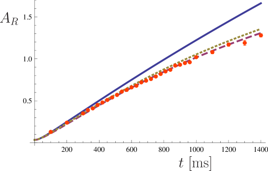
Figure 1: This figure shows the matching between kinetic theory and Navier-Stokes hydrodynamics. We show the evolution of the aspect ratio $A_{R}$ as a function of time. The solid points are data taken at an initial energy $E/E_{F}=3.61$ Cao:2010 . The solid line shows a solution of the Euler equation, the long dashed line is a solution of the Navier-Stokes equation where the viscosity coefficient $\alpha_{n}=22.1$ ($\eta=\alpha_{n}n$) was adjusted to reproduce the data, and the short-dashed line is a solution to the Boltzmann equation in the relaxation time approximation with $\tau=\alpha_{n}/T$.

In Fig. 1 we compare the solution of the Boltzmann equation to a solution of the Navier-Stokes equation. The Navier-Stokes solution is described in Schafer:2010dv , and the parameter $\alpha_{n}$ was fitted to data taken by Cao et al. Cao:2010 at an initial energy $E/E_{F}=3.61$, where $E_{F}=(3N)^{1/3}\bar{\omega}$. The experiment involves an axially symmetric trap with $\omega_{\perp}\equiv\omega_{x}=\omega_{y}$. The trap frequencies are $\omega_{\perp}/(2\pi)=5078.7$ Hz and $\omega_{z}/(2\pi)=175.7$ Hz, the number of particles is $N=2.61\cdot 10^{5}$ and we have defined $\bar{\omega}=\lambda^{1/3}\omega_{\perp}$ with $\lambda=\omega_{z}/\omega_{\perp}$. The relaxation time was fixed according to the relation $\tau_{n}=\alpha_{n}$. Fig. 1 shows the time evolution of the aspect ratio $A_{R}(t)=b_{\perp}(t)/b_{z}(t)$. We observe that the difference between the kinetic theory calculation and Navier-Stokes hydrodynamics is indeed small, indicating that in the regime that has been studied experimentally higher order hydrodynamic effects are small.

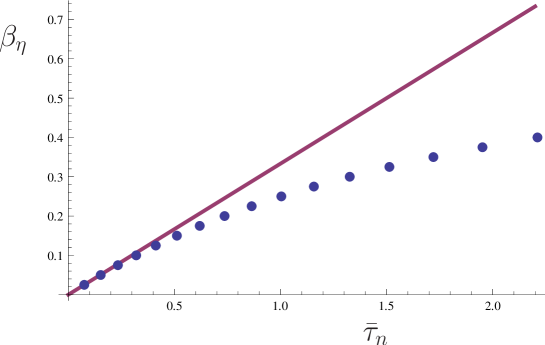
Figure 2: This figure shows the relation between the relaxation time in kinetic theory and the shear viscosity. We plot the dimensionless relaxation time $\bar{\tau}$ against the dimensionless shear viscosity $\beta_{\eta}$ defined in the text. The points were obtained by first solving the Navier-Stokes equation with a given values of $\beta_{\eta}$ for a trapped cloud with initial aspect ratio $A_{R}(0)=0.035$, and then determining the value of $\bar{\tau}$ that leads to the best fit of the solution of the Boltzmann equation to the Navier-Stokes result for $A_{R}(t)$ in the regime $t<1400$ ms. The line show the leading order relation $\beta_{\eta}=\bar{\tau}/3$. Note that the long dashed line in Fig. 1 corresponds to $\beta_{\eta}=0.25$.

This issue is studied in more detail in Fig. 2. For a given value of the viscosity coefficient $\alpha_{n}$ we determine the Navier-Stokes evolution and then fit the relaxation time coefficient $\tau_{n}$ in the kinetic calculation to provide the best fit to hydrodynamics. The figure shows the dimensionless parameter

$$\beta_{\eta}=\frac{\alpha_{n}}{(3N\lambda)^{1/3}}\frac{1}{E_{0}/E_{F}}\,$$ (15)

that governs the hydrodynamic evolution as a function of the dimensionless relaxation time

$$\bar{\tau}_{n}=\frac{\omega_{\perp}\tau_{n}}{T_{0}}\,.$$ (16)

In the hydrodynamic limit equ. (14) implies $\beta_{\eta}=\bar{\tau}_{n}/3$. This equation is satisfied at small $\tau_{n}$, but for $\bar{\tau}_{n}\mathrel{\hbox to0.0pt{\lower 4.0pt\hbox{\hskip 1.0pt$\sim$}\hss}\raise 1.0pt\hbox{$>$}}1$ the effective shear viscosity is smaller than the one predicted by the linear approximation. The fit in Fig. 1 corresponds to $\bar{\tau}_{n}=0.78$, which is close to the regime where higher order effects become large. Qualitatively, the behavior of $\beta_{\eta}$ as a function of $\bar{\tau}_{n}$ is easy to understand. At moderate $\tau_{n}$ the relaxation time approximation implies that the dissipative stress tensor equ. (12) does not reach the hydrodynamic limit equ. (13) instantaneously, but over a characteristic time $\tau_{n}/T_{\it le}$. For an expanding system this means that the time integral of the dissipative stresses in the kinetic theory is smaller as compared to the hydrodynamic limit. At large $\tau_{n}$ the solution of the Boltzmann equation approaches the ballistic limit, and dissipative effects saturate as $\bar{\tau}_{n}\to\infty$.

III Mean field effects

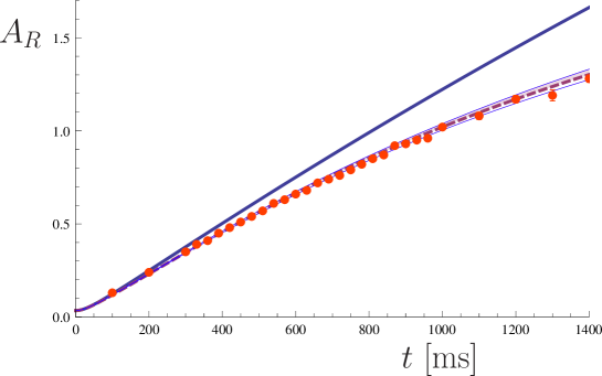
Figure 3: This figure shows the effect of the mean field potential on the evolution of the aspect ratio $A_{R}(t)$. The solid line shows the result in ideal hydrodynamics, and the points are experimental data from Cao:2010 taken at an initial energy $E/E_{F}=3.61$. The short dashed line is the result of a relaxation time fit to the data without mean field effects. The band around the dashed line shows the variation of $A_{R}(t)$ when mean field effects included. The upper and lower limits of the band correspond to $\xi=\pm 0.1$, respectively.

In this section we investigate possible mean field effects in the Boltzmann equation, in particular the question to what extent these effects cause uncertainties in the extraction of the relaxation time. Without mean field effects the equation of state is $P=nT$ and the relation between energy density and pressure is ${\cal E}=\frac{3}{2}P$. In the unitary gas scale invariance restricts the equation of state to be of the form $P=nTh(y)$ with $y=mT/n^{2/3}$ and $h(y)$ is a universal function which approaches unity in the high temperature, low density limit. The relation ${\cal E}=\frac{3}{2}P$ is exact irrespective of the functional form of $h(y)$. Scale invariance restricts the form of the mean field potential to be $U_{mf}=g(y)n(x)^{\alpha}$ with $\alpha=2/3$. For simplicity we will assume that $g(y)\sim{\it const}$. The mean field potential does not modify the equation for $\theta_{j}$. The equation for $b_{j}$ becomes

$$\ddot{b}_{j}+\omega_{j}^{2}b_{j}-\omega_{j}^{2}\frac{\theta_{j}}{b_{j}}+\omega_{j}^{2}\xi\left(\frac{\theta_{j}}{b_{j}}-\frac{1}{b_{j}{\cal V}^{\alpha}}\right)=0\,.$$ (17)

with ${\cal V}=\prod_{j}b_{j}$. The parameter $\xi$ is defined by

$$\xi=\frac{\langle U_{mf}\rangle}{\frac{1+\alpha}{3\alpha}m\langle v^{2}\rangle+\langle U_{mf}\rangle}\,.$$ (18)

In the limit of ideal hydrodynamics ($\tau\to 0$) we have $\theta_{j}=\bar{\theta}={\cal V}^{-2/3}$. This implies that mean field effects do not modify the evolution a scale invariant, non-dissipative gas. This result is known from studies of the unitary gas in the context of ideal hydrodynamics Schaefer:2009px ; Schafer:2010dv . The basic observation is that the Euler equation only depends on the relation $P({\cal E})$, and not on the equation of state $P(n,T)$.

For a finite relaxation time the relation $\theta_{j}={\cal V}^{-2/3}$ is only approximately satisfied and mean field corrections play a role. In order to estimate the size of mean field effects we relate the parameter $\xi$ to thermodynamic properties of the unitary gas. The static Boltzmann-Vlasov equation (5) implies

$$\frac{1}{2}m\langle v^{2}\rangle+\frac{3}{2}\frac{\alpha}{1+\alpha}\langle U_{mf}\rangle=\frac{m}{2}\sum_{i}\omega_{i}^{2}\langle r_{i}^{2}\rangle\,.$$ (19)

For a scale invariant gas with $\alpha=2/3$ the LHS of this relation is equal to the internal energy of the gas. Equ. (19) is then the well-known Virial theorem Thomas:2005 ; Werner:2006 ; Son:2007 : The total internal energy of a harmonically trapped system is equal to the potential energy. We can use equ. (19) to express $\xi$ in terms of the total energy of the gas. For $\alpha=2/3$ and in the limit $\xi\ll 1$ we find

$$\xi=\frac{E_{0}}{3NT}-1\,.$$ (20)

For an ideal gas the total (internal plus potential) energy is $E_{0}=3NT$ and $\xi=0$. We have computed $\xi$ using the equation of state described in the appendix of Schafer:2010dv . This equation of state is a parameterization of the recent experimental results of Nascimbene et al. Chevy:2009 . We find that in the normal fluid regime $|\xi|<0.1$, where $\xi<0$ at high temperature regime and $\xi>0$ near the critical temperature $T_{c}$. We note that at unitarity corrections to the equation of state due to quantum statistics are parametrically of the same order as mean field corrections. At high temperature quantum corrections are numerically small, but near $T_{c}$ equ. (20) is not reliable.

In Fig. 3 we show the effect of mean field corrections in the regime $-0.1\leq\xi\leq 0.1$ on the evolution of the system. Positive values of $\xi$ tend to push the evolution closer to the solution in ideal hydrodynamics, and therefore act like an effective negative viscosity. Negative values of $\xi$ act an effective positive shear viscosity. Fig. 3 shows that mean field effects are small compared to dissipative effects. We can quantify this observation using the data at $E/E_{F}=3.61$. A fit of the relaxation time using the Boltzmann equation without mean field effects gives $\bar{\tau}_{n}=1.14$. For this energy the equation of state described in Schafer:2010dv gives $\xi=-0.014$. If we refit the relaxation time using the Boltzmann-Vlasov equation with this value of $\xi$ we find $\bar{\tau}_{n}=1.12$, which is a $\sim 2\%$ correction.

IV Freezeout

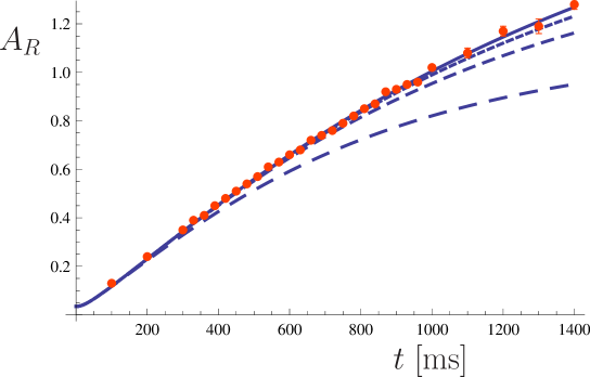
Figure 4: This figure shows the effect of freezeout on the time evolution of the aspect ratio. The data points show the results of Cao et al. also shown in Figs. 1 and 3. The solid line is the relaxation time fit shown in Fig. 3. The dashed lines show the same fit but with the scaling of the relaxation time changed from $\tau\sim 1/T$ to $\tau\sim T^{1/2}{\cal V}$ at a freezeout scale factor $b_{\it fr}=10,5,1$ (from top to bottom).

Up to this point we have considered a relaxation time of the form $\tau=\tau_{n}/T$ with $\tau_{n}={\it const}$. In this case the relaxation time scales as $\tau\sim\theta^{-1}\sim{\cal V}^{2/3}$. The expansion time, on the other hand, scales as $\tau\sim{\cal V}^{1/2}$ (at very late time the expansion changes from being two-dimensional to three-dimensional and $\tau\sim{\cal V}^{1/3}$). This implies that the system will eventually freeze out, and the nature of the expansion will change from hydrodynamic to ballistic. We note, however, that for the values of $\tau_{n}$ that fit the data shown in Fig. 1,3 freezeout occurs late, for $A_{R}>1$. At this time the density has dropped by a factor of order $\lambda^{-2}\sim 10^{3}$.

To maintain hydrodynamic behavior despite the large drop in density requires the system to be very close to the unitary limit. At unitarity the mean free path scales as $l_{\it mfp}\sim(n\sigma)^{-1}\sim{\cal V}\lambda_{\it deB}^{-2}\sim{\cal V}^{1/3}$, where $\lambda_{\it deB}\sim(mT)^{-1/2}$ is the thermal wave length. This implies that the the mean free path grows more slowly as the system size. For a weakly collisional system, on the other hand, we have $l_{\it mfp}\sim(na^{2})^{-1}\sim{\cal V}$ and the mean free path grows more quickly than the system size.

In this section we wish to check whether the data support the idea that freezeout occurs late. For this purpose we impose a freezeout time $t_{\it fr}$ so that for $t<t_{\it fr}$ the relaxation time scales as $\tau\sim\tau_{n}/T$ and for $t>t_{\it fr}$ the relaxation time scales as $\tau\sim\gamma{\cal V}/T^{1/2}$, which is the behavior expected for a constant cross section $\sigma\sim a^{2}$. The parameter $\tau_{n}$ is taken from the previous fit and $\gamma$ is adjusted so that $\tau$ is continuous at $t=t_{\it fr}$. In Fig. 4 we show the evolution of the aspect ratio $A_{R}(t)$ for different choices of the freezeout time. The solid line shows the result for $t_{\it fr}\to\infty$, and the dashed curves correspond to freezeout scale parameters $b_{\perp}(t_{\it fr})=10,5,1$. We observe that $t_{\it fr}\to\infty$ provides the best fit to the data, and $b_{\perp}(t_{\it fr})\mathrel{\hbox to0.0pt{\lower 4.0pt\hbox{\hskip 1.0pt$\sim$}\hss}\raise 1.0pt\hbox{$<$}}5$ is clearly excluded. We conclude that for the conditions explored experimentally ($N\sim 2\cdot 10^{5}$ and $E/E_{F}\leq 3.61$) the density can drop by a least a factor $\sim 25$ before freezeout occurs.

V High temperature limit of the relaxation time

In the high temperature limit the viscous relaxation time can be computed reliably. The result is $\tau=\eta/(nT)$ with $\eta=\eta_{0}(mT)^{3/2}$ and $\eta_{0}=15/(32\sqrt{\pi})$ Bruun:2005 ; Bruun:2006 ; Chao:2010tk . This implies that even within the relaxation time approximation the collision term is a nonlinear functional of the distribution function. We have

$$C[f]=-\frac{T_{\it le}}{\eta_{0}(mT_{\it le})^{3/2}}\left[\int d^{3}\bar{v}\,f(x,{\bar{v}},t)\right]\left(f(x,v,t)-f_{\it le}(x,v,t)\right)\,.$$ (21)

We note that even in the simplest case $1/\tau\sim T_{\it le}/\tau_{n}$ with $\tau_{n}={\it const}$ the relaxation time is a functional (via the temperature) of the distribution function. However, for the scaling ansatz in equ. (3) the temperature is only a function of time. The collision term in equ. (21) is more complicated because the relaxation time is a function of time and position (but not of velocity). This means that it is difficult to find exact solutions of the Boltzmann equation. We obtain an approximate scaling solution by using the same ansatz for $f(x,v,t)$ as before. The parameters $b_{i}$ and $\theta_{i}$ are again fixed by taking moments of the Boltzmann equation weighted with $R_{i}^{2},U_{i}^{2}$ and $R_{i}U_{i}$. We find that only the $U_{i}^{2}$ equation is modified. As a consequence equ. (7) is replaced by

$$\dot{\theta}_{j}+2\frac{\dot{b}_{j}}{b_{j}}\theta_{j}=-\frac{\langle n_{0}\rangle\bar{\theta}}{\eta_{0}(m\bar{\theta})^{3/2}{\cal V}}\left(\theta_{j}-\bar{\theta}\right)\,,$$ (22)

where $\langle n_{0}\rangle=\int d^{3}r\,n_{0}(r)^{2}/\int d^{3}rn_{0}(r)$ is the average density in the initial state. Note that for a Gaussian distribution $\langle n_{0}\rangle=2^{-3/2}n_{0}(0)$. We also observe that to leading order in $\tau$ the parameter $\bar{\theta}$ evolves as $\bar{\theta}={\cal V}^{-2/3}$. This implies that the RHS of equ. (22) scales as $T_{0}\bar{\theta}/\tau_{n}$ with $\tau_{n}=\eta_{0}(mT_{0})^{3/2}/\langle n_{0}\rangle$. As a consequence, the evolution of the system in the Navier-Stokes regime (that is to first order in $\tau$) is indistinguishable from the result shown in Fig. 1. What is new is the explicit relation between $\tau_{n}$ and the shear viscosity in the high temperature, low density limit.

This relation can be compared to the analysis presented by Cao et al. in Cao:2010 . In this work the authors attempted to extract $\eta_{0}$ from experimental data on elliptic flow in the high temperature regime using the Navier-Stokes equation. The problem with the Navier-Stokes analysis is that a density independent shear viscosity leads to an infinitely large dissipative contribution from the dilute corona. Cao et al. argued that a correct treatment of the corona has to take into account the fact that at low density the dissipative stress tensor cannot instantaneously relax to the Navier-Stokes form. They proposed that this effect can be taken into account by using a simple model for the viscosity which is of the form $\eta(x)=\eta_{0}(mT)^{3/2}(n(x)/n(0))$. A more detailed justification for this model can be found in Schaefer:2009px . The model of Cao et al. can be written as $\eta=\alpha_{n}n$ with $\alpha_{n}=\eta_{0}(mT)^{3/2}/n(0)$. Because the temperature drops (approximately) as $T\sim n(0)^{2/3}$ this corresponds to a constant value of $\alpha_{n}=\eta_{0}(mT_{0})^{3/2}/n_{0}(0)$. This equation for $\alpha_{n}$ has the same structure as the result that follows from equ. (22), but it differs by the numerical factor $\langle n_{0}\rangle/n_{0}(0)$. This difference is clearly very significant, and it represents the most important uncertainty in the extraction of $\eta_{0}$ from data. This uncertainty can only be addressed by studying more accurate solution of the Boltzmann equation in the case of a density dependent relaxation time.

VI Bulk viscosity

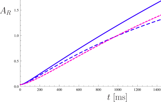
Figure 5: This figure shows the effect of shear and bulk viscosity on the evolution of the aspect ratio $A_{R}(t)$ in viscous hydrodynamics. The solid line shows the result in ideal hydrodynamics, the long dashed line corresponds to the Navier-Stokes equation with $\beta_{\eta}=0.25$, and the short dashed line shows the Navier-Stokes result for $\beta_{\zeta}=0.25$. The system parameters are the same as in Fig. 1.

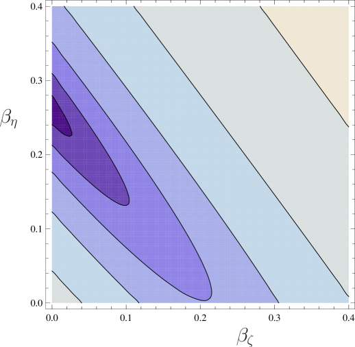
Figure 6: This figure shows $\log(\chi^{2})$ contours for a hydrodynamic fit to the data of Cao et al. shown in Fig. 1. The minimum of $\chi^{2}$ corresponds to the dark region. The two parameter $\beta_{\zeta}$ and $\beta_{\eta}$ control the bulk and shear viscosity of the system.

Finally, we wish to study the possible effects of bulk viscosity on the evolution of the cloud. At unitarity we expect the bulk viscosity to vanish Son:2005tj . There are nevertheless at least two reasons for studying dissipative effects associated with bulk motion. The first is to verify that the theoretical prediction $\zeta=0$ at unitarity is indeed correct. The second is to understand how bulk viscosity manifests itself as one moves away from unitarity.

In Sect. II we showed that the relaxation time approximation to the Boltzmann equation (without mean field effects) leads to a traceless dissipative stress tensor, see equ. (12,13). We can break scale invariance by using a mean field potential with $\alpha\neq 2/3$. However, within the approximations used in Sect. III, scale breaking in the Boltzmann-Vlasov equation does not lead to a trace-term in the dissipative stress tensor. We will therefore study the role of bulk viscosity using the Navier-Stokes equation. We will follow Cao:2010 ; Schafer:2010dv and use a scaling ansatz for the hydrodynamic variables,

$$n(x_{i},t)={\cal V}^{-1}n_{0}(x_{i}/b_{i},t)\,,\hskip 28.45274ptV_{i}=(\dot{b}_{i}/b_{i})x_{i}\,,\hskip 28.45274pt(\nabla_{i}P)/n=a_{i}x_{i}\,.$$ (23)

The functional form of the density $n$ and the velocity field $V_{i}$ agree with the results obtained in Sect. II. In the Navier-Stokes limit the function $a_{i}(t)$ can be related to the parameter $\theta_{i}(t)$ in the distribution function by $a_{i}=\theta_{i}\omega_{i}^{2}/b_{i}^{2}$. For an axially symmetric system the equations of motion for $b_{i}$ and $a_{i}$ are given by

$$\frac{\ddot{b}_{\perp}}{b_{\perp}} = a_{\perp}-\frac{2\beta_{\eta}\omega_{\perp}}{b^{2}_{\perp}}\left(\frac{\dot{b}_{\perp}}{b_{\perp}}-\frac{\dot{b}_{z}}{b_{z}}\right)-\frac{3\beta_{\zeta}\omega_{\perp}}{b^{2}_{\perp}}\left(2\frac{\dot{b}_{\perp}}{b_{\perp}}+\frac{\dot{b}_{z}}{b_{z}}\right)\,,$$ (24)

$$\frac{\ddot{b}_{z}}{b_{z}} = a_{z}+\frac{4\beta_{\eta}\lambda\omega_{z}}{b^{2}_{z}}\left(\frac{\dot{b}_{\perp}}{b_{\perp}}-\frac{\dot{b}_{z}}{b_{z}}\right)-\frac{3\beta_{\zeta}\lambda\omega_{z}}{b^{2}_{z}}\left(2\frac{\dot{b}_{\perp}}{b_{\perp}}+\frac{\dot{b}_{z}}{b_{z}}\right)\,,$$ (25)

$$\dot{a}_{\perp} = \mbox{}-\frac{2}{3}\,a_{\perp}\left(5\,\frac{\dot{b}_{\perp}}{b_{\perp}}+\frac{\dot{b}_{z}}{b_{z}}\right)+\frac{8\beta_{\eta}\omega_{\perp}^{2}}{3b^{2}_{\perp}}\left(\frac{\dot{b}_{\perp}}{b_{\perp}}-\frac{\dot{b}_{z}}{b_{z}}\right)^{2}+\frac{2\beta_{\zeta}\omega_{\perp}^{2}}{b^{2}_{\perp}}\left(2\frac{\dot{b}_{\perp}}{b_{\perp}}+\frac{\dot{b}_{z}}{b_{z}}\right)^{2}\,,$$ (26)

$$\dot{a}_{z} = \mbox{}-\frac{2}{3}\,a_{z}\left(4\,\frac{\dot{b}_{z}}{b_{z}}+2\,\frac{\dot{b}_{\perp}}{b_{\perp}}\right)+\frac{8\beta_{\eta}\lambda\omega_{z}}{3b_{z}^{2}}\left(\frac{\dot{b}_{\perp}}{b_{\perp}}-\frac{\dot{b}_{z}}{b_{z}}\right)^{2}+\frac{2\beta_{\zeta}\lambda\omega_{z}}{b_{z}^{2}}\left(2\frac{\dot{b}_{\perp}}{b_{\perp}}+\frac{\dot{b}_{z}}{b_{z}}\right)^{2}\,.$$ (27)

Here, $\beta_{\eta}$ is defined in equ. (15) and $\beta_{\zeta}$ is the analogous parameter that controls the effect of bulk viscosity

$$\beta_{\zeta}=\frac{\zeta_{n}}{(3N\lambda)^{1/3}}\frac{1}{E_{0}/E_{F}}\,$$ (28)

with $\zeta=\zeta_{n}n$. For $\beta_{\zeta}=0$ and to first order in $\beta_{\eta}$ eqns. (24-27) are equivalent to eqns. (6,7). Solutions of these equations for $(\beta_{\eta},\beta_{\zeta})=(0.25,0)$ and $(\beta_{\eta},\beta_{\zeta})=(0,0.25)$ are shown in Fig. 5. We see that the effects of shear and bulk viscosity are clearly distinguishable. Shear viscosity leads to a characteristic curvature in the time dependence of the aspect ratio. This is related to the fact that shear viscosity is more efficient in moving kinetic energy from transverse motion to longitudinal motion, combined with the fact that the longitudinal expansion takes place on a longer time scale. A comparison with the data of Cao et al. is shown in Fig. 6. The figure shows $\chi^{2}$ contours for a fit to the data at $E/E_{f}=3.61$ using both $\beta_{\eta}$ and $\beta_{\zeta}$ as fit parameters. We observe that the absolute minimum is at $\beta_{\eta}=0.25$ and $\beta_{\zeta}=0.0$ ($\alpha_{n}=22.1$ and $\zeta_{n}=0.0$). We conclude that the data at unitarity favor a vanishing bulk viscosity and a non-zero shear viscosity.

VII Summary and conclusions

In this paper we have studied a number of issues related to the crossover between kinetic theory and hydrodynamics. In this section we briefly summarize the main findings and point to open problems.

1. Dimensional analysis implies that the shear viscosity and the relaxation time can be written as $\eta=\alpha_{n}n$ and $\tau=\tau_{n}/T$, respectively. Scale invariance dictates that at unitarity $\alpha_{n}$ and $\tau_{n}$ are only functions of $y=mT/n^{2/3}$. The matching between kinetic theory in the relaxation time approximation and hydrodynamics is simplest in the case that $\alpha_{n}$ and $\tau_{n}$ are constant. In this case the matching condition is simply $\alpha_{n}=\tau_{n}$, and we showed that for systems that have been studied experimentally terms of higher order in $\tau$ are not large.

2. The Boltzmann equation describes the evolution of a system that obeys an ideal gas equation of state, $P=nT$. Corrections due to a more complicated equation of state can be taken into account using the Boltzmann-Vlasov equation and a mean field potential. At unitarity and in the limit $\tau\to 0$ the mean field potential has no effect on the evolution of the system. As a consequence, mean field corrections remain small even if the relaxation time is not zero. Using the mean energy per particle from a realistic equation of state we find that the uncertainty in the shear viscosity related to mean field effects is $\sim 2\%$. This is consistent with the effect due to the deviation of the equation of state from $P=nT$ found in calculations using the Navier-Stokes equation Schafer:2010dv .

3. We also studied the effect of a possible freezeout, that means a transition from hydrodynamic to ballistic behavior, on the evolution of the system. Freezeout could occur because the scattering length is not strictly infinite, or because non-equilibrium effects not captured by the Boltzmann equation cause the growth of the transport cross section to lag behind the equilibrium prediction. We showed that the experimental data obtained by Cao et al. Cao:2010 require that freezeout has to occur late, for values of the scale parameters $b_{\perp}\mathrel{\hbox to0.0pt{\lower 4.0pt\hbox{\hskip 1.0pt$\sim$}\hss}\raise 1.0pt\hbox{$>$}}5$. This implies that the unitary Fermi gas remains hydrodynamic despite the fact that the density drops significantly during the expansion.

4. Finally, we studied the possible role of bulk viscosity on the evolution of the system. We showed that there are characteristic differences between dissipative effects due to bulk and shear viscosity, and that the data are best described by shear viscosity only.

There are a number of issues that remain to be resolved. We have studied the Boltzmann equation with a relaxation time that scales as $\tau\sim T^{1/2}/n$. This is the scaling which is predicted by the linearized form of the full collision terms using the scattering amplitude in the unitary limit. It corresponds to a shear viscosity that is only a function of temperature and not of density. For simplicity we have employed the scaling ansatz equ. (3) for the distribution function and solved for the coefficients by taking moments. We obtain an equation of motion which is equivalent to the case $\tau=\tau_{n}/T$ with an effective $\tau_{n}=\eta(T_{0})/\langle n_{0}\rangle$. This result is in qualitative, but not in quantitative, agreement with an estimate based on hydrodynamics with a finite relaxation time Schaefer:2009px ; Cao:2010 . In order to resolve this disagreement we need to find more accurate solutions of the Boltzmann equation. For infinite systems there are solutions to the linearized Boltzmann equation that can be matched to second order hydrodynamics Chao:2010tk , but the corresponding solutions for an expanding system have not been determined.

We also observed that within the approximations used in this work the Boltzmann equation does not account for bulk viscosity even if scale invariance is broken by mean field corrections to the equation of state. It is known that the integral of the frequency dependent bulk viscosity is non-zero if the equation of state violates scale invariance Taylor:2010ju . It is not know what the leading $1/a$ term in the bulk viscosity is, and what terms in the Boltzmann equation have to be kept in order to reproduce this term.

Acknowledgments: This work was supported in parts by the US Department of Energy grant DE-FG02-03ER41260. We thank John Thomas for useful discussions.

References

- (1) I. Bloch, J. Dalibard, W Zwerger, Rev. Mod. Phys. 80, 885 (2008) [arXiv:0704.2511].
- (2) S. Giorgini, L. P. Pitaevskii, S. Stringari, Rev. Mod. Phys. 80 1215 (2008) [arXiv:0706.3360].
- (3) C. Chin, R. Grimm, P. Julienne, E. Tiesinga Rev. Mod. Phys. 82 1225 (2010) [arXiv:0812.1496].
- (4) T. Schäfer and D. Teaney, Rept. Prog. Phys. 72, 126001 (2009) [arXiv:0904.3107 [hep-ph]].
- (5) K. M. O’Hara, S. L. Hemmer, M. E. Gehm, S. R. Granade, J. E. Thomas, Science Vol. 298, No. 5601, 2179 (2002) [cond-mat/0212463].
- (6) T. Schäfer, Phys. Rev. A 76, 063618 (2007) [arXiv:cond-mat/0701251].
- (7) A. Turlapov, J. Kinast, B. Clancy, L. Luo, J. Joseph, J. E. Thomas, J. Low Temp. Phys. 150, 567 (2008) [arXiv:0707.2574].
- (8) T. Schäfer and C. Chafin, arXiv:0912.4236 [cond-mat.quant-gas].
- (9) J. E. Thomas, Nucl. Phys. A 830, 665C (2009).
- (10) C. Cao, E. Elliott, J. Joseph, H. Wu, J. Petricka, T. Schäfer, J. E. Thomas, arXiv:1007.2625 [cond-mat.quant-gas].
- (11) P. Kovtun, D. T. Son and A. O. Starinets, Phys. Rev. Lett. 94, 111601 (2005) [arXiv:hep-th/0405231].
- (12) I. Arsenne et al. [Brahms], B. Back et al. [Phobos], K. Adcox et al. [Phenix], J. Adams et al. [Star], “First Three Years of Operation of RHIC”, Nucl. Phys. A757, 1-183 (2005).
- (13) P. Romatschke and U. Romatschke, Phys. Rev. Lett. 99, 172301 (2007) [arXiv:0706.1522 [nucl-th]].
- (14) K. Dusling and D. Teaney, Phys. Rev. C 77, 034905 (2008) [arXiv:0710.5932 [nucl-th]].
- (15) H. Song and U. W. Heinz, arXiv:0812.4274 [nucl-th].
- (16) D. Guery-Odelin, F. Zambelli, J. Dalibard, and S. Stringari, Phys. Rev. A 60 4851 (1999).
- (17) P. Pedri, D. Guery-Odelin and S. Stringari, Phys. Rev. A 68 043608 (2003) [ond-mat/0305624]
- (18) D. Guery-Odelin, Phys. Rev. A 66 033613 (2002).
- (19) C. Menotti, P. Pedri, S. Stringari, Phys. Rev. Lett. 89, 250402 (2002) [cond-mat/0208150].
- (20) B. Jackson, P. Pedri, and S. Stringari, Europhys. Lett. 67 524 (2004).
- (21) T. Nikuni, A. Griffin Phys. Rev. A 69, 023604 (2004) [arXiv:cond-mat/0309269].
- (22) G. M. Bruun, H. Smith, Phys. Rev. A 72, 043605 (2005) [cond-mat/0504734].
- (23) G. M. Bruun, H. Smith, Phys. Rev. A 75, 043612 (2007) [cond-mat/0612460].
- (24) G. M. Bruun, H. Smith Phys. Rev. A 76, 045602 (2007) [arXiv:0709.1617].
- (25) D. T. Son, Phys. Rev. Lett. 98, 020604 (2007) [arXiv:cond-mat/0511721].
- (26) T. Enss, R. Haussmann, W. Zwerger, Annals Phys. 326, 770-796 (2011). [arXiv:1008.0007 [cond-mat.quant-gas]].
- (27) T. Schäfer, Phys. Rev. A (2010), in press [arXiv:1008.3876 [cond-mat.quant-gas]].
- (28) J. E. Thomas, J. Kinast, and A. Turlapov, Phys. Rev. Lett. 95, 120402 (2005) [arXiv:cond-mat/0503620].
- (29) F. Werner and Y. Castin, Phys. Rev. A 74, 053604 (2006) [cond-mat/0607821].
- (30) D. T. Son, arXiv:0707.1851.[cond-mat.other].
- (31) S. Nascimbene, N. Navon, K. Jiang, F. Chevy, C Salomon, Nature 463, 1057 (2010) [arXiv:0911.0747[cond-mat.quant-gas]].
- (32) J. Chao, M. Braby, T. Schäfer, [arXiv:1012.0219 [cond-mat.quant-gas]].
- (33) E. Taylor and M. Randeria, Phys. Rev. A81, 053610 (2010). [arXiv:1002.0869 [cond-mat.quant-gas]].