A Generic Multivariate Distribution for Counting Data

Abstract

Motivated by the need, in some Bayesian likelihood free inference problems, of imputing a multivariate counting distribution based on its vector of means and variance-covariance matrix, we define a generic multivariate discrete distribution. Based on blending the Binomial, Poisson and Negative-Binomial distributions, and using a normal multivariate copula, the required distribution is defined. This distribution tends to the Multivariate Normal for large counts and has an approximate pmf version that is quite simple to evaluate.

KEYWORDS: Counting Data; Bayesian inference in epidemics; Copulas.

1 Introduction

We develop a generic discrete multivariate distribution defined in terms of its mean and covariate matrix only. The multivariate Normal distribution is defined in such terms and would be the default option as an inputed distributions when only the mean and covariance matrix are available for an otherwise unknown distribution. However, there is no alternative when considering discrete data, specially in the case of low counts where a Normal approximation is not feasible. The motivation to defining such discrete distribution is as follows.

The development and analysis of mathematical epidemic models that take into account uncertainty is an active field of research (Bretó et al., 2009; Alonso et al., 2007; Finkenstadt et al., 2002; Schwartz et al., 2004; Nåsell, 2002; Chen and Bokka, 2005; Andersson and Britton, 2000). The importance of this field of research is apparent given its potential impact on public health policies to handle emergent and re-emergent infectious diseases such as dengue fever, Lyme disease, tuberculosis, flu, etc. It is known that the effects of local (demographic) stochasticity weight more in determining the dynamics of epidemics when the number of individuals in the population is low. On the other hand, parameter estimation is among the standard tools to explore the predictive capacity of models from partial observation of the state variables. In this context, it is specially important to devise methods to study the predictive capacity of the mathematical models, in particular, to quantify the uncertainties.

For the sake of clarity we use the simplest epidemic model, e.g. the SIR model without vital dynamics. Let the random variables $X_{1}$, $X_{2}$ and $X_{3}$ denote the number of Susceptible, Infected and Recovered individuals in a closed population at a given time $t$, respectively. The stochastic model is defined by the processes through which it evolves:

$$X_{1}+X_{2} \stackrel{{\scriptstyle b_{0}\frac{X_{2}}{\Omega}}}{{\longrightarrow}}2X_{2}$$

$$X_{2} \stackrel{{\scriptstyle b_{1}}}{{\longrightarrow}}X_{3}$$

If we denote by $x_{1}$, $x_{2}$ and $x_{3}$ a realization of the random variables $X_{1}$, $X_{2}$ and $X_{3}$, and let $P_{\bar{x}}(t)=P(x_{1},x_{2},x_{3},t)$ be the probability that the system is in state $(x_{1},x_{2},x_{3})$ at time $t$, then the chemical master equation (van Kampen, 1992) for this system is given by

$$\begin{split}\frac{dP(x_{1},x_{2},x_{3},t)}{dt}=&b_{0}\frac{(x_{1}+1)}{\Omega}(x_{2}-1)P(x_{1}+1,x_{2}-1,x_{3},t)\\ &+b_{1}(x_{2}+1)P(x_{1}+1,x_{2}-1,x_{3}-1,t)\\ &-(b_{0}\frac{x_{1}}{\Omega}x_{2}+b_{1}x_{2})P(x_{1},x_{2},x_{3},t),\end{split}$$ (1)

where the constant $\Omega$ denotes the total number of individuals, and $b_{0}$ and $b_{1}$ are respectively the contact rate and the rate of loss of infectiousness.

Applying the Inverse Size Expansion (van Kampen, 1992) to equation 1 leads to equations for the expected value and the fluctuations of $x_{1}$, $x_{2}$ and $x_{3}$. The Fokker-Plank approximation is then used leading to an approximation for the mean $E_{t}(X_{i})$ and cross products $E_{t}(X_{i}X_{j})$ for all species $i,j=1,2,\ldots,k$ at each time $t$ Chen and Bokka (2005). As far as the distribution for the $X_{j}$’s is concern we know to be dealing with counting data $X_{i}\in\mathbb{N};i=1,2,\ldots,k$ and, for a fixed time $t$, we have (an approximation for) their means $\mu_{i}=E_{t}(X_{i})$, variances $v_{i}=E_{t}(X_{i}^{2})-\mu_{i}^{2}$ and their correlations $\rho_{ij}=\frac{E_{t}(X_{i}X_{j})-\mu_{i}\mu_{j}}{\sqrt{v_{i}v_{j}}}$.

It is possible to simulate directly from the true model $P(\cdot,t)$ above (for fixed $b_{0}$ and $b_{1}$) to simulate realizations of $(X_{1}(t),X_{2}(t),X_{3}(t))$ (Gillespie, 2007). Data is commonly only available for $X_{2}(t)$ and for specific epidemics (eg. Dengue fiver) there is substantial prior expert information for the contact rate, $b_{0}$, and the rate of loss of infectiousness, $b_{1}$. It would be possible to use the ABC algorithm (Marin et al., 2011) to make Bayesian inferences about $b_{0}$ and $b_{1}$ but the simulation procedure becomes very slow for moderate population sizes $\Omega$ and still the ABC approach lacks a formal theoretical foundation (Marin et al., 2011, p. 4). Instead, using the moment approximation explained above (that indeed depends on the parameters of interest $b_{0}$ and $b_{1}$), we impute a counting (discrete) distribution on the observables (commonly $X_{2}(t)$ but in some situations all $X_{1}(t),X_{2}(t),X_{3}(t)$ are observed unknonw, 1978) matching those moments to create a likelihood. The computational complexity of this likelihood is in fact independent of $\Omega$ and, using elicited priors and MCMC, a Bayesian inference is possible for any set of population sizes. We have had already promising results along these lines and will publish such research in an specialized journal of the field.

We will assume that the correlation matrix $\boldsymbol{\rho}=(\rho_{ij})$ is positively defined and, certainly, $\mu_{i},v_{i}>0$. Based on this information only, we need to impute a discrete distribution for the observables $(X_{1},X_{2},X_{3})$ that would be defined by these moments. Here we propose such generic multivariate distribution for counting data. In the next section we explain the univariate version, which is a simple combination of the default distributions commonly used for counting data, namely, the Binomial, the Poisson and the Negative Binomial. In Section 3 we create the multivariate version using a Normal copula and in Section 4 present some examples.

2 A Univariate Generic Discrete Distribution $Gd(m,v)$

The Poisson, Binomial and Negative Binomial distributions are simple form distributions and first candidates for counting data models. For any mean and variance $\mu,v>0$ we make a combination of these three distributions in the following way

$$Gd(x|\mu,v)=\begin{cases}C_{x}^{m}\leavevmode\nobreak\ p^{x}(1-p)^{m-x};\leavevmode\nobreak\ x=0,1,\ldots m&\text{if}\leavevmode\nobreak\ \leavevmode\nobreak\ \mu>v\\ e^{-v}\frac{v^{x}}{x!};\leavevmode\nobreak\ x\in\mathbb{N}&\text{if}\leavevmode\nobreak\ \leavevmode\nobreak\ \mu=v\\ C_{x-1}^{x+m-1}\leavevmode\nobreak\ p^{x}(1-p)^{m};\leavevmode\nobreak\ x\in\mathbb{N}&\text{if}\leavevmode\nobreak\ \leavevmode\nobreak\ \mu<v\\ \end{cases}$$ (2)

where $p=1-\min\left\{\frac{m}{v},\frac{v}{m}\right\}$, $m=\frac{\mu^{2}}{|\mu-v|}$ and $C_{x}^{m}$ are the combinations of $m$ items taken in subsets of size $x$. That is, we use a Binomial if $\mu>v$, a Poisson if $\mu=v$ and a Negative-Binomial if $\mu<v$. Neither of these distributions can handle any mean and variance; by combining these distributions we obtain the Generic Discrete class $Gd(\mu,v)$ defined for arbitrary mean $\mu$ and variance $v$, $\mu,v>0$, and these two moments completely define the distribution.

Indeed, it is straightforward to see that if $X\sim Gd(\mu,v)$, $E(X)=\mu$ and $V(X)=v$. More importantly, for a fixed mean $\mu$, given both the properties of the Binomial and the Negative-Binomial, we see that

$$\lim_{v\rightarrow\mu}Gd(x|\mu,v)=e^{-v}\frac{v^{x}}{x!}.$$

Therefore we have a continuous evolution of this parametric class, being the Poisson the “continuous bridge” between the Binomial ($\mu>v$) and Negative Binomial ($\mu<v$). (Note that if $\mu>v$ and $v\rightarrow\mu$, the support will increase to cover all $\mathbb{N}$ since $m\rightarrow\infty$.)

Moreover, if $X\sim Gd(\mu,v)$, $\frac{X-\mu}{\sqrt{v}}$ will tend to a standard Normal distribution if $\mu\rightarrow\infty$ and $p\rightarrow p_{0}\in(0,1)$. That is, for large $\mu$ (and for example $\mu-3\sqrt{v}>0$) $Gd(\mu,v)$ can be approximated with a $N(\mu,v)$. Practical guidelines for approximating the Poisson, Binomial and Negative-Binomial distributions should be used when calculating the cdf, pmf etc. of $Gd(\mu,v)$. We then see that the $Gd(\mu,v)$ family evolves to a Normal distribution when $\mu$ is large (large counts).

3 The Multivariate Case

Suppose we have $k=2$ discrete distributions and we let $\boldsymbol{\mu}=(\mu_{1},\mu_{2})^{\prime}$ and $\boldsymbol{v}=(v_{1},v_{2})^{\prime}$ be their vector of means and variances and $\rho=\rho_{1,2}$. We require a bivariate discrete distribution, defined in terms of $\boldsymbol{\mu}$, $\boldsymbol{v}$ and $\rho$, such that the marginal distribution for each $X_{i}$ is $Gd(\mu_{i},v_{i})$ and the resulting correlation between $X_{1}$ and $X_{2}$ is (at least approximately) $\rho$.

We use a Normal Copula (see Nelsen, 2006, chap. 2) to create a a joint distribution. Let

$$\phi_{\rho}(s,t)=\frac{1}{2\pi\sqrt{1-\rho^{2}}}\exp\left\{-\frac{(s^{2}-2\rho st+t^{2})}{2(1-\rho^{2})}\right\}$$

be the bivariate standard normal distribution with correlation $\rho$ and $\Phi(s)$ the standard normal cdf. The normal Copula is defined as

$$C_{\rho}(u,v)=\int_{-\infty}^{\Phi^{-1}(u)}\int_{-\infty}^{\Phi^{-1}(v)}\phi_{\rho}(s,t)dsdt.$$

We define the joint cdf of $X_{1}$ and $X_{2}$ as

$$F_{\boldsymbol{\mu},\boldsymbol{v},\rho}(x_{1},x_{2})=C_{\rho}(F_{\mu_{1},v_{1}}(x_{1}),F_{\mu_{2},v_{2}}(x_{2})),$$

where $F_{\mu,v}$ is the cdf of a $Gd(\mu,v)$. $F_{\boldsymbol{\mu},\boldsymbol{v},\rho}(x_{1},x_{2})$ defines the Generic Discrete distribution in dimension 2, $Gd_{2}(\boldsymbol{\mu},\boldsymbol{v},\rho)$, and it is straightforward to verify that its pmf is

$$Gd_{2}(x_{1},x_{2}|\boldsymbol{\mu},\boldsymbol{v},\rho) = C_{\rho}(F_{\mu_{1},v_{1}}(x_{1}),F_{\mu_{2},v_{2}}(x_{2}))-C_{\rho}(F_{\mu_{1},v_{1}}(x_{1}-1),F_{\mu_{2},v_{2}}(x_{2}))-$$

$$C_{\rho}(F_{\mu_{1},v_{1}}(x_{1}),F_{\mu_{2},v_{2}}(x_{2}-1))+C_{\rho}(F_{\mu_{1},v_{1}}(x_{1}-1),F_{\mu_{2},v_{2}}(x_{2}-1))$$

(that is, the pmf are the corresponding jumps in the stepped cdf $F_{\boldsymbol{\mu},\boldsymbol{v},\rho}(x_{1},x_{2})$). Since $C_{\rho}(u,v)$ is a Copula for every $-1\leq\rho\leq 1$, the marginal distributions will be precisely $Gd(\mu_{1},v_{1})$ and $Gd(\mu_{2},v_{2})$, as required (Nelsen, 2006).

By pretending $F_{\mu_{i},v_{i}}(x_{i})$ is differentiable, with derivative $Gd(x_{i}|\mu_{i},v_{i})$, ‘differentiating’ $F_{\boldsymbol{\mu},\boldsymbol{v},\rho}(x_{1},x_{2})$ suggest the following approximation to the pmf

$$Gd_{2}(x_{1},x_{2}|\boldsymbol{\mu},\boldsymbol{v},\rho)\approx gd_{2}(x_{1},x_{2}|\boldsymbol{\mu},\boldsymbol{v},\rho)=K\frac{\phi_{\rho}(s,t)}{\phi(s)\phi(t)}Gd(x_{1}|\mu_{1},v_{1})Gd(x_{2}|\mu_{2},v_{2})$$ (4)

were $s=\Phi^{-1}(F_{\mu_{1},v_{1}}(x_{1}))$, $t=\Phi^{-1}(F_{\mu_{2},v_{2}}(x_{2}))$ and $\phi(\cdot)$ is the standard Normal pdf, for some normalization constant $K$. This approximation will prove useful even for $\mu_{i}$ small, and is far less computationally demanding than the exact version in (3).

If $F_{\mu_{i},v_{i}}(x_{i})$ were cdf’s of $N(\mu_{i},v_{i})$, that is $F_{\mu_{i},v_{i}}(x_{i})=\Phi\left(\frac{x_{i}-\mu_{i}}{\sqrt{v_{i}}}\right)$, we immediately see that the correlation between $X_{1}$ and $X_{2}$ is $\rho$. In the general case as each marginal distribution $Gd(\mu_{i},v_{i})$ becomes similar to a Normal distribution the actual correlation will be approximately $\rho$ and $Gd_{2}$ becomes increasingly similar to a Bivariate Normal distribution with the correct moments.

Finally, the multivariate generic discrete distribution is defined as

$$Gd_{n}(\boldsymbol{x}|\boldsymbol{\mu},\boldsymbol{v},\boldsymbol{\rho})=\int_{\Phi^{-1}(F_{\mu_{1},v_{1}}(x_{1}-1))}^{\Phi^{-1}(F_{\mu_{1},v_{1}}(x_{1}))}\cdots\int_{\Phi^{-1}(F_{\mu_{n},v_{n}}(x_{n}-1))}^{\Phi^{-1}(F_{\mu_{n},v_{n}}(x_{n}))}(2\pi)^{-n/2}|\boldsymbol{\rho}|^{-1/2}\exp\left\{-{1\over 2}\boldsymbol{s}^{\prime}\boldsymbol{\rho}^{-1}\boldsymbol{s}\right\}ds_{1}\cdots ds_{n}.$$

The corresponding approximate pmf would be

$$gd_{n}(\boldsymbol{x}|\boldsymbol{\mu},\boldsymbol{v},\boldsymbol{\rho})=K\frac{\phi_{\boldsymbol{\rho}}(s_{1},s_{2},\ldots,s_{n})}{\phi(s_{1})\phi(s_{2})\cdots\phi(s_{n})}Gd(x_{1}|\mu_{1},v_{1})Gd(x_{2}|\mu_{2},v_{2})\cdots Gd(x_{n}|\mu_{n},v_{n}),$$

with $s_{i}=\Phi^{-1}(F_{\mu_{i},v_{i}}(x_{i}))$.

4 Example

We present four examples of $Gd_{2}$, see Figure 1 and Table 1. We compare the approximation with the exact distributions by calculating numerically the exact pmf in (3) and the approximate pmf, $gd_{2}$, in (4) over a relevant grid of the support for each example. The approximation seems to be very good option and far less computationally demanding. Moreover, the moments match correctly and both $Gd_{2}$ and $gd_{2}$ have an actual correlation quite near the required one (compare $\rho$ with $\rho^{\prime}$ and $\rho^{*}$ in Figure 1). It is also very remarkable that the normalization constant needed for the approximation is quite close to 1. This will potentially enable the use of $gd_{n}$ as an alternative, less computationally demanding likelihood, by considering $K$ to depend only marginally on the mean and variance-covariance matrix.

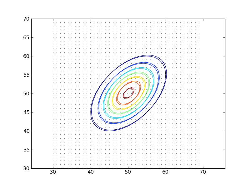
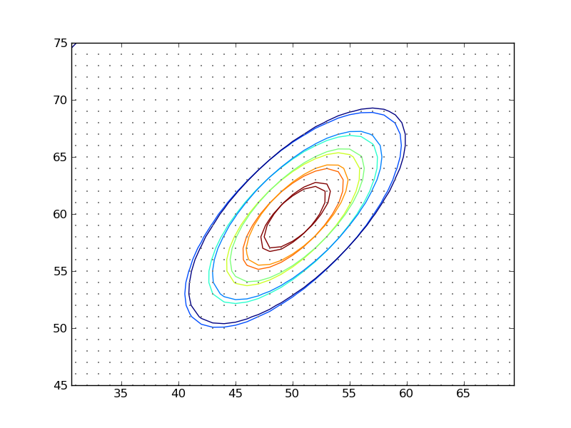
(a)	(b)
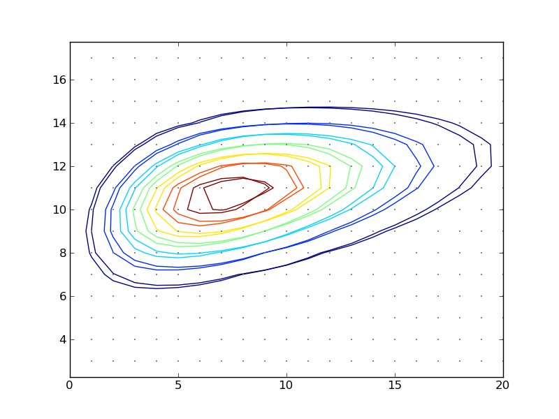
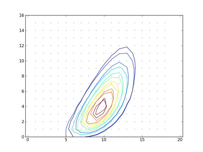
(c)	(d)

Figure 1: Contour plots for the exact and approximate pmf’s of $Gd_{2}$, for the parameters described in Table 1. The contours in all cases basically match.

	$\mu_{1}$	$v_{1}$	$\mu_{2}$	$v_{2}$	$\rho$	$\rho^{\prime}$	$K$	$\mu_{1}^{*}$	$v_{1}^{*}$	$\mu_{2}^{*}$	$v_{2}^{*}$	$\rho^{*}$
(a)	50	25	50	25	0.5	0.5144	0.99	50.25	24.99	50.25	24.99	0.5009
(b)	50	25	60	25	0.7	0.7129	0.99	50.35	25.04	59.85	24.76	0.7013
(c)	10	25	11	4	0.4	0.3988	0.99	9.45	23.30	10.90	3.85	0.3876
(d)	10	5	5	10	0.7	0.6869	0.97	10.23	4.68	5.43	10.43	0.6670

Table 1: $Gd_{2}$, resulting correlation, $\rho^{\prime}$, for the exact and resulting moments for the approximate (*) pmf of $Gd_{2}$, $gd_{2}$, with various parameters. Contour plots for the exact and approximate pmf’s of distribution (a)-(d) may be seen in Figure 1. The normalization constant needed for $gd_{2}$ is given in column $K$.

5 Discussion

We develop a generic discrete multivariate distribution defined in terms of its vector of means and variance-covariance matrix only, as it is the case for the Multivariate-Normal distribution for continuous data. This distribution has applications in the Bayesian analysis of complex models were we are dealing with counting data and the correct likelihood is not available analytically, but approximation techniques can be developed to obtain moments of observables. This is the case when studying epidemics using the SIR stochastic model, as explained in Section 1. The distribution developed here can now be used as a default distribution to be imputed to multivariate counting data in such situations. Moreover, when large counts are involved this distribution tends to a Multivariate Normal, (eg. Figure 1(a) and (b)).

References

- Alonso et al. (2007) Alonso, D., A. McKane, and M. Pascual (2007). Stochastic amplification in epidemics. Journal of the Royal Society Interface 4(14), 575.
- Andersson and Britton (2000) Andersson, H. and T. Britton (2000). Stochastic epidemic models and their statistical analysis. Springer Verlag.
- Bretó et al. (2009) Bretó, C., D. He, E. Ionides, A. King, S. Ghosal, J. Lember, A. van der Vaart, K. Triantafyllopoulos, P. Harrison, M. Ribatet, et al. (2009). Time series analysis via mechanistic models. Annals 3(1), 319–348.
- Chen and Bokka (2005) Chen, W. and S. Bokka (2005). Stochastic modeling of nonlinear epidemiology. Journal of theoretical biology 234(4), 455–470.
- Finkenstadt et al. (2002) Finkenstadt, B., O. Bjornstad, and B. Grenfell (2002). A stochastic model for extinction and recurrence of epidemics: estimation and inference for measles outbreaks. Biostatistics 3(4), 493.
- Gillespie (2007) Gillespie, D. (2007). Stochastic simulation of chemical kinetics. Annual review of physical chemistry 58(1), 35–55.
- Marin et al. (2011) Marin, J., P. Pudlo, C. P. Robert, and R. Ryder (2011). Approximate Bayesian Computational methods. Technical report, http://adsabs.harvard.edu/abs/2011arXiv1101.0955M.
- Nåsell (2002) Nåsell, I. (2002). Stochastic models of some endemic infections. Mathematical Biosciences 179(1), 1–19.
- Nelsen (2006) Nelsen, R. (2006). An introduction to copulas. New York: Springer.
- Schwartz et al. (2004) Schwartz, I., L. Billings, and E. Bollt (2004). Dynamical epidemic suppression using stochastic prediction and control. Physical Review E 70(4), 46220.
- unknonw (1978) unknonw (1978). Influenza in a boarding school. British Medical Journal 1(6112), 587.
- van Kampen (1992) van Kampen, N. (1992). Stochastic processes in physics and chemistry. North Holland.