Cosmological Parameters from Observations of Galaxy Clusters

Abstract

Studies of galaxy clusters have proved crucial in helping to establish the standard model of cosmology, with a universe dominated by dark matter and dark energy. A theoretical basis that describes clusters as massive, multi-component, quasi-equilibrium systems is growing in its capability to interpret multi-wavelength observations of expanding scope and sensitivity. We review current cosmological results, including contributions to fundamental physics, obtained from observations of galaxy clusters. These results are consistent with and complementary to those from other methods. We highlight several areas of opportunity for the next few years, and emphasize the need for accurate modeling of survey selection and sources of systematic error. Capitalizing on these opportunities will require a multi-wavelength approach and the application of rigorous statistical frameworks, utilizing the combined strengths of observers, simulators and theorists.

Keywords: cosmology, dark energy, dark matter, galaxy clusters, intracluster medium, large scale structure

1 INTRODUCTION

The statistical character of our sky’s population of clusters of galaxies, viewed from radio to gamma-ray wavelengths, is sensitive to models of cosmology, astrophysics, and large-scale gravity. Galaxy clusters are cosmographic buoys that signal locations of peaks in the large-scale matter density. The population is shallow and finite. Surveys in the coming decades will definitively map our universe’s terrain as defined by the highest $\sim\!10^{5}$ peaks. Current maps have advanced to the stage where Abell 2163, a cluster at redshift $z\sim 0.2$ with a plasma virial temperature $kT=12.27\pm 0.90\mathrm{\,keV}$ (Mantz et al. 2010a) and galaxy velocity dispersion $\sigma_{\mathrm{gal}}=1434\pm 60\mathrm{\,km}\mathrm{\,s}^{-1}$ (Maurogordato et al. 2008), has been nominated a candidate for the most massive cluster in the universe (Holz & Perlmutter 2010), the cosmic equivalent of Mount Everest.

Physically, galaxy clusters are manifested in the most massive of the bound structures – termed halos (or haloes) – that emerge in the cosmic web of large-scale structure (LSS). The LSS web is a gravitationally amplified descendant of a weak noise field seeded by quantum fluctuations during an early, inflationary epoch (Bond, Kofman & Pogosyan 1996). Its evolutionary dynamics have been well studied into the non-linear regime by N-body simulations (Bertschinger 1998). Locally bound regions (the halos) emerge, initially via coherent infall within a narrow mass range and, subsequently, via a combination of infall and hierarchical merging that widen the dynamic range, pushing to increasingly larger halo masses. The merging process is of considerable interest for cluster studies, driving astrophysical signatures that can test physical models from the nature of dark matter (Clowe et al. 2006) to the magnetohydrodynamics of hot, dilute plasmas (e.g. Kunz et al. 2011). But merging also potentially confuses cosmological studies, by creating close halo pairs that may appear as one cluster in projection and by introducing variance into observable signals.

Halos are multi-component systems consisting of dark matter and baryons in several phases: black holes; stars; cold, molecular gas; warm/hot gas; and non-thermal plasma. After decades of study via N-body and hydrodynamic simulation and related methods (see recent review by Borgani & Kravtsov 2011), models for the detailed evolution of the baryons in clusters are growing in capability to describe an increasingly large and rich volume of observations. What is clear empirically is that the galaxy formation process is globally inefficient: a recent study by Giodini et al. (2009) finds that stellar mass accounts for only $12\pm 2$ percent of the total baryon budget in the most massive halos. Radiative cooling of gas is overcome by feedback from various sources, including mechanical and radiative input from supernova winds and black hole jets, thermal conduction and other plasma processes, and ablation and harassment during gravitational encounters.

While the hierarchical nature of structure formation implies that galaxy and cluster formation are deeply intertwined and, therefore, that detailed understanding of cluster structure and evolution requires that we understand galaxy formation, the scales separating the most massive clusters from the largest galaxies – roughly a factor of 100 in length and 1000 in mass – allow progress to be made by approximate physical treatments. The dark matter kinematic structure, including remnant, fine-scale sub-halos (Moore et al. 1998; Springel et al. 2001), as well as the morphology and scaling behaviors of the hot, intracluster medium (ICM) that dominates the baryonic component (Evrard 1990; Navarro, Frenk & White 1995; Bryan & Norman 1998), are examples of areas where direct simulations made good, early progress.

A key aspect of their multi-component nature is the fact that clusters offer multiple, observable signals across the electromagnetic spectrum (e.g. Sarazin 1988). At X-ray wavelengths, the hot ICM emits thermal bremsstrahlung and line emission from ionized metals injected into the plasma by stripping and feedback processes. Stellar emission from galaxies and intracluster light dominates the optical and near-infrared. At millimeter wavelengths, inverse Compton scattering within clusters distorts the spectrum of the cosmic microwave background (CMB). Gravitational lensing offers a unique probe into the total matter distributions in clusters. Synchrotron emission from relativistic electrons is visible at radio frequencies. These and other signatures discussed below provide physically coupled, and often observationally independent, lines of evidence with which to test astrophysical models of cluster evolution. A challenge to cluster cosmology is the construction of accurate statistical models that address survey observables explicitly while incorporating intrinsic property covariance.

1.1 Clusters as Cosmological Probes

The use of clusters to study cosmology has a history dating to Zwicky’s discovery of dark matter in the Coma Cluster (Zwicky 1933). Brightest cluster galaxies were later employed as standard candles to study the local expansion history of the universe; Hoessel, Gunn & Thuan (1980) actually derived (with low significance) a negative deceleration parameter using this approach, implying accelerated expansion consistent with present findings. In the 1980’s, measurement of the enhanced spatial clustering of clusters relative to galaxies supported the model of Gaussian random initial conditions expected from inflation (Bahcall & Soneira 1983). In the early 1990’s, an apparent discrepancy between local baryon fraction measurements of clusters (Fabian 1991; Briel, Henry & Boehringer 1992) with primordial nucleosynthesis expectations helped rule out a model with critical matter density (White et al. 1993). The revelation of hot clusters at high redshift later that decade (Donahue et al. 1998; Bahcall & Fan 1998) presaged the ultimate discovery of dark energy from Type Ia supernova (SNIa) surveys. The turn of the millennium witnessed a flurry of activity aimed at measuring the amplitude of the matter power spectrum from cluster counts. X-ray studies in particular showed that the amplitude was lower than had been accepted previously (e.g. Borgani et al. 2001; Reiprich & Böhringer 2002; Seljak 2002; Pierpaoli et al. 2003; Allen et al. 2003; Schuecker et al. 2003), a result later confirmed by CMB and cosmic shear measurements. These studies also exposed the importance of understanding systematic effects associated with the use of directly observable quantities as proxies for mass (Henry et al. 2009).

Recent studies have used cluster counts or the ICM mass fraction in very massive systems (both methods described in more detail below) to constrain cosmological parameters. These studies are consistent with other observations that find a universe dominated by dark energy ($73\%$), with sub-dominant dark matter ($23\%$), and a small minority of baryonic material ($4.6\%$) (Komatsu et al. 2011). A detailed pedagogical treatment of how cluster studies helped establish this reference cosmology is given in the review of Voit (2005). Rosati, Borgani & Norman (2002) review X-ray studies of clusters from the ROSAT satellite era.

Explaining the nature of the dark energy and dark matter are core problems of physics. The consensus ‘concordance’ cosmological model, $\Lambda$CDM, postulates that dark energy (DE) is associated with a small, non-zero vacuum energy, equivalent to a cosmological constant term in Einstein’s equations. Another possibility is that DE arises from a light scalar field (or fields) that evolves over cosmic time. A third option is that DE is essentially an apparition, not a source term of Einstein’s general relativistic equations but a reflection of their breakdown at length and time scales of cosmic dimensions (e.g. Copeland, Sami & Tsujikawa 2006). Sky surveys of cosmic systems, from supernovae to galaxies to clusters of galaxies, provide the means to discriminate among these alternatives.

Forthcoming cluster surveys at mm, optical/near-infrared, and X-ray wavelengths, discussed in Section 6.1, have the potential to find hundreds of thousands of groups and clusters. Figure 1 puts these efforts into historical perspective, by plotting size against year of publication for cluster samples that generated cosmological constraints discussed in this review. Symbol size is proportional to median sample redshift, and symbol types encode the selection method. The stars at far right show theoretical estimates of the all-sky number and median redshift of halos with masses above $10^{14}\,M_{\odot}$ and $10^{15}\,M_{\odot}$. The former mass limit roughly marks the transition from galaxy groups to galaxy clusters, while the latter marks the deepest potential wells with ICM temperatures $kT\ {\raise-3.22916pt\hbox{$\buildrel>\over{\sim}$}}\ 5\mathrm{\,keV}$. Current surveys have made good progress, but the full population of clusters remains largely undiscovered.

Optical and X-ray surveys have the longest histories, but these traditional methods are being complemented by new approaches. Space-based surveys in the near-infrared extend optical methods to $z>1$ (Eisenhardt et al. 2008; Demarco et al. 2010), and the first few clusters identified by their gravitational lensing signature have been published (Wittman et al. 2006). Ongoing mm surveys have released the first sets of clusters discovered through the Sunyaev-Zel’dovich (SZ) effect (Marriage et al. 2010; Vanderlinde et al. 2010; Planck Collaboration 2011a), with the promise of much more to come.

Panoramic, multi-wavelength surveys of common sky areas offer profound improvements to our understanding of clusters as astrophysical systems, which in turn further empowers their use for cosmological studies. And while considerable challenges to interpretation and modeling of survey data certainly exist, a halo model framework, discussed in Section 2, is rising to meet this task.

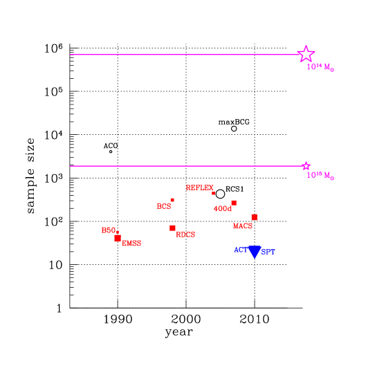
Figure 1: Yields from modern surveys of clusters used for cosmological studies are shown, with symbol size proportional to median redshift. Samples selected at optical (circles), X-ray (red squares), and mm (blue triangles) wavelengths are discussed in Section 3.2 . Stars and horizontal lines show full sky counts of halos expected in the reference $\Lambda$CDM cosmology (see Section 2) with masses above $10^{15}$ and $10^{14}\,M_{\odot}$. Such halo samples have median redshifts of $0.4$ and $0.8$, respectively.

1.2 Cosmic Calibration via Simulations

A feature common to many techniques that study DE is the nature of the input data, which consists of catalogs of properties, $\mathbf{x}$, of discrete objects that lie along our past light-cone. Upcoming wide-field surveys will generate $\mathbf{x}$-catalogs of large dimension that will be distilled to constrain perhaps tens of cosmological and astrophysical parameters. Such catalogs may contain internal support through the use of complementary methods: besides galaxy clusters (CL), the same data set can be analyzed for baryon acoustic oscillations (BAO) and, for optical surveys, weak lensing (WL). (In the case of repeat observations, optical surveys can also be analyzed for Type Ia supernovae and gravitational time delay signatures.) Science processing leads to a compressed set of statistical signals, $\mathbf{y}_{i}$, where $i$ indicates an aforementioned method. For large cluster surveys, $\mathbf{y}$ might consist of counts of clusters binned by sky area, redshift and detected signal.

Extracting accurate constraints on a set of cosmological model parameters, $\bm{\theta}$, from these surveys requires sophisticated likelihood analyses. The critical ingredient is $p(\mathbf{y}_{i}|\bm{\theta})$, the underlying likelihood that the CL (and other) statistics of the observed sky would be realized within a particular universe. Key capabilities that enable such likelihood analysis are:

1. to predict statistical expectations, $p(\mathbf{y}_{i}|\bm{\theta})$, for many universes, $\bm{\theta}$;
   

2. to extract unbiased statistical signals from the raw catalog, $\mathbf{y}_{i}(\mathbf{x})$;
   

3. to understand the expected signal covariance, COV($\mathbf{y}_{i},\mathbf{y}_{j}).$

Genuine understanding of cosmological models from observed cluster data is dependent on the degree to which theory and simulation can provide robust predictions for the observed signals. While numerical simulations of LSS can predict catalog-level yields for a given cosmology (e.g. Springel, Frenk & White 2006), such predictions necessarily entail additional astrophysical assumptions, meaning $p(\mathbf{y}_{i}|\bm{\theta})$ is actually $p(\mathbf{y}_{i}|\bm{\theta},\bm{\alpha})$, where $\bm{\alpha}$ represents degrees of freedom introduced by an assumed astrophysical model. Recovering cosmological information from survey data therefore necessitates marginalization over a reasonable range of astrophysical assumptions. On the other hand, as cosmological constraints from all methods improve, the cluster community can potentially invert the problem, recovering constraints on astrophysical models after marginalizing over cosmology.

We begin this review by describing the theoretical basis for cluster cosmology (Section 2), and include there an opening discussion of important sources of systematic error. Key observational windows are described in Section 3, and recent cosmological constraints are reviewed in Section 4. In Section 5, cluster contributions to particle physics and gravity are examined. In Section 6, we highlight opportunities for important, near-term progress. In closing, we emphasize some essential considerations in survey modeling and analysis (Section 7) before presenting our conclusions (Section 8).

2 THEORETICAL BASIS

This section sketches a theoretical description of the halo framework that supports cluster cosmology. There is considerable richness to the galaxy formation problem that we omit here; the recent review of Benson (2010) provides substantial detail. Simulation studies of halo evolution into the strongly non-linear regime are becoming increasingly powerful, but finite resolution and uncertainty in astrophysical treatments limit predictive power. While not yet robust enough to offer sharp prior characterization of the astrophysics required for cosmological studies, simulations offer key insights into the structure and physics sensitivity of the functions that relate observable signals to halo mass and epoch.

2.1 LSS and Halo Formation from Inflation

Ample evidence now supports the picture that LSS formed via gravitational amplification of initially small density fluctuations, $\delta\equiv(\rho-\bar{\rho})/\bar{\rho}$. Cosmic microwave background anisotropy measurements are consistent with expectations from a large class of basic inflationary models (e.g. Baumann & Peiris 2009). Such models are characterized by an instantaneous primordial power spectrum, $P_{\rm prim}(k)\sim|\delta_{k}(a)^{2}|\sim k^{n_{\mathrm{s}}}$, with spectral index, $n_{\mathrm{s}}$, expected to be close to unity. Here, $\delta_{k}$ is the Fourier transform of the density fluctuations, $\delta(\mathbf{x})$.

After inflation ceases, fluctuations in the coupled photon-baryon-dark matter fluid evolve in ways that are now well understood from linearized Boltzmann treatments (Seljak et al. 2003). For the standard case of adiabatic fluctuations, and on scales above the baryon Jeans mass, the post-recombination matter (dark matter and baryons) power spectrum exhibits a growing mode that scales with the cosmic expansion parameter, $a$, as

$$P_{\mathrm{m}}(k,a,\bm{\theta_{\Omega}})=G^{2}(a,\bm{\theta_{\Omega}})\,T^{2}(k,\bm{\theta_{\Omega}})\,P_{\rm prim}(k).$$ (1)

Here, $T(k,\bm{\theta_{\Omega}})$ is a transfer function that encapsulates evolution before recombination at $z\sim 1100$, $G(a,\bm{\theta_{\Omega}})$ is the density perturbation growth factor from linear theory, and $\bm{\theta_{\Omega}}$ is the controlling parameter set of the background cosmological model. Dark energy models that involve modifications to general relativity may introduce $k$-dependence into the growth function above.

The power spectrum in the reference $\Lambda$CDM model is set by present-epoch energy densities, $\bm{\theta_{\Omega}}=\{\Omega_{\mathrm{b}}h^{2},\Omega_{\mathrm{c}}h^{2},\Omega_{\Lambda}\}$, where $h=H_{0}/100\mathrm{\,km}\mathrm{\,s}^{-1}\mathrm{\,Mpc}^{-1}$ is the dimensionless Hubble constant and $\Omega_{X}\equiv\rho_{X}/\rho_{\mathrm{cr}}$ is the density of component $X$ relative to the critical density, $\rho_{\mathrm{cr}}=3H_{0}^{2}/8\pi G$. The curvature density, $1-\sum_{X}\Omega_{X}$, is zero to within $\pm 0.007$ (Komatsu et al. 2011), consistent with a flat spatial metric on cosmic scales. Our notation uses ‘b’ for baryons, ‘c’ for cold, dark matter (CDM), and ‘m’ for all matter: $\Omega_{\mathrm{m}}=\Omega_{\mathrm{b}}+\Omega_{\mathrm{c}}$. In the minimal model, the dark energy is a vacuum energy with equation of state, $p=-\rho c^{2}$. We use $\Omega_{\Lambda}$ for this case and employ $\Omega_{\mathrm{DE}}$ when referring to models wherein the dark energy equation of state, $w=p/(\rho c^{2})$, differs from $-1$.

Table 1: Flat $\Lambda$CDM Parameters^a from WMAP+BAO+$H_{0}$

Parameter	Value
$\Omega_{\Lambda}$	$0.725\pm 0.016$
$\Omega_{\mathrm{c}}$	$0.229\pm 0.015$
$\Omega_{\mathrm{b}}$	$0.0458\pm 0.0016$
$h$	$0.702\pm 0.014$
$n_{\mathrm{s}}$	$0.968\pm 0.012$
$10^{10}\Delta_{\cal R}^{2}(k_{0})$	$0.2430\pm 0.0091$
$\sigma_{8}$	$0.816\pm 0.024$
a From Komatsu et al. (2011).

Current constraints for a flat $\Lambda$CDM model from CMB measurements, combined with angular clustering of red galaxies and local measurements of $H_{0}$, are shown in Table 1 (Komatsu et al. 2011). The parameter $\Delta_{\cal R}^{2}(k)$ is the variance in density fluctuations evaluated at horizon crossing, which is independent of $k$ for $n_{\mathrm{s}}=1$, and the wavenumber $k_{0}=0.002\mathrm{\,Mpc}^{-1}$ corresponds to a large comoving length scale, $\sim\pi/k_{0}=1.6\mathrm{\,Gpc}$.

In the minimal model, the matter density fluctuations filtered within a sphere of comoving radius $R$ are Gaussian distributed with zero mean. The comoving radius defines a mass, $M=(4\pi/3)\rho_{\mathrm{cr}}R^{3}$, of matter within that radius in the young universe, when $\Omega_{\mathrm{m}}(a)=1$. Early observations that the variance in galaxy counts is near unity on a scale of $R=8\hbox{$\,h^{-1}$}\mathrm{\,Mpc}$ led to this as a conventional choice of scale at which to quote the fluctuation amplitude (see Table 1 ). The corresponding mass, $M=0.59\times 10^{15}\hbox{$\,h^{-1}$}\,M_{\odot}$, is characteristic of rich clusters of galaxies.

The variance of linearly-evolved, CDM fluctuations, filtered on mass scale $M$, has the form

$$\sigma^{2}(M,a)=\int\,\frac{d^{3}k}{(2\pi)^{3}}\ W^{2}(kR)\ P_{\mathrm{m}}(k,a).$$ (2)

where the filter function is $W(y)=3[\sin(y)/y^{3}-\cos(y)/y^{2}]$ for the typical case of sharp (or top-hat) spatial filtering within radius $R$. Evaluating Equation 2 at $8\hbox{$\,h^{-1}$}\mathrm{\,Mpc}$ and $a=1$ produces the oft-quoted matter power spectrum normalization parameter, $\sigma_{8}$. We will see below that $\sigma(M,a)$ serves as a similarity variable for expressing model-independent forms of the halo space density and clustering.

The evolution of the fluctuation spectrum, Equation 1, is valid at early times or at scales sufficiently large so that $\sigma(M,a)\ll 1$ at all times. On small scales, where CDM power spectra are generically maximum, fluctuation growth produces $\delta\geq 1$, and linear theory breaks down. Mode-mode coupling terms become important to the dynamics, and solutions in Fourier space become difficult. While higher-order perturbation theory solutions can extend analytic evolution to later times than linear theory (e.g. Bernardeau et al. 2002; Crocce & Scoccimarro 2006), the full problem is typically treated using N-body simulations, discussed below.

A recent analytical advance considers LSS as an effective fluid. Baumann et al. (2010) show that integrating out small-scale, non-linear structures renormalizes the cosmological background and introduces dissipative terms, of order $v^{2}/c^{2}$, into the dynamics of large-scale modes, with $v$ the typical velocity dispersion of collapsed halos. Since even the most massive halos have $v<0.01c$, the magnitude of these effects is very small. Furthermore, Baumann et al. (2010) show that virialized halos decouple completely from large-scale dynamics, at all orders in the post-Newtonian expansion.

2.1.1 HALO MODEL DESCRIPTION OF LSS

Astrophysical structures, from the first stars at high redshift to galaxy clusters at low redshift, tend to emerge from local maxima of the filtered density field. While density peaks are generally non-spherical (Bardeen et al. 1986), a first-order description considers them spherical and isolated from their surroundings. Birkhoff’s theorem then implies that the expansion histories of radial mass shells within a peak follow trajectories perturbed from the overall background, with sufficiently dense shells expanding to a maximum size and then contracting. The traditional ansatz assumes collapse by a radial factor of two (Gunn & Gott 1972), after which a quasi-virialized and quasi-hydrostatic structure – a perfectly spherical halo – is born.

The collapse criterion is that the linearly-evolved perturbation amplitude reach a critical value, $\delta(a)=\delta_{\mathrm{c}}$, with $\delta_{\mathrm{c}}=1.686$ the conventional choice. Applying this idea to the CDM spectrum, Equation 2, leads to a characteristic mass scale, $M_{\ast}(a)$, defined by $\sigma[M_{\ast}(a),a]=\delta_{\mathrm{c}}$. At a given epoch, a spectrum of halo masses exist, with masses above (below) $M_{\ast}(a)$ forming from perturbations with amplitudes above (below) the rms level of the filtered Gaussian spectrum. Considerable literature (e.g. Press & Schechter 1974; Bond et al. 1991; Bond & Myers 1996; Sheth & Tormen 1999, and many others) has established this picture as the halo model of large-scale structure. We review here only aspects relevant for cluster cosmology; a more thorough review can be found in Cooray & Sheth (2002).

The basic element of the halo model is the population mean space density, $n(M,z)$, in units of number per unit comoving volume, commonly referred to as the mass function. Expressed as a differential function of mass, it takes the form

$$\frac{dn}{d\,{\rm ln}\,M}=\frac{\bar{\rho}_{\mathrm{m}}}{M}\,\left|\frac{d\,{\rm ln}\,\sigma}{d\,{\rm ln}\,M}\right|\,f(\sigma),$$ (3)

where $\bar{\rho}_{\mathrm{m}}=\Omega_{\mathrm{m}}\rho_{\mathrm{cr}}$ is the comoving mean matter density and $f(\sigma)$ is a model-dependent function of the filtered perturbation spectrum, Equation 2. Analytic forms for $f(\sigma)$ capture much, but not all, of the behavior seen in N-body simulations, as discussed below.

The spatial clustering of halos is described by a modified version of the matter power spectrum. On large spatial scales, or low wavenumbers, the halo autocorrelation power spectrum is modified,

$$P_{\rm hh}(k,a)=b^{2}(M,a)\,P_{\mathrm{m}}(k,a),$$ (4)

where $b(M,a)$, the halo bias function, is independent of $k$, for the case of Gaussian fluctuations, but dependent on mass and epoch. While this expression applies to the spatial autocorrelation of systems with fixed mass $M$, it generalizes to the cross-correlation between sets of halos at different masses, $P_{\rm h1h2}(k,a)=b(M_{1},a)b(M_{2},a)\,P_{\mathrm{m}}(k,a)$. The theory of peaks in Gaussian random fields expresses the bias as a function of the normalized peak height, $\nu=\delta_{\mathrm{c}}/\sigma(M,a)$ (Kaiser 1984; Bardeen et al. 1986).

Below, we show that N-body simulations support the forms of equations (3) and (4), but a precise fit to the mass function requires that $f(\sigma)$ be adjusted to include explicit redshift dependence, $f(\sigma,z)$. There are subtleties to the definition of mass in simulations that must also be taken into account.

2.1.2 ASTROPHYSICAL PROCESSES

Various astrophysical processes play out within the photon-baryon components of the evolving cosmic web, including hydrodynamic, magnetohydrodynamic and radiative transfer effects; star and black hole formation with associated feedback of momentum, energy and entropy; and so on. Except for the immediate vicinity of black holes, these processes involve classical physics that is largely known. But the fully three-dimensional and non-linear nature of the problem, the wide dynamic range in length and time scales, and the non-trivial couplings among the constituent physical processes introduce tremendous complexity into baryon evolution. Galaxy formation is truly a Grand Challenge computational problem. We touch on select issues relevant to the observable features of galaxy clusters.

Shocks and turbulent MHD heating. During halo formation, gravitational potential energy in the baryonic component is thermalized via shocks. The highest Mach numbers, of tens or more, should occur in the accretion shocks at the edges of clusters (e.g. Pfrommer et al. 2006). While these strong shocks are expected to be efficient particle accelerators, recent observations place tight limits on the volume-averaged pressure contributions from relativistic particles (Ackermann et al. 2010). Shocks with Mach numbers of a few are also associated with major mergers: a spectacular example is the narrow radio relic in the cluster CIZA J2242.8+5301, for which van Weeren et al. (2010) use multi-frequency radio and polarization observations to infer a Mach number $4.6^{+1.3}_{-0.9}$ in a shock located $1.5\mathrm{\,Mpc}$ from the cluster center. Most of the energy thermalized during cluster formation, however, is dissipated in weak shocks that are persistently driven by dissipating sub-structures and ongoing minor mergers. Shocks are also driven by jets from AGNs and, at earlier times, by winds from star forming galaxies.

Details of the nano-parsec scale physics that drive thermalization remain under active study, especially the roles of magnetic fields, turbulence and plasma instabilities (e.g. Kunz et al. 2011). Observations and simulations discussed below indicate that thermalization is efficient; thermal pressure supplies the bulk of support against gravity within the halo potential except during brief periods near periapsis of major mergers.

Radiative cooling. Since the intracluster plasma (and, to a lesser extent, its interstellar counterpart) is optically thin at most wavelengths, radiation loss is the primary cooling mechanism for the baryonic component of halos. Indeed, the classic criterion for setting an upper bound on galaxy size comes from balancing the gas cooling time against the halo dynamical time (White & Rees 1978). The first generation of stars form at $z\sim 30$, aided by molecular hydrogen line emission, within halos of mass $\sim\!10^{6}\,M_{\odot}$ (Abel, Bryan & Norman 2002; Bromm et al. 2009). By $z\sim 10$, atomic line cooling in halos with virial temperatures above $10^{4}$ K produces the first generation of galaxies, which grow hierarchically for a time determined by the large-scale environment. Proto-cluster regions have more efficient cooling at high redshift than do proto-voids, but the feedback from vigorous, early production of compact sources helps to quench star formation before a large fraction of baryons are converted to stars.

The cooling timescale of the gas in massive halos is typically longer than a Hubble time, except for a subset of systems that exhibit cool cores. The central $\sim 100\mathrm{\,kpc}$ region of such systems tends to be X-ray bright and typically contains a dominant elliptical galaxy. We discuss aspects of cool core phenomenology in Section 6.4.

Star and black hole formation. Cold, molecular gas fuels star formation. The star formation rate can roughly be considered as proportional to the local rate of gas cooling below $10^{4}$ K, but there are other considerations. Different venues for star formation exist, ranging from quiescent disks to the bulges of tidally-triggered starburst galaxies, and it is not yet clear whether a single model based on local gas conditions captures the full range of observed behavior. Supermassive black hole (SMBH) growth occurs through mergers and accretion in galactic cores, and these central engines drive quasar and radio jet activity (e.g. Di Matteo, Springel & Hernquist 2005). Sloan Digital Sky Survey (SDSS) quasar studies indicate that SMBHs of mass $\sim 10^{9}\,M_{\odot}$ exist at $z=7$ (Fan 2006), and processes for forming such large black holes in the first few hundred million years of the universe have been proposed (Volonteri 2010).

In Gaussian random fields, small-scale peaks are more abundant when embedded within large-scale peaks, so the largest galaxies and quasars at high redshift represent the progenitors of massive galaxies observed in low redshift clusters.

Feedback from compact sources. Feedback of mass, momentum, and entropy from stellar/SMBH sources is important at all stages of the LSS hierarchy. Photoionization and supernova-driven winds serve to limit cooling and star formation in low-mass halos (Dekel & Silk 1986). Jets driven by accretion onto the central SMBH appear to be required to limit the maximum size of galaxies (e.g. Croton et al. 2006; Cattaneo et al. 2009). Formulations for this feedback typically tie the energy input to the mass accretion rate which, in turn, is governed by the local rate of cooling and/or cold accretion.

The end result of this competition between cooling and heating is that heating largely wins. The overall efficiency of star formation is small, and peaks in halos of roughly galactic scale (e.g. Moster et al. 2010). Figure 2 shows a recent compilation of stellar mass fraction ($M_{\rm star}/M$) measurements as a function of halo circular velocity, $v_{\rm circ}=\sqrt{GM/r}$, with $M$ the total halo mass and $r$ its radius (Dai et al. 2010). The horizontal lines show the cosmic baryon fraction, $\Omega_{\mathrm{b}}/\Omega_{\mathrm{m}}=0.171\pm 0.009$, derived from Wilkinson Microwave Anisotropy Probe (WMAP) data analysis (Dunkley et al. 2009).

Figure 2: The observed stellar mass fraction as a function of halo circular velocity for systems ranging from galaxies to rich clusters indicates that star formation efficiency peaks in halos of mass $\sim\!10^{13}\hbox{$\,h^{-1}$}\,M_{\odot}$. From Dai et al. (2010).

The stellar mass fraction is maximized at a few tens of percent of the cosmic mean in halos with $v_{\rm circ}\sim 300\mathrm{\,km}\mathrm{\,s}^{-1}$, equivalent to a mass of $10^{13}\hbox{$\,h^{-1}$}\,M_{\odot}$ at $z=0$. In cluster-sized halos, the stellar fraction declines with mass, taking on values $\sim 10\%$ of the global baryon fraction at the highest masses. Yet, the largest galaxies are found in the cores of massive clusters, and their very old stellar populations produce a characteristically narrow ‘red sequence’ in a color-magnitude diagram of cluster members.

Dynamical and thermodynamical equilibrium. In the context of the evolving cosmic web, the processes above must contend with conditions imposed by halo merging. At any given time, major mergers, such as those involving progenitor pair mass ratios larger than $0.3$, occur in $\sim 10\%$ of the population, concentrated toward the highest masses. These rare events can drive the mass contents of a halo considerably out of equilibrium.

Minor mergers, while much more frequent, are also less damaging. Current simulations and observations indicate that the dynamical and thermodynamical response of halos is quite fast. Hydrostatic and virial equilibrium assumptions are typically valid to within roughly ten percent for the majority of the cluster population (e.g. Rasia et al. 2006; Nagai, Vikhlinin & Kravtsov 2007).

All this astrophysical evolution offers a treasure trove of observational possibilities. Uniquely in massive clusters, all of the matter is readily observed, allowing a complete census to be taken. Stars make up 1–3% (Lin & Mohr 2004; Gonzalez, Zaritsky & Zabludoff 2007; Giodini et al. 2009); $\sim\!15\%$ resides in the hot, diffuse, intergalactic gas (Allen et al. 2008; Simionescu et al. 2011); and the rest is in the form of non-baryonic CDM (Section 5.1).

2.2 Cosmological Tests with Massive Halos

As tracers of massive halos, galaxy clusters provide a number of signatures that are sensitive to the underlying cosmology. We review here the principles underlying key methods. A typical set of cosmological parameters for such studies might consist of the primordial spectrum amplitude and slope, the present-epoch densities of the three energy components dominant at late times, the dimensionless Hubble constant, and the DE equation of state parameters,

$$\bm{\theta}\ =\ \left\{n_{\mathrm{s}},\Delta_{\cal R}^{2},\Omega_{\mathrm{b}}h^{2},\Omega_{\mathrm{c}}h^{2},\Omega_{\mathrm{DE}},h,w_{0},w_{a}\right\},$$ (5)

where the last two parameters define a linearly-evolving DE equation of state,

$$w(a)=w_{0}+w_{a}(1-a).$$ (6)

This particular set is meant to be illustrative. There is considerable variation in the literature, and many works restrict analysis to a flat cosmology, which removes one degree of freedom from the above through the condition $\Omega_{\mathrm{b}}+\Omega_{\mathrm{c}}+\Omega_{\mathrm{DE}}=1$.

2.2.1 HALO COUNTS AND CLUSTERING

The yield of upcoming cluster surveys will be sufficiently large to enable disaggregation by angular position, redshift, and the observed signal, $S$. (Note the latter is also referred to in the literature as the mass proxy, or sometimes the observable mass, $M_{\mathrm{obs}}$.) Complications associated with the signal–mass likelihood and with redshift estimation are discussed below. As a starting point, consider a perfect tracer of mass, $S=M$, with error-free redshifts, $z_{\mathrm{est}}=z$. Within a given survey, the expected number of halos, $\bar{N}_{ai}$, in a cell described by mass bin $a$ and redshift bin $i$ with solid angle $\Delta\Omega$ is

$$\bar{N}(M_{a},z_{i})\equiv\bar{N}_{ai}=\frac{\Delta\Omega}{4\pi}\int_{z_{i}}^{z_{i+1}}dz\,\frac{dV}{dz}\ \int_{\ln M_{a}}^{\ln M_{a+1}}\,d\,{\rm ln}\,M\ \frac{dn}{d\,{\rm ln}\,M}.$$ (7)

Cosmology enters this expression through the mass function and the volume element, $dV/dz$.

The counts in each large spatial bin will deviate from the mean by an excess number, $b(M_{a},z_{i})\delta(\mathbf{x})$, determined by the local large-scale density field, $\delta(\mathbf{x})$. Following Cunha, Huterer & Doré (2010), the spatial covariance of the counts is

$$C^{a}_{ij}=\left\langle\left(N_{ai}-\bar{N}_{ai}\right)\left(N_{aj}-\bar{N}_{aj}\right)\right\rangle=\bar{N}_{ai}\bar{N}_{aj}\xi^{a}_{ij},$$ (8)

where $\xi^{a}_{ij}$ describes the spatial correlation between mass-redshift bins,

$$\xi^{a}_{ij}=\int\,\frac{d^{3}k}{(2\pi)^{3}}\left|W_{i}(\mathbf{k})W_{j}(\mathbf{k})\right|f\left({\mathbf{k}\cdot\bm{\Delta}\mathbf{x}}\right)\,b_{ai}b_{aj}\,P_{\mathrm{m}}(k,z).$$ (9)

Here, $W_{i}$ is the window function for cell $i$ (that, when present, can include the effects of redshift estimate uncertainties) and $f$ is a geometric term that depends on the comoving separation, $\bm{\Delta}\mathbf{x}$, between cells $i$ and $j$. When cells $i$ and $j$ sample different redshifts, an accurate approximation uses their geometric mean to evaluate $P_{\mathrm{m}}(k,z)$ (Cunha, Huterer & Doré 2010).

Combining the spatial clustering with a diagonal shot noise term forms the full covariance for a survey sample. Derivatives of the mean counts and covariance with respect to model parameters form the Fisher information matrix used in survey forecasts. Expressions for the Fisher matrix can be found in Hu & Cohn (2006).

Equations (7) through (9) serve as the foundation of likelihood analysis of large cluster surveys. To be useful in practice, these expressions must undergo a number of modifications, including: transformation from mass to the signal used for cluster detection, $p(S|M,z)$; inclusion of counting errors arising from incompleteness (missed sources) and impurities (false sources); and inclusion of photometric uncertainties, $p(z_{\mathrm{est}}|z)$. We discuss these issues in Section 2.5 and summarize current results in Section 4.1.

2.2.2 BARYON FRACTION AS A STANDARD QUANTITY

The mass fraction of hot gas, $f_{\mathrm{gas}}$, measured within a characteristic radius of a halo at redshift $z$ can be written as

$$f_{\mathrm{gas}}(z)=\Upsilon(z)\left(\frac{\Omega_{\mathrm{b}}}{\Omega_{\mathrm{m}}}\right),$$ (10)

where $\Upsilon(z)$ accounts for star formation and other baryon effects within that radius. At large radii in the most massive halos, where the hot ICM dominates the baryon budget and the impacts of feedback processes are modest, baryon losses are small and $|1-\Upsilon|\ {\raise-3.22916pt\hbox{$\buildrel<\over{\sim}$}}\ 0.1$ is a reasonable expectation.

Motivated by the growing body of measurements of $f_{\mathrm{gas}}$ from the ROSAT X-ray satellite, Sasaki (1996) and Pen (1997) recognized that a mismatch in the dependence on metric distance, $d$, between gas mass ($\propto d^{5/2}$) and total mass ($\propto d$) measured from X-ray observations implied that gas fraction measurements in massive clusters could be exploited as a distance estimator, with $f_{\mathrm{gas}}(z)\propto d(z)^{3/2}$. Like Type Ia supernovae, massive clusters serve as standard calibration sources that test the expansion history of the universe. Key benefits, relative to survey counts, are the ability to perform this test with a relatively small number of clusters and the relative insensitivity to cluster selection. We summarize results from this exercise in Section 4.2.

2.2.3 DISTANCES FROM JOINT X-RAY AND SZ OBSERVATIONS

In a similar vein, Silk & White (1978) noted that X-ray and SZ measurements could be combined to determine distances to clusters. The CMB spectral shift is governed by the Compton y-parameter, a measure of the electron pressure along the line of sight, $y\propto\int dx\,n_{\rm e}(x)T(x)$. Given an observed SZ signal, $y_{\rm obs}$, and a predicted signal based on X-ray measurements of the ICM density and temperature, $y_{\rm pred}$, the angular diameter distance scales as

$$d_{\mathrm{A}}\propto\left(\frac{y_{\rm obs}}{y_{\rm pred}}\right)^{2}.$$ (11)

The cosmological constraint originates from the distance dependence of the X-ray measurements, $y_{\rm pred}(z)\propto d(z)^{1/2}$, and the requirement that $y_{\rm pred}=y_{\rm obs}$. Accurate SZ and X-ray flux and temperature calibration are particularly important to this method, referred to below as XSZ.

2.2.4 ANGULAR THERMAL SZ POWER SPECTRUM

The thermal and kinetic SZ signals from clusters (Section 3.1.3) cause distortions in the CMB at small angular scales ($\ell\!\sim\!1000$). If the distortion pattern from a single halo of mass $M$ at redshift $z$ is described by an angular Fourier transform, $\tilde{y}(M,z,\ell)$, then the full halo population will generate a fluctuation spectrum (Shaw et al. 2010)

$$C_{\ell}\propto\int\,dz\,\frac{dV}{dz}\ \int\,d\,{\rm ln}\,M\ \frac{dn}{d\,{\rm ln}\,M}\ \tilde{y}^{2}(M,z,\ell).$$ (12)

Adding halo spatial correlations gives a small correction to this estimate (Komatsu & Seljak 2002). This approach to testing cosmology is limited by degeneracy with astrophysical assumptions, as the interplay between $\tilde{y}(M,z,\ell)$ and $dn/d\,{\rm ln}\,M$ makes clear.

2.2.5 BULK FLOWS

Measurements of the cosmic peculiar velocity field contain additional cosmological information (e.g. Strauss & Willick 1995 and references therein). The kinetic SZ effect (Section 3.1.3) in principle offers a way to measure the peculiar velocities of galaxy clusters. Although some initial results based on such measurements have been reported (e.g. Kashlinsky et al. 2008, 2010; Keisler 2009; Osborne et al. 2010), the technique has not yet reached the maturity of those discussed above and is not discussed further in this review.

2.3 Halo Model Calibration via Simulations

N-body simulations of a single, collisionless dark matter fluid offer the means to investigate non-linear evolution of LSS under an implicit ‘light-traces-mass’ assumption. The technology supporting such simulations has advanced to the state where $N=10^{12}$ is available (but not yet realized) on peta-scale computational platforms (Pope et al. 2010). Employing larger-$N$ simply to model bigger volumes is a natural mode of growth, since parallelization is relatively simple (large-volume domain decomposition minimizes the particle transfer among computational nodes), the number of timesteps is independent of $N$, and the light-traces-mass assumption is easier to justify under modest mass and force resolution. Large-volume simulations produce generous halo population realizations with which to calibrate the mass function and clustering of halos, and current state-of-the-art studies employ ensembles of $10^{9-10}$-particle simulations.

Coupled N-body and gas dynamic simulation methods enable multi-fluid studies that break free of the light-traces-mass assumption. Indeed, the first application of this class of codes tested the possible separation of baryons and neutrinos within clusters formed in a universe dominated by massive neutrinos (Evrard & Davis 1988). The field has advanced considerably since then, and we refer the reader to Borgani & Kravtsov (2011) for a recent review. We discuss primarily dark matter simulations here, with some relevant multi-fluid simulations results presented in the next section.

2.3.1 MEASURES OF HALO MASS

Through the mass function, halo mass provides the critical measure that connects observables to the underlying cosmology. But halos are complex, dynamic structures that confound attempts at a unique definition of mass.

In the model of spherical collapse applied to initial density peaks, the halo edge and interior mass are readily defined by the outermost caustic in dark matter or by the location of the shock in cold baryonic accretion (Bertschinger 1985). In both cases, this radius marks an abrupt transition in the mean radial velocity, separating a nearly hydrostatic interior from an infall-dominated exterior. Halos forming in 3-D simulations deviate from this ideal case in important ways, some of which can be described by higher-order analytic approaches to peak evolution (Bond & Myers 1996). The collapse process is more ellipsoidal than spherical, and merging competes with smooth accretion as the dominant mode of halo growth (e.g., Fakhouri & Ma 2010). Defining centers and boundaries in this complex environment has become a matter of convention.

Two common algorithmic conventions have emerged: (i) percolation, also known as friends-of-friends (FOF), and (ii) spherical overdensity (SO). FOF first links all pairs of particles within a given distance, $b$, then merges them into groups based on a shared link condition (‘a friend of a friend is a friend’). The SO approach first filters the particle field to identify peaks, then grows spheres around peaks with sizes determined by an interior density threshold, $3M(<r_{\Delta})/(4\pi r_{\Delta}^{3})=\Delta\rho_{\rm t}$. The threshold density $\rho_{\rm t}$ is typically chosen to be either the background matter density, $\rho_{\rm t}=\bar{\rho}_{\mathrm{m}}(z)$, or the critical density, $\rho_{\rm t}=\rho_{\mathrm{cr}}(z)$. Unless otherwise specified, we adopt the latter convention in this article.

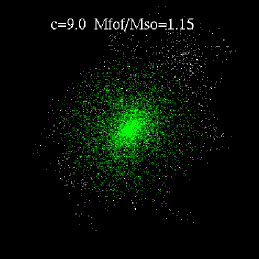
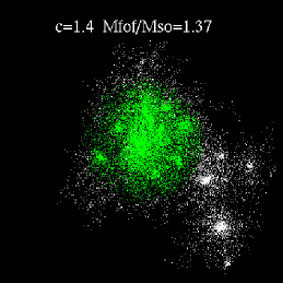
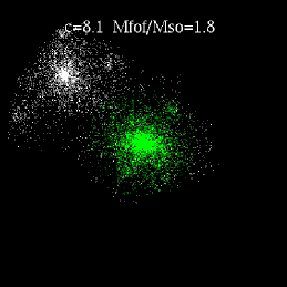
Figure 3: Three examples of halos identified under both FOF (white and green colored particles) and SO (green only) algorithms. The mass ratio for each case is given, as is the concentration parameter, $c$, derived from a radial density fit. See text for details. Adapted from Lukić et al. (2009).

Several studies discuss the relative merits of these approaches and argue values for the parameters $b$ and $\Delta$ (e.g. Cole & Lacey 1996; White 2001; Lukić et al. 2009). Figure 3 provides a visualization of three simulated halos spanning a range of dynamical and morphological behaviors. In each panel, white particles are members of the FOF halo with $b=0.2(V/N)^{1/3}$ while green are SO members using $\Delta=200$ against $\rho_{\mathrm{cr}}(z)$. These are typical of parameter values used in the literature. The left panel shows a relatively isolated system where the two methods give fairly consistent results. The other panels show two discrepant cases; in the middle is a highly-structured, active merger while, at right, percolation across a filamentary bridge links two similarly sized systems that are just beginning to merge.

The discrepant cases do not dominate in number, but neither are they uncommon. For cosmological studies, what is important is to establish an accurate accounting process to enumerate observable halo features. Roughly speaking, observers viewing the systems in Figure 3 would be likely to identify one dominant cluster in the left and middle panels, and two in the right. An FOF accounting system would need to admit a non-unitary condition (one halo maps to two clusters) when converting mass to observable signals. In contrast, SO masses map to integrated aperture observations more directly. For this reason, SO masses see more frequent use for survey data analysis.

2.3.2 HALO MASS FUNCTION AND CLUSTERING

The original multiplicity function paper of Press & Schechter (1974) used the clustering of particles in N-body experiments with $N=1000$ to support their analytic form for $f(\sigma)$ in Equation 3. Later, Sheth & Tormen (1999) used $N=10^{7}$ simulations to set free parameters of their $f(\sigma)$ model derived using an ellipsoidal, rather than spherical, collapse approximation. Using a suite of simulations of open and flat cosmologies with $\Omega_{\mathrm{m}}$ ranging from $0.3$ to 1, Jenkins et al. (2001) found a unique, three-parameter form for $f(\sigma)$ that produced a mass function accurate to $\sim\!30\%$ across the suite of models.

A recent study by Tinker et al. (2008) employs 22 large ($N\sim 10^{9}$) simulations produced with three independent N-body codes to calibrate a functional form motivated by Sheth & Tormen (1999),

$$f(\sigma)=A\left[\left(\frac{\sigma}{b}\right)^{-a}+1\right]\,e^{-c/\sigma^{2}}.$$ (13)

This study was the first to open the density threshold degree of freedom; their fitting parameters are published as functions of $\Delta$ (against $\bar{\rho}_{\mathrm{m}}(z)$) for $\Delta\in[200,3200]$. With the high statistical power of their simulation ensemble, Tinker et al. (2008) achieve a fit with $5\%$ statistical precision in halo number at $z=0$ for a $\Lambda$CDM cosmology. Maintaining this precision for redshifts $z\leq 2.5$ requires the introduction of mild redshift dependence into the fit parameters, $A(z)$, $a(z)$ and $b(z)$. The theoretically expected halo counts above masses $M_{200}=10^{14}$ and $10^{15}\,M_{\odot}$ in the reference $\Lambda$CDM cosmology, shown in Figure 1, are based on the Tinker form for threshold $\Delta=200$ against the mean mass density (see fitting formulae in Mortonson, Hu & Huterer 2011).

On the other hand, the bias function measured in the same simulation ensemble shows no need for such redshift-dependent corrections. Framed in terms of the normalized linear perturbation amplitude, $\nu\!\propto\!\sigma(M)^{-1}$, Tinker et al. (2010) find a robust fit of the form

$$b(\nu)=1-D\frac{\nu^{d}}{\nu^{d}+\delta_{\mathrm{c}}^{d}}+E\nu^{e}+F\nu^{f},$$ (14)

with a single set of parameters $\{d,e,f,D,E,F\}$ that are written only as functions of $\Delta$. For the case $\nu=3$ (i.e., $3\sigma$ peaks), the value of the bias is large, $b\sim 6$, for $\Delta=200$. The cluster power spectrum, Equation 4, can be enhanced by factors of several tens over the mass power spectrum.

The very massive end of the FOF mass function was recently revised by Crocce et al. (2010) using $2048^{3}$-particle simulations in $\Lambda$CDM cubic volumes up to $7680\hbox{$\,h^{-1}$}\mathrm{\,Mpc}$ in scale. Above $10^{15}\hbox{$\,h^{-1}$}\,M_{\odot}$, their fit lies up to $30\%$ above prior calibrations (Jenkins et al. 2001; Warren et al. 2006).

2.3.3 INTERNAL HALO STRUCTURE

Gravitational relaxation drives the phase-space structure of halos to a common structure that applies from small galactic satellites to the most massive galaxy clusters. The form of the radial density,

$$\rho(r)={{\rho_{\mathrm{cr}}(z)\,A_{c}}\over{({r/r_{\rm s}})\,\left(1+{r/r_{\rm s}}\right)^{2}}},$$ (15)

is known as the Navarro-Frenk-White (NFW) profile (Navarro, Frenk & White 1995). Here, $r_{\rm s}$ is the scale radius, $c$ is the concentration parameter (with $c=r_{200}/r_{\rm s}$) and $A_{c}={200c^{3}/3\left[{{\rm ln}(1+c)-{c/(1+c)}}\right]}$.

Simulations show that concentration and mass are weakly correlated. In the mass range of galaxies to clusters, $c\propto M^{-\zeta}$, with $\zeta\sim 0.14$ at $z=0$ and $\zeta\rightarrow 0$ at $z\ {\raise-3.22916pt\hbox{$\buildrel>\over{\sim}$}}\ 3$ (e.g., Gao et al. 2008). That study finds that a fixed concentration, $c\sim 4\pm 1$, applies in the mean to high mass halos, independent of redshift. Tracking the mass accretion histories of halos in simulations, Wechsler et al. (2002) find a common functional form, and show that the formation epoch correlates strongly with concentration. The concentration–mass relation can be understood as a result of adiabatic contraction of differently-shaped peaks in the linear density field (Dalal, Lithwick & Kuhlen 2010).

2.4 From Halos to Clusters: Mass Proxies, Scaling Relations and Projection Effects

Cluster cosmology originates from phenomena observed on the sky, in the 2+1 space of angular coordinates and redshift. The observables employed for a likelihood analysis must be predicted under a set of combined cosmological and astrophysical parameters, $\{\bm{\theta},\bm{\alpha}\}$. For constraints based on cluster counts, the mass function, $n(M,z)$, written in terms of spherical overdensity or percolation measures from simulations needs to be translated into a signal function, $n(\mathbf{S},z)$, for one or more signals, $S_{i}$. We use the terms signal and observable interchangeably, and generically they refer to bulk measures at mm (SZ decrement $Y$), optical (richness, $N_{\rm gal}$, or velocity dispersion, $\sigma_{\rm gal}$), or X-ray (luminosity, $L_{\mathrm{X}}$; temperature, $T_{\mathrm{X}}$; gas mass, $M_{\mathrm{gas}}$; and/or gas thermal energy, $Y_{\mathrm{X}}=kT_{\mathrm{X}}M_{\mathrm{gas}}$) wavelengths (see Section 3). An ideal experiment would measure all of these observables within apertures optimally matched to the underlying halo sizes, $r_{\Delta}(M,z)$. This ideal is often frustrated by signal-to-noise constraints and confused by projection effects and foreground/background contamination.

2.4.1 OBSERVABLE SIGNAL LIKELIHOOD FROM MULTIVARIATE SCALING RELATIONS

Scaling relations for cluster signals, based on assumptions of virial equilibrium and self-similar internal structure, were first published by Kaiser (1986). In this model, halos at fixed mass and redshift are identical, and scalings with mass and redshift follow calculated power-law behaviors. Observations generally support power-law behavior, but not always with the self-similar slope (Section 4.1.3). We describe here a non-self-similar model that incorporates arbitrary mass scaling and allows for variations at fixed mass and redshift.

For compactness of notation, let $s_{i}=\ln(S_{i})$, for each of the $N$ observables, $S_{i}$, and let $\mu=\ln M$. The power-law assumption transforms to log-linear scaling

$$\mathbf{\bar{s}}(\mu,z)\ =\ \mathbf{m}\mu\ +\ \mathbf{b}(z),$$ (16)

where the average is over a very large cosmic volume. The elements of $\mathbf{m}$ are the slopes of the individual mass-observable relations, and the intercepts $\mathbf{b}(z)$ reflect the evolution at fixed mass. At a fixed epoch, we can always choose units such that $b_{i}(z)=0$ (as we do below). For cosmological studies, a measure of merit is the equivalent mass scatter in each signal, $\sigma_{\mu i}\equiv\sigma_{i}/m_{i}$.

Various processes, including different formation histories and the stochastic nature of mergers, generate deviations from the mean. Taking these as Gaussian in the log leads to a form for the conditional signal likelihood,

$$p\left(\mathbf{s}|\mu,z\right)\ =\ \frac{1}{(2\pi)^{N/2}|\Psi|^{1/2}}\exp\left\{-\frac{1}{2}\left[\mathbf{s}-\mathbf{\bar{s}}(\mu,z)\right]^{\dagger}\mathbf{\Psi}^{-1}\left[\mathbf{s}-\mathbf{\bar{s}}(\mu,z)\right]\right\}.$$ (17)

The elements of the covariance matrix, $\Psi_{ij}\equiv\left\langle(s_{i}-\bar{s}_{i})(s_{j}-\bar{s}_{j})\right\rangle$, could have mass or redshift dependence, but a first-order approach considers them as constants.

When the mass variance of signals is small, $\sigma_{\mu i}^{2}\ll 1$, then the above expressions can be convolved with a locally power-law approximation to the mass function, $n(\mu,z)=Ae^{-a\mu}$, to obtain the local signal space density function,

$$n(\mathbf{s},z)\ =\ \frac{A\Sigma}{(2\pi)^{(N-1)/2}|\Psi|^{1/2}}\exp\left[-\frac{1}{2}\left(\mathbf{s}^{\dagger}\Psi^{-1}\mathbf{s}-\frac{\bar{\mu}^{2}}{\Sigma^{2}}\right)\right],$$ (18)

where $\Sigma^{2}=\ (\mathbf{m}^{\dagger}\Psi^{-1}\mathbf{m})^{-1}$ is the variance about the mean log-mass selected by the set of signals $\mathbf{s}$,

$$\bar{\mu}(\mathbf{s},z)\ =\ \frac{\mathbf{m}^{\dagger}\Psi^{-1}\mathbf{s}}{\mathbf{m}^{\dagger}\Psi^{-1}\mathbf{m}}-a\Sigma^{2}\ \equiv\ \bar{\mu}_{0}(\mathbf{s},z)-a\Sigma^{2}.$$ (19)

The first term above is the mean mass for the case of a flat mass function, $a=0$. The second term, represents the (Eddington) mass bias induced by asymmetry in the mass function convolution. Upscattering of low-mass systems dominates when $a>0$, and the high-mass end of the $\Lambda$CDM  mass function is steep, $a\ {\raise-3.22916pt\hbox{$\buildrel>\over{\sim}$}}\ 3$ (Mortonson, Hu & Huterer 2011). These equations make explicit the degeneracy between cosmology (e.g. $A$ and $a$) and astrophysics (e.g. $\mathbf{m}$ and $\Psi$) inherent in cluster counts. They provide the means to compute biases, relative to a mass complete sample, associated with signal-limited cluster samples (discussed further in Section 2.5.1).

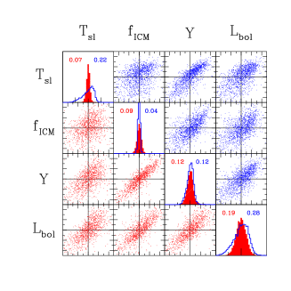
Figure 4: Left: Covariance of internal properties of $>\!4500$ halos with $M_{200}>5\times 10^{13}\hbox{$\,h^{-1}$}\,M_{\odot}$ extracted from Millennium Gas Simulations produced under two different physical treatments. Off-diagonal panels show normalized ($(s_{i}-\bar{s}_{i})/\sigma_{i}$) pairwise deviations under preheating (PH, lower) and gravity-only (GO, upper) treatments; large tickmarks are separated by unity. Diagonal panels show the distribution of ln(property) deviations for PH (red) and GO (blue) models, with dispersions given in the legend. Right: Visual representation of the mass variance, Equation 20, obtained using the property pairs at left. The radii scale with $\Sigma$, and a $5\%$ reference is shown in the upper left. Adapted from Stanek et al. (2010).

Figure 4 provides support for this model from Millennium Gas Simulation analysis (Stanek et al. 2010). The left panel shows deviations about the mean behavior of four intrinsic (3-dimensional) properties measured within $r_{200}$ for $>\!4500$ halos with mass $M_{200}>5\times 10^{13}\hbox{$\,h^{-1}$}\,M_{\odot}$ at $z=0$. The lower diagonal and red histograms show results from a cooling and preheating (PH) treatment of the baryons, where the entropy is instantaneously raised to $200\mathrm{\,keV}\,{\rm cm}^{2}$ at $z=4$. Only a small fraction of baryons cool into stars in this model (Young et al. 2011). The upper diagonal and blue histograms are from a gravity-only (GO) treatment, where the gas is heated only by shocks and does not cool.

The internal properties generally have modest variance, and pairs tend to be positively correlated with typical correlation coefficient $r\sim 0.4-0.8$. Halos identified by a pair of properties will have mass variance

$$\Sigma^{2}\ =\ (1-r^{2})\left(\sigma_{\mu 1}^{-2}+\sigma_{\mu 2}^{-2}-2r\sigma_{\mu 1}^{-1}\sigma_{\mu 2}^{-1}\right)^{-1},$$ (20)

shown by the areas of the off-diagonal circles in the right panel of Figure 4. Individual properties lie along the diagonal. The intrinsic gas thermal energy, $Y$, selects mass with $7\%$ dispersion, the best individual measure for both physics cases. This level is also seen in the simulations of Nagai (2006) which include cooling, star formation and feedback. Pairs of intrinsic measurements always improve mass selection, and the strong correlation between $f_{\mathrm{ICM}}$ and $Y$ combines with the large mass variance of $f_{\mathrm{ICM}}$ to achieve mass selection with $4\%$ scatter in the PH model.

Applying Bayes’ theorem to this model allows one to write the likelihood of mass and an observable, $s_{2}$, for a sample selected on observable $s_{1}$. When the two signals are correlated, one can show that the scaling with mass of the non-selection signal will be

$$\bar{s}_{2}(s_{1})\ =\ m_{2}\left[\bar{\mu}(s_{1})+\alpha r\sigma_{\mu 1}\sigma_{\mu 2}\right],$$ (21)

which is biased relative to the naive expectation of $m_{2}s_{1}/m_{1}$. The intrinsic correlation between signals at fixed mass is relatively challenging to constrain from current data, but first measurements have been made for samples selected using optical (Rozo et al. 2009) and X-ray (Mantz et al. 2010a) observations.

2.5 From Theory to Practice: Sources of Systematic Error

Clusters on the sky relate to halos through selection on one or more observables. Matching cluster detections (which originally reside in a 2+1 space of angular position and signal-to-noise) to halos can sometimes be complex; two halos along nearly the same line of sight may be blended into a single cluster, or a single halo may be fragmented into more than one cluster. The frequency of these occurrences is typically not large, $\ {\raise-3.22916pt\hbox{$\buildrel<\over{\sim}$}}\ \!10\%$, but the exact values are sensitive to a number of factors, particularly detection method and mass, and so are best modeled via direct sky realizations (e.g. Sehgal et al. 2011).

The selection observable can be distorted from its intrinsic value (Equation 17) by triaxiality, by additional sources along the line-of-sight, by mis-centering and/or mis-estimation of the radial scale, and by other effects. Telescope/instrument calibration and data processing methods also contribute to the error budget. For upcoming studies using cluster counts, photometric redshift errors have an important, but not dominant, effect (Section 6.1).

2.5.1 SAMPLE SELECTION

Testing cosmology with halo counts and clustering requires that the theoretical mass function be transformed, via the scaling relations and a model of the selection process, into a prediction for the distribution of clusters in the space of survey observables (e.g. redshift and X-ray flux). The scaling relation parameters set the space density portion of the survey yield (Equation 18) in terms of the (cosmologically dependent) local amplitude, $A(\mu,z)$, and logarithmic slope, $a(\mu,z)$, of the mass function. Sample selection must be well understood to avoid perturbing $A(\mu,z)$ and $a(\mu,z)$ from their true values, biasing cosmological results. Fortunately, such effects can be mitigated by survey self-calibration (Majumdar & Mohr 2004) or by calibration using follow-up observations, as discussed below.

The task of empirically constraining the scaling relations is complicated by the fact that the clusters targeted for follow-up observations are themselves subject to selection effects related to their original discovery. In an X-ray flux-limited sample, for example, higher X-ray luminosity at a given mass leads to a larger probability of detection (commonly known as Malmquist bias). The effects of selection bias must therefore be accounted for in the calibration of scaling relations, much as in the cosmological analysis (e.g. Stanek et al. 2006; Sahlén et al. 2009).

      

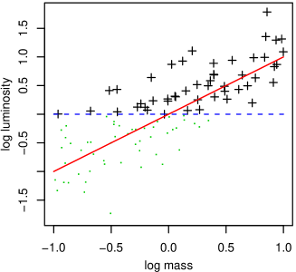
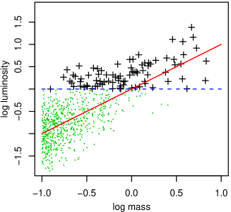
Figure 5: Cartoon illustrating generically how the distribution of observed scaling relation data (black crosses) do not reflect the underlying scaling law (red line) due to selection effects (e.g. a luminosity threshold; blue, dashed line). Green dots indicate undetected sources. The left panel shows an unphysical case in which cluster log-masses are uniformly distributed, while the mass function in the right panel is a more realistic, steeper power-law (normalized to produce roughly the same number at high masses). The steepness of the mass function has a clear effect on the degree of bias in the detected sample. To recover the correct scaling relation, an analysis must account for both the selection function of the data and the underlying mass function of the cluster population. Adapted from Mantz et al. 2010a.

Figure 5 illustrates the influence of selection on observed scaling relation data in a cartoon case. The full population (black crosses and green points) obeys a scaling law (red line) with non-trivial intrinsic scatter. In the simple case where detection requires a particular threshold luminosity (the dashed, blue line), it can be seen that, even if every detected cluster is followed up to obtain precise measurements of the mass and luminosity, the resulting data set will be a biased representation of the full population. While complete at the highest masses, the sample is increasingly incomplete at low masses, with the low-luminosity systems absent.

A closely related consideration is the effect of the underlying mass function on the observed scaling relation data. The distribution of the relation’s independent variable(s) (in this case cluster masses) within the full population generically influences constraints on scaling laws (e.g. Gelman et al. 2004; Kelly 2007). Neglecting to account for this influence corresponds to the assumption of uniformly distributed independent variables; often this approximation is sufficient, but the exponentially steep slope of the cluster mass function suggests that we should take the issue seriously in the context of cluster cosmology (Mantz et al. 2010b). Figure 5 illustrates how the steepness of the mass function influences the fraction of the observed data which are strongly biased relative to the underlying scaling relation. Given the need to solve for both the slope and scatter of the scaling relation, accounting for the disparity in the number of high-mass and low-mass systems is critical. We note that simply conditioning the sampling distribution on cluster detection, as some authors have done, is not sufficient to rigorously recover all the scaling information.

Note that this effect has a floor set by non-zero intrinsic scatter in the scaling relations, but the effect can in principle be enhanced by measurement error. However, measurement errors in current X-ray and optical cluster surveys are typically smaller than the intrinsic dispersion, even at the survey limit. Thus, re-measurement of the survey observables through deeper, follow-up observations (e.g. to improve the signal-to-noise of X-ray or SZ flux) does not circumvent the issue of selection bias in the scaling relation analysis.

While selection bias clearly influences scaling relations involving the selection observable, it also influences relations of other signals with which the selection observable has non-zero intrinsic correlation (Equation 21). This is illustrated in Figure 6, for a signal which is correlated with the selection observable with coefficient 0.1 (left panel) and 0.9 (right panel). The red line shows the true scaling law and the points shown correspond to the detected clusters from Figure 5 (right panel). With relatively mild intrinsic correlation, as has been found for temperatures and soft X-ray flux detection (Mantz et al. 2010a), the distribution of data points closely follows the underlying relation; for more extreme values of the correlation coefficient, as might be expected, e.g., between temperature and SZ signal, deviations due to selection bias become evident. Note that the severity of the effect also depends on the covariance of the signals rather than only on the correlation coefficient (i.e. the size of the marginal scatter in each signal is also important).

      

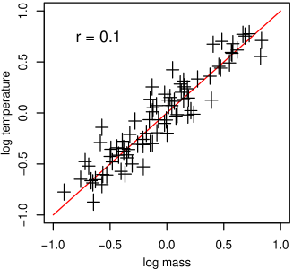
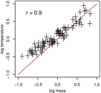
Figure 6: Cartoon scaling relations where the observable of interest is not the basis of cluster selection. In both panels, the red line indicates the true scaling relation, and the black crosses correspond to the detected clusters in the right panel of Figure 5. The marginal scatter in this relation is chosen to be smaller than that in Figure 5, consistent with measured values of the luminosity–mass and temperature–mass intrinsic scatters (Section 3.3.4). The intrinsic temperature–luminosity correlation at fixed mass is relatively small in the left panel ($r=0.1$) and large in the right panel ($r=0.9$); in the latter case, the observed data are significantly influenced by selection bias despite the fact that the selection was made using a different observable.

Cluster samples are often characterized in terms of completeness and purity (White & Kochanek 2002). Completeness is used in many ways, but its simplest form for cluster cosmology refers to the fraction of halos above mass $M$ at redshift $z$ that are identified in a survey with some observable limit, $S_{\rm lim}(z)$. Completeness of unity is achievable at high masses when the survey limit, $S_{\rm lim}(z)$, lies sufficiently far in the signal likelihood’s negative tail. Impurity is a measure of false positive sources in the sample. Fewer conventions for its definition exist in the literature. Generically, one can write the observed counts above some signal limit $S$ as a sum, $N_{\rm obs}(>S)=N_{\rm true}(>S)+N_{\rm false}(>S)$, where the first term represents genuine cluster systems – manifestations of a single massive halo along the line of sight – and the second expresses detections of other origin. Zero impurity, $N_{\rm false}(>S)=0$, is a desired goal.

2.5.2 PROJECTION EFFECTS

Telescopes aimed at a distant halo necessarily collect photons that originate elsewhere along the multi-gigaparsec sightline than within the target system. Due to their softer angular profiles, SZ, lensing and optical cluster signals can be blended more readily than X-ray. Chance orientations of two or more halos within local supercluster regions create an asymmetric tail to high signal values. Considered in terms of mass selection, the effect produces a tail to low masses in the distribution of halo mass selected at a given signal (e.g. Cohn et al. 2007).

Since the matter components of halos are generally ellipsoidal rather than spherical, orientation variations also produce scatter in signals observed in halos of fixed mass. Signals are generally maximized when viewed along the long axis and minimized along the short axis. Orientation can affect cluster selection, with prolate systems oriented along the line-of-sight being preferentially included. Since its collisional nature drives the X-ray emitting gas toward equipotential surfaces, it tends to be rounder than the dark matter and so less susceptible to orientation bias.

As discussed in Section 3, the density squared dependence of the X-ray emissivity means that X-ray selection is less prone to projected confusion. Optical richness measurements roughly trace mass density and are therefore more easily confused by projection and orientation effects. SZ measurements are intermediate, since the SZ effect depends on electron pressure, the product of density and temperature.

2.6 Non-Standard Scenarios

It is important to keep in mind that theory offers many potential deviations from the reference $\Lambda$CDM cosmology sketched above. Key model assumptions – that the dark matter is a weakly interacting massive particle, that inflation produced a Gaussian spectrum of initial density fluctuations with a power-law initial spectrum, that small-amplitude metric perturbations are well described by Newtonian, weak field expansions in general relativity, and so on – need to be rigorously tested. In Section 5, we discuss ways in which clusters can be used to test a number of proposed modifications to the reference model.

3 OBSERVATIONAL TECHNIQUES

In this section we review briefly the physics underlying multiwavelength observations of galaxy clusters. We summarize efforts to construct cluster catalogs, with an emphasis on surveys that have led to cosmological constraints. We discuss techniques used to measure the masses of clusters, and observable proxies that correlate tightly with mass.

3.1 Multiwavelength Measurements of Galaxy Clusters

3.1.1 X-RAY OBSERVATIONS

Most of the baryons in the Universe are in diffuse gas. Typically, this gas is very difficult to observe. Within galaxy clusters, however, gravity squeezes the gas, heating it to virial temperatures of $10^{7}$–$10^{8}\mathrm{\,K}$, which causes it to shine brightly in X-rays. Galaxy clusters therefore ‘light up’ at X-ray wavelengths as luminous, continuous, spatially-extended sources (Figure 7).

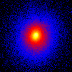
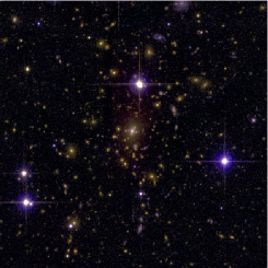
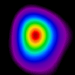
Figure 7: Images of Abell 1835 ($z=0.25$) at X-ray, optical and mm wavelengths, exemplifying the regular multi-wavelength morphology of a massive, dynamically relaxed cluster. All three images are centered on the X-ray peak position and have the same spatial scale, 5.2 arcmin or $\sim 1.2\mathrm{\,Mpc}$ on a side (extending out to $\sim r_{2500}$; Mantz et al. 2010a). Figure credits: Left: X-ray: Chandra X-ray Observatory/A. Mantz; Center, Optical: Canada France Hawaii Telescope/A. von der Linden et al.; Right, SZ: Sunyaev Zel’dovich Array/D. Marrone.

The primary X-ray emission mechanisms from the diffuse ICM are collisional: free-free emission (bremsstrahlung); free-bound (recombination) emission; and bound-bound emission (mostly line radiation). The emissivities of these processes are proportional to the square of the electron density, which ranges from $\sim 10^{-1}\mathrm{\,cm}^{-3}$ in the centers of bright ‘cool core’ clusters to $\sim 10^{-5}\mathrm{\,cm}^{-3}$ in cluster outskirts. At these low densities, the X-ray emitting plasma is optically thin and in the coronal limit, which makes modeling straightforward.

For survey observations, the primary X-ray observables are flux, spectral hardness and spatial extent. Using deeper, follow-up observations of individual clusters, modern X-ray satellites allow the spatially-resolved spectra of clusters to be determined precisely, permitting measurements of the density, temperature and metallicity profiles of the ICM, and a host of derived thermodynamic quantities. For reviews of the principles underlying X-ray observations of clusters see, e.g., Sarazin (1988) and Böhringer & Werner (2010).

3.1.2 OPTICAL AND NEAR INFRARED OBSERVATIONS

The optical and near-IR emission from galaxy clusters is predominantly starlight. The galaxy populations of clusters are dominated by ellipticals and lenticulars (i.e. early-type galaxies). This is particularly true in the central regions, where the largest and most luminous galaxies are found (Figure 7).

The old and relatively homogeneous nature of their stellar populations leads to the majority of the galaxies in clusters occupying relatively tight loci in color-magnitude diagrams (e.g. Bower, Lucey & Ellis 1992). This characteristic has proved important to modern cluster finding algorithms.

For optical surveys of clusters, the main observables are the richness (i.e. the number of galaxies within the detection aperture), luminosity and color. For follow-up observations of individual clusters, aimed in particular at measuring their masses, the primary observables are the galaxy number density, luminosity, and velocity dispersion profiles. Typical velocity dispersions for large clusters are of order 1000$\mathrm{\,km}\mathrm{\,s}^{-1}$.

For reviews of optical studies of galaxy clusters including discussions of the development of the field, see Bahcall (1977) and Biviano (2000).

3.1.3 SZ OBSERVATIONS

As CMB photons pass through a galaxy cluster they have a non-negligible chance to inverse Compton scatter off the hot ICM electrons. This scattering boosts the photon energy and gives rise to a small but significant frequency-dependent shift in the CMB spectrum observed through the cluster known as the thermal Sunyaev-Zel’dovich (hereafter SZ or tSZ) effect (Sunyaev & Zeldovich 1972). The magnitude of the effect is proportional to the line of sight integral of the product of the gas density and temperature. The kinetic SZ (kSZ) effect is an additional, smaller distortion of the CMB spectrum due to the peculiar motion of a cluster with respect to the Hubble Flow (i.e. the CMB rest frame). The magnitude of the kSZ effect is proportional to the peculiar velocity. For a review see Carlstrom, Holder & Reese (2002).

3.1.4 GRAVITATIONAL LENSING

According to general relativity, the gravity associated with a mass concentration will bend light rays passing near to it in a phenomenon known as gravitational lensing. This can both magnify and distort the images of background galaxies. With modern data, gravitational lensing can be detected clearly in the statistical appearance of background galaxies observed through clusters (weak lensing), and in the field (often termed cosmic shear). Occasionally, lensing can also lead to strong distortions and multiple images of individual sources (strong lensing). For a galaxy cluster and background galaxies of known redshifts, the measured gravitational shear can be used to infer the cluster mass. For a recent review of gravitational lensing, see Bartelmann (2010).

3.2 Constructing Cluster Catalogs

A well-designed cluster survey should meet requirements in terms of angular scale, flux sensitivity and redshift coverage. The survey should be as complete (i.e. not have missed clusters that it should have detected) and pure (i.e. not have detected spurious clusters) as possible and the selection function describing the completeness and purity as a function of signal, position and redshift should be known precisely. The survey observables should correlate as tightly as possible with mass. In tension with these requirements, surveys must also be constructed within the context of limited resources.

3.2.1 X-RAY SURVEYS

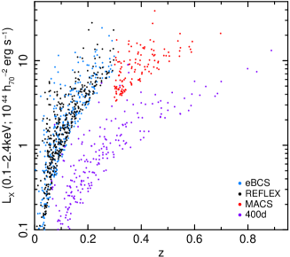
Figure 8: X-ray luminosities and redshifts for four ROSAT cluster catalogs – extended BCS (blue; Ebeling et al. 1998, 2000), REFLEX (black; Böhringer et al. 2004), MACS (red; Ebeling, Edge & Henry 2001; Ebeling et al. 2007, 2010), and 400d (purple; Burenin et al. 2007) – sub-samples of which have been used in cosmological studies.

X-ray observations currently offer the most mature and powerful technique for constructing cluster catalogs. The primary advantages of X-ray surveys are their exquisite purity and completeness, and the tight correlations between X-ray observables and mass.

Galaxy clusters are simple to identify at X-ray wavelengths, being the only X-ray luminous, continuous, spatially extended, extragalactic X-ray sources. Clusters have typical soft X-ray band luminosities of $10^{44}$ erg/s or more, and spatial extents of several arcmin or larger, even at high redshifts. Given modest angular resolution, e.g. $\Delta\theta\sim 1$ arcmin (full width half maximum, FWHM; easily achievable) and tens of detected counts, the X-ray emission from galaxy clusters can be detected against a background populated otherwise only sparsely with point-like active galactic nuclei.

The first X-ray cluster catalogs constructed for cosmological work (Edge et al. 1990, often called the ‘Brightest 50’ or B50 catalog; Gioia et al. 1990) were based on the Ariel V and HEAO-1 all-sky surveys, and pointed observations made with the Einstein Observatory and EXOSAT (see also Lahav et al. 1989). These catalogs provided early evidence for evolution in the X-ray luminosity function of clusters (Edge et al. 1990; Gioia et al. 1990; Henry et al. 1992) and were used subsequently in a series of pioneering cosmological works (e.g. Henry & Arnaud 1991; Viana & Liddle 1996; Kitayama & Suto 1996; Henry 1997; Eke et al. 1998).

These catalogs were eventually superseded by surveys carried out with the ROSAT satellite. This mission, launched in June 1990, had two main parts: the ROSAT All-Sky Survey (RASS; Voges et al. 1999), spanning the first 6 months; and pointed observations, which took place over the next 8 years. The main instrument aboard ROSAT, the Position Sensitive Proportional Counter, had a modest point spread function (PSF; $\sim 1$ arcmin FWHM in survey mode), but low background and a wide field of view ($\sim 2$ degree diameter).

The main cluster catalogs constructed from the RASS and used in cosmological studies include the ROSAT Brightest Cluster Sample (BCS; Ebeling et al. 1998), which covered the northern hemisphere at high Galactic latitudes and low redshifts ($z<0.3$) to a flux limit of $4.4\times 10^{-12}$ $\mathrm{\,erg}\mathrm{\,cm}^{-2}\mathrm{\,s}^{-1}$(0.1–2.4 keV); the ROSAT-ESO Flux-Limited X-ray Galaxy Cluster Survey (REFLEX; Böhringer et al. 2004), which covered the southern sky at low redshifts to a flux limit of $3.0\times 10^{-12}$ $\mathrm{\,erg}\mathrm{\,cm}^{-2}\mathrm{\,s}^{-1}$  in the same band; the HIFLUGCS sample (Reiprich & Böhringer 2002) of the X-ray brightest clusters at high Galactic latitudes, with $F_{\rm X}>2.0\times 10^{-11}$ $\mathrm{\,erg}\mathrm{\,cm}^{-2}\mathrm{\,s}^{-1}$(0.1–2.4keV); and the Massive Cluster Survey (MACS; Ebeling et al. 2010), which extended this work to higher redshifts $0.3<z<0.5$ and slightly fainter fluxes $F_{\rm X}>2.0\times 10^{-12}$ $\mathrm{\,erg}\mathrm{\,cm}^{-2}\mathrm{\,s}^{-1}$. Other cluster surveys have been constructed from the RASS, or are in the process of being constructed, but have not yet been used to derive rigorous cosmological constraints.

A number of X-ray cluster catalogs have also been constructed based on serendipitous discoveries in the pointed phase of the ROSAT mission. Notable among these are the ROSAT Deep Cluster Survey (RDCS; Rosati et al. 1998) and the 400 Square Degree ROSAT PSPC Galaxy Cluster Survey (400d; Burenin et al. 2007), which have been used to derive cosmological constraints. These catalogs cover much smaller areas than the RASS, but reach an order of magnitude or more fainter in flux (Figure 8).

A second major advantage of X-ray surveys is the observed strong correlation between X-ray luminosity and mass across the entire flux and redshift range of interest. These quantities follow a simple power law relation (Section 4.1.3), with a dispersion in luminosity at a given mass of $\sim 40\%$ and no significant outliers (Mantz et al. 2010a). The density-squared dependence also makes the X-ray survey signal from clusters relatively insensitive to projection effects. Thus, an X-ray survey of sufficient depth can be translated straightforwardly into statistical knowledge of the distribution of massive halos.

In principle, X-ray surveys could be constructed using even lower-scatter mass proxies (Section 3.3.4) such as temperature or center-excised luminosity as the survey observable. However, given the ease and depth to which total X-ray luminosity can be measured, these lower-scatter mass proxies are typically used as auxiliary data (e.g. Mantz et al. 2010b; Wu, Rozo & Wechsler 2010).

The primary disadvantage of X-ray cluster surveys is that they can only be carried out from space, which makes their construction relatively expensive.

3.2.2 OPTICAL SURVEYS

The first extensive cluster catalog was constructed at optical wavelengths by George Abell (Abell 1958) based on visual inspection of photographic plates from the Palomar Observatory Sky Survey. Abell identified clusters as concentrations of 50 or more galaxies in a magnitude range m3 to m3+2 (where m3 is the magnitude of the third brightest cluster member) and radius $R_{\mathrm{A}}=1.5h^{-1}$ Mpc (with distance estimated based on the magnitude of the tenth brightest galaxy). Clusters were further characterized into richness and distance classes. Abell’s catalog was updated and extended to the southern sky by Abell, Corwin & Olowin (1989) (hereafter ACO). The final ACO sample has more than 4000 clusters. An additional, early optical cluster catalog extending to poorer systems was compiled by Zwicky and collaborators (see e.g. Zwicky, Herzog & Wild 1961), although the search criteria were less strict than Abell’s.

Huchra & Geller (1982) applied a percolation algorithm to an early CfA redshift catalog to identify a set of 92 nearby groups and clusters. Using 4-m class telescopes and a mix of photographic plate and CCD observations, (Gunn, Hoessel & Oke 1986) opened high redshift cluster studies by identifying 418 systems over $\sim\!150$ deg² extending out to $z=0.92$. Spatial and photometric matched filter methods (e.g. Postman et al. 1996) as well as the introduction of N-body simulations to calibrate projection effects (e.g. van Haarlem, Frenk & White 1997) marked the beginning of the modern era of optical cluster cosmology.

Because the cores of galaxy clusters are dominated by red, early-type galaxies, an effective way to reduce the impact of projection effects is to use color information to select for overdensities of red galaxies (e.g. Gladders & Yee 2005, and references therein). The Red-Sequence Cluster Survey (RCS), a sample of 956 clusters identified with a single ($R_{c}-z^{\prime}$) color, provided the first modern cosmological constraints using optical selection (Gladders et al. 2007).

To cover a broad range of redshifts, multi-color photometry is needed to track the intrinsic 4000 angstrom break feature of old stellar populations as it reddens. The five-band photometry of the Sloan Digital Sky Survey (SDSS) enabled such selection. The maxBCG catalog (Koester et al. 2007) of 13,823 clusters with optical richness $\hbox{$N_{\rm gal}$}\geq 10$ was produced using $g-r$ colors and spans the redshift range $0.1<z<0.3$. Cosmological constraints from this sample (Rozo et al. 2010) are discussed below. Recently, larger SDSS clusters samples have become available, identified using photo-z clustering (Wen, Han & Liu 2009), a Gaussian mixture modeling extension of the maxBCG method (Hao et al. 2010), and an adaptive matched filtering approach (Szabo et al. 2010). These catalogs contain between 40000 and 69000 clusters spanning $z\ {\raise-3.22916pt\hbox{$\buildrel<\over{\sim}$}}\ 0.6$, and cover roughly 8000 deg² of sky.

A primary challenge to cosmological analysis using such catalogs is the definition of robust mass proxies that possess minimal and well-understood scatter across the full mass and redshift ranges of interest. Projection of filamentary structures and small groups along the line of sight has a greater impact on optical cluster catalogs than X-ray, and these effects introduce a degree of skewness into the mass-observable relations (Cohn et al. 2007). Uncertainty in modeling this and other selection effects currently limits the constraining power offered by the large sample sizes of optical cluster catalogs.

3.2.3 SZ SURVEYS

The first large catalogs of galaxy clusters selected from observations of the SZ effect are currently under construction, using measurements made with the South Pole Telescope (SPT; Vanderlinde et al. 2010; Carlstrom et al. 2011), the Atacama Cosmology Telescope (ACT; Kosowsky 2006; Marriage et al. 2010) and the Planck satellite (Bartlett et al. 2008; Planck Collaboration 2011a). The primary advantage of SZ surveys is that, in contrast to X-ray and optical measurements, the SZ signal of a cluster does not undergo surface brightness dimming. SZ surveys are therefore well-suited, in principle, to searches for massive clusters at high redshifts. The surveys mentioned above are each expected to produce catalogs of hundreds of massive systems at intermediate-to-high redshifts. Challenges for these projects include determining the optimal observables (i.e. the best mass proxies) to measure from the survey data in the current, low signal-to-noise ratio regime; calibrating the mass scaling for these observables; and understanding in detail the impact of contamination by radio and infrared sources (Sehgal et al. 2010). Projection effects are also expected to be more significant for SZ surveys than for X-rays (Shaw, Holder & Bode 2008).

3.3 Mass Measurements and Mass Proxies

3.3.1 X-RAY MASSES

Accurate measurements of cluster masses provide a cornerstone of cosmological work. X-ray mass measurements are based on the assumption of hydrostatic equilibrium (HSE) in the ICM. For a spherically symmetric system in HSE, the measured gas density and temperature profiles can be related to the total mass (e.g. Sarazin 1988),

$$M(r)=-\frac{r\,kT(r)}{G\mu m_{\mathrm{p}}}\left[\frac{d\,{\rm ln}\,n}{d\,{\rm ln}\,r}+\frac{d\,{\rm ln}\,T}{d\,{\rm ln}\,r}\right],$$ (22)

where $M(r)$ is the mass within radius $r$, $T(r)$ is the ICM temperature, $n(r)$ is the gas particle density, $G$ is Newton’s constant, $k$ is the Boltzmann constant, and $\mu m_{\mathrm{p}}$ is the mean molecular weight. Note that the mass within radius $r$ depends more strongly on the temperature than the density at that radius.

Hydrostatic equilibrium requires that the gravitational potential remain stationary on a sound crossing time; that all motions in the gas be subsonic; and that forces other than gas pressure and gravity are unimportant. The hydrostatic method can therefore not be applied robustly to systems undergoing major merger events, nor to regions of otherwise relaxed clusters where these assumptions break down, e.g. in their central regions where strong AGN feedback effects are commonly observed (Fabian et al. 2003; Forman et al. 2005; McNamara & Nulsen 2007).

Out to intermediate radii, measurements of the gas temperature and density profiles with Chandra or XMM-Newton are straightforward. At large radii ($r\ {\raise-3.22916pt\hbox{$\buildrel>\over{\sim}$}}\ r_{500}$), however, where the X-ray emission is faint, such measurements become challenging. Recent advances in this regard have been made with the Suzaku satellite, and opportunities for additional progress remain (Section 6.3). Potentially increased levels of non-thermal pressure support (e.g. Nagai, Vikhlinin & Kravtsov 2007; Pfrommer et al. 2007; Mahdavi et al. 2008) and gas clumping (Simionescu et al. 2011) can also complicate measurements at large radii.

A number of approaches have been used in implementing the hydrostatic method. The most common, which employs relatively strong priors, uses parameterized fits to the observed, projected surface brightness and temperature profiles; these are then used to calculate the appropriate partial derivatives at each radius to determine the mass profile (e.g. Cavaliere & Fusco-Femiano 1976; Jones & Forman 1984; Pratt & Arnaud 2002; Vikhlinin et al. 2006). A second, arguably preferable, approach employs a non-parametric deprojection of the brightness and temperature data, but assumes that the mass distribution follows a well-motivated parameterized form (e.g. Equation 15; Allen, Ettori & Fabian 2001, Schmidt & Allen 2007); this approach simultaneously provides a framework for testing the validity of various mass models. In the case of very high quality X-ray data, a fully non-parametric deprojection of the surface brightness and temperature data can be employed, without additional, regularizing assumptions (e.g. Nulsen, Powell & Vikhlinin 2010).

X-ray mass measurements are relatively insensitive to triaxiality (Gavazzi 2005). For dynamically relaxed clusters, and for measurements out to intermediate radii, simulations indicate that hydrostatic X-ray masses should exhibit modest scatter ($\ {\raise-3.22916pt\hbox{$\buildrel<\over{\sim}$}}\ 10$%) and be biased low by $\sim 10-15$% (e.g. Evrard 1990; Nagai, Vikhlinin & Kravtsov 2007; Meneghetti et al. 2010), due primarily to kinetic pressure arising from residual gas motions.

3.3.2 OPTICAL MASSES

Like the X-ray method, optical-dynamical mass measurements are based on the assumption of dynamical equilibrium, with the galaxies used as test particles in the cluster. The mass enclosed within radius $r$ is given by the Jeans equation (e.g. Binney & Tremaine 1987; Carlberg, Yee & Ellingson 1997)

$$M(r)=-{r\,\sigma_{\rm r}^{2}(r)\over G}\left[{{d\ln{\sigma_{\rm r}^{2}}}\over{d\ln{r}}}+{{d\ln{\nu}}\over{{d\ln{r}}}}+2\beta\right],$$ (23)

Where $\nu(r)$ is the galaxy number density, $\sigma_{\rm r}(r)$ the 3-dimensional velocity dispersion, and $\beta$ the velocity anisotropy parameter. These quantities can be determined under model assumptions from the projected galaxy number density and velocity dispersion profiles.

An advantage of the optical dynamical method over the X-ray method is that it is insensitive to several forms of non-thermal pressure support that affect X-ray mass measurements (e.g. magnetic fields, turbulence, and cosmic ray pressure). The galaxy population can also be observed at high contrast out to large radii. However, where the X-ray gas is a collisional fluid that returns rapidly to equilibrium following a disruption, the galaxies are collisionless and relax on a longer timescale (White, Cohn & Smit 2010). Whereas X-ray mass measurements are relatively insensitive to triaxiality, the galaxy velocity anisotropy must be accounted for. The precision of optical dynamical measurements is also limited by the finite number of galaxies. While identifying the center of a cluster is straightforward at X-ray wavelengths, at optical wavelengths this can be a source of significant uncertainty.

The infall regions of clusters form a characteristic trumpet-shaped pattern in radius-redshift phase-space diagrams, the edges of which are termed caustics. The identification of these caustics enables mass measurements out to larger radii (up to $10h^{-1}$ Mpc), to an accuracy of $\sim 50$% (e.g. Rines & Diaferio 2006).

3.3.3 LENSING MASSES

In contrast to X-ray and optical dynamical methods, gravitational lensing offers a way to measure the masses of clusters that is free of assumptions regarding the dynamical state of the gravitating matter (Bartelmann 2010). Weak lensing methods have an important role in cosmological work: while triaxiality is expected to introduce scatter in individual (deprojected) mass measurements at the level of tens of per cent (Corless & King 2007; Meneghetti et al. 2010), for statistical samples of clusters and using suitable mass estimators, working over optimized radial ranges and with good knowledge of the redshift distribution of the background population, weak lensing measurements are expected to provide almost unbiased results on the mean mass (Clowe, De Lucia & King 2004; Corless & King 2009; Becker & Kravtsov 2010).

The most common technique employed in weak lensing mass measurements is fitting the observed, azimuthally-averaged gravitational shear profile with a simple parameterized mass model (e.g. Hoekstra 2007). Stacking analyses of clusters detected in survey fields have also proved successful in calibrating the mean mass–observable scaling relations down to relatively low masses (e.g. Johnston et al. 2007; Rykoff et al. 2008; Leauthaud et al. 2010).

Strong lensing enables precise measurements of the projected masses through regions enclosed by gravitational arcs. In combination with weak lensing, strong lensing constraints can improve significantly the absolute calibration of projected mass maps (e.g. Bradač et al. 2005, 2006; Meneghetti et al. 2010). Deprojected strong lensing measurements are particularly sensitive to triaxiality (e.g. Gavazzi 2005; Oguri et al. 2005). Nonetheless, detailed strong lensing studies of small samples of highly relaxed clusters have reported mass measurements in good agreement with X-ray results (e.g. Bradač et al. 2008a; Newman et al. 2009, 2011).

Some recent works have used clusters with multiple systems of strongly-lensed arcs to constrain the geometry of the Universe (Jullo et al. 2010, and references therein). This approach is related to the shear ratio test also discussed for weak lensing measurements with clusters (Taylor et al. 2007).

3.3.4 MASS PROXIES

A good mass proxy should be straightforward to measure and correlate tightly with mass, exhibiting minimal dispersion across the mass and redshift range of interest. Robust, low-scatter mass proxy information for just a small fraction (appropriately selected) of the clusters in a survey can boost significantly its constraining power with respect to self-calibration alone (e.g. Mantz et al. 2010b; Wu, Rozo & Wechsler 2010).

The total X-ray luminosity has an intrinsic dispersion at fixed mass of $\sim 40\%$ (Mantz et al. 2010a; Vikhlinin et al. 2009a). The scatter in optical richness at fixed mass for the MaxBCG catalog is also $\sim 40\%$, with a modest inferred non-Gaussian tail toward low masses (Rozo et al. 2010). The scatter in the projected, integrated SZ flux at fixed mass is expected to be somewhat smaller ($20-30$%; Hallman et al. 2007; Shaw, Holder & Bode 2008), although this is yet to be measured robustly from data. (Note that the scatter in the observed, projected SZ flux is significantly larger than for the predicted, intrinsic signal; Figure 4.) Since total X-ray luminosity, optical richness and integrated SZ flux are all survey observables, their scatter versus mass tends to play a significant role in tests based on cluster counts even when more precise mass measurements for a fraction of the clusters are available from follow-up data.

Although not the basis for cluster surveys, other observables that correlate tightly with mass can provide powerful mass proxies. For the most massive clusters, the X-ray emitting gas mass is strongly correlated with total mass, with an observed scatter $<10\%$ at fixed mass (Allen et al. 2008). The X-ray temperature, and the product of gas mass and temperature ($Y_{\mathrm{X}}=kTM_{\mathrm{gas}}$), have observed scatters $\ {\raise-3.22916pt\hbox{$\buildrel<\over{\sim}$}}\ 15\%$ (e.g. Arnaud, Pointecouteau & Pratt 2007; Vikhlinin et al. 2009a; Mantz et al. 2010a); it is thought that the tightness of the $Y_{\mathrm{X}}$–$M$ relation may extend to lower masses than for either the $T_{\mathrm{X}}$–$M$ or $M_{\mathrm{gas}}$–$M$ relations (Kravtsov, Vikhlinin & Nagai 2006). Center-excised X-ray luminosity also traces mass extremely well, with an observed scatter $<10\%$ (Mantz et al. 2010a; see Section 6.4). Weak lensing mass measurements exhibit larger scatter (tens of per cent). However, the minimal predicted bias in the mean mass for statistical samples of lensing measurements (Section 3.3.3) makes the combination with X-ray measurements particularly promising.

While the relation between the three-dimensional dark matter velocity dispersion and mass is predicted to be tight (Evrard et al. 2008), velocity anisotropy and projection effects cause the one-dimensional velocity dispersion to exhibit larger scatter ($10-15$%, implying a scatter in mass at fixed velocity dispersion of $\sim 40\%$; White, Cohn & Smit 2010). The relationship between galaxy and dark matter velocity dispersion, the velocity bias, also remains uncertain.

4 CURRENT COSMOLOGICAL CONSTRAINTS

The past decade has seen marked improvements in the data and analysis techniques employed in cluster cosmology. Chandra observations of relaxed clusters provided important measurements of the distance scale, confirming the recent acceleration of the cosmic expansion. Improvements in mass measurements led to a convergence in estimates of $\sigma_{8}$ from cluster counts, and X-ray surveys extending to $z\ {\raise-3.22916pt\hbox{$\buildrel>\over{\sim}$}}\ 0.5$ provided the first constraints on dark energy from the growth of structure. We begin this section with a review of the latest results from measurements of the number and growth of clusters, as well as the closely related problem of constraining scaling relations. We then review the state of other cluster-based probes of cosmology. We conclude by summarizing the latest constraints on dark energy from the combination of galaxy cluster data with other, independent probes. The application of cluster measurements to other areas of fundamental physics are discussed in Section 5.

4.1 Counts and Clustering

4.1.1 STATISTICAL FRAMEWORK

Because the cosmological model influences predictions for scaling relation observations, and vice versa (Section 2.5.1), the two must be constrained simultaneously. The statistical framework needed for this approach, in which a subset of detected clusters are targeted for more detailed observations including mass estimation, is described by Mantz et al. (2010b). Without reproducing the details here, we enumerate the components of the statistical model:

1. The mass function and expansion history, which together predict the number of clusters as a function of mass and redshift, $d^{2}\bar{N}/dz\,d\ln M=(dn/d\ln M)(dV/dz)$.

2. Stochastic scaling relations which describe the (multivariate) distribution of observables as a function of mass and redshift.

3. Measurements for each cluster and associated sampling distributions, describing the probability of obtaining particular measured values given true cluster properties (i.e. a model for the measurement errors), accounting for any covariances in measured quantities. We note that all quantities entering the scaling relations need not be measured for every cluster, apart from (necessarily) those determining cluster selection (e.g., mass follow-up need not be complete).

4. The selection function, quantifying the probability of a cluster being detected and included in the sample.

Using the likelihood function corresponding to this formalism (see Mantz et al. 2010b), constraints on cosmological and scaling relation parameters are obtained by marginalizing over the true, unknowable properties of each cluster, constrained by the measured values. Straightforward adaptations of this approach, for example incorporating a cluster bias model (Section 2.2.1) or stacked gravitational lensing data for poor clusters and groups, are possible.

4.1.2 LOCAL ABUNDANCE AND EVOLUTION

We concentrate our review on three recent, independent results based on measurements of the local abundance and evolution of clusters from X-ray and optical surveys, as well as preliminary results from new SZ surveys.

Mantz et al. (2008, 2010b) studied the BCS (Ebeling et al. 1998), REFLEX (Böhringer et al. 2004) and Bright MACS (Ebeling et al. 2010) cluster samples compiled from the RASS. This survey strategy, covering a large fraction of the sky to relatively shallow depth, is optimized to the task of finding the largest clusters at the expense of depth in redshift. The Mantz et al. data set consists of 238 clusters with masses $M_{500}>2.7\times 10^{14}\,M_{\odot}$ distributed over the redshift range $0<z<0.5$. Pointed Chandra or ROSAT follow-up observations were used to measure $M_{\mathrm{gas}}$ for 94 clusters, while the remaining 144 had measurements only of the cluster redshift and survey flux. The $M_{\mathrm{gas}}$–$M_{\mathrm{tot}}$ relation was marginalized over using hydrostatic mass estimates for relaxed clusters from Allen et al. (2008). The data set was used to simultaneously constrain cosmological parameters and the $L_{\mathrm{X}}$–$M$ and $T_{\mathrm{X}}$–$M$ relations using the method described above and detailed in Mantz et al. (2010b).

Vikhlinin et al. (2009b) also used X-ray selected clusters, but pursued a different survey strategy. Their data set consists of disjoint low-redshift and high-redshift samples, with 49 clusters (originally culled from several RASS samples) at redshifts $0.025<z<0.22$ (nearly all $<0.1$) and an additional 36 clusters serendipitously detected in the 400 Square Degree Survey (Burenin et al. 2007) at $0.35<z<0.9$. This survey strategy, covering a smaller area of the sky to greater depth, naturally finds fewer of the most massive clusters, but extends to lower masses ($M_{500}>1.3\times 10^{14}\,M_{\odot}$) and higher redshifts. All 85 clusters in the full data set were followed up with Chandra, and their masses were estimated using either $M_{\mathrm{gas}}$ or $Y_{\mathrm{X}}$ as a proxy; the proxy–mass relations were calibrated using hydrostatic mass estimates for a sample of well observed, low-redshift clusters. The analysis includes empirical constraints on the scaling relations and corrections for selection effects, though not using exactly the approach described in Section 4.1.1.

The top panels of Figure 9 provide a simplified visualization of how constraints on dark energy arise from these data, comparing the observed mass function in two redshift ranges to model predictions for different cosmological models. In particular, an open universe with no dark energy clearly under-predicts the evolution of the mass function over the redshift range of the data.

           

      

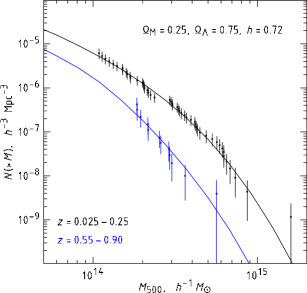
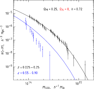
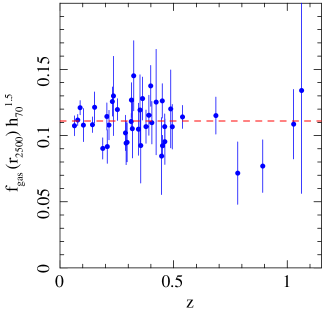
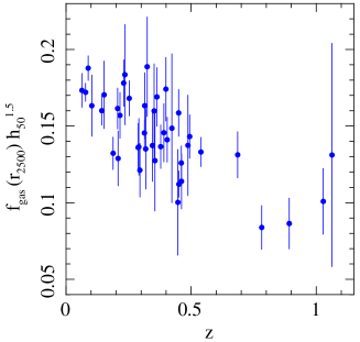
Figure 9: Examples of cluster data used in recent cosmological work. Top: Measured mass functions of clusters at low and high redshifts are compared with predictions of a flat, $\Lambda$CDM model and an open model without dark energy (from Vikhlinin et al. 2009b). Bottom: $f_{\mathrm{gas}}(z)$ measurements for relaxed clusters are compared for a $\Omega_{\mathrm{m}}=0.3$, $\Omega_{\Lambda}=0.7$, $h=0.7$ model (left, consistent with the expectation of no evolution) and a $\Omega_{\mathrm{m}}=1.0$, $\Omega_{\Lambda}=0.0$, $h=0.5$ model (right; from Allen et al. 2008). For purposes of illustration, cosmology-dependent derived quantities are shown (mass and $f_{\mathrm{gas}}$); in practice, model predictions are compared with cosmology-independent measurements.

The optically selected maxBCG sample (Koester et al. 2007) employed by Rozo et al. (2010) probes a different part of the cluster population; it is restricted to lower redshifts than the X-ray samples described above ($0.1<z<0.3$), but extends to lower masses ($M_{500}>7\times 10^{13}\,M_{\odot}$). This lower effective mass limit, which changes less strongly with redshift compared to X-ray surveys, makes the maxBCG sample significantly larger than the others, with $>10^{4}$ clusters divided into 9 bins based on optical richness. Mean masses for 5 richness ranges were estimated through a weak gravitational lensing analysis of stacked clusters, providing information from which to constrain the richness–mass relation. The cosmological analysis accounts for the covariance between cluster counts in each richness bin and the mean lensing mass estimates.

The results obtained by these three groups on flat $\Lambda$CDM and constant $w$ models are summarized in Table 2. Note that, for the two works which fit $w$ models, the results on $\Omega_{\mathrm{m}}$ and $\sigma_{8}$ are dominated by the low-redshift data and so are not degraded noticeably by the introduction of $w$ as a free parameter; thus all three sets of constraints are directly comparable. The agreement between the different works, as well as others listed in Table 2, is encouraging; in particular, the close agreement in the constraints on $\sigma_{8}$ reflects the relatively recent convergence in cluster mass estimates using different techniques, and our improved understanding of the relevant systematics (Section 3.3; see also, e.g., Henry et al. 2009). Importantly, the concordance $\Lambda$CDM model provides an acceptable fit to the data in each case.

Table 2: Recent cosmological results from galaxy clusters^a,b

Referencec	Data	$\sigma_{8}$	$\Omega_{\mathrm{m}}$	$\Omega_{\mathrm{DE}}$	$w$	$h$
Local abundance and evolutiond
M10	X-ray	$0.82\pm 0.05$	$0.23\pm 0.04$	$1-\Omega_{\mathrm{m}}$	$-1.01\pm 0.20$
V09	X-ray	$0.81\pm 0.04$	$0.26\pm 0.08$	$1-\Omega_{\mathrm{m}}$	$-1.14\pm 0.21$
Local abundance only
R10	optical	$0.80\pm 0.07$	$0.28\pm 0.07$	$1-\Omega_{\mathrm{m}}$	$-1$
H09	X-ray	$0.88\pm 0.04$	$0.3$	$1-\Omega_{\mathrm{m}}$	$-1$
Local abundance and clustering
S03	X-ray	$0.71^{+0.13}_{-0.16}$	$0.34^{+0.09}_{-0.08}$	$1-\Omega_{\mathrm{m}}$	$-1$
Gas-mass fraction
A08	X-ray		$0.27\pm 0.06$	$0.86\pm 0.19$	$-1$
A08	X-ray		$0.28\pm 0.06$	$1-\Omega_{\mathrm{m}}$	$-1.14^{+0.27}_{-0.35}$
E09	X-ray		$0.32\pm 0.05$	$1-\Omega_{\mathrm{m}}$	$-1.1^{+0.7}_{-0.6}$
L06	X-ray+SZ		$0.40^{+0.28}_{-0.20}$	$1-\Omega_{\mathrm{m}}$	$-1$
XSZ distances
B06	X-ray+SZ		$0.3$	$1-\Omega_{\mathrm{m}}$	$-1$	$0.77^{+0.11}_{-0.09}$
S04	X-ray+SZ		$0.3$	$1-\Omega_{\mathrm{m}}$	$-1$	$0.69\pm 0.08$

^a Entries $\Omega_{\mathrm{DE}}=1-\Omega_{\mathrm{m}}$ indicate the assumption of global spatial flatness (or use of WMAP priors requiring flatness at the few percent level); other entries without error bars indicate parameters that were fixed in the corresponding analysis.

^b Error bars are marginalized (single-parameter) 68.3% confidence intervals, and include each author’s estimate of the systematic uncertainties (with the exception of S04).

^c A08 = Allen et al. (2008); B06 = Bonamente et al. (2006); E09 = Ettori et al. (2009); H09 = Henry et al. (2009); L06 = LaRoque et al. (2006); M10 = Mantz et al. (2010b); R10 = Rozo et al. (2010); S03 = Schuecker et al. (2003); S04 = Schmidt, Allen & Fabian (2004); V09 = Vikhlinin et al. (2009b).

^d Cluster surveys extending to redshifts $z\ {\raise-3.22916pt\hbox{$\buildrel>\over{\sim}$}}\ 0.3$ are required to constrain $w$ from the evolution of the mass function. Note that the $\Omega_{\mathrm{m}}$ and $\sigma_{8}$ constraints from these works are essentially unchanged, whether or not $w$ is allowed to differ from $-1$.

Figure 10 (left panel) shows the joint constraints on $\Omega_{\mathrm{m}}$ and $\sigma_{8}$ obtained by Rozo et al. (2010, solid lines), which display the typical degeneracy between those parameters from cluster survey data. (The degeneracy can be broken, for example, by including cluster $f_{\mathrm{gas}}$ data; see Section 4.2.) Also shown are results from 5 years of WMAP data (Dunkley et al. 2009, dashed lines), which are tight for the assumed flat $\Lambda$CDM model. Nevertheless, it is evident that the combination of the two types of data (shaded regions) is significantly improved over either one individually.

      

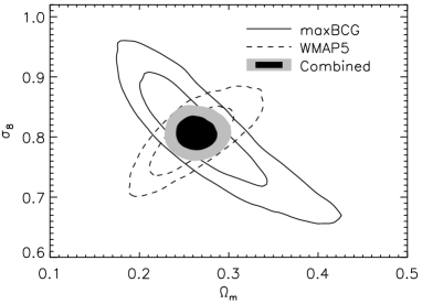
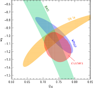
Figure 10: Left: Joint 68.3% and 95.4% confidence regions for the mean matter density and perturbation amplitude from the abundance of clusters in the maxBCG sample ($z<0.3$) compared with those from WMAP data (Dunkley et al. 2009) for spatially flat $\Lambda$CDM models. The shaded region indicates the combination of the two data sets. From Rozo et al. (2010). Right: Constraints on the dark energy density and equation of state from the abundance and growth of clusters in the 400 Square Degree sample ($z<0.9$) compared with those from WMAP, SNIa (Davis et al. 2007) and BAO (Eisenstein et al. 2005; Percival et al. 2007) for spatially flat, constant $w$ models. Note that, contrary to the convention followed in the other figures, the shaded regions in the right panel indicate only 39.3% confidence. The tight contraints from WMAP compared with Figure 11 result from the fact that a simplified analysis was used, in particular neglecting the influence of dark energy on the Integrated Sachs-Wolfe effect (e.g. Spergel et al. 2007). From Vikhlinin et al. (2009b).

The constraints on constant $w$ models from Vikhlinin et al. (2009b) and Mantz et al. (2010b) are respectively shown in Figures 10 (right panel) and 11, along with results from various other cosmological data sets. The cluster results are in good agreement with one another, as well as with the other, independent data. The $\sim 20\%$ precision constraint on $w$ from cluster growth alone (including systematic uncertainties) is clearly competitive, and further constraining power may be available from theoretical advances (see Section 4.5). The strong degeneracy in CMB constraints evident in Figure 11 also arises in many other models that are more complex than flat $\Lambda$CDM; the ability of cluster data to break this degeneracy by providing precise and independent constraints on $\sigma_{8}$ (right panel of Figure 11) makes the combination particularly powerful (e.g. Section 5.3).

      

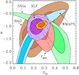
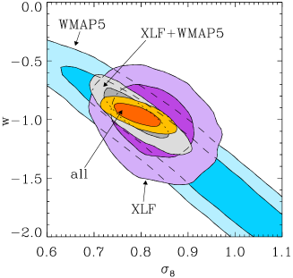
Figure 11: Joint 68.3% and 95.4% confidence regions for the dark energy equation of state and mean matter density (left) or perturbation amplitude (right) from the abundance and growth of RASS clusters at $z<0.5$ (labeled XLF; Mantz et al. 2010b) and $f_{\mathrm{gas}}$ measurements at $z<1.1$ (Allen et al. 2008), compared with those from WMAP (Dunkley et al. 2009), SNIa (Kowalski et al. 2008) and BAO (Percival et al. 2010) for spatially flat, constant $w$ models. Combined results from RASS clusters and WMAP are shown in gray in the right panel; gold contours in both panels show the combination of all data sets. The BAO-only constraint differs from that in Figure 10 due to the use of different priors. Adapted from Mantz et al. (2010b, the BAO constraints in the left panel have been updated to reflect more recent data).

Although their respective surveys are not yet complete, preliminary results have been reported from SZ-detected clusters from the South Pole Telescope (SPT; Vanderlinde et al. 2010) and Atacama Cosmology Telescope (ACT; Sehgal et al. 2011). As the number of cluster detections used in these works is small, respectively 21 and 9 at redshifts $0.16<z<1.2$, the data are not capable of producing interesting constraints on their own, but both groups demonstrate consistency with results from the WMAP satellite (Komatsu et al. 2011). Neither group has yet obtained simultaneous constraints on cosmology and the relevant SZ scaling relation, making their final error budgets strongly dependent on the priors chosen to constrain the scaling relation.

4.1.3 SCALING RELATIONS

To obtain scaling relations appropriate for constraining cosmology, the analysis of the two must be simultaneous and must account properly for the influence of the survey selection function (e.g. Stanek et al. 2006 and Sahlén et al. 2009) and the cluster mass function, as in Mantz et al. (2010a, see also Sections 4.1.1 and Section 2.5.1). Some authors have included corrections for the expected Malmquist bias given a flux limit or selection function (Pacaud et al. 2007; Pratt et al. 2009; Vikhlinin et al. 2009a), but most analyses of scaling relations in the literature employs least-squares regression without detailed consideration of sample selection. Since various cluster samples, with different selection functions, have been used, it is not surprising that results on the slopes, scatters and evolution of the scaling relations have varied widely compared with the formal uncertainties. Another statistical issue is that the covariance that comes about when the scaling quantities are measured from the same observations, for example temperature and hydrostatic masses from X-ray data, is commonly ignored (see Section 7).

The method used to estimate masses has also varied. Most authors have used the assumption of hydrostatic equilibrium applied to X-ray data, regardless of the dynamical state of the cluster, which must introduce spurious scatter due to departures from equilibrium and non-thermal support (e.g. Nagai, Vikhlinin & Kravtsov 2007). More recently, mass proxies such as gas mass (e.g. Mantz et al. 2010a) and X-ray thermal energy ($Y_{\mathrm{X}}$; e.g. Maughan 2007; Pratt et al. 2009; Vikhlinin et al. 2009a; Andersson et al. 2010), or gravitational lensing signal (e.g. Hoekstra 2007; Johnston et al. 2007; Rykoff et al. 2008; Leauthaud et al. 2010; Okabe et al. 2010) have been employed.

These variations in mass estimation and analysis methods, in addition to changes to instrument calibration over the years, makes a comprehensive and fair census of scaling relation results problematic. Here we focus on the cosmological importance of scaling relation measurements, citing examples from recent work where the issues mentioned above are at least partially mitigated.

For X-ray and SZ observables, under the assumption of strict self-similarity (no additional heating or cooling), Kaiser (1986) derived specific slopes and redshift dependences for the power-law form of Equation 16:

$$\frac{L_{\mathrm{bol}}}{E(z)} \propto \left[E(z)M\right]^{4/3},$$

$$kT_{\mathrm{mw}} \propto \left[E(z)M\right]^{2/3},$$

$$E(z)\,Y \propto \left[E(z)M\right]^{5/3},$$ (24)

where the factors of $E(z)=H(z)/H_{0}$ are appropriate for measurements made at a fixed critical-overdensity radius. The subscripts ‘bol’ and ‘mw’ reflect the fact that these predictions apply to the bolometric luminosity and mass-weighted temperature. Optical richness is more complex to predict, but empirical studies that map galaxies to sub-halos in simulations support a power law richness–mass relation for groups and clusters (Conroy & Wechsler 2009).

Figures 12 and 13 show a few examples of recent scaling relation measurements. Leauthaud et al. (2010) present a $M$–$L_{\mathrm{X}}$ relation for X-ray selected clusters in the COSMOS field by measuring stacked weak lensing masses (left panel of Figure 12). Under the common assumption of symmetric scatter in the log, stacking on $L_{\mathrm{X}}$ allows the mean $M(L_{\mathrm{X}})$ relation to be recovered, at the cost of losing information about the intrinsic scatter. As the authors note, transforming these results to an $L_{\mathrm{X}}(M)$ relation introduces a dependence on the mass function. Stacked lensing was also used to determine the mass–richness relation of optically selected clusters in SDSS by Johnston et al. (2007). Their results are shown in the right panel of Figure 12; red points in the figure show that compatible masses were derived from galaxy velocity dispersion measurements.

      

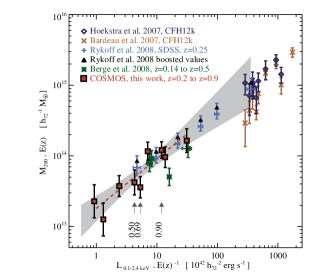
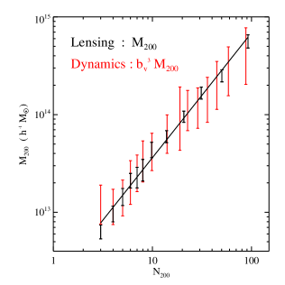
Figure 12: Scaling relations using masses from stacked weak lensing observations. The vertical axes show mean mass derived from stacking clusters in each bin. Left: X-ray selected clusters from the COSMOS field binned in luminosity (from Leauthaud et al. 2010, see references therein for other data sets plotted). The gray band corresponds to a 68% confidence predictive region from a fit to the COSMOS data (brown squares). Right: Optically selected clusters from SDSS (a subset of the maxBCG catalog) binned in richness. Black points are masses from weak lensing, while red points show mass determinations from galaxy velocity dispersion measurements for the same clusters (Becker et al. 2007). From Johnston et al. (2007).

For more massive systems, lensing can provide mass estimates on a cluster-by-cluster basis. The left panel of Figure 13 shows such a mass–temperature relation from Hoekstra (2007) for X-ray selected clusters. Since temperature only weakly influences X-ray detectability, selection bias should be relatively unimportant here, although intrinsic correlation with luminosity can still produces subtle biases relative to a mass-limited sample (Section 2.5.1).

      

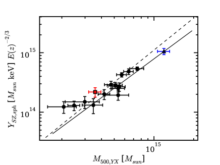
Figure 13: Scaling relations using masses estimated for individual clusters. Left: weak lensing masses versus ICM temperature for an X-ray selected sample imaged by the Canada–France–Hawaii Telescope. From Hoekstra (2007). Right: spherically-integrated SZ signal ($Y$) versus mass for SPT-detected clusters, where masses are estimated using X-ray thermal energy ($Y_{\mathrm{X}}$) from Chandra observations as a proxy. $Y$ is measured from the SPT survey data. The solid line is a fit to the data, while the dashed line shows a prediction based on the results of Arnaud et al. (2010). From Andersson et al. (2010).

An SZ scaling relation from Andersson et al. (2010), using clusters detected by SPT, appears in the right panel of Figure 13; in this case, masses are estimated from measurements of the X-ray thermal energy, $Y_{\mathrm{X}}$, and an assumed $Y_{\mathrm{X}}$–$M$ relation. This case is instructive in that the plotted $Y$ values are derived from the survey data, with suggestions of Malmquist bias in the flattening observed at the lowest masses (compare with Figure 5; this potential bias is accounted for in the fit in Figure 13).

Recently, the Planck Collaboration released an early SZ-selected cluster catalog together with an analysis of SZ scalings for existing X-ray and optical cluster samples (Planck Collaboration 2011a, and references therein). Measurements of the scaled SZ signal from Planck as a function of X-ray luminosity for $\sim 1600$ X-ray selected galaxy clusters are shown in the left panel of Figure 14, along with the stacked, mean SZ signal in luminosity bins and model expectations derived from the observed X-ray properties (Planck Collaboration 2011c). There is good agreement between the model expectations and the Planck observations, validating the simple model description of the hot ICM over the mass and redshift range probed.

      

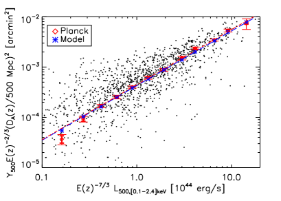
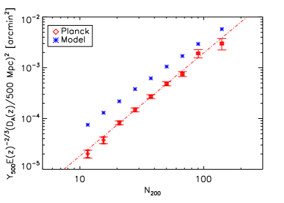
Figure 14: Recent SZ scaling relations from Planck. Left: scaled, intrinsic SZ signal vs. X-ray luminosity for a sample of X-ray selected clusters, with SZ extraction radii determined from $L_{\mathrm{X}}$ (see Planck Collaboration 2011c for details). Red diamonds show the $L_{\mathrm{X}}$-stacked relation, while the blue asterisks show the predicted SZ signal based on X-ray scaling relations. For these clusters, the agreement of the model with measurements is good. Right: Scaled, stacked SZ signal vs. optical richness for optically selected maxBCG clusters (red diamonds) are compared to expectations based on the maxBCG mass–richness relation in combination with X-ray scaling relations (blue asterisks, see Planck Collaboration 2011b for details). The origin of the offset between the predictions and measurements is not yet understood.

The right panel of Figure 14 shows the result of a similar exercise, stacking the Planck SZ signal as a function of richness for the optically selected maxBCG catalog. Also shown is the expected signal, based on the observed mean mass–richness relation for the maxBCG sample (Rozo et al. 2009) and a standard X-ray $Y$–$M$ scaling relation (Planck Collaboration 2011b). In this case, the observed Planck SZ signal lies well below model predictions. For an X-ray detected sub-sample of the maxBCG catalog, however, relatively good agreement between the Planck SZ measurements and model predictions is observed (Planck Collaboration 2011b).

An important difference between the $L_{\mathrm{X}}$ and richness comparisons is that the centers and radii used to extract the clusters’ SZ signals from the (relatively low resolution) Planck data were respectively based on X-ray and optical estimates. Besides optical center and scale mis-estimates, other potential sources for the discrepancy in Figure 14b include lower than expected purity in the optical sample (with lower mass halos being enhanced in richness by projection); unmodeled biases in the scaling relations used (e.g. the impact of non-thermal pressure support on the X-ray relations); and the presence of an intrinsic anti-correlation between the galactic and hot gas mass fractions in the clusters. These and other possibilities are under investigation.

In general, most current scaling results are consistent with power-law relations over a wide range in mass (e.g. Sun et al. 2009; Rozo et al. 2010). However, the exponents often differ from the values in Equation 4.1.3, due at least in part to the impact of astrophysical processes, mainly star/SMBH formation and associated feedback, discussed in Section 2.1.2. For example, the $L_{\mathrm{X}}$–$M$ slope is commonly found to exceed $4/3$, with the value depending on the mass range explored. There is less consensus on the $T_{\mathrm{X}}$–$M$ slope, with most estimates consistent with self-similarity (e.g. Henry et al. 2009; $m_{T}=0.65\pm 0.03$), but some finding a shallower slope (e.g. Mantz et al. 2010a; $m_{T}=0.48\pm 0.04$); systematics related to correlated observables, mass estimation (see Section 7), instrument calibration, selection, and differences in the mass range studied may play a role. There are fewer empirical estimates of the $Y$–$M$ or $Y_{\mathrm{X}}$–$M$ slopes, but most are broadly compatible with the predicted value. We note that departure from self-similar scaling with mass does not necessarily imply departure from self-similar evolution with redshift; for example, the high-mass halos in the preheated simulations of Stanek et al. (2010) have X-ray luminosities that evolve within $10\%$ of the self-similar expectation at $z\leq 1$, despite having a slope with mass that is $50\%$ steeper than self-similar.

The marginal intrinsic scatter in each relation determines the degree of selection bias in surveys and each observable’s usefulness as a mass proxy; current results are reviewed in Section 3.3.4.

The evolution of the scaling relations is of great importance, since it is potentially degenerate with the cosmological signal of cluster growth. Because the impact of survey limits can vary strongly with redshift for X-ray surveys, it is particularly crucial to account for them in this context. Both Vikhlinin et al. (2009a) and Mantz et al. (2010a) investigate evolution in the $L_{\mathrm{X}}$–$M$ relation, finding only marginal $\sim 1\sigma$ departures from the self-similar redshift dependence in Equation 4.1.3. Mantz et al. (2010a) additionally found no evidence for departures from self-similar evolution in the $T_{\mathrm{X}}$–$M$ or center-excised $L_{\mathrm{X}}$–$M$ relations (see Section 6.4). As current and upcoming surveys expand the reach of cluster samples to $z>1$, obtaining precise constraints on scaling relation evolution will be imperative (see also Section 7).

The effects of survey bias on scaling relations can be partially mitigated by selecting clusters based on an observable other than the observable of immediate interest (e.g. Rykoff et al. 2008). However, as Sections 2.4.1 and 2.5.1 make clear, the amount of residual bias depends on the intrinsic correlation between the two observables at fixed mass. To date, the only empirical estimates of such correlation are for mass and X-ray luminosity at fixed optical richness, $r(L_{\mathrm{X}},M|\hbox{$N_{\rm gal}$})\geq 0.85$ (Rozo et al. 2009); and for soft-band X-ray luminosity and temperature at fixed mass, $r(L_{\mathrm{X}},T_{\mathrm{X}}|M)=0.09\pm 0.19$ (Mantz et al. 2010a). Large, overlapping surveys, and/or surveys coupled with multi-wavelength follow-up campaigns, are required to better constrain the property covariance of clusters; ultimately, such constraints will provide a new level of robustness to cosmological work.

4.1.4 MOST MASSIVE CLUSTER TESTS

In principle, the confirmed existence of even a single galaxy cluster of implausibly high mass would challenge the standard $\Lambda$CDM model with Gaussian initial conditions. Recently, the discovery of high redshift, massive systems such as XMMU J2235.3-2557 at $z\sim 1.4$ (Mullis et al. 2005; Rosati et al. 2009) and SPT-CL J0546-5345 at $z\sim 1.1.$ (Brodwin et al. 2010) have led to reports of possible tension with Gaussian $\Lambda$CDM (Jee et al. 2009; Holz & Perlmutter 2010; Hoyle, Jimenez & Verde 2010).

Such a test is in some sense an attractively simple alternative to the more involved work discussed above. However, despite the fact that the test involves only one or a few very massive clusters detected in a survey rather than the complete sample, a robust assessment of the likelihood still requires a detailed understanding of the selection function and survey biases, as well as a full accounting for the effects of scatter in the mass–observable scaling relations (Sections 2.5.1 and 4.1.1). The accuracy and precision of the cluster mass measurements are also critical, due to the steepness of the high mass tail of the cluster mass function. Errors in mass measurements at the tens of per cent level, for example (as might be expected for weak lensing measurements of an individual cluster), can modify the likelihood of such a cluster being observed by up to an order of magnitude.

Mortonson, Hu & Huterer (2011) estimate confidence limits for the exclusion of the Gaussian $\Lambda$CDM model based on the properties of the most massive galaxy cluster, or $N$ most massive galaxy clusters, detected in a given survey, employing constraints on the expansion history from current data. These authors conclude that none of the presently known high mass, high redshift clusters are in significant tension with the standard Gaussian $\Lambda$CDM paradigm.

4.1.5 CLUSTERING

The framework described in Section 4.1.1 for simultaneously constraining cosmology and scaling relations has yet to be applied to the spatial clustering of clusters. However, Schuecker et al. (2002) have obtained cosmological constraints using a method based on the Karhunen-Loève eigenvectors of 428 clusters from the X-ray selected REFLEX sample above a luminosity of $5.1\times 10^{42}h_{70}^{-2}\mathrm{\,erg}\mathrm{\,s}^{-1}$ (see Vogeley & Szalay 1996 for the theory underlying this method of estimating the power spectrum). The constraints are relatively weak compared with more recent results from other methods: $0.6<\sigma_{8}<2.6$ and $0.07<\Omega_{\mathrm{m}}<0.38$ at 95.4% confidence, fixing $h=0.7$ and without including the systematic uncertainty due to cosmic variance. In Schuecker et al. (2003), the analysis was extended to include cluster abundance using an empirical X-ray luminosity–mass scaling relation from Reiprich & Böhringer (2002), demonstrating that the combination of the two methods breaks the degeneracy between $\Omega_{\mathrm{m}}$ and $\sigma_{8}$, in particular reducing the uncertainty on $\sigma_{8}$ to the point where systematics related to mass estimation dominate (Table 2).

In principle, the spatial distribution of clusters can be employed in a simpler way, as has been done with individual galaxies, by using the baryon acoustic oscillation signature in the power spectrum as a probe of cosmic distance. Estrada, Sefusatti & Frieman (2009) and Hütsi (2010) respectively analyzed the correlation function and power spectrum of clusters in the optically selected maxBCG catalog, finding a weak ($\sim 2\sigma$) detection of the BAO peak. More recently, Balaguera-Antolínez et al. (2011) found no significant evidence for a BAO feature in the smaller, X-ray selected REFLEX II catalog.

4.2 Baryon Fractions

Cluster gas mass fractions can be measured robustly using X-ray, or the combination of X-ray and SZ, data for dynamically relaxed clusters (Section 3). When measured from X-ray data, $f_{\mathrm{gas}}$ values within a given angular aperture depend on cosmology as $f_{\mathrm{gas}}(z)\propto d_{\mathrm{A}}(z)^{3/2}$, while the predicted $f_{\mathrm{gas}}$ for a given cosmology is given by Equation 10. (A more detailed expression for the comparison of measured and predicted $f_{\mathrm{gas}}$ values is given by Allen et al. 2008, who include terms accounting for instrument calibration, non-thermal pressure, and the relationship between the characteristic radius of the model, e.g. $r_{2500}$, and the aperture of the measurement.) The apparent redshift dependence of $f_{\mathrm{gas}}$ measurements on the cosmological background is illustrated in the bottom panels of Figure 9.

In principle, $f_{\mathrm{gas}}$ measurements can be made at radii corresponding to any overdensity. In practice, this overdensity should be low enough (i.e. the radius large enough) that non-gravitational feedback effects do not introduce prohibitive scatter; but not so small (i.e. the radius not so large) that the measurements become dominated by the systematic limitations of the instruments. A variety of simulations indicate that radii $\sim r_{2500}$ are sufficiently large to benefit from low $f_{\mathrm{gas}}$ scatter (e.g. Borgani & Kravtsov 2011), while at radii $\ {\raise-3.22916pt\hbox{$\buildrel>\over{\sim}$}}\ r_{500}$ uncertainties in the X-ray background and the impact of gas clumping can become a concern (Simionescu et al. 2011; see also Section 6.3).

Using this method, Allen et al. (2008, see also ) obtained cosmological constraints using $f_{\mathrm{gas}}$ measurements at $r_{2500}$ from Chandra observations of 42 hot ($kT_{\mathrm{X}}>5\mathrm{\,keV}$), relaxed clusters covering the redshift range $0.05<z<1.1$. Their analysis incorporated weak priors on $h$ and $\Omega_{\mathrm{b}}h^{2}$ from Hubble Key Project (Freedman et al. 2001) and big bang nucleosynthesis data, priors on the baryonic depletion and stellar mass fraction of clusters and their evolution (the term $\Upsilon(z)$ in Equation 10), and marginalized over systematic allowances accounting for instrument calibration and non-thermal pressure. From Equation 10, we see that the normalization of the $f_{\mathrm{gas}}(z)$ curve, combined with the priors on $h$ and $\Omega_{\mathrm{b}}h^{2}$, provides a constraint on $\Omega_{\mathrm{m}}$; while the shape of $f_{\mathrm{gas}}(z)$ allows dark energy parameters to be constrained via the apparent dependence of $f_{\mathrm{gas}}$ on distance. The results for spatially flat, constant $w$ models and non-flat $\Lambda$CDM models are respectively shown in Figures 11 and 15. For the non-flat models, the presence of dark energy is detected at high ($>99.99\%$) confidence, comparable to current SNIa results; the constraints, including systematic uncertainties, are $\Omega_{\mathrm{m}}=0.27\pm 0.06$ and $\Omega_{\Lambda}=0.86\pm 0.19$, with the flat $\Lambda$CDM model yielding an acceptable goodness of fit. For constant $w$ models, the $f_{\mathrm{gas}}$ data are again competitive with other cosmological results, obtaining $w=-1.14^{+0.27}_{-0.35}$. The systematic, cluster-to-cluster scatter in $f_{\mathrm{gas}}$ is small, $<7\%$, corresponding to only 5% in distance; this high precision results from the restriction to hot, dynamically relaxed systems for which total masses can be accurately estimated (Section 3.3.1).

Interestingly, for clusters with $kT\ {\raise-3.22916pt\hbox{$\buildrel>\over{\sim}$}}\ 5\mathrm{\,keV}$, the measured $f_{\mathrm{gas}}$ values show no dependence on temperature (right panel of Figure 15), indicating that, for the most massive clusters, the self-similar expectation of constant $f_{\mathrm{gas}}$ with mass is realized. At lower temperature and mass (extending to the group scale), a trend of increasing $f_{\mathrm{gas}}$ with temperature and mass is observed (e.g. Sun et al. 2009).

      

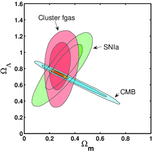
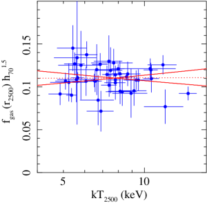
Figure 15: Left: Joint 68.3% and 95.4% confidence regions on $\Lambda$CDM models with curvature from cluster $f_{\mathrm{gas}}$ data at $z<1.1$, compared with those from CMB data (Spergel et al. 2007) and SNIa (Davis et al. 2007). Inner, gold contours show results from the combination of these data. Right: $f_{\mathrm{gas}}$ values as a function of ICM temperature. The measurements are consistent with a constant value over the temperature range explored ($5\mathrm{\,keV}<kT_{\mathrm{X}}<15\mathrm{\,keV}$). From Allen et al. (2008).

Ettori et al. (2009) have also applied X-ray data to the $f_{\mathrm{gas}}$ test, using Chandra measurements at $r_{500}$ for 52 clusters in the redshift range $0.3<z<1.3$, adopting similar priors on $h$ and $\Omega_{\mathrm{b}}h^{2}$ and marginalizing over a prior on $\Upsilon$ (assumed constant with redshift). However, their data set was not restricted to dynamically relaxed systems, resulting in significantly weaker constraints (Table 2).

LaRoque et al. (2006) employed Chandra X-ray and OVRO/BIMA SZ observations of 38 clusters in the redshift range $0.14<z<0.89$ (with no restriction dynamically relaxed systems), finding $f_{\mathrm{gas}}$ values consistent with previous X-ray work. (Their analysis did not take advantage of the relative normalization of the X-ray and SZ signals to simultaneously provide a second distance constraint; see Section 4.3.) They adopted the simpler approach of assuming constant $f_{\mathrm{gas}}$ and marginalizing over its value, incorporating a WMAP prior on the total density, $\Omega_{\mathrm{m}}+\Omega_{\Lambda}$. Although this explicitly ignores the information available from the normalization of $f_{\mathrm{gas}}(z)$, their results clearly disfavor a dark matter dominated universe, preferring a low-density universe with dark energy (Table 2).

4.3 XSZ Distances

The different dependence on distance of the gas density inferred from X-ray and SZ observations of clusters can be exploited in a conceptually similar way to $f_{\mathrm{gas}}$ data (Section 2.2.3). The most recent contribution is that of Bonamente et al. (2006), who measured distances to 38 clusters at redshifts $0.14<z<0.89$. This cosmological test is intrinsically less sensitive to distance than the $f_{\mathrm{gas}}$ test, with the signal proportional only to $d_{\mathrm{A}}(z)^{1/2}$ (Equation 11), and currently can constrain only one free parameter. Assuming spatial flatness and fixing $\Omega_{\mathrm{m}}=0.3$, Bonamente et al. (2006) obtained a constraint on the Hubble parameter, $h=0.77^{+0.11}_{-0.09}$, consistent with results from other data such as the Hubble Key Project (Freedman et al. 2001) or the combination of $f_{\mathrm{gas}}$ and CMB data (Allen et al. 2008). We note that other works using the same method have typically found somewhat lower best fitting values ($h=0.6$–0.7; e.g. Grainge et al. 2002; Schmidt, Allen & Fabian 2004), but these discrepancies are not significant given the systematic uncertainties.

4.4 High-Multipole CMB Power Spectrum

The CMB temperature power spectrum at multipoles $\ell\ {\raise-3.22916pt\hbox{$\buildrel>\over{\sim}$}}\ 1000$ encodes the thermal SZ signature of unresolved clusters at all masses and redshifts (Section 2.2.4). Although the primary CMB power decreases rapidly at these scales, extracting this cosmological information from the tSZ spectrum has proved challenging due to uncertainties in, e.g., the relevant observable–mass scaling relation at low masses and high redshifts; the population of infrared and radio point sources; the magnitude of the integrated kinetic SZ effect; and the form of the electron pressure profile at large cluster radii, where it is poorly constrained by current X-ray data (Sehgal et al. 2010; Section 6.3). The WMAP, SPT and ACT collaborations have all detected excess power at large multipoles, $\ell\ {\raise-3.22916pt\hbox{$\buildrel>\over{\sim}$}}\ 3000$. Subject to the systematic uncertainties mentioned, their results are broadly in agreement, and are consistent with estimates of $\sigma_{8}$ obtained from studies of resolved clusters and the primary CMB (Dunkley et al. 2010; Lueker et al. 2010; Komatsu et al. 2011).

4.5 Evolving Dark Energy Models

As discussed above, current cluster growth and $f_{\mathrm{gas}}$ data can constrain spatially flat models with constant $w$, finding consistency with the cosmological constant model ($w=-1$). Constraints on constant $w$ models from the combination of these cluster data are shown in the left panel of Figure 16. To go beyond this simple description of dark energy, it is necessary to include cosmological data from additional sources in the analysis.

      

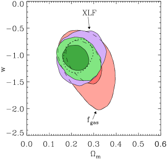
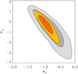
Figure 16: Left: Joint 68.3% and 95.4% confidence regions for constant $w$ models, using cluster growth (XLF; Mantz et al. 2010b) and $f_{\mathrm{gas}}$ (Allen et al. 2008) data and their combination (green contours). These cluster data provide a $15\%$ precision constraint on $w$ ($w=-1.06\pm 0.15$) without incorporating CMB, SNIa or BAO data. Right: Constraints on parameters of the evolving $w$ dark energy model in Equation 6 from the combination of cluster growth and WMAP (Dunkley et al. 2009) data (gray), and with the addition of cluster $f_{\mathrm{gas}}$, SNIa (Kowalski et al. 2008) and BAO (Percival et al. 2007) data (gold). The $\Lambda$CDM model ($w(z)=-1$) corresponds to the black cross. From Mantz et al. (2010b).

Equation 6 provides a simple and commonly adopted model of evolving dark energy, in which the equation of state takes the value $w_{0}$ at $z=0$ and approaches $w_{0}+w_{a}$ at high redshift. Constraints on this model were obtained from cluster growth data by Vikhlinin et al. (2009b) and Mantz et al. (2010b), assuming spatial flatness and in combination with external CMB, SNIa and BAO (and $f_{\mathrm{gas}}$, in the case of Mantz et al.) data. In both studies, the results are consistent with the $\Lambda$CDM model ($w_{0}=-1$ and $w_{a}=0$; right panel of Figure 16).

A slightly more general model due to Rapetti, Allen & Weller (2005),

$$w(z)=\frac{w_{\mathrm{et}}z+w_{0}z_{\mathrm{t}}}{z+z_{\mathrm{t}}},$$ (25)

also makes a smooth transition from one value at the present day ($w_{0}$) to another at early times ($w_{\mathrm{et}}$), but has the advantage that the transition redshift, $z_{\mathrm{t}}$, can be marginalized over. (When $z_{\mathrm{t}}=1$, Equation 25 reduces to Equation 6 with $w_{a}=w_{\mathrm{et}}-w_{0}$.) Mantz et al. (2010b) used the data sets above to obtain $w_{0}=-0.88\pm 0.21$ and $w_{\mathrm{et}}=-1.05^{+0.20}_{-0.36}$, again consistent with $\Lambda$CDM.

Absent a concrete physical model for dark energy, phenomenological models of evolving dark energy can take any form; for example, one possibility that has not yet been investigated using cluster data expands $w(z)$ in principal components (e.g. Mortonson, Hu & Huterer 2010). Although these ad-hoc descriptions of dark energy are perfectly straightforward to apply to measurements of the expansion history, their applicability to an analysis based on the cluster mass function or power spectrum is less clear. Generically, descriptions of dark energy as a fluid with $w\neq-1$ should include the effects of spatial variations in dark energy density (e.g. Hu 2005). However, the results from cluster growth so far have made use of mass functions from $\Lambda$CDM simulations, accounting for the value of $w$ only in the expansion history (Vikhlinin et al. 2009b) or, at most, including the effect of density variations on the linear matter power spectrum (Mantz et al. 2008, 2010b). In principle, the cluster mass function must also be adjusted to account for the behavior of fluid dark energy on smaller scales and in higher density environments. Encouragingly, preliminary work in this area suggests that the influence of dark energy on the mass function might be readily measurable, resulting in additional constraining power from clusters (e.g. Creminelli et al. 2010). Such improvements, however, might come at the cost of requiring additional sophistication in the theoretical description of dark energy (e.g. the dark energy sound speed and viscosity; Mota et al. 2007).

5 OTHER CONTRIBUTIONS TO FUNDAMENTAL PHYSICS

5.1 Dark Matter

The $\Lambda$CDM paradigm, while providing an excellent model for the large scale structure of the Universe, incorporates little information on the physical nature of dark matter. It assumes only that dark matter is non-baryonic; that it interacts weakly with baryonic matter and itself; that it emits and absorbs no detectable electromagnetic radiation; and that the dark matter particles move at sub-relativistic speeds.

As clusters merge under the pull of gravity, their dark matter halos and X-ray emitting gas can become separated temporarily, as the gas experiences ram pressure and is slowed. The observed offsets between the dark matter and X-ray peaks in the Bullet Cluster (1E 0657-558; Bradač et al. 2006; Clowe et al. 2006) and MACS J0025.4-1222 (Bradač et al. 2008a; Figure 17), both massive merging systems with relatively simple geometries, require conservatively that the scattering depth for the merging dark matter cannot be greater than one. Using gravitational lensing data to estimate the dark matter column densities through these clusters, Markevitch et al. (2004) and Bradač et al. (2008a) use the observed dark matter and X-ray peak separations to derive limits on the velocity-independent dark matter self-interaction cross-section per unit mass of $\sigma/m<5$ cm² g^-1 and $\sigma/m<4$ cm² g^-1 for 1E 0657-558 and MACS J0025.4-1222, respectively. Randall et al. (2008) additionally use the non-detection of an offset between the lensing peaks and the galaxy centroids for the Bullet Cluster to refine this constraint to $\sigma/m<1.5$ cm² g^-1. Upcoming surveys (Section 6.1), should provide hundreds of similar examples, removing the current systematic limitations set by small number statistics. In combination with multiwavelength follow-up observations and improved numerical simulations (e.g. Forero-Romero, Gottlöber & Yepes 2010), this should allow the properties of dark matter in merging clusters to be studied in a robust, statistical manner.

One of the most remarkable predictions of the CDM model is that the density profiles of relaxed dark matter halos, on all resolvable mass scales, can be approximated by a simple, universal profile (Equation 15) with an inner, density slope $\rho_{\rm DM}\ {\raise-3.22916pt\hbox{$\buildrel\propto\over{\sim}$}}\ r^{-1}$. In contrast, for dark matter models with significant self-interaction cross sections, halos are expected to exhibit flattened, quasi-isothermal cores (Spergel & Steinhardt 2000; Yoshida et al. 2000). In the absence of significant rotational support, these cores are also expected to be approximately spherical.

Using Chandra X-ray data for a sample of massive, dynamically relaxed galaxy clusters, Schmidt & Allen (2007) measure a mean central density slope of $-0.88\pm 0.29$ (95 per cent confidence limits), in good agreement with $\Lambda$CDM. Detailed strong-plus-weak lensing analyses for a subset of these systems yields consistent constraints (Bradač et al. 2008b; Newman et al. 2009, 2011). On smaller scales, using stellar velocity dispersion profiles for the dominant cluster galaxies, Sand et al. (2008) (see also Newman et al. 2011) infer a possible flattening of the central dark matter halos in Abell 383 and MS 2137.3-2353. However, on these small scales, the impact of baryonic physics becomes important.

Arabadjis, Bautz & Garmire (2002) use the lack of a dark matter core in X-ray and lensing data for the relaxed cluster MS 1358+6245, to place a limit on the velocity independent dark matter particle-scattering cross section $\sigma/m<0.1$ cm² g^-1. Miralda-Escudé (2002) use constraints on the ellipticity in the central regions of MS 2137.3-2353 to infer $\sigma/m<0.02$ cm² g^-1. To improve these constraints, combined multiwavelength observations for large samples of relaxed clusters, coupled with improved simulations modeling fully the interactions between dark matter and baryons, are required.

Certain dark matter candidates, including sterile neutrinos, possess a two-body radiative decay channel that produces a photon with energy $E_{\gamma}=M_{\rm DM}/2$, where $M_{\rm DM}$ is the dark matter particle mass (e.g. Feng 2010). Galaxy clusters have been the targets of searches for emission lines associated with such decays. The soft X-ray (keV) regime is particularly interesting, marking the lower limit of masses consistent with constraints from large scale structure formation. To date, all searches for monochromatic X-ray emission lines associated with non-baryonic matter in clusters (as well as other dark matter rich objects) have proved negative (e.g. Boyarsky et al. 2006; Riemer-Sorensen et al. 2007; Boyarsky, Ruchayskiy & Markevitch 2008). Gamma-ray observations of clusters with the Fermi Gamma-ray Space Telescope have been used to place interesting upper limits on dark matter annihilation, and the lifetimes of particles for a range of masses and decay final states (Ackermann et al. 2010; Dugger, Jeltema & Profumo 2010).

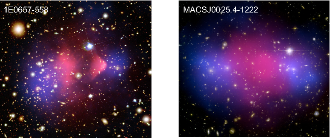
Figure 17: Hubble Space Telescope optical images of the massive, merging clusters 1E0657-558 ($z=0.30$) and MACSJ0025.4-1222 ($z=0.54$), with the X-ray emission measured with Chandra overlaid in pink and total mass reconstructions from gravitational lensing data in blue. The separations of the X-ray and lensing peaks, and the coincidence of the lensing and optical centroids, imply that the dark matter has a small self-interaction cross-section. Figure credits: Left: X-ray: NASA/CXC/CfA/M.Markevitch et al.; Optical: NASA/STScI; Magellan/U.Arizona/D.Clowe et al.; Lensing Map: NASA/STScI; ESO WFI; Magellan/U.Arizona/D.Clowe et al.; Right: X-ray: NASA/CXC/Stanford/S.Allen; Optical/Lensing: NASA/STScI/UC Santa Barbara/M.Bradač.

5.2 Gravity

Dark energy, though a key component of the standard cosmological model, provides by no means the only possible explanation for cosmic acceleration. Various non-standard gravity models can also produce acceleration on cosmological scales (for reviews, see Copeland, Sami & Tsujikawa 2006; Frieman, Turner & Huterer 2008). These include frameworks that consistently parametrize departures from General Relativity (GR; Hu & Sawicki 2007; Amin, Wagoner & Blandford 2008; Daniel et al. 2010); full, alternative theories such as the Dvali-Gabadadze-Porrati (DGP) braneworld gravity (Dvali, Gabadadze & Porrati 2000); $f(R)$ modifications of the Einstein-Hilbert action (Carroll et al. 2004); and modifications of gravity based on the mechanism of ghost condensation (Hamed et al. 2004). A critical requirement for any modified gravity model is that it should mimic GR in the relatively small scale, high density regime where GR has been tested precisely. Thus, in addition to investigating whether dark energy is well described by a cosmological constant, we are simultaneously interested in asking whether GR provides the correct description of gravity, and indeed whether dark energy is needed at all.

To discriminate among these possibilities, and between particular dark energy and modified gravity models, it is important to combine expansion history data with measurements of the growth and scale-dependence of cosmic structure. Galaxy clusters provide some of our strongest constraints on structure growth. To utilize these constraints robustly, however, accurate predictions for the halo mass function are required. Recently, a few mass functions for specific modified gravity models have been constructed and calibrated using N-body simulations. These include the self-accelerated branch (Chan & Scoccimarro 2009; Schmidt 2009b) and normal branch (Schmidt 2009a) of DGP gravity, and an $f(R)$ model (Schmidt et al. 2009). Constraints on the latter model using the observed local cluster abundance and other data are presented by Schmidt, Vikhlinin & Hu (2009).

An alternative to evaluating specific gravity theories is to adopt a convenient, parameterized description for the growth of structure. This can then be used to constrain departures from the predictions of $\Lambda$CDM+GR (Nesseris & Perivolaropoulos 2008). At late-times, the linear growth rate can be simply parametrized as (e.g. Linder 2005)

$$\frac{d\ln\delta}{d\ln a}=\Omega_{\mathrm{m}}(a)^{\gamma},$$ (26)

where $\delta$ is the density contrast and $\gamma$ the growth index. Conveniently, GR predicts a nearly constant and scale-independent value of $\gamma\approx 0.55$ for models consistent with current expansion data. As in the case of $w$ for dark energy models, constraining $\gamma$ constitutes a phenomenological approach to studying gravity. Rapetti et al. (2009, 2010) report constraints on departures from GR on cosmic scales using this parameterization with cluster data. Their results are simultaneously consistent with GR ($\gamma\sim 0.55$) and $\Lambda$CDM ($w=-1$) at the 68 per cent confidence level (left panel of Figure 18).

      

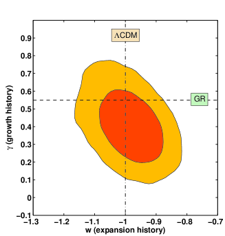
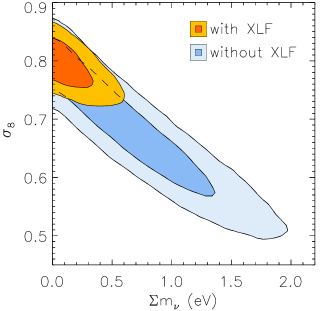
Figure 18: Left: Joint 68.3% and 95.4% confidence regions for departures from a General Relativistic growth history, parameterized by $\gamma$, and a $\Lambda$CDM expansion history, parameterized by $w$. The analysis uses a combination of cluster growth (XLF; Mantz et al. 2010b), $f_{\mathrm{gas}}$ (Allen et al. 2008), WMAP (Dunkley et al. 2009), SNIa (Kowalski et al. 2008) and BAO (Percival et al. 2007) data. From Rapetti et al. (2010). Right: Constraints on neutrino mass and the amplitude of density perturbations for $\Lambda$CDM models, including global curvature and marginalized over the amplitude and spectral index of primordial tensor perturbations. Gold contours correspond to the same combination of data as in the left panel; blue contours show the strong degeneracy between neutrino mass and $\sigma_{8}$ that exists when cluster growth data are not included in the analysis. From Mantz, Allen & Rapetti (2010).

5.3 Neutrinos

The mass of neutrinos directly influences the growth of cosmic structure, since any particle with non-zero mass at some point cools from a relativistic state, in which it effectively suppresses structure formation, to a non-relativistic state, in which it actively participates in the growth of structure (details are reviewed in Lesgourgues & Pastor 2006). In the standard scenerio where the neutrino species have approximately degenerate mass, the species-summed mass, $\sum m_{\nu}$, is sufficient to describe their cosmological effects.

Although current data lack the precision to directly detect the effect of neutrino mass on the time-dependent growth of clusters, cluster data do play a key role in cosmological constraints on neutrinos when combined with CMB observations. On its own, the CMB can place only a relatively weak upper bound on the mass, $\sum m_{\nu}<1.3\mathrm{\,eV}$ at 95% confidence for a $\Lambda$CDM model (e.g. Dunkley et al. 2009; works discussed here used 5 years of WMAP data, but their conclusions are not significantly changed by the 7-year update). Incorporating cosmic distance measurements improves this to $\sum m_{\nu}<0.61\mathrm{\,eV}$, with the results displaying a strong degeneracy between $\sum m_{\nu}$ and the value of $\sigma_{8}$ predicted from the amplitude of the primordial power spectrum, due to the integrated effect of neutrinos on the growth of structure. Cluster data at low redshift provide a direct measurement of $\sigma_{8}$, breaking this degeneracy (right panel of Figure 18), improving the upper limit by a further factor of two, to $\sum m_{\nu}<0.33\mathrm{\,eV}$ (Vikhlinin et al. 2009b; Mantz, Allen & Rapetti 2010; Reid et al. 2010). The degeneracy-breaking power of cluster observations also significantly improves the robustness of neutrino mass limits to the assumed cosmological model (e.g. marginalizing over global curvature; Mantz, Allen & Rapetti 2010; Reid et al. 2010). In combination with Planck data, expected near-term improvements in cluster mass measurements from high-quality lensing data could reduce the limit on $\sum m_{\nu}$ to the point of distinguishing between the normal and inverted neutrino mass hierarchies.

6 OPPORTUNITIES

6.1 Cluster Surveys on the Near and Mid-Term Horizons

In the near future (over the next 2–3 years), the completion of the SPT, ACT and Planck SZ catalogs will extend our detailed, statistical knowledge of galaxy clusters out to $z>1$. Together, these projects expect to find $\sim 1000$ new clusters, mostly at intermediate-to-high redshifts (Marriage et al. 2010; Vanderlinde et al. 2010). Used in combination with existing low-redshift X-ray and optical catalogs, they should provide significant improvements in our knowledge of cluster growth, and corresponding improvements in the constraints on dark energy and gravity models. As discussed in Section 3.2.3, challenges for these surveys will be defining and calibrating the optimal survey mass proxies, and understanding the impact of contamination from associated infrared sources and AGN. Looking further ahead, the development of experiments with improved spatial resolution, expanded frequency coverage and improved sensitivity, such as the Cerro Chajnantor Atacama Telescope (CCAT), will be of advantage.

At optical and near-infrared wavelengths, a suite of powerful, new ground-based surveys are about to come on-line. These include the Panoramic Survey Telescope and Rapid Response System (Pan-STARRS); the Dark Energy Survey (DES); the KIlo-Degree Survey (KIDS) and complementary VISTA Kilo-degree INfrared Galaxy survey (VIKING); the Subaru Hyper Suprime-Cam survey (HSC); and, later, the Large Synoptic Survey Telescope (LSST). These experiments offer significant potential for finding clusters, and will provide critical photometric redshift and lensing data. A primary challenge in constructing optical cluster catalogs will be the definition of robust mass proxies with minimal, well-understood scatter across the mass and redshift ranges of interest. Planned, space-based survey missions such as the Wide Field Infrared Survey Telescope (WFIRST) and Euclid also offer outstanding potential for cluster cosmology, complementing the ground-based surveys in providing lensing masses and photometric redshifts, and extending cluster search volumes out to higher redshifts.

In the near term, X-ray cluster samples constructed from serendipitous detections in Chandra and XMM-Newton observations offer the potential for important gains (e.g. Fassbender 2008; Sahlén et al. 2009). The main advances at X-ray wavelengths, however, will be provided by the eROSITA telescope on the Spektrum-Roentgen-Gamma Mission. Scheduled for launch in 2012, eROSITA will perform a four year all-sky survey that should detect an estimated 50,000–100,000 clusters with excellent purity and completeness. As discussed in Section 3.2.1, the unambiguous detection of clusters at X-ray wavelengths requires angular resolution to distinguish point sources from extended cluster emission. At modest redshifts and high fluxes, this should be straightforward for eROSITA; at high redshifts ($z>1$) and faint fluxes, however, separating cool-core clusters from AGN will be challenging and will require follow-up observations. Here, we note more than a dozen known examples of powerful AGN surrounded by X-ray bright clusters at intermediate-to-high redshifts (e.g. Belsole et al. 2007; Siemiginowska et al. 2010). Looking further ahead, the development of improved X-ray mirrors with high spatial resolution across a wide field of view, such as those proposed for the Wide Field X-ray Telescope, would be a major advance, rendering trivial the removal of contaminating AGN emission and allowing surveys to take full advantage of the center-excised X-ray luminosity as a low-scatter mass proxy (Section 6.4).

For all of these surveys, accurate calibration will be important; this is a particular challenge for space-based missions. In comparison to other cosmological probes, the demands on photo-$z$ calibration will be relatively modest. This is due both to the pronounced 4000 Å break in early-type galaxy spectra and the ability to combine measurements for many galaxies per cluster. Fisher matrix studies by Cunha, Huterer & Doré (2010) suggest targets of $<0.003$ for bias error and $<~{}0.03$ for error in the scatter in surveys with $\sim\!10^{5}$ clusters. For surveys with fewer counts, shot noise dominates, and photo-$z$ errors become less important.

Extensive programs of follow-up observations using high resolution, high throughput telescopes will also be essential. X-ray observatories like Chandra, XMM-Newton, Suzaku and ASTRO-H are likely to remain cornerstones of this work, providing excellent, low-scatter mass proxy measurements for individual clusters. We note that such information need only be gathered for a fraction of the clusters in a survey to gain a significant boost in constraining power with respect to self-calibration alone (e.g. Wu, Rozo & Wechsler 2010). Statistical calibration of the mean masses of clusters in flux and redshift intervals from weak lensing measurements will also be critical: in order for the intrinsic power of large surveys not to be impacted severely, calibration of the mean mass at the few per cent level is required (Wu, Rozo & Wechsler 2010). To achieve this accuracy, detailed redshift information for the lensed, background sources will be needed; indeed, the use of full redshift probability density functions rather than simple color cuts may be required. Detailed simulations will also be needed to probe the systematic limitations of these measurements, and to advise on the best analysis approaches (Section 6.5).

6.2 Footprints of Inflation: Primordial Non-Gaussianites

Inflation predicts a near scale invariant power spectrum and nearly Gaussian distribution for the primordial curvature inhomogeneities that seed LSS. For slow-roll, single-field inflation, departures from Gaussianity are currently unobservable (by at least four orders of magnitude; Acquaviva et al. 2003; Maldacena 2003). However, other multi-field and single-field inflation models predict observable non-Gaussianity (NG). Examples include certain brane models such as the Dirac-Born-Infeld (DBI) inflation; single-field models with non-trivial kinetic terms; ghost inflation; models in which density perturbations are generated by another field such as the curvaton; and models with varying inflation decay rate. (See Chen 2010 and Komatsu 2010 for recent reviews.) Any detection of NG would provide critical information about the physical processes taking place during inflation. In particular, a convincing detection of NG of the ‘local’ type (referring to particular configurations in Fourier space) would rule out not only slow-roll but all classes of single field inflation models (Creminelli & Zaldarriaga 2004).

Current measurements of CMB anisotropies and LSS are consistent with Gaussianity (Slosar et al. 2008; Komatsu et al. 2011). In principle, measurements of the clustering and abundance of galaxy clusters can also be used to place powerful, complementary constraints. Galaxy clusters trace the rare, high-mass tail of density perturbations in the Universe (Section 2) and are uniquely sensitive to NG. N-body simulations have been used to study cluster formation under non-Gaussian initial conditions (e.g. Desjacques, Seljak & Iliev 2009; Grossi et al. 2009; Pillepich, Porciani & Hahn 2010). Analytical mass functions have also been calculated using the Press-Schechter formalism (Lo Verde et al. 2008; D’Amico et al. 2011) or excursion set theory (Maggiore & Riotto 2010).

To date, CMB and LSS studies have only been used to place scale-independent constraints on NG. However, certain models that produce relatively large NG (see above) also present strong scale-dependence of the signal, due to, e.g., a changing (effective or otherwise) sound speed (Lo Verde et al. 2008). The addition of measurements at the smaller, galaxy cluster scale should provide important constraints on such models (Riotto & Sloth 2011; Shandera, Dalal & Huterer 2011). Several recent works (Oguri 2009; Cunha, Huterer & Doré 2010; Sartoris et al. 2010) have investigated quantitatively the potential of future optical and/or X-ray cluster surveys for constraining NG.

6.3 The Thermodynamics of Cluster Outskirts

To date, robust thermodynamic measurements have, in general, only been possible for the inner parts of clusters ($r\ {\raise-3.22916pt\hbox{$\buildrel<\over{\sim}$}}\ r_{500}$), where the X-ray emission is brightest and the SZ signal strongest; a large fraction of their volumes remain practically unexplored. Precise, accurate measurements of the density, temperature, pressure and entropy out to the virial radii of clusters provide important insight into the physics of clusters and (ongoing) large-scale structure formation, and can improve the precision and robustness of cosmological constraints.

Recently, the Japanese-US Suzaku satellite has opened a new window onto the outskirts of clusters. Due to its lower instrumental background than flagship X-ray observatories like Chandra and XMM-Newton, which orbit beyond the Earth’s protective magnetic fields, Suzaku can study the faint, outer regions of clusters more reliably. The primary challenge with Suzaku is the relatively large point spread function of its mirrors, which limits detailed, spatially-resolved studies to systems at modest redshift ($z\ {\raise-3.22916pt\hbox{$\buildrel<\over{\sim}$}}\ 0.1$).

Over the past two years, a series of ground breaking measurements of the outskirts of clusters with Suzaku have been reported (George et al. 2009; Reiprich et al. 2009; Bautz et al. 2009; Hoshino et al. 2010). These have confirmed the presence of smoothly decreasing density and temperature profiles out to large radii, as was qualitatively expected from theoretical models and earlier data (e.g. Markevitch et al. 1998; Frenk et al. 1999). Interestingly, these observations have also suggested a possible flattening of the outer entropy profiles.

Of particular interest are the advances made with the Suzaku Key Project study of the Perseus Cluster ($z=0.018$), the nearest, massive galaxy cluster and brightest, extended extragalactic X-ray source. The temperature and metallicity profiles for the northwestern (NW) and eastern (E) arms of Perseus measured with Suzaku are shown in Figure 19 (Simionescu et al. 2011). Also plotted, for comparison, are the results from earlier, deep Chandra observations of the cluster core (Sanders & Fabian 2007). The Suzaku and Chandra data show excellent agreement where they meet, and measure the thermodynamic structure of the ICM over three decades in radius, out to $r_{200}$.

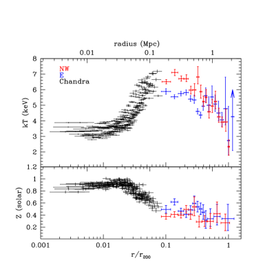
Figure 19: The observed, projected temperature ($kT$) and metallicity ($Z$) profiles in the Perseus Cluster, the nearest, massive galaxy cluster and brightest, extended extragalactic X-ray source. Suzaku results for the northwestern (NW) arm of the cluster are shown in red; and for the eastern (E) arm (approximately aligned with the major axis) in blue (Simionescu et al. 2011). Chandra measurements of the inner regions (Sanders & Fabian 2007) are shown in black.

Models of large scale structure formation show that gas is shock heated as it falls into clusters. Entropy is an important tracer of this virialization process. Numerical simulations predict that in the absence of non-gravitational processes such as radiative cooling and feedback, the entropy, $K$, should follow a power-law with radius, $K\ {\raise-3.22916pt\hbox{$\buildrel\propto\over{\sim}$}}\ r^{\beta}$, with $\beta\sim 1.1$–$1.2$ (e.g. Voit, Kay & Bryan 2005). With the exception of a cold front seen along the eastern arm at $r\sim 0.3r_{200}$, the entropy profile in Perseus roughly follows the expected trend out to $r\sim 0.6r_{200}$ (Figure 20). Beyond this radius, however, both arms flatten away from the predicted power-law shape. The pressure profile shows good agreement between the NW and E arms. Within $r\ {\raise-3.22916pt\hbox{$\buildrel<\over{\sim}$}}\ 0.5r_{200}$, the Suzaku pressure results show good agreement with the predictions from numerical simulations (Nagai, Kravtsov & Vikhlinin 2007), and previous measurements with XMM-Newton (Arnaud et al. 2010). At larger radii, however, the observed pressure profile is shallower than a simple extrapolation of the XMM-Newton results.

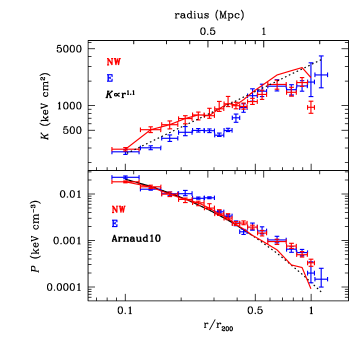
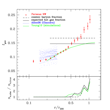
Figure 20: Left: Deprojected entropy ($K$) and pressure ($P$) profiles out to $r_{200}$ for the NW (red) and E (blue) arms of Perseus. In the upper panel, the black dotted line shows the expected, power-law entropy profile determined from simulations of non-radiative, hierarchical cluster formation: $K\propto r^{1.1}$ (e.g. Voit, Kay & Bryan 2005). In the lower panel, the black solid line shows a parameterized pressure model, motivated by simulations (Nagai, Kravtsov & Vikhlinin 2007), that was fitted to the inner regions ($r\ {\raise-3.22916pt\hbox{$\buildrel<\over{\sim}$}}\ 0.5r_{200}$) of clusters studied with XMM-Newton (Arnaud et al. 2010). The dotted curve is the extrapolation of this model to larger radii. The solid, red curves show the entropy and pressure profiles measured for the NW arm by Suzaku after corrections for gas clumping, which agree with the model predictions. Right: The integrated gas mass fraction profile for the NW arm of the Perseus Cluster. The dashed black line denotes the mean cosmic baryon fraction measured by WMAP7 (Komatsu et al. 2011). Accounting for 12% of the baryons being in stars (Lin & Mohr 2004; Gonzalez, Zaritsky & Zabludoff 2007; Giodini et al. 2009) gives the expected fraction of baryons in the hot gas phase, marked with the solid black line. Previous results at $r\leq r_{2500}$ from Chandra (Allen et al. 2008) are shown in blue. Predictions from numerical simulations (Young et al. 2011) incorporating a simplified AGN feedback model are shown in green. The bottom panel shows the overestimation of the electron density as a function of radius due to gas clumping. See Simionescu et al. (2011) for details.

Accurate estimates of the gas masses and total masses out to large radii are of particular importance for cosmological studies. The Suzaku observations of the Perseus Cluster provide the first such measurements for a massive cluster. The best-fit NFW mass model determined from a hydrostatic analysis of the (relatively relaxed) NW arm has parameters in good agreement with the predictions from cosmological simulations ($c=5.0\pm 0.5$, $M_{200}=6.7\pm 0.5\times 10^{14}\,M_{\odot}$) and provides a good description of the data (Simionescu et al. 2011). Of particular interest is the cumulative $f_{\mathrm{gas}}$ profile, shown in the right panel of Figure 20. Within $r_{2500}$ ($r\ {\raise-3.22916pt\hbox{$\buildrel<\over{\sim}$}}\ 0.3r_{200}$), the observed $f_{\mathrm{gas}}$ profile is consistent with previous Chandra and SZ measurements for other massive, relaxed clusters (Allen et al. 2004, 2008; LaRoque et al. 2006). From $0.2$–$0.45r_{200}$ (i.e. excluding the central cooling core) the $f_{\mathrm{gas}}$ profile is also consistent with the predictions from recent numerical simulations, incorporating a simple model of AGN feedback (Young et al. 2011). At $r\sim 0.6r_{200}$, the enclosed $f_{\mathrm{gas}}$ value approximately matches the mean cosmic baryon fraction, as measured from the CMB (Komatsu et al. 2011). Beyond $r\sim 2/3r_{200}$, however, where the entropy also flattens away from the expected power-law behavior, the $f_{\mathrm{gas}}$ apparently exceeds the mean cosmic value. The most plausible explanation for the apparent excess of baryons at large radii is gas clumping: in X-rays, the directly measurable quantity from the intensity of the emission is the average of the square of the electron density, rather than the average electron density itself. If the density is not uniform, i.e. the gas is clumpy, then the average electron density estimated from the X-ray intensity will overestimate the truth; this will lead to an overestimate of the gas mass and gas mass fraction, and will flatten the apparent entropy and pressure profiles.

The amount of gas clumping in Perseus, as inferred from comparison of the observed and expected $f_{\mathrm{gas}}$ profiles, is shown in the lower panel of the right of Figure 20. Using this clumping profile to correct the pressure and entropy measurements gives the solid red curves in the left panel. The clumping-corrected entropy profile shows good agreement with the expected power-law form out to $r_{200}$. Likewise, the clumping-corrected pressure profile matches the form predicted by simulations (Nagai, Kravtsov & Vikhlinin 2007).

Importantly, the Suzaku results provide no evidence for the puzzling deficit of baryons at $r\sim r_{500}$ inferred from some previous studies of massive clusters using lower quality X-ray data (at large radii) and stronger modeling priors (e.g. Vikhlinin et al. 2006; Gonzalez, Zaritsky & Zabludoff 2007; McCarthy, Bower & Balogh 2007; Ettori et al. 2009). The Perseus data suggest that beyond the innermost core but within $r\ {\raise-3.22916pt\hbox{$\buildrel<\over{\sim}$}}\ 0.5r_{200}$, X-ray measurements for massive, relaxed clusters can be used simply and robustly for cosmological work. At larger radii, the effects of gas clumping become increasingly important and must be accounted for.

In principle, the combination of X-ray and SZ observations can also be used measure gas clumping, offering an important cross-check of the Suzaku results. The origin of these density fluctuations is also an important, open question. Although numerical simulations predict that the gas in the outskirts of clusters should be clumpy (e.g. Mathiesen, Evrard & Mohr 1999), the degree of inhomogeneity predicted depends in detail on a range of uncertain physical processes, including cooling, conduction, viscosity, and the impact of magnetic fields.

Over the next few years, Suzaku and SZ studies of other bright, nearby clusters, complemented later by higher spectral resolution X-ray data from ASTRO-H, can be expected to stimulate significant progress. In particular, $f_{\mathrm{gas}}$ measurements out to large radii for a statistical sample of nearby clusters, and measurements of the dispersion in this and other properties from region-to-region and system-to-system, should provide a robust low-redshift anchor for cosmological work and powerful constraints on astrophysical models.

6.4 Evolution of Cluster Cores

Cluster cores – typically describing the central region of $r<50$–100$\mathrm{\,kpc}$ radius – often host a variety of astrophysical processes including efficient radiative cooling, AGN outbursts, modest star formation, and sloshing or other bulk motions (see, e.g., McNamara & Nulsen 2007 for a review). In the cores of even the most dynamically relaxed clusters, small-scale departures from hydrostatic equilibrium are often apparent (Fabian et al. 2003; Markevitch & Vikhlinin 2007; Allen et al. 2008).

The astrophysics of cluster cores is especially important for cosmological studies at X-ray wavelengths. In particular, clusters for which radiative cooling in the core is efficient form an easily distinguishable sub-population with significantly enhanced central gas density and luminosity, also commonly accompanied by a drop in ICM temperature (Fabian et al. 1994; Peterson & Fabian 2006). The sharp, central density peaks of these ‘cool core’ clusters enhance their detectability at X-ray wavelengths. However, without spatial resolution $\ {\raise-3.22916pt\hbox{$\buildrel<\over{\sim}$}}\ 10$ arcsec or additional follow-up data, cool-core clusters at high redshift lying close to the survey flux limit cannot be distinguished easily from non-cluster X-ray point sources. (This selection bias has affected some studies in the literature.) The prevalence and evolution of cool cores in the cluster population thus plays a significant role in determining the shape and evolution of the scatter in X-ray luminosity at fixed mass.

Confirmation of this fact can be found in the dramatic reduction in scatter obtained when emission from a central region of radius $0.15r_{500}$ is excised from luminosity measurements in forming the $L_{\mathrm{X}}$–$M$ scaling relation, from $\sim 40\%$ to $<10\%$ (Figure 21; see also Markevitch 1998; Allen & Fabian 1998; Zhang et al. 2007; Maughan 2007; Mantz et al. 2010a). (While the excision radius of $0.15r_{500}$ has become somewhat conventional, a similar reduction in scatter is evident when excising a fixed metric radius of similar size, e.g. 150$\mathrm{\,kpc}$.) Mantz (2009) found that roughly half of the intrinsic scatter can be attributed to radii $<0.05r_{500}$, the typical scale of cool, dense cluster cores, with most of the remainder due to variations in the gas density profile at $0.05<r/r_{500}<0.15$. The fraction of the total flux coming from $r<0.05r_{500}$ can be as large as 50%, and correlates strongly with other observable signatures of cool cores such as central cooling time and cuspiness of the surface brightness profile (Mantz 2009; see also Andersson et al. 2009). Interestingly, the fractions of cool-core systems identified using this criterion are comparable in X-ray flux-selected samples, at least within $z<0.5$ ($\sim 40\%$; see Figure 21; Peres et al. 1998; Bauer et al. 2005; Sanderson, Ponman & O’Sullivan 2006; Chen et al. 2007; Mantz 2009), although these fractions are biased relative to the full population due to selection effects. Cool cores are also common in X-ray selected samples at high redshift (Santos et al. 2008; $0.7<z<1.4$).

      

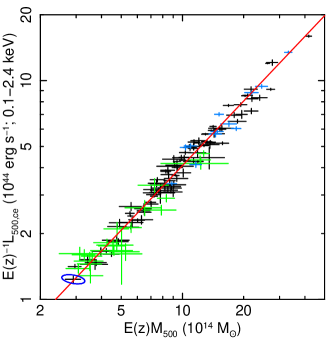
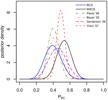
Figure 21: Left: Center-excised luminosity–mass relation, in which emission within $0.15r_{500}$ of cluster centers is excluded from the luminosity measurements. Error bars in the plot show statistical uncertainties only. The intrinsic scatter in this relation is $<10\%$, significantly reduced from $\sim 40\%$ for the full luminosity–mass relation. Gray points are at redshifts $z<0.5$, blue points are at $0.5<z<0.7$, and green points are at $0.35<z<0.9$. The blue ellipse shows the typical correlation of measurement errors, which is accounted for in the fit. The negative sense of the measurement correlation results from details of the center excision: larger mass implies larger $r_{500}$ and thus a larger excised region. Since more flux is excised than is gained at large radius when $r_{500}$ increases, there is a net reduction of luminosity with larger mass. From Mantz et al. (2010a). Right: Posterior probability distributions for the fraction of cool-core clusters based on the number identified in various X-ray selected samples at $z<0.5$. Due to Malmquist bias, these must overestimate the fraction in the full cluster population. From Mantz (2009, see also references therein).

Although the number of massive clusters found in RASS is too small to detect evolution or departures from log-normality in the luminosity–mass scatter, future, deeper X-ray surveys such as eROSITA will provide the larger samples necessary for these investigations. Conversely, a better understanding of cluster cores will be required to fully exploit these surveys for cosmology. Such studies will need to employ the full statistical apparatus described in Section 4.1.1 to obtain unbiased results.

Due to the weaker dependence of the SZ signal on the central gas density (Section 3.1), SZ surveys are expected to be less sensitive to the presence of cool cores than X-ray surveys. This is consistent with the relatively low fraction of cool core systems observed among the newly discovered clusters in the Planck Early Release cluster catalog (Planck Collaboration 2011a, d). We note, however, that current SZ surveys are not necessarily immune to biases associated with cool cores; depending on the selection techniques employed, infrared emission associated with star formation in the central regions of cool core clusters may actually diminish the measured SZ signal.

6.5 Improved Simulations

Unleashing the full statistical power of upcoming surveys will require careful control of theoretical uncertainties. For cluster abundance and evolution tests, uncertainties in scaling relation parameters are currently more important than uncertainties in the halo mass and bias functions (Cunha & Evrard 2010). With aggressive mass calibration efforts to reduce the former, the mass function and bias errors will need to be limited to the percent level in order to avoid significant degradation in cosmological parameter constraints (Wu, Zentner & Wechsler 2010). Simulation campaigns will be needed to address this challenge.

Over the next decade, increased computing power will enable models with new capabilities (e.g. multi-scale simulation in place of sub-grid models) and will vastly expand the size of current simulation suites. By densely sampling a large control space of cosmological and astrophysical parameters, simulation ensembles can support survey analysis via functional interpolation, a method termed emulation (Habib et al. 2007). An initial application of this technique uses 38 $10^{9}$-particle N-body simulations to predict the non-linear matter power spectrum to $1\%$ accuracy (for $k\ {\raise-3.22916pt\hbox{$\buildrel<\over{\sim}$}}\ 1\ h/\mathrm{\,Mpc}$) in a 5-dimensional space of cosmological parameters (Lawrence et al. 2010).

Precise N-body calibrations must be treated with some caution, as the baryons representing $17\%$ of the total mass undergo different small-scale dynamics than CDM. Back-reaction effects of cooling and star formation could be important (Rudd, Zentner & Kravtsov 2008; Stanek, Rudd & Evrard 2009) and should be systematically investigated. As discussed in Sections 4.5 and 5, studies of LSS in non-standard cosmologies, including those for which dark energy may cluster or in which weak-field gravity is non-Newtonian, should also be pursued.

Full solution of the galaxy formation problem from first principles remains challenging. Direct simulation methods will continue to improve, though not likely to the point where multi-fluid simulations will offer definitive predictions for next-generation survey analysis. Semi-analytic methods are increasingly informative; for example, the frantic early merging that forms the central galaxies in clusters is becoming understood (De Lucia et al. 2006; Weinmann et al. 2010). But many elements required to predict the spectrophotometric properties of galaxies remain poorly understood, including stellar population synthesis and dust evolution (Conroy, White & Gunn 2010). Empirically tuned statistical approaches, essentially assigning galaxy properties to halos or sub-halos in a manner informed by observed clustering as a function of luminosity and/or color, will continue to provide a valuable complement to physical methods.

Upcoming surveys will require sophisticated, automated reduction and analysis pipelines for their large data streams, along with quality assurance to validate accuracy. Simulations of sky expectations, often referred to as ‘mock’ or ‘synthetic’ surveys, will be required to provide realistic testbeds in which the answers are known. Mock surveys provide key quality assurance support by: (i) incorporating line-of-sight projection effects on measured properties; (ii) including distortions and noise from telescope/camera optics and other sources; and (iii) validating image processing and data management pipelines. Since the effort involved in producing such data is non-trivial, mechanisms to publish and enable their broader use within the community need to be pursued.

7 MODELING CONSIDERATIONS

With such significant improvements in data quality expected and such profound questions to be addressed, modeling considerations will become increasingly important. The key issues will be modeling and mitigating all important sources of bias and systematic error in the analyses, and using the information efficiently.

For tests based on the mass function and clustering of clusters and their associated mass–observable scaling relations, the impact of survey biases must be accounted for (Section 2.5.1). Typically this requires simultaneous modeling of the cluster population and scaling relations in a single likelihood function. Such an approach also facilitates understanding the covariance between model parameters, and provides a structure within which to examine the impact of residual systematic uncertainties which often correlate with model parameters. To a large degree, the statistical frameworks required for such analyses have been developed (Section 4.1.1) and their application to existing data are discussed in this review.

The application of judicious, blind (see below) cuts can improve the balance of statistical versus systematic uncertainties. For example, with the $f_{\mathrm{gas}}$ test (Section 4.2), cosmological constraints are best derived from the most massive, dynamically relaxed clusters, which can be identified easily from short, snapshot Chandra or XMM-Newton X-ray observations. These clusters are also ideal targets for the XSZ test (Section 4.3). For the mass function and clustering tests, one must determine the optimal mass/flux/redshift range over which to compare the data and models, given the characteristics of the survey and follow-up data and one’s understanding of mass–observable scaling relations.

Strong priors should be used with caution and their implications understood. In cluster cosmology, common assumptions include log-normal scatter in the mass–observable scaling relations, and negligible evolution of this scatter with redshift. When measuring masses from X-ray or optical dynamical data, the use of parameterized temperature, velocity and gas density models is also common. Where such strong assumptions are not necessary, they should be avoided. Where priors do become necessary, for example in parameterizing the impacts of known astrophysical effects, the validity of these assumptions should be checked empirically, where possible.

The covariance between different measured quantities is an important consideration that is often wrongly neglected. The simplest example of this is simply the statistical correlation of quantities measured from the same observation (e.g. due to Poisson noise). A more subtle case follows from the definition of cluster radius for scaling relations in terms of the mean density enclosed: because the measured mass and radius covary, other quantities measured within that radius necessarily covary with mass, even if measured from independent observations. Fortunately, within the framework of Bayesian analysis, it is straightforward to account for such measurement correlations. For example, given a set of scaling relation parameters to be tested, the data likelihood can be integrated over all possible true values of, e.g., the mass and temperature, with one of the terms in the integrand being the probability of the true mass and temperature values producing the observed values (the sampling distribution; see Section 4.1.1). The form of this probability density can be as general as is required – a multidimensional gaussian or log-gaussian in the simplest case – and in particular may have non-zero correlation. Kelly (2007, see also ) discusses this general approach in the astrophysical context, and provides useful tools for Bayesian linear regression.

In other situations, unnecessary covariance can be introduced by the model applied to the data. An example is the historically common practice of fitting parametric temperature and gas density profiles to X-ray data, and inferring overdensity radii and hydrostatic masses from these model profiles. Here, the procedure introduces an artificial covariance between mass and temperature (i.e. a prior on the scaling relation) which could be avoided simply by modeling the temperature and gravitating mass profiles independently.

Where binning will result in a loss of relevant information, it should be avoided. For example, the binning of X-ray surface brightness data to determine an integrated X-ray luminosity results in a significant loss of information; the center-excised luminosity provides a tighter mass proxy (Section 6.4).

Hypothesis testing will remain a critical element of future analyses. Wherever a model is fitted to data, one should check that it provides an adequate description (i.e. that the goodness of fit is acceptable); if it doesn’t, then the model can be ruled out. This is particularly important in the context of cosmological surveys and scaling relations that are subject to selection bias, since no straightforward, visual check of the goodness of fit is typically possible. Where the simplest models fail to describe the data, one must evaluate carefully the additional degrees of freedom needed to alleviate the tension, in particular considering both astrophysical and cosmological possibilities; simulations will play a critical role in motivating and validating alternatives to the simplest scaling models. A related situation arises in the combination of constraints from independent experiments: before combining, one should ensure that the model in question provides an adequate description of the data sets individually, and that the parameter values are mutually consistent, i.e. that their multi-dimensional confidence contours overlap. Here it can be helpful to include the impact of all known systematics in the contours; where contours do not overlap, the model is incomplete and/or unidentified systematic errors are present. Historically, the combination of mutually inconsistent data sets has sometimes led to unphysically tight formal constraints.

Training sets can be useful to tune analyses. However, the biases introduced by this training must be understood and accounted for. The inclusion of sufficient redundancy into experiments (i.e. having more than one independent way to make a measurement) can also enhance significantly the robustness of conclusions. In cosmological studies, for example, we require more than a single way to measure both the growth and expansion histories, e.g. clusters and lensing, and SNIa and BAO, respectively.

A final modeling consideration is the impact of experimenter’s bias: the subjective, subconscious bias towards a result expected by an experimenter. This is important where we are seeking to measure a quantity for which prior expectations exist, e.g. $w$ or the growth index, $\gamma$. Evidence for experimenter’s bias can be found readily in the literature, e.g. in historical measurements of the speed of light or the neutron lifetime (see Klein & Roodman 2005 for a review). The best approach to overcoming experimenter’s bias is blind analysis.

A range of blind analysis techniques are commonly employed in the particle and nuclear physics communities. These are used to mask the ability of scientists to determine quantities of interest until all methods are finalized, the systematic errors that can be identified have been, and the final measurement is ready to be made. A technique with good applicability to cosmological studies is hiding the answer, wherein a fixed (unknown to the experimenter) offset is added to the parameter(s) of interest, and only revealed once the final measurements are made. Before un-blinding, it is advisable to think through how to proceed afterward, and what additional checks to employ. Double-blind analyses, where two independent teams repeat the same process (often used in biomedical research) target additional sources of error. Such techniques can be used powerfully, where resources allow.

8 CONCLUSIONS

Our article has summarized the status of cluster cosmology and the methods used to extract cosmological information from galaxy cluster observations. These methods have been applied successfully to samples of tens to thousands of massive clusters. Much of this work has been pioneered at X-ray and optical wavelengths, but SZ surveys and gravitational lensing studies are also now poised to play central roles.

The availability of powerful, new cluster surveys will help to address profound mysteries such as the origin of cosmic acceleration, inflation and the nature of gravity. This work will require a multiwavelength approach, combining the strengths of the available techniques for finding clusters, calibrating their masses and obtaining low-scatter mass proxies. The analysis of these data will require dedicated efforts by large teams of researchers. The demands for follow-up observations will be high, and will require the support of time allocation committees.

Building on the progress made, we can expect clusters to remain at the forefront of cosmological work through the next decade. By combining cluster measurements with other, powerful probes such as SNIa, CMB, BAO and cosmic shear, we can be optimistic of having the precision, complementarity and redundancy required to allow robust conclusions to be drawn.

References

- Abel, Bryan & Norman (2002) Abel T, Bryan GL, Norman ML. 2002. Science 295:93–98
- Abell (1958) Abell GO. 1958. ApJS 3:211–288
- Abell, Corwin & Olowin (1989) Abell GO, Corwin Jr. HG, Olowin RP. 1989. ApJS 70:1–138
- Ackermann et al. (2010) Ackermann M, Ajello M, Allafort A, Baldini L, Ballet J, et al. 2010. J. Cosmology Astropart. Phys. 5:25
- Acquaviva et al. (2003) Acquaviva V, Bartolo N, Matarrese S, Riotto A. 2003. Nuclear Physics B 667:119–148
- Allen, Ettori & Fabian (2001) Allen SW, Ettori S, Fabian AC. 2001. MNRAS 324:877–890
- Allen & Fabian (1998) Allen SW, Fabian AC. 1998. MNRAS 297:L57–L62
- Allen et al. (2008) Allen SW, Rapetti DA, Schmidt RW, Ebeling H, Morris RG, Fabian AC. 2008. MNRAS 383:879–896
- Allen et al. (2004) Allen SW, Schmidt RW, Ebeling H, Fabian AC, van Speybroeck L. 2004. MNRAS 353:457–467
- Allen et al. (2003) Allen SW, Schmidt RW, Fabian AC, Ebeling H. 2003. MNRAS 342:287–298
- Amin, Wagoner & Blandford (2008) Amin MA, Wagoner RV, Blandford RD. 2008. MNRAS 390:131–142
- Andersson et al. (2010) Andersson K, Benson BA, Ade PAR, Aird KA, Armstrong B, et al. 2010. arXiv:1006.3068
- Andersson et al. (2009) Andersson K, Peterson JR, Madejski G, Goobar A. 2009. ApJ 696:1029–1050